
Geometric Outlines of the Gravitational Lensing and Its Astronomic Applications

School of Mathmatics, Southeast University, Nanjing 211189, China
*
Author to whom correspondence should be addressed.
†
These authors contributed equally to this work.
Universe 2023, 9(3), 153; https://doi.org/10.3390/universe9030153
Submission received: 13 February 2023
/
Revised: 13 March 2023
/
Accepted: 13 March 2023
/
Published: 17 March 2023
(This article belongs to the Collection Modified Theories of Gravity and Cosmological Applications)
Abstract
:Gravitational lensing is a topic of great application value in the field of astronomy. The properties and research methods of gravitational lensing are closely related to the geometric and relativistic characteristics of the background universe. This review focuses on the theoretical research and application of strong lenses and weak lenses. We first introduce the basic principles of gravitational lensing, focusing on the geometric basis of geometric lensing, the representation of deflection angles, and the curvature relationship in different geometric spaces. In addition, we summarize the wide range of applications of gravitational lensing, including the application of strong gravitational lensing in Schwarzschild black holes, time delay, the cosmic shearing based on weak lensing, the applications in signal extraction, dark matter, and dark energy. In astronomy, through the use of advanced astronomical instruments and computers, analyzing gravitational lensing effects to understand the structure of galaxies in the universe is an important topic at present. It is foreseeable that gravitational lensing will continue to play an important role in the study of cosmology and will enrich our understanding of the universe.
Keywords:
gravitational lensing; deflection angle; Einstein ring; Schwarzschild black hole; dark matter and dark energy; time delay; cosmic shearMSC:
85-061. Introduction
Light rays are deflected in a gravitational field. The light of the background galaxy is focused by the gravitational field of the foreground galaxy. Such a light deflecting phenomenon, which is similar to that observed in an optical lens, is called gravitational lensing. Einstein’s general theory of relativity first predicted and explained the phenomenon of gravitational lensing [1]. The first lens system, QSO 0957+561A, B, was discovered in 1979 [2]. Since then, increasing attention has been paid to the research of gravitational lensing. Currently, gravitational lensing can be divided into three categories (i.e., strong gravitational lensing, weak gravitational lensing, and microlensing) based on the geometric configuration among the background galaxy, the foreground galaxy, and the observer, as well as the mass–energy distribution of the foreground galaxy. Strong gravitational lensing can produce multiple and severely distorted images [3]. However, it can greatly brighten the lights from distant galaxies, which is quite spectacular. Thus, strong gravitational lensing is often used to study distant galaxies [4]. Unlike strong gravitational lensing, weak gravitational lensing is more common and produces slightly distorted images [5]. It has more applications, for example, as the information from weak lensing is necessary to reveal the whole mass distribution of the cluster.
Gravitational lensing has valuable applications, especially in the detection of dark matter and dark energy, which do not emit electromagnetic radiation but constitute contents of the universe. However, dark matter is a major component of matters with gravitational effects. In addition, considering the relationship between gravitational lensing, dark energy, and the large-scale structure evolution of the universe, gravitational lensing can also be one of the detection tools of dark energy. Furthermore, we can use gravitational lensing to study the cosmological parameter, the Hubble constant, and the age and density of the universe [6]. Recently, Jee I. et al. proposed a method to determine the Hubble constant by using the angular diameter distance to strong gravitational lenses as a suitable calibrator [7].
Moreover, gravitational lensing was also adopted to investigate the black holes and wormholes. Recently, Bohn et al. analyzed a binary black hole merger [8]. Lu and Xie studied an Extended Uncertainty Principle black hole [9]. Sharif et al. numerically evaluated the deflection angles in the strong field limit to find the locations of wormholes [10]. Ono T. et al. studied the deflection angle of light for an observer and source at a finite distance from a rotating Teo wormhole, and the correction of the deflection angle due to the limited distance from the rotating wormhole was obtained [11]. Takahashi et al. discussed the negative-mass compact objects and the number density of Ellis wormholes [12]. Ovgun applied the Gauss–Bonnet theorem to Damour–Solodukhin wormhole spacetimes to probe weak gravitational lensing [13]. Recently, researchers focus on the black hole shadow, which is the dark region in the center of a black hole image. It appears because the light rays are close enough to be captured by the black hole itself, thereby leaving a black shadow in the observer’s visual field. Perlick et al. proposed the derivation of the angular magnitude of shadows in static sphere symmetric spacetime. They calculated the black hole shadows in the expanding universe and also considered the effect of plasma on black hole shadows [14]. Akiyama et al. assembled the Event Horizon Telescope. The images they observed were consistent with the prediction of general relativity concerning the shadow of the Kerr black hole [15]. In addition, the first observation of Sagittarius A* (Sgr A*) using the Event Horizon Telescope (EHT) can be found in [16]. The gravitational lensing effect is also of great value for gravitational wave detection. For example, Cao et al. analyzed the influence of lenses on gravitational wave signal parameters [17]. Oguri used gravitational lensing magnification to analyze the distribution of gravitational waves generated by binary star mergers [18]. Today, various emerging technologies have also been used to explore gravitational lensing, such as convolutional neural networks [19] and 3D printing technology [20]. With the further development of science and technology, it is foreseeable that the study and application of gravitational lensing will be improved, which would help us understand the vastness of universe on a deeper level.
In this manuscript, we first briefly introduce the fundamental principle of the gravitational lensing in Section 2. Then, we discuss the progress of the strong lensing of a Schwarzschild black hole and the time delay in Section 3. Subsequently, cosmic shear, signal extraction, dark matter, and dark energy detection based on weak lensing are introduced in Section 4. For a better understanding of gravitational lensing, we recommend the following references [21,22,23,24].
2. Fundamental Principle
2.1. Deflection Angle
When a photon passes by a massive object, such as a galaxy or a galaxy cluster, the deflection of its trajectory is described by the deflection angle . Assuming the effective refractive index , one can obtain from the Fermat’s principle that
where is the scalar Newtonian potential that obeys the Poisson’s equation. Here, we use to denote the angle with a direction since the right-hand side of (1) is an integral of a vector. However, we will denote the angle without the arrow in this manuscript since we are more concerned about the magnitude of the angle than its direction.
For a point lens, in Newtonian mechanics, the deflection angle is deduced from (1) to be
where M is the mass of lens and b is the closest distance of the photon to the lens, while, in General Relativity, the deflection angle of a point lens with gravitational potential is deduced to be
which is twice of that in Newtonian mechanics. However, the deflection angle of light is small and generally on the order of arc–sec.
Takizawa et al. [25] defined the deflection angle of light () in an integral form to eliminate the asymptotically flatness of space–time. Namely,
where is a trilateral specified by the points R, , and , and is a trilateral specified by the points S, , and . The right-hand side of (2) contains the radial coordinate , where means the closest approach of light. Ishihara et al. [26] defined the deflection angle of light () under the assumption of asymptotic flatness as
in which and are the angles between the radial direction and the light ray at the source position and at the receiver position, respectively. is a coordinate angle between the receiver and source. Without the assumption of asymptotic flatness, Takizawa et al. [25] proved the consistency of the above two definitions on a static and spherically symmetric spacetime, i.e.,
In [27], Takizawa et al. also defined a deflection angle as
in which denotes the angular direction of the lensed image with respect to the lens direction. It follows from (3) and (5) that
where we use . One can deduce from (4) and (6) the equivalence of the above three definitions.
The gravitational lensing deflection angle can reflect the overall geometry of the foreground universe. In 2008, Gibbon and Werner first proposed a mathematical method to measure the asymptotic deflection angle of the gravitational lenses adopting the Gauss–Bonnet method [28]. In 2012, Werner discovered that for a stationary observer in the Kerr spacetime, a spatial light ray is a geodesic in a certain Randers metric space [29]. Given that a light ray is in a geodesically complete surface whose Gaussian curvature in the optical geometry is K. It can be shown that its asymptotic deflection angle is
where the integral is used over the infinite region of the surface bounded by the light ray excluding the lens. Based on the same approach, in 2020, Halla and Perlick used the Gauss–Bonnet theorem to provide a mathematical representation of the deflection angle of gravitational lenses in the NUT metric space [30].
As a generalization of traditional geometric backgrounds, Finsler background spacetime, especially Randers spacetime, has a wide range of physical applications. There is also a corresponding deflection angle definition on it. We refer to [31] for more details of the underlying geometry of the SFR gravitational model, as well as the field equations for the SFR metric. Kapsabelis et al. [31] derived the deflection angle in SFR spacetime as
Expanding (8) in powers of , the deflection angle can be written as follows:
where J is the angular momentum, and is a constant obtained when solving field equations.
Compared to the deflection angle in General relativity, includes a small additional Randers contribution term s, which yields a slight deviation from . Considering by , it follows that
The difference between the deflection angle in SFR spacetime and may be due to Lorentz violations [32], or the small amount of energy that is added to the gravitational potential of SFR.
Recently, the first author of this work introduced, for the first time, the asymptotically Minkowskian flat properties on the general Finsler metric manifold. Moreover, an integral representation of the integral symmetric normal deflection angle of the gravitational lens on an asymptotic symmetric Minkowskian flat Finsler manifold in a large range was provided [33]. Concretely,
where is a region bounded by the deflection light, L and are the lengths of the indicatrixes at the infinity and at x, respectively, is the T-curvature, K is the Gauss curvature, and J is the Landsberg curvature. Formula (11) is a generalization of (7) and can be adopted to illustrate a new geometric explanation of dark matter and dark energy, as well as their effects.
2.2. Lens Equation
In general, the scale of the lens is much smaller than both the distance from the light source to the lens and the distance from the lens to the observer . Therefore, the lens is often reduced to fall on a flat surface. For lenses with a mass distribution of , we use to represent the position vector on the plane of the lens. Its surface mass density is provided by . Then, the deflection angle at is
in which we call the Schwarzschild radius.
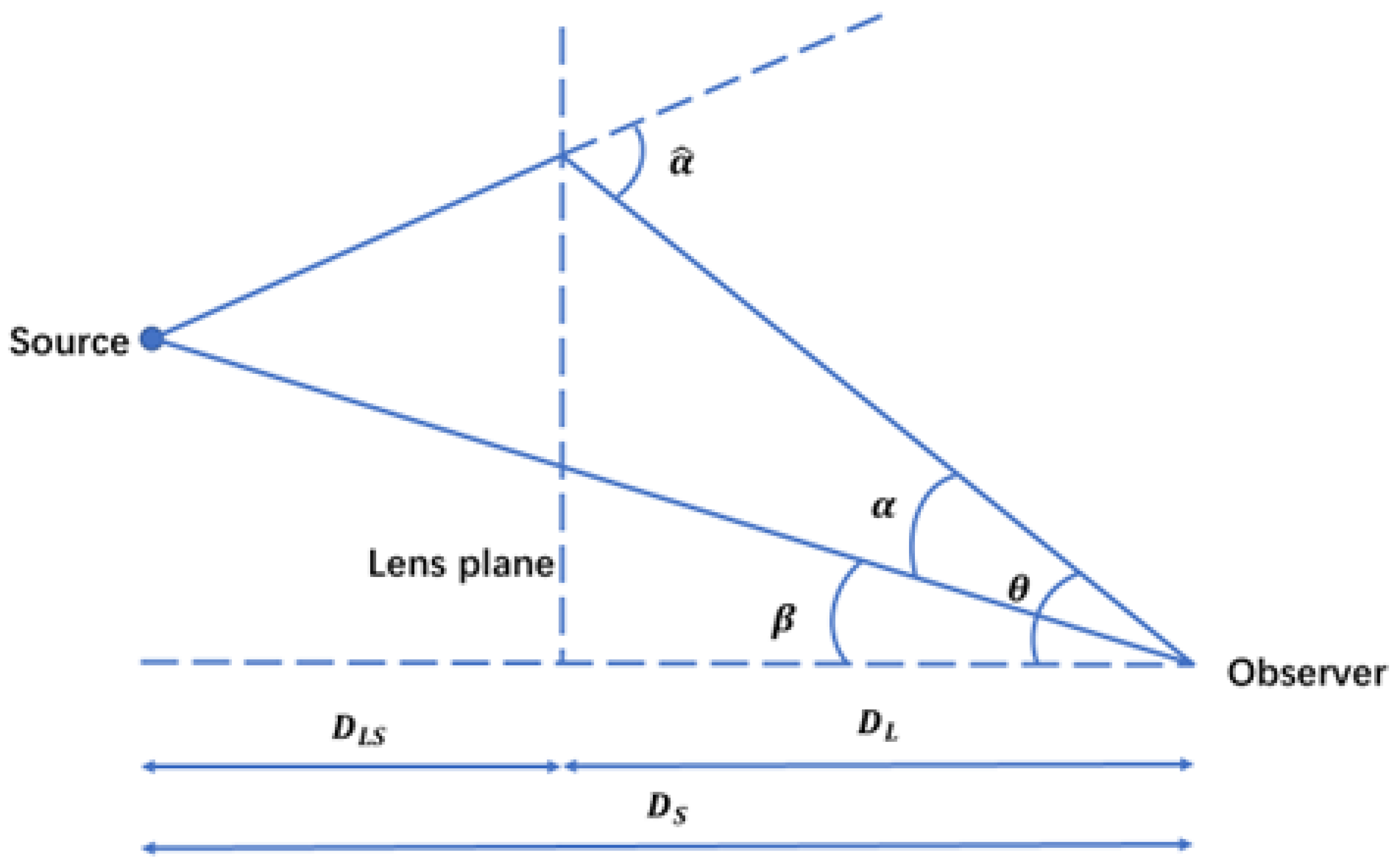
The line-of-sight dominates the plane of the light source, the plane of the lens, and the optical axis of the observer. Without a lens, the observer will see the light from the light source at an angle of to the optical axis. Under the gravitation of massive objects, the observer will see the angle . Thus, using geometric relations, under the setting , we can write it as
where (13) is known as the lens equation and has further expression and applications [34,35]. A schematic geometry of the lens equation can be seen in Figure 1.
Equations (12)–(14) are classic lens equations in gravitational lensing. Nowadays, the study of lens equations has been further advanced and different forms have been proposed. We introduce more definitions of the deflection angle, as well as a class of exact gravitational lens equations at finite distances.
Takizawa et al. deduced the exact gravitational lens equation for (in Equation (5)) as
They also considered a static and spherically symmetric solution in Weyl conformal gravity, and provided iterative solutions for the finite-distance lens equation up to the third order.
Furthermore, Takizawa et al. [36] showed that the hyperbolic (spherical) trigonometry can be used in the exact lens equation for a de-Sitter (anti-dS) background and discussed possible effects by the curvature of the dS/AdS background. Moreover, they provided a unified form of Lens equations in Euclidean, hyperbolic, and spherical geometry by
where the parameters with corner markers are normalized defined quantities, and K denotes 1, 0, and for spherical, flat, and hyperbolic geometry, respectively. Based on the curvatures of the dS/AdS background, they presented the deflection angle in dS/AdS background by
in which for the mass m. Although dS and AdS are geometrically different, their deflection angles are formally the same.
In small angle approximations, the difference in the form among the dS/AdS lens equations and the exact lens equation in the Minkowski background begins at the third order. The angular separation of the lensed images is decreased by the third-order deviation in the dS lens equation, while it is increased in AdS.
An Einstein ring occurs when the source, lens, and observer are aligned well. That is, using in (13), we can obtain the angular radius of the ring, namely, the Einstein radius, as
The property of the Einstein ring is special when there is a point source. In this case, Equations (12), (18), and (19) provide that
which can be solved by
Therefore, we can obtain that the angular radius of Einstein’s ring is by setting in (21).
The magnification of an Einstein ring is
where is the solid angle covered by the lensed image, and denotes the angle in the absence of the lens.
For Einstein rings, noticing the geometric relationship between the source, the lens, and the observer (i.e., the axisymmetric property), one can simplify (22) as
Hence, we can deduce the magnification of an Einstein ring from (23) as
where represents the true angular radius of the source.
In the case of the imperfect alignment of sources, lenses and observers, i.e., , the angular separation between the two images is deduced from (23) and (21) as
Hence, the magnification is
Moreover, the total magnification is
The figure of an Einstein ring as a smiley in the following link, taken by the NASA/ESA Hubble Space Telescope: https://images.nasa.gov/details-GSFC_20171208_Archive_e000791 (accessed on 14 January 2023).
2.3. Convergence and Shear
Lens Equation (13) could be considered as a mapping from the source plane to the lens plane. It can especially be linearized to obtain local information of the mapping. The Jacobian matrix of (13) has component , which could be decomposed into two parts as
where and are the convergence and shear parameters, respectively, defined by
where is the lensing potential, whose expression is
Furthermore, , so that (13) could be rewritten as
in (28) is named as the critical surface mass density, and is defined by . is a parameter of homothetic transformation, indicating that the light source is isotropically amplified or reduced. Meanwhile, adds anisotropic effects to the imaging. The distortion of the image can be described by the inverse matrix of the above Jacobian, which is denoted by .
By the eigenvalues of the Jacabian matrix A, one can determine the radial elongation factor to be , and the tangential factor to be . It follows for that
These imply that the convergence and the shear are
For , the lensing shear can be similarly obtained as
For cases where the position of the lens is unknown, the origin of the two-dimensional coordinates can be selected as the center of the lens object. For a pair of radially elongated images , they are aligned with each other, while, for a pair of tangentially elongated images, they are parallel to each other. Thus, radial and tangential elongations can be distinguished by measuring such image alignment in observations.
In the weak field and thin lens approximation, the image is tangentially elongated due to the gravitational action of the lens model on the light, while the gravitational repulsion of light by the other models always radially distorts. This feature of the shape of the lens image can be used to search for (or confine) local exotic matter or energy. For more details and developments, we recommend [37].
In fact, cosmic shear is based on measurements of the shape of galaxies, so what is really observed is not the shear but the reduced shear , which has the same spin-two transformation properties as the shear.
In addition, the magnification of the image, denoted by , can be expressed by the inverse of the determinant of the Jacobian matrix, i.e.,
Furthermore, according to (37), the image is magnified, i.e., , so it looks brighter than the source.
Curves with infinity magnification, namely, , in the image plane are called critical curves. The corresponding curves on the source plane are called caustic curves. If a source is located near a caustic curve, it will be highly amplified and distorted. For example, it may create a huge arc in a star cluster. However, the magnification is not infinite, and a source will only produce one image, provided that the magnification of a gravitational lens is limited anywhere.
3. Strong Gravitational Lensing
In addition to the Einstein ring mentioned above, which has a tremendous visual aesthetic, we can also observe other important strong lensing phenomena. The observation and application of these phenomena have helped us further promote the development of cosmology and the advancement of modern technology.
For strong gravitational lensing, there are many observable values, such as the relative position of the image, the relative flux of the image, and the time delay of the change in luminosity between the lens images. These observables depend not only on the mass distribution of the source but also on cosmological parameters [23]. A mass model of the light source can be built to solve the lens equation with the help of light trace quality (LTM) or non-LTM methods. Today, based on these two methods, there is a lot of software code for strong lens models that can be applied.
Strong lenses can also be used to obtain the magnification of images [38]. Although we do not know the brightness of the light source, the ratio of the luminosity between images is observable. For the observed images A and B, we have
where M is the magnification matrix. Formula (38) can be considered as a linear transformation between two lens image spaces. On the other hand, the flux ratio is also an important constraint of the mass model of the lens.
In this section, to demonstrate the effective application of the strong lensing, we introduce the ongoing field of it, including Schwarzschild black hole and time delay.
3.1. Schwarzschild Black Hole
The deflection angle has already been briefly introduced in the last section. In this section we describe the deflection angle in the Schwarzschild’s black hole and the considerable measurements in it. The strong field limit coefficients and the deflection angle of the black holes can be obtained by performing the strong field limit method, which is a basic approach of this topic. For instance, Chagoya et al. [39] adopted a hybrid analytic–numerical approximation to determine the deflection angle in Schwarzschild spacetimes. Similar research on deflection angles and related applications can be found in [40,41,42]. The general Schwarzschild metric is defined by
where and are functions of r. The corresponding photosphere equation is
The maximum root of (40), denoted by , is called the radius of the photosphere.
For photons from the infinity, when approaching a black hole, there exist deviations from their original orbits. Let u nr the collision parameter, and be the minimum radial distance of a photon from the black hole during the traveling. The relationship between u and obeys the conservation of the angular momentum as
We may choose in (39) for the spherical symmetry of space–time. Therefore, from the radial equation of the photon
the expression of the deflection angle becomes [43]
in which and are the values of and at , respectively. The deflection angle depends on . More precisely, increases as reduces. It requires that for the photons to be fully absorbed. According to the bijective correspondence of and , the deflection angle can be represented by as
which is the deflection angle equation under strong field approximation. The two strong field limit coefficients and in (43) could be deduced as
where the quantities marked with the subscript m indicate the values of them at . The specific measurement parameters may be clarified by observing the strong field effect. Based on it, the structure of the lens should be detected.
3.2. Time Delay
Light travels along geodesics in curved space. The effect of gravity will increase the distance and cause a difference in time compared to the situation without gravity, which is called the time delay. In this case, we will only describe the propagation of light from sources at a great distance from the lens.
When light travels far from the lens, its path could be regarded as the geodesic in the Friedmann–Robertson–Walker gauge, which is an exact solution of Einstein’s field equations
where is the cosmic scale factor, which determines the geometric scale of the space. Denoting the closest point on the light path to the lens by P, the intrinsic length of the light path from the source to P and from P to the observer is
in which and are the moments when the photon leaves the source and reaches the observer, respectively. However, the time it requires for a photon to reach the observer without the lens is
in which is the intrinsic distance along the geodesic from the source to the observer, and is the moment when the photon arrives at the observer. Therefore, comparing (45) and (46), the time delay is
Another expression of (47) is the following, with the assistance of the geodesic equation, that is
where and are the normal radial coordinates of the source S and the point P, respectively, and is the angle between the observer-to-source connection and the observer-to-P connection.
Accounting for the cosmic redshift effect, that is, and using , (48) could be modified to be
Time delay has been employed to determine the Hubble constant, but it is imprecise due to insufficient astronomical observations.
A smoothness condition is imposed on the gravitationally deformed paths followed by the photons from the source to the observer. Maggiore, N., et al. [44] considered an alternative formula for time delay, which was generalized to the arbitrary angles of the standard one. It can be applied to investigate the discrepancy between the various estimations of the Hubble constant.
Inspired by its various effective applications, the research of time delay has been developed rapidly. It provides a powerful cosmological detector through the time delay distance.
However, it is not easy to achieve the ideal effect, because the images have the measurement gap, noise, and no prior function model, which causes the robust time delay estimation to be challenging. In fact, Hojjati et al. [45] used Gaussian process techniques and was successfully demonstrated in an accurate blind reconstruction of time delays and a reduction in uncertainties for real data. The results will be more accurate in the future when more information is accumulated.
4. Weak Gravitational Lensing
Strong gravitational lensing causes a large signal and produces phenomena that look extremely spectacular, such as Einstein rings and Einstein crosses. However, such phenomena rarely occur.
Conversely, there are a large number of weak gravitational lensing signals in the universe because the universe is filled with various structures, such as dark matter halos, fibers, etc. Especially in the past two decades, research on weak lenses has flourished. Moreover, weak gravitational lensing plays an important role in the field of astronomical detection [46,47,48]. Theoretically, if we can accurately measure information such as the deformation and redshift of galaxies in the universe, it is possible to reconstruct the distribution of matter in the whole universe, because the lens signal can reflect the information of matter in the path. The combination of lens signals with different redshifts provides ways to accurately determine the fundamental parameters in cosmology, such as , , .
As related to the Schwarzchild black hole, a static and spherically symmetric modified spacetime metric depends on the inverse distance to the power of positive n ( for Schwarzschild metric, and for an Ellis wormhole) in the weak-field approximation. Izumi, K., et al. obtained the following deflection angle in such space–time [37].
where is the book-keeping parameter. Under the thin lens approximation, the modified lens equation becomes
For the case of , the matter (and energy) need to be exotic if ; (51) could be rewritten as the following in the vectorial form.
where we normalize and for the angular position of the image , , and denote the corresponding vectors.
4.1. Cosmic Shear and E/B Modes
At present, cosmic shear is extremely important in the physical study of weak lensing, since its signal can reflect the distribution of matter and limit the cosmological parameters [49,50,51].
Nicola et al. [52] puts predictive constraints on the cosmological and mass calibration parameters for a combination of LSST cosmic shear and Simons Observatory tSZ (thermal Sunyaev-Zel’dovich) cluster counts. They found competitive constraints on cluster cosmology. Mancini et al. [53] studied 3D cosmic shear and Minkowski functionals, and demonstrated parameter inference from Minkowski functionals in a cosmic shear survey. Their work is the first step toward the use of Minkowski functionals as a probe of cosmology beyond the regular method of two-point statistics.
Convergence and shear are briefly described in Section 2.3. In fact, utilizing the Fourier transform, they can be connected as
where the quantities marked with indicate the corresponding values in the Fourier transformation.
Cosmic shear could be adopted to measure the coherent distortion of background galaxies, determine the matter–power spectrum, and illustrate the properties of dark matter. Technically, we represent the distance prefactor as
so that (31) is equal to
where is the co-moving angular–diameter distance.
From (28) and (56), considering the extended lens, we can deduce the convergence to be
where is the mass density.
Equation (57) means that is the geometrically weighted line-of-sight integral of . Noticing that and its cosmological mean value are provided by
where is the dimensionless density contrast, is the Hubble constant, and is the dimensionless matter–density parameter. Considering (57)–(59), the convergence is
It follows from (60) that cosmological parameters are closely related to the evolution of density contrast , which depends on local gravity and global geometry. Thus, cosmic shear can be used to explain the accelerating expansion of the universe, that is, whether it should be the existence of dark energy or the correction of gravitational theory.
By the linear growth factor and the shape function , the matter power spectrum is . It can be deduced that the power spectrum of the shear (convergence) has the form that
The convergence can be observed by considering the dark matter density contrast with the number density of galaxies .
We can sketch the shape of a galaxy by the sheared two-point correlation function, which is expressed as
where is the angular distance between two galaxies. However, there are many observational effects, such as the image distortion caused by the camera’s optical system, which would affect the final analysis and the determination of the galaxy shape. In the specific data analysis, multiple steps of correction are required. Therefore, it is necessary to understand the impact of systematic errors on the final result.
E/B modules are a common way to assess systematic errors. Observable signals fall into two categories, E-mode without rotation and B-mode sensitive to shear field rotation. By setting the two-dimensional vector field u as
the E-mode and B-mode can be defined by
where (65) provides both E-mode and B-mode potentials.
B-mode can be used to determine the system residual values. There are many factors that contribute to the creation of B-molds, such as physical factors and artificial factors. For example, the PSF correction with some sort of approximation will result in a B-mode. Another typical cause is the existence of intrinsic alignment, classified into II correlation and GI correlation, which will produce a B-mode. The B-mode may decrease as the number and density of the background galaxies increases. The following link shows the E/B modes: https://www.cosmostat.org/wp-content/uploads/2017/04/EBmode2.png (accessed on 15 January 2023).
4.2. Lensing Signals
The lensing signal can be used to estimate the cosmological parameters and mass distribution of galaxies [54]. It is a focus of current applications. Hamana et al. [55] studied the dilution effect of galaxy cluster members and foreground galaxies on weak lensing signals from galaxy clusters in HSC surveys. Lombardi et al. [56] detected clear weak lens signals in i (F775W) and z (F850LP) filters for the first time at using the Hubble Space Telescope (HST).
It is not easy to accurately extract the lens signal, and a lot of information is often discarded at the measuring and preprocessing stage. It is often said that we only observe what we want to observe, and we agree. Here, we briefly describe the basic mathematical methods for measuring signals.
After a series of preprocessing on the collected images, such as background removal, source detection, cosmic rays, and bad pixel identification, we collect shear measurements of the galaxy. Theli integrates the functions of multiple image processing softwares (e.g., sextractor and scmap) to find galaxies and stars on CCDs, identify cosmic rays, measure astrometry and magnitude, and so on. Theli’s strategy for better background removal is to model the background twice. The first time is to use the median value of the pixel reading on the CCD to perform the overall background removal. The second time is to find all the sources on the CCD and establish a background model again after subtracting these sources. Once the detection of the source and background removal are complete, astrometry is required. By matching the stars and reference stars in the CCD, the linear term and nonlinear term coefficients required to transition from CCD coordinates to celestial coordinates can be determined.
We need to separate the stars and galaxies once the sources on the CCD are ascertained. According to the PSF effect, the ellipticity of the source is generally not 0. Although we deconvolve the detected source, there still may be a residual PSF effect on the image. This effect statistically attenuates the galaxy’s gravitational lensing signal. The Fourier quadrupole moment method can be adopted to solve this problem. Due to the different statistical methods employed to calculate the shear signal, the presence of a star has no theoretical effect on the weak lens signal. See Zhang et al. for details [57].
It is time to measure the shear after the separation of the star from the galaxy. Several methods have been proposed, such as KSB [58], Lensfit [59], and the classical method proposed by U. Seljak and M. Zaldarriaga [60]. Their idea is to provide a shear estimate evolving the partial derivative of the galaxy’s brightness to the position. In Fourier space, considering the PSF effect, the two components of the shear signal and can be provided by three shear quantities: , , and N. Precisely,
More information can be referred to [61].
Perturbated by various factors, including geometric and physical ones, the telescope twists the original shape of an object during the imaging. The image field distortion effect is involved in the change of the source at the CCD position. If the detected source is a point and if it is an extended source, the image field distortion is also reflected in the change in the shape of the source. In addition, the weak lens formula can be used to calculate image field distortion [62], and the image field distortion can also be used to check the accuracy of galaxy deformation measurements.
4.3. Dark Energy and Dark Matter
In 1998, observations of Type Ia supernovae found that the brightness of the more distant supernova was dimmer [63], indicating that the expansion of the universe is accelerating. There are still two popular explanations for this phenomenon, namely, the existence of dark energy with negative pressure and the modified theory of gravity. Since the introduction of dark energy, a large number of dark energy models have been proposed, such as RDE [64] and HDE [65]. The model is widely popular [66,67,68], and its corresponding dark energy equation of state is
We can regard weak gravitational lensing signals near low-density regions as cosmological probes to characterize the dark energy equation of state. This is because the low-density region is less affected by the nonlinear evolution of matter and the behavior of the baryon matter. Hence, it is an ideal region to test the dark energy models. According to the different definitions of low-density areas, the corresponding measurement methods are also distinct. Using the article Gruen et al. [69] as an example, they smoothed the density distribution of the foreground galaxies based on the photometric redshift of bright red galaxies (redMaGiC), and obtained lensing signal measurements with high signal-to-noise ratios.
When performing numerical simulations, it is normal to limit the parameters using CMB measurements. Plenty of modified cosmological models involving more variable parameters can be proposed.
Since Zwicky proposed the dark matter, several observations have supported this hypothesis, such as V. Rubin et al.’s measurements of the rotation curves of the Spiral Galaxy [70], and observations of the Bullet Cluster [71]. The density perturbation in the universe enters a nonlinear evolution stage at a redshift of about 10, in which the density disturbance intensity is higher than the critical linear density contrast and the surrounding matter collapses under gravity to form a dark matter halo. The dark halo mass function is a good cosmological probe. This is because, under the deduction of linear theory, a region collapses to form a self-binding gravitational system when the density perturbation of it reaches . Therefore, considering the distribution of matter in the universe to be a density perturbation field, we can predict the number of halos that this density field will produce at any time, as long as the initial density field is deduced linearly and the density of perturbations greater than is counted [72]. The number of halos with a mass of and a redshift of can be calculated as
where is number density, which could be calibrated from numerical simulations.
The use of weak gravitational lensing signals to reconstruct the mass function of dark halos stimulates gravitational lensing to be an important tool in the research of dark matter halos. Assuming that the halo has a spherically symmetric density profile, NFW could be utilized to fit the gravitational lensing signal around the dark halo. The mass function of the halo can also be measured using an N-body numerical simulation. The accurate measurement of the halo mass function is crucial for cosmological research, and may provide more abundant and more accurate cosmological models.
Nowadays, the detection of dark matter and dark energy is developing, such as in the detection of dark matter CDMS [73], AMS [74], and the research of dark energy PLANCK [75] and BIGBOSS [76]. Astronomical observations can determine dark matter from small- to large-scale structures. The evolution of the dark energy equation of state can be investigated once the data have been accumulated and analyzed sufficiently. However, there are still specifics to improve to overcome the limitations of detection such as redshift information and supernova data. This will be a field of great value in the future.
Funding
This research was funded by National Natural Science Foundation of China grant number 12001099 and 12271093.
Data Availability Statement
No new data were created or analyzed in this study. Data sharing is not applicable to this article.
Conflicts of Interest
The authors declare no conflict of interest.
References
- Refsdal, S.; Surdej, J. Gravitational lenses. Rep. Prog. Phys. 1994, 57, 117–185. [Google Scholar] [CrossRef]
- Walsh, D.; Carswell, R.F.; Weymann, R.J. 0957+561 A, B: Twin quasistellar objects or gravitational lens? Nature 1979, 279, 381–384. [Google Scholar] [CrossRef]
- Moller, O.; Blain, A.W. Strong gravitational lensing by multiple galaxies. Mon. Not. R. Astron. Soc. 2001, 327, 339–349. [Google Scholar] [CrossRef] [Green Version]
- Treu, T. Strong Lensing by Galaxies. Annu. Rev. Astron. Astrophys. 2010, 48, 87–125. [Google Scholar] [CrossRef] [Green Version]
- Castro, P.G.; Heavens, A.F.; Kitching, T.D. Weak lensing analysis in three dimensions. Phys. Rev. D 2005, 72, 023516. [Google Scholar] [CrossRef] [Green Version]
- Watanabe, K.; Sasaki, M.; Tomita, K. On distances and the Hubble parameter determination in gravitational lenses. Astrophys. J. 1992, 394, 38–50. [Google Scholar] [CrossRef]
- Jee, I.; Suyu, S.H.; Komatsu, E.; Fassnacht, C.D.; Hilbert, S.; Koopmans, L.V.E. A measurement of the Hubble constant from angular diameter distances to two gravitational lenses. Science 2019, 365, 1134–1138. [Google Scholar] [CrossRef] [Green Version]
- Bohn, A.; Throwe, W.; Herbert, F.; Henriksson, K.; Bunandar, D.; Taylor, N.W.; Scheel, M.A. What does a binary black hole merger look like? Class. Quantum Gravity 2015, 32, 065002. [Google Scholar] [CrossRef] [Green Version]
- Lu, X.; Xie, Y. Probing an Extended Uncertainty Principle black hole with gravitational lensings. Mod. Phys. Lett. A 2019, 34, 1950152. [Google Scholar] [CrossRef]
- Sharif, M.; Iftikhar, S. Strong gravitational lensing in non-commutative wormholes. Astrophys. Space Sci. 2015, 357, 85. [Google Scholar] [CrossRef]
- Ono, T.; Ishihara, A.; Asada, H. Deflection angle of light for an observer and source at finite distance from a rotating wormhole. Phys. Rev. D 2018, 98, 044047. [Google Scholar] [CrossRef] [Green Version]
- Takahashi, R.; Asada, H. Observational upper bound on the cosmic abundances of negative-mass compact objects and ellis wormholes from the Sloan Digital Sky Survey Quasar Lens Search. Astrophys. J. Lett. 2013, 78, L16. [Google Scholar] [CrossRef] [Green Version]
- Ovgun, A. Light deflection by Damour-Solodukhin wormholes and Gauss–Bonnet theorem. Phys. Rev. D 2018, 98, 044033. [Google Scholar] [CrossRef] [Green Version]
- Perlick, V.; Tsupko, O. Calculating black hole shadows: Review of analytical studies. Phys. Rep.-Rev. Sec. Phys. Lett. 2022, 947, 1–39. [Google Scholar] [CrossRef]
- Akiyama, K.; Alberdi, A.; Alef, W.; Asada, K.; Azulay, R.; Baczko, A.-K.; Ball, D.; Balokovic, M.; Barrett, J. First M87 event Horizon Telescope Results. I. the shadow of the supermassive black hole. Astrophys. J. Lett. 2019, 875, L1. [Google Scholar]
- Akiyama, K.; Alberdi, A.; Alef, W.; Algaba, J.C.; Anantua, R.; Asada, K.; Azulay, R.; Bach, U.; Baczko, A.-K. First Sagittarius A* Event Horizon Telescope Results. I. The Shadow of the Supermassive Black Hole in the Center of the Milky Way. Astrophys. J. Lett. 2022, 930, L12. [Google Scholar]
- Cao, Z.J.; Li, L.F.; Wang, Y. Gravitational lensing effects on parameter estimation in gravitational wave detection with advanced detectors. Phys. Rev. D 2014, 90, 062003. [Google Scholar] [CrossRef] [Green Version]
- Oguri, M. Effect of gravitational lensing on the distribution of gravitational waves from distant binary black hole mergers. Mon. Not. R. Astron. Soc. 2018, 480, 3842–3855. [Google Scholar] [CrossRef] [Green Version]
- Petrillo, C.E.; Tortora, C.; Chatterjee, S.; Vernardos, G.; Koopmans, L.V.E.; Verdoes Kleijn, G.; Napolitano, N.R.; Covone, G.; Kelvin, L.S.; Hopkins, A.M. Testing convolutional neural networks for finding strong gravitational lenses in KiDS. Mon. Not. R. Astron. Soc. 2019, 482, 807–820. [Google Scholar] [CrossRef]
- Su, J.; Wang, W.G.; Wang, X.; Song, F. Simulation of the Gravitational Lensing Effect of Galactic Dark Matter Halos Using 3D Printing Technology. Phys. Teach. 2019, 57, 590–593. [Google Scholar] [CrossRef]
- Hanson, D.; Challinor, A.; Lewis, A. Weak lensing of the CMB. Gen. Relativ. Gravit. 2010, 42, 2197–2218. [Google Scholar] [CrossRef] [Green Version]
- Bartelmann, M. Gravitational lensing. Class. Quantum Gravity 2010, 27, 233001. [Google Scholar] [CrossRef] [Green Version]
- Futamase, T. Gravitational lensing in cosmology. Int. J. Mod. Phys. D 2015, 24, 1530011. [Google Scholar] [CrossRef]
- Cunha, P.V.P.; Herdeiro, C.A.R. Shadows and strong gravitational lensing: A brief review. Gen. Relativ. Gravit. 2018, 50, 42. [Google Scholar] [CrossRef] [Green Version]
- Takizawa, K.; Ono, T.; Asada, H. Gravitational deflection angle of light: Definition by an observer and its application to an asymptotically nonflat spacetime. Phys. Rev. D 2020, 101, 104032. [Google Scholar] [CrossRef]
- Ishihara, A.; Suzuki, Y.; Ono, T.; Kitamura, T.; Asada, H. Gravitational bending angle of light for finite distance and the Gauss–Bonnet theorem. Phys. Rev. D 2016, 94, 084015. [Google Scholar] [CrossRef] [Green Version]
- Takizawa, K.; Ono, T.; Asada, H. Gravitational lens without asymptotic flatness: Its application to the Weyl gravity. Phys. Rev. D 2020, 102, 064060. [Google Scholar] [CrossRef]
- Gibbons, G.W.; Werner, M.C. Applications of the Gauss–Bonnet theorem to gravitational lensing. Class. Quantum Gravity 2008, 25, 235009. [Google Scholar] [CrossRef]
- Werner, M.C. Gravitational lensing in the Kerr-Randers optical geometry. Gen. Relativ. Gravit. 2012, 44, 3047–3057. [Google Scholar] [CrossRef] [Green Version]
- Halla, M.; Perlick, V. Application of the Gauss–Bonnet theorem to lensing in the NUT metric. Gen. Relativ. Gravit. 2020, 52, 112. [Google Scholar] [CrossRef]
- Kapsabelis, E.; Kevrekidis, P.G.; Stavrinos, P.C.; Triantafyllopoulos, A. Schwarzschild-Finsler-Randers spacetime: Geodesics, dynamical analysis and deflection angle. Eur. Phys. J. C 2022, 82, 1098. [Google Scholar] [CrossRef]
- Kostelecky, V.A. Riemann-Finsler geometry and Lorentz-violating kinematics. Phys. Lett. B 2011, 701, 137–143. [Google Scholar] [CrossRef] [Green Version]
- Shen, B. Gravitational Lensing Effect in the Universe with a Finsler Background. arXiv 2023, submitted.
- Asada, H. Images for a binary gravitational lens from a single real algebraic equation. Astron. Astrophys. 2002, 390, L11. [Google Scholar] [CrossRef]
- Bozza, V. Comparison of approximate gravitational lens equations and a proposal for an improved new one. Phys. Rev. D 2008, 78, 103005. [Google Scholar] [CrossRef] [Green Version]
- Takizawa, K.; Asada, H. Gravitational lens on de Sitter background. Phys. Rev. D 2022, 105, 084022. [Google Scholar] [CrossRef]
- Izumi, K.; Hagiwara, C.; Nakajima, K.; Kitamura, T.; Asada, H. Gravitational lensing shear by an exotic lens object with negative convergence or negative mass. Phys. Rev. D 2013, 88, 024049. [Google Scholar] [CrossRef] [Green Version]
- Hezaveh, Y.D.; Holder, G.P. Effects of strong gravitational lensing on millimeter-wave galaxy number counts. Astrophys. J. 2011, 734, 52. [Google Scholar] [CrossRef]
- Chagoya, J.; Ortiz, C.; Rodriguez, B.; Roque, A.A. Strong gravitational lensing by DHOST black holes. Class. Quantum Gravity 2021, 38, 075026. [Google Scholar] [CrossRef]
- Wei, S.-W.; Liu, Y.-X.; Fu, C.-E.; Yang, K. Strong field limit analysis of gravitational lensing in Kerr-Taub-NUT spacetime. J. Cosmol. Astropart. Phys. 2012, 10, 053. [Google Scholar] [CrossRef] [Green Version]
- Jin, X.H.; Gao, Y.X.; Liu, D.J. Strong gravitational lensing of a 4-dimensional Einstein–Gauss–Bonnet black hole in homogeneous plasma. Int. J. Mod. Phys. D 2020, 29, 2050065. [Google Scholar] [CrossRef]
- Bozza, V.; Scarpetta, G. Strong deflection limit of black hole gravitational lensing with arbitrary source distances. Phys. Rev. D 2007, 76, 083008. [Google Scholar] [CrossRef] [Green Version]
- Bozza, V. Gravitational lensing in the strong field limit. Phys. Rev. D 2002, 66, 103001. [Google Scholar] [CrossRef] [Green Version]
- Alchera, N.; Bonici, M.; Cardinale, R.; Domi, A.; Maggiore, N.; Righi, C.; Tosi, S. Analysis of the Angular Dependence of Time Delay in Gravitational Lensing. Symmetry 2018, 10, 246. [Google Scholar] [CrossRef] [Green Version]
- Hojjati, A.; Kim, A.G.; Linder, E.V. Robust strong lensing time delay estimation. Phys. Rev. D 2013, 87, 123512. [Google Scholar] [CrossRef] [Green Version]
- Mandelbaum, R. Instrumental systematics and weak gravitational lensing. J. Instrum. 2015, 10, C05017. [Google Scholar] [CrossRef] [Green Version]
- Ghosh, B.; Durrer, R.; Schafer, B.M. Intrinsic and extrinsic correlations of galaxy shapes and sizes in weak lensing data. Mon. Not. R. Astron. Soc. 2021, 505, 2594–2609. [Google Scholar] [CrossRef]
- Fleury, P.; Larena, J.; Uzan, J.P. Weak Gravitational Lensing of Finite Beams. Phys. Rev. Lett. 2017, 119, 191101. [Google Scholar] [CrossRef] [PubMed] [Green Version]
- Van Waerbeke, L. Shear and magnification: Cosmic complementarity. Mon. Not. R. Astron. Soc. 2010, 401, 2093–2100. [Google Scholar] [CrossRef] [Green Version]
- Heydenreich, S.; Schneider, P.; Hildebrandt, H.; Asgari, M.; Heymans, C.; Joachimi, B.; Kuijken, K.; Lin, C.-A.; Troster, T.; van den Busch, J.L. The effects of varying depth in cosmic shear surveys. Astron. Astrophys. 2020, 634, A104. [Google Scholar] [CrossRef]
- Taylor, P.L.; Bernardeau, F.; Huff, E. x-cut Cosmic shear: Optimally removing sensitivity to baryonic and nonlinear physics with an application to the Dark Energy Survey year 1 shear data. Phys. Rev. D 2021, 103, 043531. [Google Scholar] [CrossRef]
- Nicola, A.; Dunkley, J.; Spergel, D.N. Joint cosmology and mass calibration from thermal Sunyaev-Zel’dovich cluster counts and cosmic shear. Phys. Rev. D 2020, 102, 083505. [Google Scholar] [CrossRef]
- Mancini, A.S.; Taylor, P.L.; Reischke, R.; Kitching, T.; Pettorino, V.; Schafer, B.M.; Zieser, B.; Merket, M. 3D cosmic shear: Numerical challenges, 3D lensing random fields generation, and Minkowski functionals for cosmological inference. Phys. Rev. D 2018, 98, 103507. [Google Scholar] [CrossRef] [Green Version]
- Lewis, A.; Challinor, A. Weak gravitational lensing of the CMB. Phys. Rep.-Rev. Sec. Phys. Lett. 2006, 429, 1–65. [Google Scholar] [CrossRef] [Green Version]
- Hamana, T.; Shirasaki, M.; Lin, Y.T. Weak-lensing clusters from HSC survey first-year data: Mitigating the dilution effect of foreground and cluster-member galaxies. Publ. Astron. Soc. Jpn. 2020, 72, 78. [Google Scholar] [CrossRef]
- Lombardi, M.; Rosati, P.; Blakeslee, J.P.; Ettori, S.; Demarco, R.; Ford, H.C.; Illingworth, G.D.; Clampin, M.; Hartig, G.F.; Benítez, N. Hubble Space Telescope ACS weak-lensing analysis of the galaxy cluster RDCS 1252.9-2927 at z=1.24. Astron. J. 2005, 623, 42. [Google Scholar] [CrossRef] [Green Version]
- Lu, T.; Zhang, J.; Dong, F.; Li, Y.; Liu, D.; Fu, L.; Li, G.; Fan, Z. Testing PSF Interpolation in Weak Lensing with Real Data. Astron. J. 2017, 153, 197. [Google Scholar] [CrossRef] [Green Version]
- Erben, T.; Waerbeke, L.; Bertin, E.; Mellier, Y.; Schneider, P. How accurately can we measure weak gravitational shear? Astron. Astrophys. 2001, 366, 717–735. [Google Scholar] [CrossRef] [Green Version]
- Kannawadi, A.; Hoekstra, H.; Miller, L.; Viola, M.; Conti, I.F.; Herbonnet, R.; Erben, T.; Heymans, C.; Hildebrandt, H.; Kuijken, K.; et al. Towards emulating cosmic shear data: Revisiting the calibration of the shear measurements for the Kilo-Degree Survey. Astron. Astrophys. 2019, 624, A92. [Google Scholar] [CrossRef] [Green Version]
- Seljak, U.; Zaldarriaga, M. Measuring dark matter power spectrum from cosmic microwave background. Phys. Rev. Lett. 1999, 82, 2636–2639. [Google Scholar] [CrossRef] [Green Version]
- Zhang, J.; Zhang, P.J.; Luo, W.T. Approaching the CRAMER-RAO bound in weak lensing with PDF symmetrization. Astron. J. 2017, 834, 8. [Google Scholar] [CrossRef] [Green Version]
- Zhang, J.; Dong, F.; Li, H.; Li, X.; Li, Y.; Liu, D.; Luo, W.; Fu, L.; Li, G.; Fan, Z. Testing Shear Recovery with Field Distortion. Astron. J. 2019, 875, 48. [Google Scholar] [CrossRef]
- Gomez, G.; Lopez, R. The Canarias Type Ia Supernova Archive. II. A standard spectral evolution sequence. Astron. J. 1998, 115, 1096. [Google Scholar] [CrossRef]
- Kim, K.Y.; Lee, H.W.; Myung, Y.S. On the Ricci dark energy model. Gen. Relativ. Gravit. 2011, 43, 1095–1101. [Google Scholar] [CrossRef]
- Saadat, H.; Saadat, A.M. Time-Dependent Dark Energy Density and Holographic DE Model with Interaction. Int. J. Theor. Phys. 2011, 50, 1358–1366. [Google Scholar] [CrossRef]
- Mukhopadhyay, U.; Ray, S.; Choudhury, S.B.D. Lambda-CDM universe: A phenomenological approach with many possibilities. Int. J. Mod. Phys. D 2008, 17, 301–309. [Google Scholar] [CrossRef] [Green Version]
- Stachowski, A.; Szydlowski, M. Dynamical system approach to running Lambda cosmological models. Eur. Phys. J. C 2016, 76, 606. [Google Scholar] [CrossRef] [Green Version]
- Yang, R.J.; Zhang, S.N. The age problem in the ΛCDM model. Mon. Not. R. Astron. Soc. 2010, 407, 1835–1841. [Google Scholar] [CrossRef] [Green Version]
- Gruen, D.; Friedrich, O.; Amara, A.; Bacon, D.; Bonnett, C.; Harley, W.; Jain, B.; Jarvis, M.; Kacprzak, T.; Krause, E.; et al. Weak lensing by galaxy troughs in DES Science Verification data. Mon. Not. R. Astron. Soc. 2016, 455, 3367–3380. [Google Scholar] [CrossRef] [Green Version]
- Rubin, V.C.; Ford, W.K. Rotation of andromeda nebula from a spectroscopic survey of emission regions. Astrophys. J. 1970, 159, 379. [Google Scholar] [CrossRef]
- Thompson, R.; Dave, R.; Nagamine, K. The rise and fall of a challenger: The Bullet Cluster in Lambda cold dark matter simulations. Mon. Not. R. Astron. Soc. 2015, 452, 3030–3037. [Google Scholar] [CrossRef] [Green Version]
- Press, W.H.; Schechter, P. Formation of galaxies and clusters of galaxies by self-similar gravitational condensation. Astron. J. 1974, 187, 425–438. [Google Scholar] [CrossRef]
- Farina, M.; Pappadopulo, D.; Strumia, A. CDMS stands for Constrained Dark Matter Singlet. Phys. Lett. B 2010, 688, 329–331. [Google Scholar] [CrossRef] [Green Version]
- Di Mauro, M.; Donato, F.; Fornengo, N.; Vittino, A. Dark matter vs. astrophysics in the interpretation of AMS-02 electron and positron data. J. Cosmol. Astropart. Phys. 2016, 20116, 031. [Google Scholar] [CrossRef]
- Salvatelli, V.; Marchini, A.; Lopez-Honorez, L.; Mena, O. New constraints on coupled dark energy from the Planck satellite experiment. Phys. Rev. D 2013, 88, 023531. [Google Scholar] [CrossRef] [Green Version]
- Stril, A.; Cahn, R.N.; Linder, E.V. Testing standard cosmology with large-scale structure. Mon. Not. R. Astron. Soc. 2010, 404, 239–246. [Google Scholar] [CrossRef] [Green Version]
Figure 1.
A schematic geometry of the lens equation.

Disclaimer/Publisher’s Note: The statements, opinions and data contained in all publications are solely those of the individual author(s) and contributor(s) and not of MDPI and/or the editor(s). MDPI and/or the editor(s) disclaim responsibility for any injury to people or property resulting from any ideas, methods, instructions or products referred to in the content. |
© 2023 by the authors. Licensee MDPI, Basel, Switzerland. This article is an open access article distributed under the terms and conditions of the Creative Commons Attribution (CC BY) license (https://creativecommons.org/licenses/by/4.0/).
Share and Cite
MDPI and ACS Style
Shen, B.; Yu, M. Geometric Outlines of the Gravitational Lensing and Its Astronomic Applications. Universe 2023, 9, 153. https://doi.org/10.3390/universe9030153
AMA Style
Shen B, Yu M. Geometric Outlines of the Gravitational Lensing and Its Astronomic Applications. Universe. 2023; 9(3):153. https://doi.org/10.3390/universe9030153
Chicago/Turabian StyleShen, Bin, and Mingyang Yu. 2023. "Geometric Outlines of the Gravitational Lensing and Its Astronomic Applications" Universe 9, no. 3: 153. https://doi.org/10.3390/universe9030153
Note that from the first issue of 2016, this journal uses article numbers instead of page numbers. See further details here.