1. Introduction
The inverse source problem is widely used in scientific fields and engineering applications, such as environmental pollution, medical diagnosis, and seismic monitoring [
1,
2,
3]. In this paper, we establish a dual-driven solver with data-driven and physical-driven modules. The solver can be used to reconstruct the number, location and magnitude of the point sources in the elastic wave field.
The inverse source problem for elastic wave in isotropic homogeneous media is described as follows. Suppose that
denotes a simply-connected bounded domain that has
boundary
. Let the elastic wave field be described by a radiation field
. Then the propagation of elastic wave from the source term
is governed by the Lamé system:
where
,
are known as the Lamé constants, satisfying
,
, and
is the angular frequency of the elastic wave. Physically, an elastic wave field has the following decomposition form:
where
and
are
P-wavefield and
S-wavefield, respectively, satisfying the Kupradze–Sommerfeld radiation conditions
Here,
,
and
are the wave numbers of
P-wave and
S-wave, respectively. The solution
to Equations (1) and (2) can be written as
where
is the Green tensor corresponding to the Navier equation [
4],
Here, is a identity matrix, is the Hankel function of the first kind and order zero.
Assume that the source term
in the Equation (1) consists of a limited number of well-separated point sources, which can be expressed as
where
denotes the Dirac delta distribution,
represents the magnitude of the
jth source,
represents the location of the
jth source,
, and
N is the number of the sources. In particular, we know that the scattering field
of the location
and the magnitude
has the following asymptotic expansion form [
5]
where
Here, , are the Lamé constants, represents the observation direction, is the imaginary unit, and are the far-field modes of and respectively, and M is the number of observation directions. For a given observation direction , the far-field data and corresponding to the location and magnitude can be calculated by Equations (1)–(5). Our goal is to use the measured far-field data to reconstruct the number, location, and magnitude of the point sources.
In recent studies of the inverse source problem, Li, Schotland, and Yang [
6] provided a model for the acoustic modulation of the current density and the material parameters that are used to formulate the inverse source problem. Liimatainen and Lin studied the inverse source problem associated with semilinear elliptic equations in Ref. [
7]. Two imaging algorithms are developed for reconstructing a sound-soft cavity and its excitation sources from the total-field data, and more information can be found in the literature [
8]. In Ref. [
9], Jiang et al. proposed to modify the existing quasi-boundary value methods for recovering the source term and initial value simultaneously. Based on the study of the singularity of the Laplace transform of the boundary trajectory of the solution of the time-fractional diffusion equation, Janno and Kian [
10] studied the inverse source problem of the time-division diffusion equation. In Ref. [
11], Chaikovskii and Zhang solved the inverse source problem by an asymptotic expansion regularization algorithm in a three-dimensional case. Taking the Cauchy problem for the Beltrami-like equation associated with an analytic map as a basis, Omogbhe and Sadiq [
12] provided the reconstruction method for the full (part) of the linearly anisotropic source. Jing et al. [
13] proposed an algorithm combining the adjoint-pulse and regularization methods to identify the spatiotemporal information of the point source in space.
Scholars have done a lot of research on the reconstruction of the number, location, and magnitude of sources. Ohe gave a real-time reconstruction method for the multi-moving point/dipole source with the algebraic relationship between source parameters and observation data in Ref. [
14]. The basic solution method [
15,
16] is a gridless method that uses the basic solution to expand. Chen et al. [
17] proposed a modified method of fundamental solution for extending the solution using the time convolution of Green’s function and signal function. They numerically simulated the three-dimensional time-varying inverse source problem, and considered the reconstruction of multiple stationary point sources and a moving point source. In addition to the above methods, there are also some direct methods to solve the inverse source problem. The Fourier method expands the source function to Fourier, and establishes a corresponding relationship between multi-frequency data and Fourier coefficients. Following that, a rough source function is obtained [
18,
19]. The sampling method is used to detect the sampling area by constructing an indicator. When the sampling point is near the location of the source, the indicator will generate a maximum value. Bringing the maximum value into the indicator function, we can obtain the strength of the point sources [
20,
21,
22]. In fact, these methods are related. For example, for the reconstruction of a moving point source, the authors of Ref. [
17] proposed that the modified method of a fundamental solution was simplified as a simple sampling method at each time step. We also refer tge interested readers to Refs. [
22,
23,
24,
25] and the references therein for a further introduction on various inverse source problems.
In recent years, as neural networks have a strong self-learning ability to deal with multiple systems, some scholars have also tried to use neural network methods to solve inverse problems and have obtained some results. On the issue of obstacle scattering problems, Gao et al. [
26] established a fully connected neural network to recover a scattering object from the (possibly) finite aperture radar cross section data. Based on the idea of long-term and short-term memory neural network, Yin, Yang, and Liu [
27] proposed a two-layer sequence-to-sequence neural network to effectively solve the inverse problem with limited-aperture phaseless data. Sampling methods combined with deep neural networks can be used to solve the inverse scattering problem of determining the geometry of penetrable objects [
28]. By utilizing a linear sampling method, Meng et al. [
29] obtained the prior information of the shape of the obstacle. Next, it constructed a shape parameter inversion model using neural network and gate control ideas. Finally, the obstacle shape is rebuilt from the far-field information and the priori information of the obstacle shape. In addition to the obstacle scattering problem, Bao et al. [
30] proposed a weak countermeasure network method to numerically solve a class of inverse problems, including impedance tomography and dynamic impedance layer scanning. Li and Hu [
31] presented a neural network method to solve Cauchy inverse problems. Zhang et al. [
32] designed two models using a neural network to identify and predict the trajectory of the moving point source by measuring the corresponding wave field. Khoo and Ying constructed a neural network structure called SwitchNet to solve the wave equation based inverse scattering problems in Ref. [
33]. Yao et al. [
34] used an adversarial neural network approach, which can be applied to the inverse problems with multiple parameters. For more studies on solving the problem of electromagnetic scattering by neural network methods, please refer to Refs. [
35,
36,
37].
The neural network method is data-driven. When solving a problem, it is necessary to use data to make the weight update. The powerful nonlinear mapping ability of the network performs well in solving inverse problems. It is also illustrated by the numerical experiments in Refs. [
27,
29,
32]. On the other hand, these literatures do not employ the physical system while utilizing the neural network to solve the inverse problem. In this way, we are unable to reflect the Lamé system (1) concealed in the training data. So we consider adding physical system to the neural network and constructing a dual-driven solver driven by a data and physical system. In Refs. [
38,
39], these authors put forward an idea of combining physical information and neural networks, and more studies refer to Refs. [
40,
41,
42].
In this paper, the DDS (dual-driven solver) is established and consists of two modules: data-driven and physical-driven. The data-driven module is a neural network that takes far-field data as the input, and the information of the point sources as the output. The physical-driven module replaces the information of the point sources calculated through the neural network into the physical system to simulate the corresponding far-field data. A dual-driven solver primarily uses a data-driven model to solve and a physical-driven model to judge. By accumulating the losses of these two modules for weighting, the driving force for the evolution of the solver is obtained. Finally, the Adam optimization algorithm is used to update the neural network to improve the accuracy of the reconstruction of the point sources. Our method has the following two characteristics. First, the solver retains the original characteristics of the neural network. This is effective, and easy to implement. Second, the introduction of the physical-driven module embeds the Lamé system that satisfies the information and intensity of the source between the elastic wave far-field studied and the source in the loss function, which constrains the reconstruction results of the data-driven part.
The rest of this article is arranged as follows: In
Section 2, we give the construction of DDS through a detailed description of the structural framework, the data-driven module, the physical-driven module, the definition of loss function of DDS, and the reconstruction algorithm at the end of
Section 2. In
Section 3, we first conduct performance experiments on the proposed DDS. Subsequently, we take DDS to solve the inverse source problem to verify the effectiveness and robustness of the proposed method. In
Section 4, the paper is concluded with some relevant discussions.
2. Construction of the DDS
Considering the inverse source problem for an elastic wave, we propose a dual-driven method that uses data-driven and physical-driven modules. The method uses measured far-field data () to reconstruct the the number, location, and magnitude of the point sources. To this end, we design a dual-driven solver composed of the data-driven module and the physical-driven module. The variables of the two modules in this solver affect and excite each other, and jointly drive the update of parameters of the solver.
The data-driven module uses data to train the mapping relationship between the far-field data and the information of the point sources, and uses far-field data to calculate the approximation of the information of the point sources. The physical-driven module offers the physical relationship between the information of the point sources and the far-field data. It afterwards calculates the relevant far-field data by approximating the physical relationship and the information of the point sources. To some extent, the accuracy of the solver is explained by the losses brought from the approximation of point sources in the data-driven module and far-field data in the physical-driven module. We view the weighted summation of the two losses as the loss functions of the dual-driven solver, and use the optimization algorithm to reverse propagate and train the neural network parameters.
For ease of description, the following notation is given.
Note 1:
represents a discrete set of observation directions, where
is the number of observation points. Given the number, location, and magnitude of sources, we get the observed far-field data as
where
Note 2: Assume that the location of the
jth point sources are
, and the corresponding magnitude is
, the information parameter of the point sources are denoted as
where
N is the number of sources.
2.1. Architecture of the DDS
The structural framework of the dual-driven solver is shown in
Figure 1. The training dataset is composed of the information parameter and corresponding far-field data. The far-field data
is substituted into the data-driven module to calculate the approximate of the information parameter
. We compare it with the real value of the information parameter
to obtain the loss of the data-driven module
.
The approximate of the information parameter should satisfy the Lamé system and substitute it into the physical-driven module to obtain its corresponding far-field data . The far-field data is also approximate. Comparing it with the input of the data-driven module , the loss of the physical-driven module can be obtained.
We weight the sum of the losses of the two modules. The loss function of the dual-driven solver can be written as
where
is the contribution coefficient of the physical-driven module,
. When
, the dual-driven solver degenerates into a data-driven solver. Therefore, the data-driven module and the physical-driven module are coupled together to build a dual-driven solver to solve the inverse source problem.
2.2. Data-Driven Module
In this section, we build a recurrent neural network as a data-driven module based on the GRU gate control unit. The purpose is to build a sequence-to-sequence neural network to reconstruct the information parameter of the point sources.
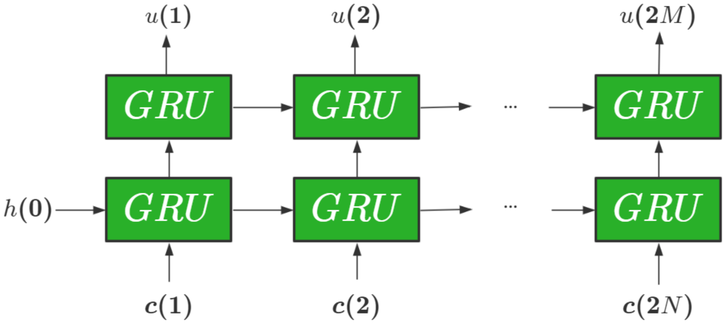
At first, the neural network is a two-layer recurrent neural network. It takes the far-field data
as the input, the information parameter
as the output, and the GRU gate control unit as the basic computing unit. The neural network is used for the reconstruction of the information parameter
. Its structure is shown in
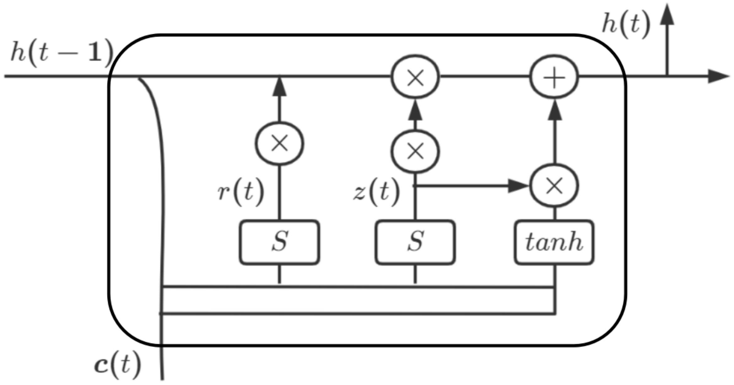
Figure 2. The rectangle represents the GRU gate control unit, and its structure is shown in
Figure 3.
Given the input
and the initial state
, after the calculation of the first layer of GRU gate control unit, the far-field feature
h is obtained
where
and
represent the feature of the
tth and
th components of the far-field data, respectively. When
,
has no far-field feature. The calculation process of the GRU gate control unit is as follows:
(1) Reset gate
determines how the input information
is combined with the previous feature
,
at this point, the candidate feature
is
(2) The update gate
determines the information to be retained by the current feature
from the historical feature
, and the new information
to be added from the candidate feature
and computes the intermediate feature
The intermediate feature
represents the feature extracted from the first layer of the hidden layer of the neural network. To further improve the accuracy of the solver, the hidden layer adds another layer of the GRU unit for feature extraction. Input
and intermediate feature
into the GRU unit (9)–(12) for calculations to obtain the final feature
The output
of the module can be expressed as
where
is a sigmoid activation function,
is the hyperbolic tangent activation function,
can be any activation function,
,
,
,
are the weight of the reset gate, the intermediate state, the update gate, and the output layer, respectively, ⊗ denotes the matrix corresponding element multiplication, and ⊕ denotes the matrix splicing.
Here, the loss generated by the data-driven module can be represented by
and
as
2.3. Physical-Driven Module
In the previous section, we considered the loss between data , and . In this section, we will continue to consider the relationship between far-field data and the information parameter of the source. From a physical point of view, the output of the data-driven module is the result of the reconstruction of the information parameter. So, the information parameter represented by should meet the Lamé system. If will be substituted into the Lamé system, the corresponding far-field data will be obtained. Then the loss between the far-field data of reconstruction and the real far-field data will be considered. In this way, we can evaluate the results of solver reconstruction from both data-driven and physical-driven aspects.
The physical model satisfied by the elastic wave field
is the Lamé system:
where
,
are the Lamé constant, satisfying
,
, and
is the angular frequency of the elastic wave,
is the Dirac distribution,
is the magnitude of the
jth source,
is the location of the
jth source, and
N is the number of point sources. From the discussion in the introduction, we study the correspondence between the information parameter of the source and the far-field, and take the Formulas (4) and (5) instead of the Lamé system.
We use the data-driven module to calculate
and substitute it into the Formulas (4) and (5). The far-field data
can be expressed as
where
represents the location of the
jth source of the reconstruction,
represents the magnitude of the
jth source of the reconstruction,
,
is the unit matrix,
represents the observation direction, and
i represents the imaginary unit.
At this time, the loss generated by the physical-driven module with
as the input, and
as the output can be expressed as
2.4. Loss Function of the DDS
In this section, we define the form of loss function for the dual-driven solver.
Based on the loss (13) of the data-driven module and the loss (17) of the physical-driven module, the loss function of the dual-drive solver can be defined as
where
is the loss of the data-driven part,
is the loss of the physical-driven part, and
is the contribution coefficient of the physical-driven model,
. When
, the dual-driven solver is a two-layer GRU neural network driven by data. Through the definition of the loss function (18), the loss of physical-driven module is added to the loss function of the training neural network. It directly affects the optimization of the network weights and acts as a regularization in DDS.
For the DDS, the Adam algorithm is used to update the weights in the data-driven module to update the solver.
W is used to represent the weight
in the solver. The weight update rules are as follows.
where
represents the random initial weight,
represents the value of the parameter
W at
l iterations,
,
is a constant added to maintain numerical stability,
is the learning rate,
is the correction of
, and
is the correction of
,
and
are constants to control the exponential attenuation.
is the exponential moving mean of the gradient, which is obtained by the first-order moment of the gradient.
is the square gradient, which is obtained by the second-order moment of the gradient. The updates of
and
are as follows
represents the value of the loss function
L at
l iterations,
is the gradient matrix obtained by the derivative of the loss function
L with respect to the weight
W.
Finally, we give the reconstruction scheme in the following Algorithm 1.
| Algorithm 1 A numerical method for reconstructing the source from far-field data |
- Step 1
Given the frequency , , and information parameter , calculate the corresponding far-field data ; - Step 2
Enter the far-field data into the DDS; - Step 3
The data-driven module reconstructs the parameter and calculates module losses (13); - Step 4
Enter into the physical-driven module to get () and calculate module loss (17); - Step 5
Calculate DDS loss using module loss (18) in Step 3 and Step 4; - Step 6
Determine or achieve the maximum number of iterations: Yes, continue to Step 7; No, use the Adam algorithm to update the weight, and then return to Step 2; - Step 7
DDS outputs parameter .
|
3. Numerical Experiments
Through the numerical experiments, this section shows that the constructed DDS can effectively reconstruct the location and magnitude of the source. In addition, several two-dimensional and three-dimensional numerical experiments are used to illustrate the effectiveness and robustness of DDS.
In all numerical examples, we consider the , and Lamé constants , . For two-dimensional cases, we select a circle with a radius of as the measurement curve , and evenly distribute 10 measurement points counterclockwise from the x-axis on . For three-dimensional cases, we chose 100 uniformly distributed measurement directions on the sphere with a radius of .
Experiment 1. Selection of hyperparameters of the data-driven module in DDS.
In this experiment, we consider the value of the maximum number of iterations in the neural network.
Figure 4 shows the curve of the test loss function changing with the number of iterations. It can be seen from the figure that when
Iterations
, the test loss decreases with the increase of the number of iterations and changes significantly. When
Iterations
, the test loss decreases slightly with the increase of the iterations. When
Iterations, the test loss hardly changes. This means that the maximum number of iterations in the network is 400. This way, better results are obtained without wasting the calculation cost.
Some parameters of the data-driven module in DDS are set in the
Table 1. More details on parameter settings can refer to Refs. [
27,
29,
32].
Experiment 2. Reconstruction of the location and magnitude of the single source.
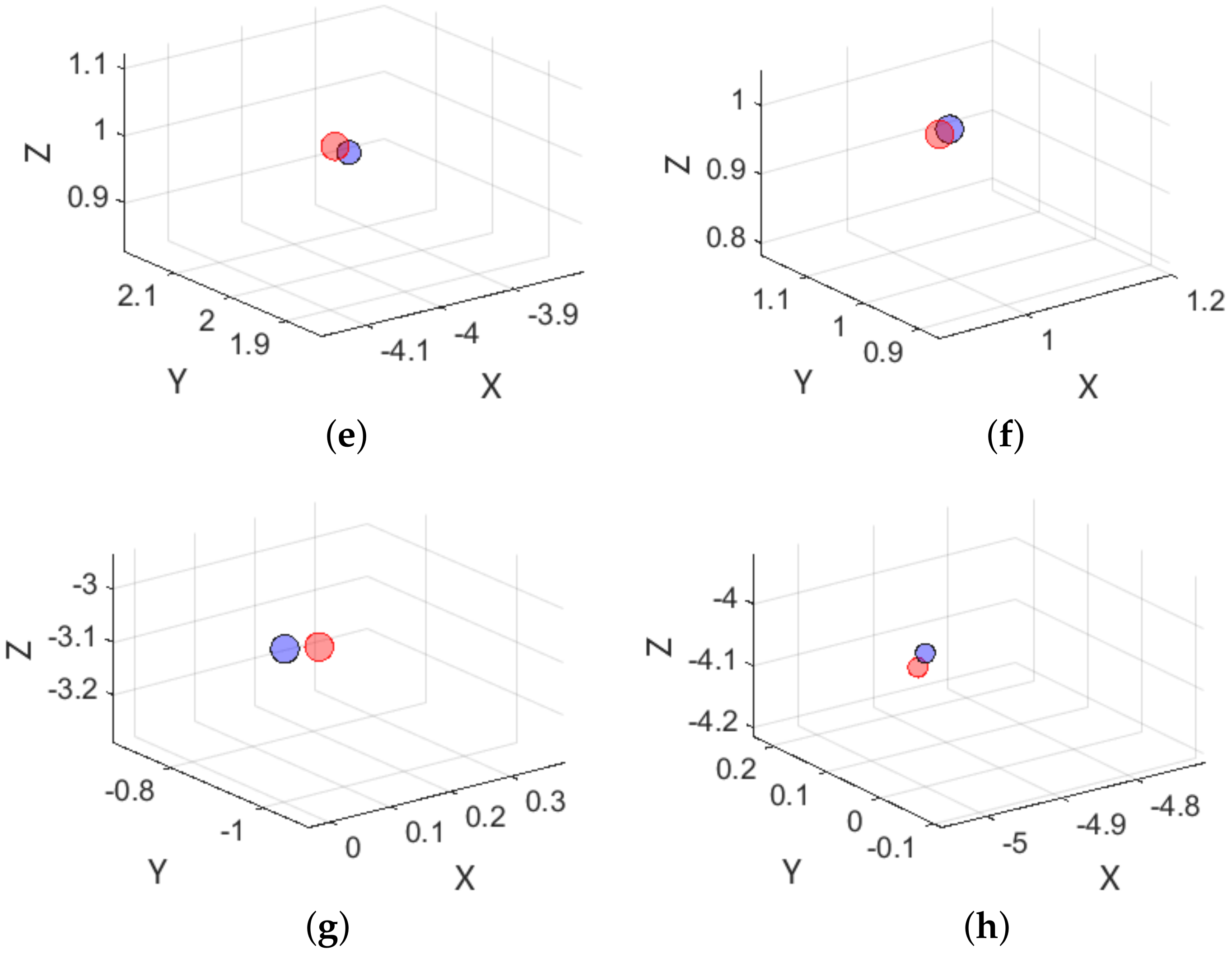
In this experiment, we consider far-field data to reconstruct the location and magnitude of a single source in two-dimensional and three-dimensional cases, respectively. The calculation results are shown in
Figure 5.
Figure 5 shows the reconstruction results of the location and magnitude of a single source in 2D and 3D. Compared with the two adjacent dots of different colors in the figure, we find that the location and size of the dots are basically the same. It shows that the solver can reconstruct the location and magnitude of the source in 2D and 3D. In order to quantitatively observe the accuracy, we give the information parameter of the refactoring source and the relative error between the two in
Table 2 and
Table 3, respectively.
As can be seen from
Table 2 and
Table 3, there are discrepancies between the refactored parameters of location and magnitude, but the actual values are similar, indicating that the solver can not only invert the position and strength information of the point source simultaneously, but also that the accuracy is consistent.
In the two-dimensional and three-dimensional reconstruction experiments, the relative errors of each group are different. The main reason is the random generation of weight initialization in the neural network and the decrease of the stochastic gradient in the optimization algorithm. It makes the data-driven module have a certain degree of randomness. At the same time, we can see from
Table 1 that the maximum number of iterations of the solver is 400. This means that the solver will terminate and output the reconstruction results at this time, when the number of iterations reaches 400. A subsequent number of iterations will perhaps get better reconstruction results. However, the solver will only output the inversion results when the number of iterations is terminated. Combined with the above reasons, each reconstruction result will be different and the error will vary.
Least-squares method is widely used in underground scattering imaging. Let us do a comparative experiment. Using least-squares [
43] to reconstruct the single source under the same data volume, the results can be seen in the
Table 4. Comparing the
Table 2 and
Table 4, it can be seen that the reconstruction effect of the DDS is stronger than the least-squares.
From Experiment 2, it can be seen that the solver can solve the inverse source problem in 2D and 3D. Additionally, there were no inherent concerns in the solution process. Therefore, the subsequent experiments are considered in 2D.
Experiment 3. Reconstruction of the number of multi-sources.
In this experiment, our goal is to reconstruct the number of the point sources. The information parameter of the source is shown in
Table 5. On account of the number of information, the parameter in our method must be determined before reconstruction, that is, the number of point sources must be known. In the case of an unknown number, let us first move
and
in a certain direction so that the location
is not in
. Secondly, it is assumed that the number of sources is
Q, which requires
. Then we use the solver to reconstruct the location of the source. If the location
of
q point sources is reconstructed. It means that the
q point sources does not exist, and the number of sources is
.
Table 5 shows the reconstruction of the number of two point sources. Since the number of sources is unknown in advance, we assume that there are three sources. Through the reconstruction results of
Table 5, we can see that the reconstruction location parameter of point source
is
, indicating that point source
does not exist. This means that the number of multi-sources is two, which is consistent with the actual number of the point sources. Therefore, this method of refactoring the number of sources is feasible. At the same time, the location parameters of the reconstruction can be seen through the value of relative error.
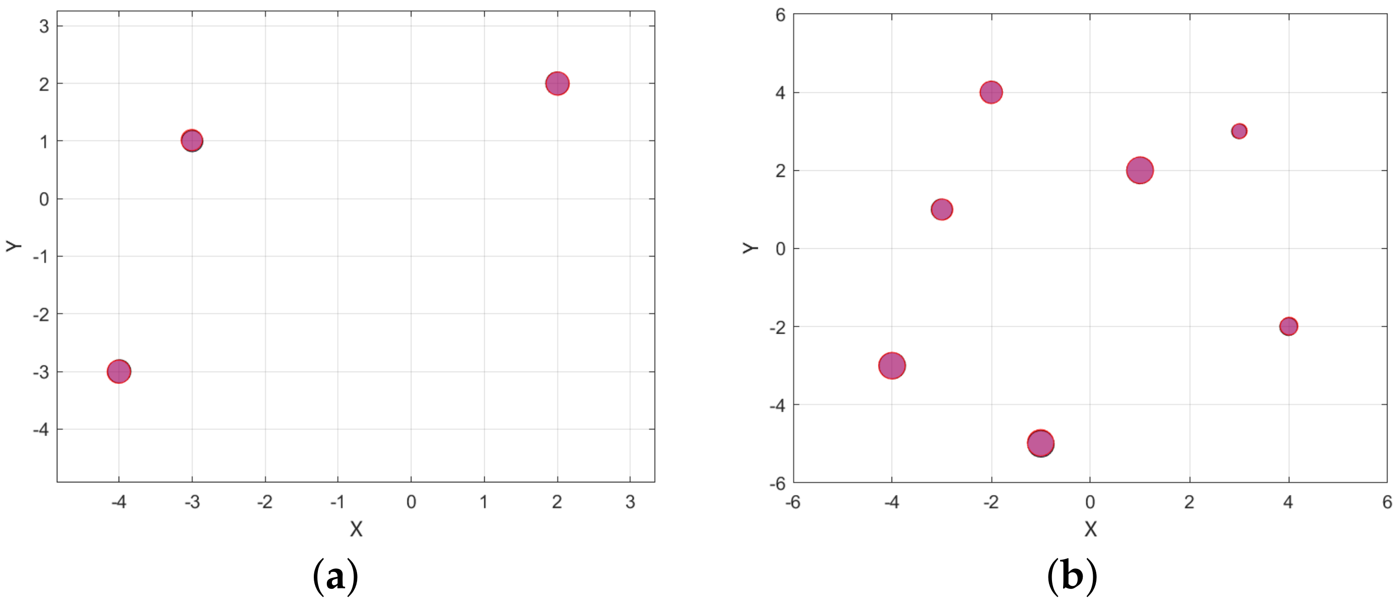
Experiment 4. Reconstruction of the location and magnitude of multi-sources.
This experiment considers reconstructing the location and magnitude of multi-sources in different locations when the number of sources is known. In
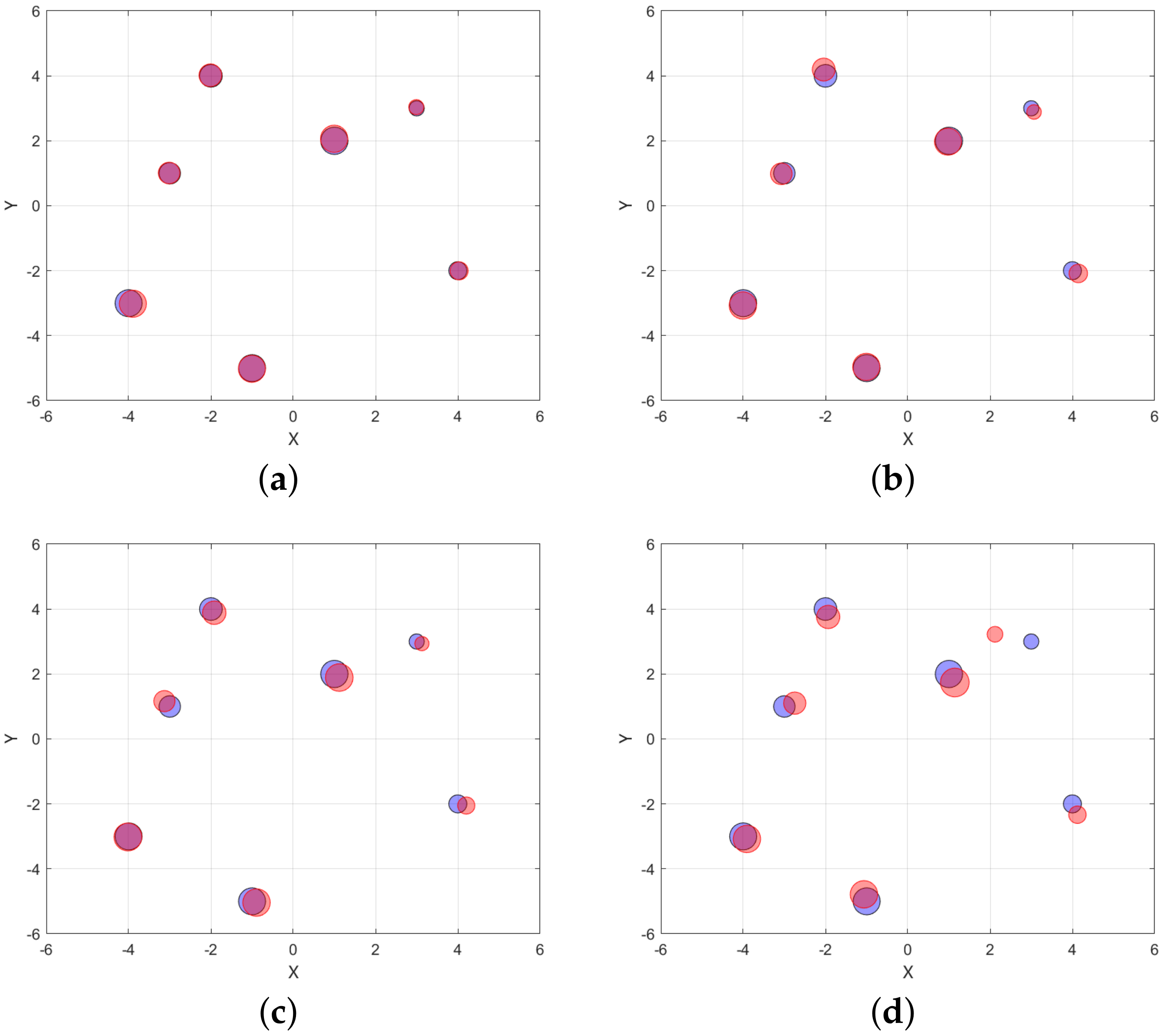
Figure 6, we rebuild three and seven point sources, respectively.
In
Figure 6, the reconstructed red dot has a good coverage of the real blue dot, which means that the reconstruction results are good. In order to accurately see the results of the reconstruction,
Table 6 and
Table 7 give the number, location, and magnitude parameter information of real and reconstructed sources. Comparing the relative error range of
Table 6 and
Table 7, we can see that the increase in the number of point sources does not affect the accuracy of the results.
In
Figure 7, we present the waveform plots generated by the true and reconstructed scattering fields from three point sources. The circle ring represents the PML layer.
Experiment 5. Reconstruction of the point sources under different noise levels.
In this experiment, different levels of noise are added to the measurement data of the point sources to test the stability of the solver. We add some random disturbances to the data, and the noise data is expressed as
where
represents the level of noise, and
is a random number generated by a uniform distribution
. We add 1%, 5%, 10%, and 20% respectively, to the training dataset.
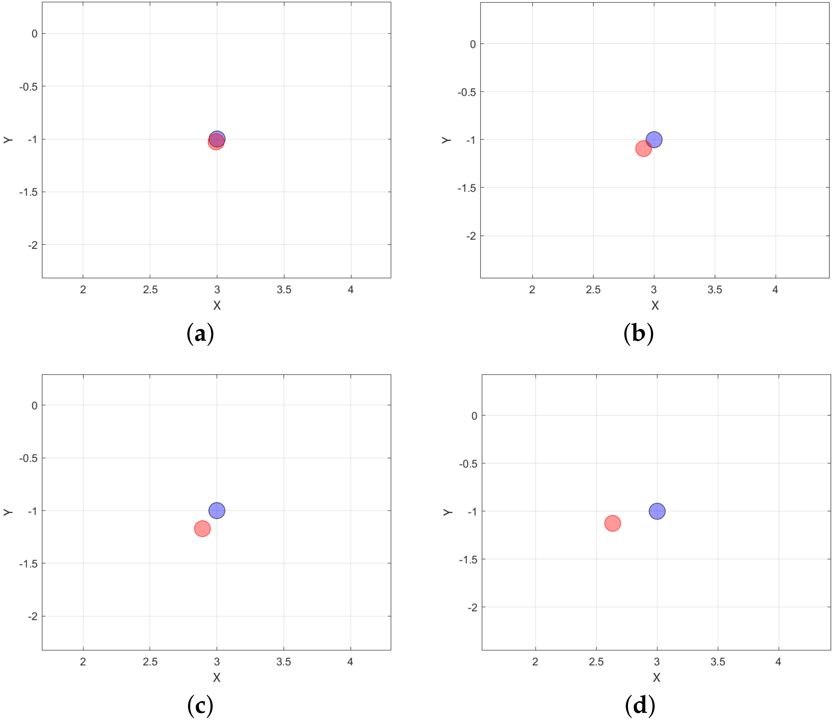
Table 8 shows the reconstruction results of one point source with location (3, 2) and magnitude (5, −7) at different noise levels. From it, we can plainly observe that the reconstruction results gradually deteriorate and the relative error increases as the noise level rises. This can also be verified in
Figure 8. The distance between the reconstruction location and the exact location increases with the noise intensity. It has no discernible effect on the results when less than 5% noise is added. The location of the reconstruction significantly deviates from the genuine place as the noise level rises above 10%.
Figure 9 shows the reconstruction of seven point sources at different noise levels. The above view can also be demonstrated in
Figure 9. In addition, we also find that with the increase in noise level, the reconstruction effect of large dots is significantly stronger than small dots. This may be caused by the observation point capturing too little information with the small magnitude of the point. In order to intuitively feel the error of each point, we give the relative error of each point at different noise levels and the average error of this set of points in
Table 9.
Experiment 6. Reconstruction of point sources under finite observation apertures.
In actual applications, full-aperture measurement of far-field data is often limited and can only be collected at limited observation points. It means that the observation geometry is only partial. This experiment considers reconstructing the location and magnitude of single point and multi-sources under finite observation apertures. This enables a thorough evaluation of the solver’s stability. We select the observation aperture ranges of , , and respectively, and the corresponding number of observation points is , , and .
The reconstruction renderings of a single source and multi-sources in different observation aperture ranges are shown in
Figure 10 and
Figure 11, respectively. They clearly show that with the reduction of the observation aperture range, the reconstruction effect gradually deteriorates. In the reconstruction of multi-sources, when the observation aperture reduces to
, the reconstruction results have a small impact. When the observation aperture is
, the observation point captures more information about the nearby points, and the reconstruction results of the point on one side of the observation point is better than the other side. When the observation aperture is
, the observation point that collects the information is seriously insufficient, and the reconstruction location seriously deviates from the real location.


