
Stability Analysis of the Inhomogeneous Perturbed Einstein Universe in Energy–Momentum Squared Gravity


Department of Mathematics and Statistics, The University of Lahore, 1-KM Defence Road, Lahore 54770, Pakistan
*
Author to whom correspondence should be addressed.
Universe 2023, 9(3), 145; https://doi.org/10.3390/universe9030145
Submission received: 6 February 2023
/
Revised: 28 February 2023
/
Accepted: 9 March 2023
/
Published: 10 March 2023
(This article belongs to the Section Cosmology)
Abstract
:The main objective of this article is to examine the stability of Einstein static universe using inhomogeneous perturbations in the context of energy–momentum squared gravity. For this purpose, we used FRW spacetime with perfect matter distribution and formulated static as well as perturbed field equations. We took a minimal model of this theory to investigate the stable regions of the Einstein universe for conserved and non-conserved energy–momentum tensors. We found that stable modes of the Einstein universe appeared in both conserved and non-conserved cases for all values of the equation of state and model parameters corresponding to both open and closed cosmic models. We found that stable solutions in this modified theory were obtained for a broader -region compared to other modified theories.
1. Introduction
Cosmic expansion was a most astonishing and spectacular discovery for the scientific community [1,2,3]. Although general relativity (GR) is a widely accepted theory that explains the cause of this expansion, it has two major flaws: coincidence and fine tuning problems. To address these issues, several modifications of GR (modified gravitational theories) have been established to unveil cosmic mysteries. The simplest modified theory is gravity. A significant body of literature [4,5,6] is available to aid in the understanding of the physical features of this theory. The concept of coupling between geometric and matter parts has gained the attention of many researchers in recent years. These are non-conserved theories that ensure the presence of an extra force and, consequently, the non-geodesic motion of particles [7,8,9,10,11,12].
The presence of singularities is considered a major problem in GR because of their prediction at the high energy level, where GR is no longer valid due to the expected quantum impacts. However, there is no specific formalism for quantum gravity. In this regard, a new generalization of GR was recently proposed, which allows a correction term in the functional action, which is known as energy–momentum squared gravity (EMSG). This is also referred to as theory, where is denoted by [13]. Moreover, this theory is equivalent to GR in a vacuum. This modification of GR is considered the most favorable and prosperous technique that resolves the spacetime singularity in the non-quantum description. Consequently, the corresponding field equations are different from GR only in the presence of a matter source. It contributes squared terms to the field equations that are used to explore various fascinating cosmological consequences. It is worthwhile mentioning here that this theory overcomes the spacetime singularity but does not change the cosmic evolution.
Energy–momentum squared gravity is a cosmological model where the scale factor is non-vanishing at all times and, hence, does not favor big-bang cosmology. However, the profile of density in the radiation-dominated universe shows that EMSG supports inflationary cosmology. Inflationary cosmological models are successful in providing convincing answers to major cosmological issues, such as the horizon problem and the flatness problem, but no model of inflation has observationally been confirmed. In this perspective, varying terms in the speed of light theories were introduced, which are a class of cosmological models that disfavor inflation. These proposed an alternative route to solve these cosmological issues by just allowing the speed of light and the Newtonian gravitational constant to vary. Varying terms in the speed of light theories were introduced to address the shortcomings of inflation, but did not address the shortcomings related to the initial big-bang singularity. To address this issue, Bhattacharjee and Sahoo [14] presented a novel cosmological model that was free from both the initial big-bang singularity and inflation by incorporating varying speed of light and Newtonian gravitational constant terms in the framework of EMSG. Singh et al. [15] studied the viability and stability of color-flavor locked quark stars in this framework. Nazari [16] studied the behavior of light rays in the weak-field limit of EMSG and found that this theory passed the solar system tests. It was revealed that except for a small deviation, the overall behavior of EMSG light curves was similar to that in GR.
The existence of the term induces some quadratic corrections to the Friedman equations that are reminiscent of the corrections reported in the context of loop quantum gravity [17]. Board and Barrow [18] found a range of exact solutions for the isotropic universe and discussed their behavior with reference to early and late time evolution, accelerated expansion and the presence or absence of singularities. Akarsu et al. [19] proposed a modified theory of gravitation that was constructed by the addition of the term to the Einstein–Hilbert action, and they elaborated a particular case, , where and are real constants, dubbed as energy–momentum powered gravity. They discussed that this modified theory could be unified with Starobinsky gravity to describe the complete history of the universe, including the inflationary era. Akarsu et al. [20] introduced a scale-independent EMSG that allowed different gravitational couplings for different types of sources, which might lead to scenarios with many interesting applications in cosmology. Ranjit et al. [21] examined possible solutions for matter density and discussed their cosmological results in EMSG. Sharif and Naz [22] studied physical characteristics of a gravastar in this framework.
Chen and Chen [23] investigated the axial perturbations of charged black holes in this theory. It is important to mention here that EMSG was not limited to the early universe and bouncing solutions. For instance, this model was used to manipulate cosmic microwave background quadrupole temperature fluctuation [24]. Kazemi et al. [25] studied the local gravitational stability of an infinite fluid (Jeans analysis) and a differentially rotating fluid disk (Toomre criterion) in the context of EMSG. Rudra and Pourhassan [26] explored the thermodynamic properties of a black hole in the background of EMSG. Nazari et al. [27] studied the Palatini formulation of EMSG and explored its consequences in different contexts. We examined the exact solutions through Noether symmetry approach [28,29,30,31,32,33], dynamics of gravitational collapse [34,35,36,37,38] and geometry of compact stars [39,40,41] in this framework. Yousaf et al. [42] investigated the effects of gravity on the dynamical evolution of axially and reflection symmetric anisotropic and dissipative fluid. They found that modified scalar variables bearing the effects of electric and magnetic components of the Weyl tensor played a vital role in the evolution of compact objects. Khodadi and Firouzjaee [43] used linear perturbations due to the massless scalar field in Reissner–Nordstrom–de Sitter solutions in this framework, and they developed the valid study of strong cosmic censorship conjecture beyond Einstein’s gravity.
Initially, it was assumed that the entire matter was compressed to an infinitely dense point known as the big-bang or primordial singularity. This is the most crucial issue in the field of cosmology. Different strategies for developing non-singular cosmic models have been proposed to tackle this issue. In this regard, the emergent cosmos has been developed that resolves the primordial singularity. According to this scenario, the initial state of the cosmos is an Einstein static universe (ESU) rather than a primordial singularity. The emergent scenario is a successful one to describe a singularity-free universe, provided that it satisfies two conditions at the same time: stable Einstein static solutions can be found in it and a graceful exit from it to inflation is possible. However, this cosmos was not adequately demonstrated in GR because of unstable solutions. Analysis also showed that ESU remained stable against inhomogeneous perturbations when the speed of sound, , satisfied the condition [44]. The stability of the ESU with isotropic/anisotropic fluid configuration was investigated in [45] and unstable modes corresponding to homogeneous perturbations were found.
Barrow et al. [46] analyzed the stability of the Einstein static universe (ESU) against inhomogeneous vector and tensor perturbations and found that ESU was stable if the square of the speed of sound was greater than 1/5, otherwise it was unstable. Canonico and Parisi [47] investigated the existence of static solutions in the framework of the loop quantum gravity model, and they showed that the presence of a negative curvature index increased the stable modes of the solutions. Wu and Yu [48] studied the stability of the ESU with respect to Horava–Lifshitz gravity, and they found that a stable Einstein static state existed if the cosmological constant was negative. Atazadeh and Darabi [49] explored the stability of the ESU using the FLRW metric against linear homogeneous perturbations in kinetic coupled gravity. They found that the stability of the ESU for the closed universe model depended on the coupling parameters. Mohsen et al. [50] found the ESU solutions and examined their stability through phase space analysis. Ilyas et al. [51] presented an emergent universe scenario by introducing a deformed kinetic term and degenerated a higher-order scalar–tensor coupling into the original Galileon Genesis model. They showed that the universe could exit the emergent phase and transfer to a radiation-dominated phase.
Khodadi et al. [52] examined the effects of rainbow gravity on the stability of the Einstein static state against homogeneous scalar, vector and tensor perturbations. They showed that in the presence and absence of an energy-dependent cosmological constant, a stable Einstein static solution existed against homogeneous scalar perturbations. Heydarzade et al. [53] investigated the stability of the Einstein static state against homogeneous scalar, vector and tensor perturbations in the framework of Horava–Lifshitz gravity. It was shown that there was no stable ESU for the flat universe model. Li and Wei [54] studied the stability of the ESU filled with perfect fluid against homogeneous and inhomogeneous scalar perturbations in the Eddington-inspired Born–Infeld theory. They found that the ESU against scalar perturbations in both flat and closed cases was not stable. Mousavi and Darabi [55] studied static cosmological solutions and their stability in the framework of massive bigravity theory. They found that the obtained solutions for closed and open universe models were stable for specific values of the equation of state parameter. Sarkar and Das [56] used the equation of state parameter to explore the emerging universe in non-linear electrodynamics.
Bohmer et al. [57] investigated the stability of static solutions against homogeneous and inhomogeneous perturbations in the framework of scalar–fluid theory. They found that stable solutions existed against inhomogeneous perturbations, but homogeneous perturbations yielded unstable solutions. Khodadi et al. [58] investigated the ESU and the emergent universe scenario in the framework of gravity. They performed a dynamical analysis in the phase space and showed that stable static phase existed corresponding to the open universe model. Li et al. [59] showed that the stable regions of the ESU against homogeneous and inhomogeneous scalar perturbations existed in Gauss–Bonnet gravity. Huang et al. [60] analyzed the stability of the ESU against scalar perturbations in the mimetic theory and found that stable solutions existed under certain conditions. Khodadi et al. [61] studied the emergent universe scenario in the context of EMSG and found that it was possible to remove the initial singularity with some favorable conditions, as well as in the absence of quantum corrections.
The stability of the ESU was studied in [62] by using homogeneous perturbations in theory. The stability of the ESU through an EoS in modified Gauss–Bonnet gravity was analyzed in [63]. The stable regions of the ESU were explored in gravity, which were not stable in theory [64]. Sharif et al. [65,66,67,68,69,70] analyzed the stability of the ESU against homogeneous/inhomogeneous and isotropic/anisotropic perturbations with different matter configurations in minimal and non-minimal curvature–matter coupled theories. They also analyzed their solutions graphically and compared them with the current literature. Recently, we explored the stable modes of the ESU by applying homogeneous perturbations in theory and found that stable regions existed for entire values of the EoS variable [71,72].
This paper examines the stability of the ESU against inhomogeneous perturbations in the background of EMSG. This analysis would be useful to investigate the impact of modified theory and inhomogeneous perturbations on the stability of the ESU. The paper is arranged as follows. Section 2 establishes the field equations of the static ESU. A detailed study of inhomogeneous perturbations is given in Section 3. The stable regions of ESU modes for both conserved and non-conserved energy-momentum tensors (EMTs) are examined in Section 4. The summary of the obtained results is given in Section 5.
2. Einstein Universe
In this section, we establish the field equations of the FRW universe with an isotropic matter distribution in the context of EMSG. The action of this modified theory is determined as [13]
where and manifest the coupling constant and Lagrangian of matter, respectively. By varying the action corresponding to , we have
Solving the above equation, we obtain
where . Here, we have used the relation . The energy–momentum tensor is defined as
Assuming that the Lagrangian of matter depends only on the components of the metric tensor, and not on their derivatives, we have
The variation of the Ricci scalar is given by
For the variation of , we have
Now, using Equation (4), we have
In the above expression, we have used the relation (where symbolizes the generalized Kronecker delta). We can write
where T is the trace of the energy–momentum tensor. For the sake of our convenience, we denote by . Consequently, we have
which shows that depends on the Lagrangian of matter explicitly. Using the values of and in Equation (2), the field equations for gravity turn out to be
The EMT determines the distribution of matter and energy in the system and every non-vanishing element yields a dynamical variable with some physical attributes. The isotropic matter configuration is assumed to be
where four-velocity, energy density and pressure of the fluid are determined by , and p, respectively. If the Lagrangian of matter is of second or higher order in the metric then the second derivative of the Lagrangian of matter with respect to the metric is non-zero. Thus, for a perfect fluid, the term can be dropped. We have considered the Lagrangian of matter, , as this choice has already been used in literature [73]. Therefore, Equation (8) reduces to
Using Equation (10) in (11), we have
Rearranging Equation (9), we obtain
where defines the additional effects of EMSG, represented as
The non-conservation equation of this theory is given by
We consider FRW spacetime to analyze the homogeneous and isotopic universe as
Here, represents the conformal scale parameter, whereas K defines the spatial curvature variable that yields flat , open and closed cosmic geometries. The resulting field equations are
where a dot represents the rate of change with respect to time, while corresponding values of R and become
The query about the initial cosmic state has offered fascinating results over the last few decades. According to Einstein’s equations of motion, the current expansion of the universe must be preceded by a singularity, where the physical laws break down. To resolve this issue, the emergent cosmic scenario was developed, which overcame the primordial singularity. This universe has interesting features, such as no initial singularity, an ever-existing universe and static behavior in the infinite past. The main motivation behind developing this technique was to examine the existence of a stable ESU. The ESU’s solutions must be stable in the face of any perturbations so that the cosmos might continue to exist in a static condition. We assume that to examine the static ESU. The corresponding equations of motion turn out to be
where and .
3. Inhomogeneous Scalar Perturbations
The perturbation approach is an extremely effective technique that reduces the complexity of a physical system. There are various types of perturbations, including isotropic, anisotropic, homogeneous and inhomogeneous perturbations. Several researchers have used these perturbations to examine the stable regions of the ESU. The stable modes of the ESU using inhomogeneous perturbations do not exist in theory [74]. What will occur in the background of EMSG? Will the stability of the ESU appear against inhomogeneous perturbations? To find the answers to these queries, we examined the stability of the ESU in theory. We assume perturbed spacetime to be [75]
where defines the Bardeen potential and is the perturbation to spatial curvature. The scalar perturbations in fluid variables become
where the perturbed pressure and energy density are represented by and , respectively. The harmonic decomposition of inhomogeneous perturbations is expressed as
where demonstrates the spatial coordinates when summation on is considered. The harmonic function for distinct cosmic geometries satisfies the following relations:
where the Laplacian operator is denoted by .
These inhomogeneous perturbations provide a continuous spectrum for flat and closed universe models, whereas a discrete spectrum is obtained for the open cosmic model [74]. It was noted that linear homogeneous perturbations were recovered for . By using inhomogeneous perturbations and Taylor series expansion, we have
Here is the EoS variable. The linearized and diagonal components of perturbed spacetime (20) yield the following:
The non-diagonal elements with perfect fluid yield the following relation:
which does not satisfy the anisotropic matter configuration. The perturbed field equations, Equations (22) and (23), helped to investigate the stable modes of the ESU but these equations are in complex form.
To investigate the stability of the ESU in EMSG, we took a particular form of a generic function that yielded minimal interaction between curvature and matter parts:
The corresponding field equations with respect to the minimal model (25) turned out to be
where prime is the rate of change with respect to , i.e., or . Eliminating , and from Equations (26) and (27), we have
Manipulating Equations (18) and (19), we obtain
Substituting the value of into Equation (28), the required perturbed field equation in terms of is
The presence of stable regions in the ESU for particular values of and are examined in the following section.
4. Stability Analysis
In this section, we analyze solutions of the ESU with . Firstly, we perturb the non-conservation equation and examine the stable modes graphically. Secondly, we consider the specific form of to investigate the stability of the ESU.
4.1. Case I
The non-conservation equation of FRW spacetime with perfect matter distribution is
The resulting second-order differential equation corresponding to the model (25) is
The solution of this equation is
where and are integration constants. Inserting Equation (25) into the above, with in (22), the corresponding perturbed equation becomes
where
where and is the frequency of a small perturbation given by
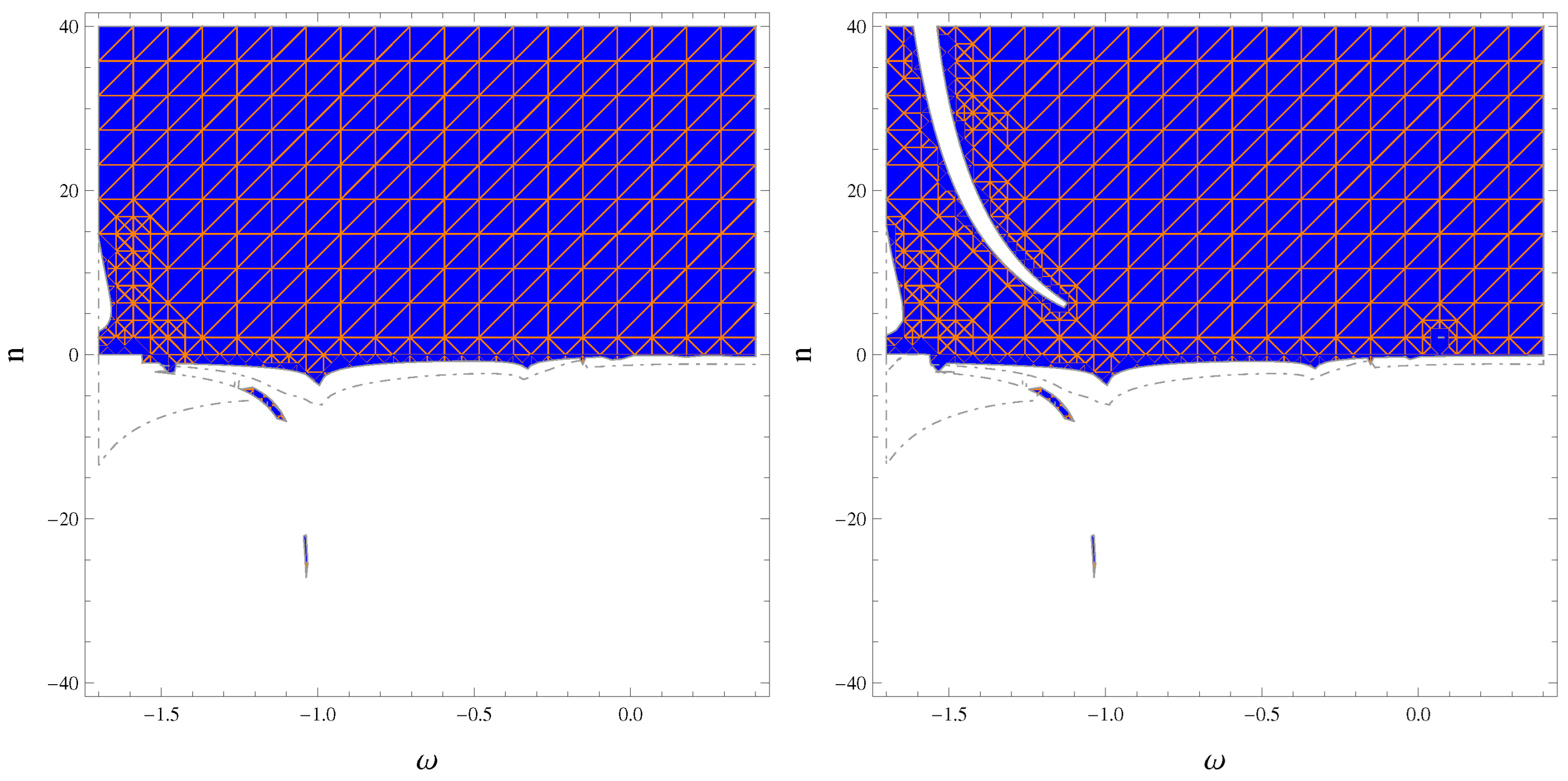
The presence of stable and unstable modes of the ESU depends only on the exponential growth of perturbations. The inequality yields stable solutions, whereas unstable ones exist for . We considered the current value of as [76] to analyze the stable modes of the ESU graphically. Figure 1 shows the existence of as well as stable modes of the ESU for closed and open cosmic models corresponding to various values of . In the right plot, the blue color indicates the regions for and the orange color represents the region for , whereas blue and orange colors in the left plot indicate the regions for and , respectively. The stability of the system is represented by the common regions. Figure 1 shows that the stability of the ESU increased with an increasing value of the integration constant for the closed universe model, while stability of the ESU decreased with an increasing value of the integration constant for the open universe model. However, in both cases, the existence of the ESU was acquired for all values of . From these graphical analyses, we observed that the stability of the ESU against inhomogeneous perturbations increased compared to homogeneous perturbations in EMSG [72]. In the conserved EMT case, it was found that for no stable region existed for positive as well as negative values of in theory [66]. While in theory, it was shown that the stable ESU existed only for [67]. We found stable modes of the ESU, which were not stable in other gravitational theories [65,66,67,68,69,70].
4.2. Case II
We examined the stable modes of the ESU for non-conserved EMT. For this purpose, we assumed [18,20]
to investigate the effects of non-conserved EMTs on the stability of the ESU. Here, is an arbitrary constant. The solution of Equation (33) corresponding to this model gives the frequency of small perturbation as
where
The frequency of a small perturbation turns out to be
The graphical interpretation of stable regions against inhomogeneous perturbations in the non-conserved case for different values of and is given in Figure 2, Figure 3, Figure 4 and Figure 5. Figure 2 and Figure 3 correspond to the closed universe model, while Figure 4 and Figure 5 correspond to the open cosmic model. For the closed cosmic model, we found that stability increased for positive values of n and , while it decreased for negative values of . For the open cosmic model, the stable regions of the ESU existed only for positive values of n. We found that stable modes existed for all values of , and these stable regions became more smooth as increased in the open universe model and decreased in the closed universe model. However, more stable regions existed in the closed universe model compared to the open universe model. For non-conserved EMT, stable regions were observed only for negative values of the EoS parameter in the framework of theory [66], while the stability decreased with a decreasing value of the model parameter in gravity [67].
5. Final Remarks
The stability of the EU is considered the most debatable problem in cosmology. Einstein tried to find a static solution of the field equations to describe the isotropic and homogeneous universe. Since the field equations of GR have no static solution, Einstein, therefore, introduced the term known as the cosmological constant in order to have static solutions. It is important to know whether it can provide a natural initial state for a past eternal universe, whether it allows the universe to evolve away from this state and whether, under any circumstances, it can act as an attractor for the very early evolution of the universe. With these questions in mind, we have investigated in detail whether the EU is stable or unstable against linear inhomogeneous perturbations.
One of the most fundamental issues in cosmology is the mystery behind the beginning, as well as origin, of the universe. According to some physical constraints on cosmic matter configuration, GR equations suggest that the current expanding cosmos must have been preceded by a singularity known as the big-bang singularity, where the physical parameters, such as energy density and spacetime curvature diverged. The emergent universe scenario is based on the pillars of the stable EU and is considered a favorable approach in cosmology to resolve the captivating issue of a primordial singularity. The initial state of the universe in this framework is the EU, instead of a primordial singularity, which then smoothly evolved into the rapid exponential inflationary era [77,78]. This conjecture implies that the initial cosmic epoch was the EU, which entered into an expanding posture that led to the inflationary phase. The phenomenon of the EU is mainly manifested by the closed FLRW universe with isotropic fluid and the cosmological constant. The most essential characteristic of a successful emergent universe depends upon the stable solutions of the EU for any type of perturbation.
In this paper, we examined the stable zones of the ESU against inhomogenous perturbations in EMSG. This modified theory is non-conserved because of coupling between curvature and matter parts. We formulated field equations for the static and perturbed system through a barotropic EoS. We considered the minimal EMSG model to construct the perturbed equations whose solutions helped to analyze the stable modes of the ESU. For the considered model, we examined the conserved/non-conserved EMT cases against the inhomogeneous perturbations. The major results are given as follows.
- A unique expression of for the conserved EMT case was developed that satisfies the conservation equation. We investigated the stable modes of the ESU against for distinct values of . It was found that stability of the ESU existed for all values of corresponding to closed and open cosmic models.
- We assumed a particular type of in the non-conserved case and analyzed the stability of the ESU for different values of . We found that stable modes existed for entire values of . These stable regions became more smooth as the model parameter increased in the open universe model and decreased in the closed universe model. It is worthwhile to mention here that our solutions reduced to homogeneous perturbations for .
We note that stable solutions covered a broader -region, while other theories were comparably limited.
Author Contributions
M.S. proposed the problem, supervision and finalized the paper while M.Z.G. did the calculations and prepared the draft. All authors have read and agreed to the published version of the manuscript.
Funding
This research received no external funding.
Data Availability Statement
No new data were generated or analyzed in support of this research.
Conflicts of Interest
The authors declare no conflict of interest.
References
- Perlmutter, S.; Aldering, G.; Deustua, S.; Fabbro, S.; Goldhaber, G.; Groom, D.E.; Kim, A.G.; Kim, M.Y.; Knop, R.A.; Nugent, P.; et al. Cosmology from type Ia supernovae. Bull. Am. Astron. Soc. 1998, 29, 1351. [Google Scholar]
- Filippenko, A.V.; Riess, A.G. Results from the high-z supernova search team. Phys. Rep. 1998, 307, 31. [Google Scholar] [CrossRef] [Green Version]
- Tegmark, M.; Strauss, M.A.; Blanton, M.R.; Abazajian, K.; Dodelson, S.; Sandvik, H.; Wang, X.; Weinberg, D.H.; Zehavi, I.; Bahcall, N.A.; et al. Cosmological parameters from SDSS and WMAP. Phys. Rev. D 2004, 69, 103501. [Google Scholar] [CrossRef] [Green Version]
- Cognola, G.; Elizalde, E.; Nojiri, S.; Odintsov, S.D.; Sebastiani, L.; Zerbini, S. Class of viable modified f(R) gravities describing inflation and the onset of accelerated expansion. Phys. Rev. D 2008, 77, 046009. [Google Scholar] [CrossRef] [Green Version]
- Felice, A.D.; Tsujikawa, S.R. f(R) theories. Living Rev. Relativ. 2010, 13, 161. [Google Scholar] [CrossRef] [Green Version]
- Nojiri, S.; Odintsov, S.D. Unified cosmic history in modified gravity: From F(R) theory to Lorentz non-invariant models. Phys. Rep. 2011, 505, 59. [Google Scholar] [CrossRef] [Green Version]
- Harko, T.; Lobo, F.S.; Nojiri, S.I.; Odintsov, S.D. f(R,T) gravity. Phys. Rev. D 2011, 84, 024020. [Google Scholar] [CrossRef] [Green Version]
- Sharif, M.; Gul, M.Z. Stellar structures admitting Noether symmetries in f(R,T) gravity. Mod. Phys. Lett. A 2021, 36, 2150214. [Google Scholar] [CrossRef]
- Haghani, Z.; Harko, T.; Lobo, F.S.; Sepangi, H.R.; Shahidi, S. Further matters in spacetime geometry: f(R,T,RμνTμν) gravity. Phys. Rev. D 2013, 88, 044023. [Google Scholar] [CrossRef] [Green Version]
- Sharif, M.; Gul, M.Z. Study of charged spherical collapse in f(G,T) gravity. Eur. Phys. J. Plus 2018, 133, 345. [Google Scholar] [CrossRef]
- Sharif, M.; Gul, M.Z. Dynamics of cylindrical collapse in f(G,T) gravity. Chin. J. phys. 2019, 57, 329–337. [Google Scholar] [CrossRef]
- Sharif, M.; Gul, M.Z. Dynamics of perfect fluid collapse in f(G,T) gravity. Int. J. Mod. Phys. D 2019, 28, 1950054. [Google Scholar] [CrossRef]
- Katirci, N.; Kavuk, M. f(R,TμνTμν) gravity and Cardassian-like expansion as one of its consequences. Eur. Phys. J. Plus 2014, 129, 163. [Google Scholar] [CrossRef]
- Bhattacharjee, S.; Sahoo, P.K. Temporally varying universal gravitational constant and speed of light in energy-momentum squared gravity. Eur. Phys. J. Plus 2020, 135, 86. [Google Scholar] [CrossRef]
- Singh, K.N.; Banerjee, A.; Maurya, S.K.; Rahaman, F.; Pradhan, A. Color-flavor locked quark stars in energy–momentum squared gravity. Phys. Dark Universe 2021, 31, 100774. [Google Scholar] [CrossRef]
- Nazari, E. Light bending and gravitational lensing in energy-momentum squared gravity. Phys. Rev. D 2022, 105, 104026. [Google Scholar] [CrossRef]
- Roshan, M.; Shojai, F. Energy-momentum squared gravity. Phys. Rev. D 2016, 94, 044002. [Google Scholar] [CrossRef] [Green Version]
- Board, C.V.; Barrow, J.D. Cosmological models in energy-momentum squared gravity. Phys. Rev. D 2017, 96, 123517. [Google Scholar] [CrossRef] [Green Version]
- Akarsu, O.; Katirci, N.; Kumar, S. Cosmic acceleration in a dust only Universe via energy-momentum powered gravity. Phys. Rev. D 2018, 97, 024011. [Google Scholar] [CrossRef] [Green Version]
- Akarsu, O.; Katirci, N.; Kumar, S.; Nunes, R.C.; Sami, M. Cosmological implications of scale-independent energy-momentum squared gravity: Pseudo nonminimal interactions in dark matter and relativistic relics. Phys. Rev. D 2018, 98, 063522. [Google Scholar] [CrossRef] [Green Version]
- Ranjit, C.; Rudra, P.; Kundu, S. Constraints on Energy–Momentum Squared Gravity from cosmic chronometers and Supernovae Type Ia data. Ann. Phys. 2021, 428, 168432. [Google Scholar] [CrossRef]
- Sharif, M.; Naz, S. Gravastars with Karmarkar condition in f(R,2) gravity. Int. J. Mod. Phys. D 2022, 31, 2240008. [Google Scholar] [CrossRef]
- Chen, C.Y.; Chen, P. Eikonal black hole ringings in generalized energy-momentum squared gravity. Phys. Rev. D 2020, 101, 064021. [Google Scholar] [CrossRef] [Green Version]
- Akarsu, O.; Barrow, J.D.; Uzun, N.M. Screening anisotropy via energy-momentum squared gravity: ΛCDM model with hidden anisotropy. Phys. Rev. D 2020, 102, 124059. [Google Scholar] [CrossRef]
- Kazemi, A.; Roshan, M.; De Martino, I.; De Laurentis, M. Jeans analysis in energy–momentum-squared gravity. Eur. Phys. J. C 2020, 80, 150. [Google Scholar] [CrossRef]
- Rudra, P.; Pourhassan, B. Thermodynamics of the apparent horizon in the generalized energy–momentum squared cosmology. Phys. Dark Universe 2021, 33, 100849. [Google Scholar] [CrossRef]
- Nazari, E.; Sarvi, F.; Roshan, M. Generalized energy-momentum squared gravity in the Palatini formalism. Phys. Rev. D 2020, 102, 064016. [Google Scholar] [CrossRef]
- Sharif, M.; Gul, M.Z. Noether symmetry approach in energy-momentum squared gravity. Phys. Scr. 2020, 96, 025002. [Google Scholar] [CrossRef]
- Sharif, M.; Gul, M.Z. Noether symmetries and anisotropic universe in energy-momentum squared gravity. Phys. Scr. 2021, 96, 125007. [Google Scholar] [CrossRef]
- Sharif, M.; Gul, M.Z. Viable wormhole solutions in energy-momentum squared gravity. Eur. Phys. J. Plus 2021, 136, 503. [Google Scholar] [CrossRef]
- Sharif, M.; Gul, M.Z. Compact stars admitting noether symmetries in energy-momentum squared gravity. Adv. Astron. 2021, 2021, 1–14. [Google Scholar] [CrossRef]
- Sharif, M.; Gul, M.Z. Scalar field cosmology via Noether symmetries in energy-momentum squared gravity. Chin. J. Phys. 2022, 80, 58–73. [Google Scholar] [CrossRef]
- Gul, M.Z.; Sharif, M. Traversable wormhole solutions admitting Noether symmetry in f(R,T2) Theory. Symmetry 2023, 15, 684. [Google Scholar] [CrossRef]
- Sharif, M.; Gul, M.Z. Dynamics of spherical collapse in energy-momentum squared gravity. Int. J. Mod. Phys. A 2021, 36, 2150004. [Google Scholar] [CrossRef]
- Gul, M.Z.; Sharif, M. Dynamical analysis of charged dissipative cylindrical collapse in energy-momentum squared gravity. Universe 2021, 7, 154. [Google Scholar] [CrossRef]
- Sharif, M.; Gul, M.Z. Study of stellar structures in f(R,TμνTμν) theory. Int. J. Geom. Methods Mod. Phys. 2022, 19, 2250012. [Google Scholar] [CrossRef]
- Sharif, M.; Gul, M.Z. Dynamics of charged anisotropic spherical collapse in energy-momentum squared gravity. Chin. J. Phys. 2021, 71, 365–374. [Google Scholar] [CrossRef]
- Sharif, M.; Gul, M.Z. Role of energy-momentum squared gravity on the dynamics of charged dissipative plane symmetric collapse. Mod. Phys. Lett. A 2022, 37, 2250005. [Google Scholar] [CrossRef]
- Sharif, M.; Gul, M.Z. Anisotropic compact stars with Karmarkar condition in energy-momentum squared gravity. Gen. Relativ. Gravit. 2023, 55, 10. [Google Scholar] [CrossRef]
- Sharif, M.; Gul, M.Z. Role of f(R,T2) theory on charged compact stars. Phys. Scr. 2023, 98, 035030. [Google Scholar]
- Sharif, M.; Gul, M.Z. Study of charged anisotropic Karmarkar stars in f(R,T2) theory. Fortschritte der Phys. 2023, 2023, 2200184. [Google Scholar] [CrossRef]
- Yousaf, Z.; Bhatti, M.Z.; Farwa, U. Evolution of axially and reflection symmetric source in energy–momentum squared gravity. Eur. Phys. J. Plus 2022, 137, 22. [Google Scholar] [CrossRef]
- Khodadi, M.; Firouzjaee, J.T. A survey of strong cosmic censorship conjecture beyond Einstein gravity. Phys. Dark Universe 2022, 37, 101084. [Google Scholar] [CrossRef]
- Gibbons, G.W. The entropy and stability of the universe. Nucl. Phys. B 1987, 292, 784. [Google Scholar] [CrossRef]
- Barrow, J.D.; Yamamoto, K. Instabilities of Bianchi type IX Einstein static universes. Phys. Rev. D 2012, 85, 083505. [Google Scholar] [CrossRef] [Green Version]
- Barrow, J.D.; Ellis, G.F.; Maartens, R.; Tsagas, C.G. On the stability of the Einstein static universe. Class. Quantum Grav. 2003, 20, 155. [Google Scholar] [CrossRef]
- Canonico, R.; Parisi, L. Stability of the Einstein static universe in open cosmological models. Phys. Rev. D 2010, 82, 064005. [Google Scholar] [CrossRef] [Green Version]
- Wu, P.; Yu, H. Emergent universe from the Horava-Lifshitz gravity. Phys. Rev. D 2010, 81, 103522. [Google Scholar] [CrossRef] [Green Version]
- Atazadeh, K.; Darabi, F. Einstein static Universe in non-minimal kinetic coupled gravity. Phys. Lett. B 2015, 744, 363. [Google Scholar] [CrossRef] [Green Version]
- Khodadi, M.; Nozari, K.; Saridakis, E.N. Emergent universe in theories with natural UV cutoffs. Class. Quantum Grav. 2017, 35, 015010. [Google Scholar] [CrossRef] [Green Version]
- Ilyas, A.; Zhu, M.; Zheng, Y.; Cai, Y.F. Emergent universe and Genesis from the DHOST cosmology. J. High Energy Phys. 2021, 2021, 22. [Google Scholar] [CrossRef]
- Khodadi, M.; Heydarzade, Y.; Nozari, K.; Darabi, F. On the stability of Einstein static universe in doubly general relativity scenario. Eur. Phys. J. C 2015, 75, 13. [Google Scholar] [CrossRef] [Green Version]
- Heydarzade, Y.; Khodadi, M.; Darabi, F. Deformed Horava–Lifshitz cosmology and stability of the Einstein static universe. Theor. Math. Phys. 2017, 190, 130. [Google Scholar] [CrossRef] [Green Version]
- Li, S.L.; Wei, H. Stability of the Einstein static universe in Eddington-inspired Born-Infeld theory. Phys. Rev. D 2017, 96, 023531. [Google Scholar] [CrossRef] [Green Version]
- Mousavi, M.; Darabi, F. On the stability of Einstein static universe at background level in massive bigravity. Nucl. Phys. B 2017, 919, 523. [Google Scholar] [CrossRef]
- Sarkar, P.; Das, P.K. Emergent cosmology in models of nonlinear electrodynamics. New Astron. 2023, 18, 102003. [Google Scholar] [CrossRef]
- Bohmer, C.G.; Tamanini, N.; Wright, M. Einstein static universe in scalar-fluid theories. Phys. Rev. D 2015, 92, 124067. [Google Scholar] [CrossRef] [Green Version]
- Khodadi, M.; Heydarzade, Y.; Darabi, F.; Saridakis, E.N. Emergent universe in Horava-Lifshitz-like F(R) gravity. Phys. Rev. D 2016, 93, 124019. [Google Scholar] [CrossRef] [Green Version]
- Li, S.L.; Wu, P.; Yu, H. Stability of the Einstein Static Universe in 4D Gauss-Bonnet Gravity. arXiv 2020, arXiv:2004.02080. [Google Scholar]
- Huang, Q.; Xu, B.; Huang, H.; Tu, F.; Zhang, R. Emergent scenario in mimetic gravity. Class. Quantum Grav. 2020, 37, 195002. [Google Scholar] [CrossRef]
- Khodadi, M.; Allahyari, A.; Capozziello, S. Emergent universe from Energy–Momentum Squared Gravity. Phys. Dark Universe 2022, 36, 101013. [Google Scholar] [CrossRef]
- Bohmer, C.G.; Hollenstein, L.; Lobo, F.S.N. Stability of the Einstein static universe in f(R) gravity. Phys. Rev. D 2007, 76, 084005. [Google Scholar] [CrossRef] [Green Version]
- Bohmer, C.G.; Lobo, F.S.N. Stability of the Einstein static universe in modified Gauss-Bonnet gravity. Phys. Rev. D 2009, 79, 067504. [Google Scholar] [CrossRef]
- Shabani, H.; Ziaie, A.H. Stability of the Einstein static universe in f(R,T) gravity. Eur. Phys. J. C 2017, 77, 31. [Google Scholar] [CrossRef] [Green Version]
- Sharif, M.; Ikram, A. Anisotropic perturbations and stability of a static universe in f(G,T) gravity. Eur. Phys. J. Plus 2017, 132, 526. [Google Scholar] [CrossRef]
- Sharif, M.; Ikram, A. Inhomogeneous perturbations and stability in f(G,T) gravity. Astrophys. Space Sci. 2018, 363, 178. [Google Scholar] [CrossRef]
- Sharif, M.; Waseem, A. Stability of Einstein universe against inhomogeneous perturbations in f(R,T,RμνTμν) gravity. Eur. Phys. J. Plus 2018, 133, 160. [Google Scholar] [CrossRef]
- Sharif, M.; Waseem, A. Inhomogeneous perturbations and stability analysis of the Einstein static universe in f(R,T) gravity. Astrophys. Space Sci. 2019, 364, 221. [Google Scholar] [CrossRef] [Green Version]
- Sharif, M.; Saleem, S. Stability of anisotropic perturbed Einstein universe in f(R,T) gravity. Mod. Phys. Lett. A 2020, 35, 2050152. [Google Scholar] [CrossRef]
- Sharif, M.; Saleem, S. Stability of anisotropic perturbed Einstein universe in f(R,T) theory. Mod. Phys. Lett. A 2020, 35, 2050222. [Google Scholar] [CrossRef]
- Sharif, M.; Gul, M.Z. Stability of the closed Einstein universe in energy-momentum squared gravity. Phys. Scr. 2021, 96, 105001. [Google Scholar] [CrossRef]
- Sharif, M.; Gul, M.Z. Effects of f(R,T2) gravity on the stability of anisotropic perturbed Einstein Universe. Pramana J. Phys. 2022, 96, 153. [Google Scholar] [CrossRef]
- Bertolami, O.; Lobo, F.S.N.; Paramos, J. Nonminimal coupling of perfect fluids to curvature. Phys. Rev. D 2008, 78, 064036. [Google Scholar] [CrossRef] [Green Version]
- Seahra, S.S.; Boehmer, C.G. Einstein static universes are unstable in generic f(R) models. Phys. Rev. D 2009, 79, 064009. [Google Scholar] [CrossRef] [Green Version]
- Bardeen, J.M. Gauge-invariant cosmological perturbations. Phys. Rev. D 1980, 22, 1882. [Google Scholar] [CrossRef]
- Ade, P.A.R.; Aghanim, N.; Arnaud, M.; Ashdown, M.; Aumont, J.; Baccigalupi, C.; Banday, A.J.; Barreiro, R.B.; Bartlett, J.G.; Bartolo, N.; et al. XIII. Cosmological parameters. Astron. Astrophys. 2016, 594, 13. [Google Scholar]
- Ellis, G.F.R.; Maartens, R. The emergent universe: Inflationary cosmology with no singularity. Class. Quantum Grav. 2004, 21, 223. [Google Scholar] [CrossRef]
- Ellis, G.F.R.; Murugan, J.; Tsagas, C.G. The emergent universe: An explicit construction. Class. Quantum Grav. 2004, 21, 233. [Google Scholar] [CrossRef]
Figure 1.
Stable modes of the ESU for (blue) and (orange), corresponding to closed universe model (right), and for (blue) and (orange), corresponding to the open universe model (left).
Figure 1.
Stable modes of the ESU for (blue) and (orange), corresponding to closed universe model (right), and for (blue) and (orange), corresponding to the open universe model (left).

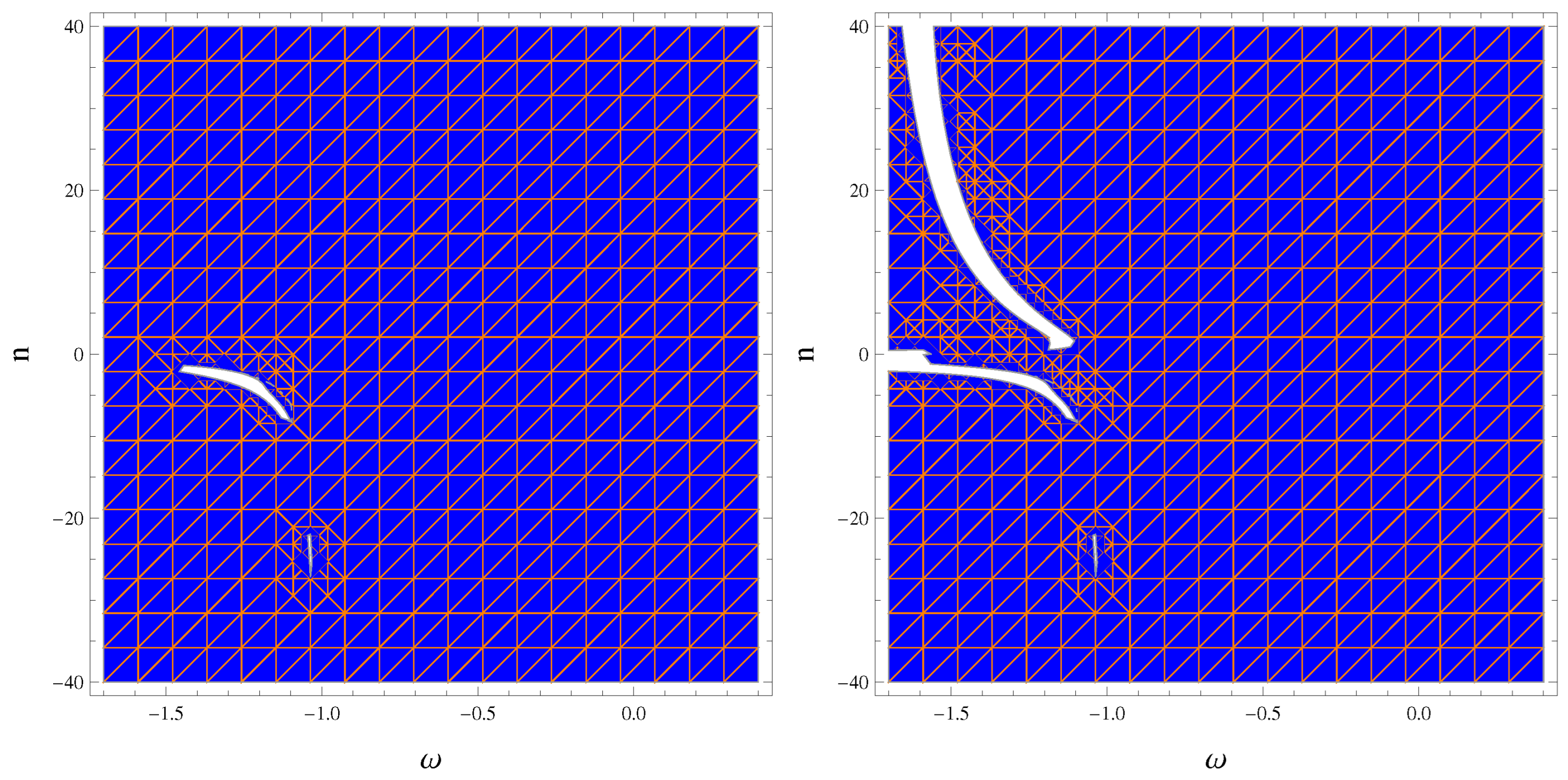
Figure 2.
Stable regions of the ESU for , (blue) and (orange), corresponding to (left) and (right).

Figure 3.
Stable regions of the ESU for , (blue) and (orange), corresponding to (left) and (right).

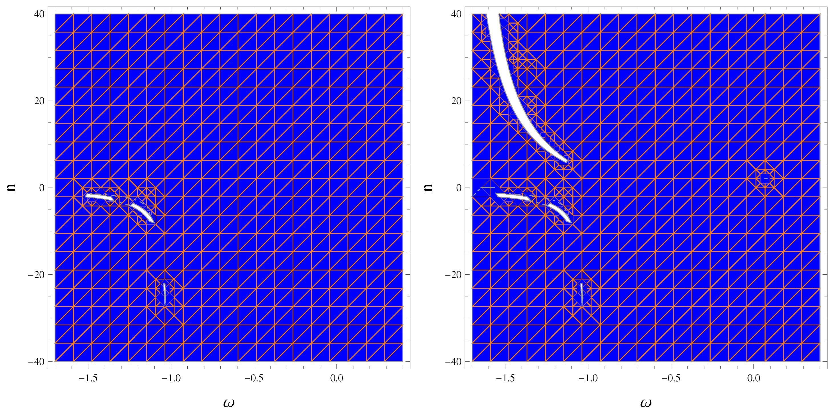
Figure 4.
Stable regions of the ESU for , (blue) and (orange), corresponding to (left) and (right).

Figure 5.
Stable regions of the ESU for , (blue) and (orange), corresponding to (left); (right).

Disclaimer/Publisher’s Note: The statements, opinions and data contained in all publications are solely those of the individual author(s) and contributor(s) and not of MDPI and/or the editor(s). MDPI and/or the editor(s) disclaim responsibility for any injury to people or property resulting from any ideas, methods, instructions or products referred to in the content. |
© 2023 by the authors. Licensee MDPI, Basel, Switzerland. This article is an open access article distributed under the terms and conditions of the Creative Commons Attribution (CC BY) license (https://creativecommons.org/licenses/by/4.0/).
Share and Cite
MDPI and ACS Style
Sharif, M.; Gul, M.Z. Stability Analysis of the Inhomogeneous Perturbed Einstein Universe in Energy–Momentum Squared Gravity. Universe 2023, 9, 145. https://doi.org/10.3390/universe9030145
AMA Style
Sharif M, Gul MZ. Stability Analysis of the Inhomogeneous Perturbed Einstein Universe in Energy–Momentum Squared Gravity. Universe. 2023; 9(3):145. https://doi.org/10.3390/universe9030145
Chicago/Turabian StyleSharif, Muhammad, and Muhammad Zeeshan Gul. 2023. "Stability Analysis of the Inhomogeneous Perturbed Einstein Universe in Energy–Momentum Squared Gravity" Universe 9, no. 3: 145. https://doi.org/10.3390/universe9030145
Note that from the first issue of 2016, this journal uses article numbers instead of page numbers. See further details here.