Introducing the Random Phase Approximation Theory

Abstract

Random Phase Approximation (RPA) is the theory most commonly used to describe the excitations of many-body systems. In this article, the secular equations of the theory are obtained by using three different approaches: the equation of motion method, the Green function perturbation theory and the time-dependent Hartree–Fock theory. Each approach emphasizes specific aspects of the theory overlooked by the other methods. Extensions of the RPA secular equations to treat the continuum part of the excitation spectrum and also the pairing between the particles composing the system are presented. Theoretical approaches which overcome the intrinsic approximations of RPA are outlined.

1. Introduction

The aim of the Random Phase Approximation (RPA) theory is the description of harmonic excitations of quantum many-body systems. This theory was formulated by David Bohm and David Pines in the early 1950s at the end of a set of articles dedicated to the description of collective oscillations of electron gas [1,2,3]. The approximation is well defined in the first of these articles [1], where it is used to eliminate the random movement of single electrons out of phase with respect to the oscillations of the external probe exciting the system. The theory is presented only in the third of these articles [3] and does not contain any random phase to be approximated. However, the authors used the term Random Phase Approximation to identify the theory and it is by this name that it is nowadays commonly known.

The applications of RPA in the 1950s and 1960s were focused on the description of infinite, homogeneous and translationally invariant systems, such as electron gas. A detailed historical overview of the works of these early years is given in Ref. [4]. Advances in the computing technologies allowed the application of RPA also to finite systems such as atoms and especially nuclei. During the 1970s and 1980s, RPA was the main theoretical tool used to investigate nuclear excitations of various types (see, for example, Refs. [5,6] for a review). More recently, RPA has been applied to atomic and molecular systems [7]. Nowadays, RPA calculations are rather standard and relatively simple to carry out, so that they are, improperly, classified as mean-field calculations.

RPA belongs to the category of effective theories. These theories use particle–particle interactions which do not have a strongly repulsive core at small inter-particle distances, a feature characterizing instead the microscopic interactions which are tailored to describe two-particle data. Hartree–Fock (HF) and Density Functional Theory (DFT) are also effective theories. They are conceived to describe the ground state of many-body systems, while RPA starts from the assumption that the ground state is known and considers the problem of describing the excitation modes.

The validity of RPA is restricted to situations where the excitation energies are relatively small as compared to the global binding energies of the system. This means that RPA is not suitable for describing situations where the system undergoes deep modifications of its structure, such as fission in nuclei or phase transitions in fluid.

In the energy regime adequate to be described by RPA, it is plausible to separate the role of the external probe, which excites the system, from its response. Each probe, photon, electron, neutrino, hadron, electric and magnetic field, sound wave, etc., is described by a specific set of operators depending on the type of interaction with the system. The response of the system depends only on the interactions between its fundamental components. For this reason, the many-body response is universal, independent of the specific probe that induces it. RPA evaluates this universal response.

Regarding the theoretical aspects of the theory, I like to quote what David Pines and Philippe Nozières write in Chapter 5.2 of their book on quantum liquids [8]:

“The development, frequent independent rediscovery and gradual appreciation of the Random Phase Approximation offers a useful lesson to theoretical physicist. First, it illustrates the splendid variety of ways that can be developed for saying the same thing. Second, it suggests the usefulness of learning different languages of theoretical physics and of attempting the reconciliation of seemingly different, but obviously related results."

Despite this clear statement, RPA is commonly presented in the context of specific theoretical frameworks in order to attack some well identified problem. In this article, I want to focus attention on the theory in itself and I present three different ways of obtaining the secular RPA equations. In my opinion, this allows a richer comprehension of the theory, since each method emphasizes aspects overlooked by the other ones. The present article is not a review of the recent advances in the use of RPA theory, but it aims to be a guide to understand it by pointing out its underlying assumptions, its merits and its faults and by indicating how to improve it.

The starting point of every many-body theory is the Independent Particle Model (IPM) and in Section 2, I recall some aspects of this model which are important for the RPA theory. RPA secular equations are derived in Section 3, Section 4 and Section 5 by using, respectively, the method of the equations of motion, the perturbation calculation of the two-body Green function and the harmonic approximation of the time-dependent evolution of the HF equations.

The following two sections are dedicated to specific aspects which can be considered by RPA. In Section 6, I present how to describe the fact that one particle can be emitted from the system, and in Section 7 how to treat pairing effects between the particles. Some issues related to the pragmatic application of RPA in actual calculations are presented in Section 8.

Approaches that extend the usual RPA formulations are outlined in Section 9, and the formulation of an RPA-like theory able to handle microscopic interactions is presented in Section 10.

Despite my good intentions, I used numerous acronyms and to facilitate the reading I list them in Abbreviations.

2. Independent Particle Models

The starting point of all the many-body theories is the Independent Particle Model (IPM). In this model, each particle moves independently of the presence of the other particles. This allows the definition of single-particle (s.p.) energies and wave functions identified by a set of quantum numbers. This is the basic language necessary to build any theory where the particles interact among them.

2.1. Mean-Field Model

A very general expression of the hamiltonian describing the many-body system is

$$\widehat{H}=\sum _{i=1}^A\left(-\frac{{\hslash }^2}{2m_i}{\nabla }_i^2+{\widehat{V}}_0\left(i\right)\right)+\frac{1}{2}\sum _{i,j=1}^A\widehat{V}(i,j)+\cdots ,$$

(1)

where A is the number of particles, each of them with mass $m_i$. In the expression (1), the term containing the Laplace operator ${\nabla }_i^2$ represents the kinetic energy, ${\widehat{V}}_0\left(i\right)$ is a generic potential acting on each particle and $\widehat{V}(i,j)$ is the interaction between two particles. The dots indicate the, eventual, presence of more complex terms of the interaction, such as three-body forces. Henceforth, we shall not consider these latter terms.

By adding to and subtracting from the expression (1) an average potential $\widehat{U}\left(i\right)$ acting on one particle at a time, we obtain:

$$\widehat{H}=\underset{{\widehat{H}}_0}{\underbrace{\sum _i^A\left(-\frac{{\hslash }^2}{2m_i}{\nabla }_i^2+{\widehat{V}}_0\left(i\right)+\widehat{U}\left(i\right)\right)}}+\underset{{\widehat{H}}_1}{\underbrace{\frac{1}{2}\sum _{i,j}^A\widehat{V}(i,j)-\sum _i^A\widehat{U}\left(i\right)}}.$$

(2)

The part indicated by ${\widehat{H}}_0$ is a sum of terms acting on one particle, the i-th particle, at a time. We can define each term of this sum as s.p. hamiltonian $\widehat{h}\left(i\right)$,

$${\widehat{H}}_0=\sum _i\widehat{h}\left(i\right)=\sum _i^A\left(-\frac{{\hslash }^2}{2m_i}{\nabla }_i^2+{\widehat{V}}_0\left(i\right)+\widehat{U}\left(i\right)\right).$$

(3)

The basic approximation of the Mean-Field (MF) model consists in neglecting, in the expression (2), the term ${\widehat{H}}_1$ called residual interaction. In this way, the many-body problem is transformed into a sum of many, independent, one-body problems, which can be solved one at a time. The MF model is an IPM since the particles described by ${\widehat{H}}_0$ do not interact among them.

The fact that the hamiltonian ${\widehat{H}}_0$ is a sum of independent terms implies that its eigenstates can be built as a product of the eigenstates of $\widehat{h}\left(i\right)$

$$\widehat{h}\left(i\right)|{\varphi }_i\rangle ={ϵ}_i|{\varphi }_i\rangle ,$$

(4)

therefore

$${\widehat{H}}_0|\Phi \rangle =\left(\sum _i\widehat{h}\left(i\right)\right)|\Phi \rangle =\mathcal{E}|\Phi \rangle ,$$

(5)

where

$$|\Phi \rangle =|{\varphi }_1\rangle |{\varphi }_2\rangle \cdots |{\varphi }_A\rangle .$$

(6)

For fermions, the antisymmetry of the global wave function under the exchange of two particles implies that the wave function $|\Phi \rangle$ has to be described as the sum of antisymmetrized products of one-particle wave functions. This solution is known in the literature as Slater determinant [9]

$$|\Phi \rangle =\frac{1}{\sqrt{A!}}det\left\{|{\varphi }_i\rangle \right\}.$$

(7)

Systems with global dimensions comparable to the average distances of two interacting particles are conveniently described by exploiting the spherical symmetry. We are talking about nuclei, atoms and small molecules. After choosing the center of the coordinate system, it is convenient to use polar spherical coordinates.

The single-particle wave function can be expressed as a product of a radial part, depending only on the distance $r\equiv |\mathbf{r}|$ from the coordinate center, with a term dependent on the angular coordinates $\theta$ and $\varphi$ and, eventually, the spin of the particle. The angular part has a well known analytic expression. For example, in cases of an MF potential containing a spin-orbit term the s.p. wave functions are conveniently expressed as:

$${\varphi }_{nljm}\left(\mathbf{r}\right)=R_{nlj}\left(r\right)\sum _{\mu \sigma }\langle l\mu \frac{1}{2}\sigma |jm\rangle Y_{l\mu }(\theta ,\varphi ){\chi }_{\sigma }=R_{nlj}\left(r\right){\mathcal{Y}}_{ljm}(\theta ,\varphi ),$$

(8)

where the spherical harmonics $Y_{l\mu }$ and the Pauli spinors ${\chi }_{\sigma }$ are connected by the Clebsch–Gordan coefficients and form the so-called spin spherical harmonics [10].

Systems with dimensions much larger than average distances between two interacting particles are conveniently described by exploiting the translational invariance. In condensed matter conglomerates, the translational symmetry dominates. A basic structure of the system is periodically repeated in three cartesian directions and it is not possible to find a central point.

The basic MF model for this type of system considers the potential $\widehat{U}$ to be constant. This fermionic system is commonly called Fermi gas. It is a toy model, homogeneous, with infinite volume, composed by an infinite number of fermions which do not interact with each other. Since the energy scale is arbitrary, it is possible to select $\widehat{U}=0$ without loosing generality. In this case, the one-body Schrödinger equation is

$$-\frac{{\hslash }^2}{2m_j}{\nabla }_j^2{\varphi }_j\left(\mathbf{r}\right)={ϵ}_j{\varphi }_j\left(\mathbf{r}\right).$$

(9)

By defining

$${ϵ}_j=\frac{{\hslash }^2{\mathbf{k}}_j^2}{2m_j},$$

(10)

the eigenfunction of Equation (9) can be written as

$${\varphi }_j\left(\mathbf{r}\right)=\frac{1}{\sqrt{\mathcal{V}}}{e}^{i{\mathbf{k}}_j·\mathbf{r}}{\chi }_{\sigma }{\chi }_{\tau },$$

(11)

where $\mathcal{V}$ is the volume of the system and $\chi$ are the Pauli spinors related to the spin of the fermion and, eventually, to its isospin. The third components of spin and isospin are indicated as $\sigma$ and $\tau$, respectively. The physical quantities of interest are those independent of $\mathcal{V}$ whose value, at the end of the calculations, is taken to be infinite.

The solution of the Fermi gas model provides a set of continuum single particle energies. Each energy is characterized by $k\equiv |\mathbf{k}|$, as indicated by Equation (10). In the ground state of the system, all the s.p. states with k smaller than a value $k_{\mathrm{F}}$, called Fermi momentum, are fully occupied and those with $k>k_{\mathrm{F}}$ are empty. Each state has a degeneracy of 2 in cases of electron gas and of 4 for nuclear matter where each nucleon is characterized also by the isospin third component.

2.2. Hartree–Fock Theory

The theoretical foundation of the MF model is provided by the Hartree–Fock (HF) theory, which is based on the application of the variational principle, one of the most used methods to solve the Schrödinger equation in an approximated manner. The basic idea is that the wave function which minimizes the energy, considered as functional of the many-body wave function, is the correct eigenfunction of the hamiltonian. This statement is correct when the search for the minimum is carried out by considering the full Hilbert space. In reality, the problem is simplified by assuming a specific expression of the wave function and the search for the minimum is carried out in the subspace spanned by all the wave functions which have the chosen expression. The energy value obtained in this manner is an upper bound of the correct energy eigenvalue of the hamiltonian. The formal properties of the variational principle are discussed in quantum mechanics textbooks.

For a fermion system, the HF equations are obtained by considering trial many-body wave functions which are expressed as a single Slater determinant. This implies the existence of an orthonormal basis of s.p. wave functions. The requirement that the s.p. wave functions are orthonormalized is a condition inserted in the variational equations in terms of Lagrange multipliers.

We continue this discussion by using Occupation Number Representation (ONR) formalism, which describes the operators acting on the Hilbert space in terms of creation ${\widehat{a}}_{\nu }^{+}$ and destruction ${\widehat{a}}_{\nu }$ operators. Concise presentations of this formalism are given in various textbooks, for example, in Appendix 2A of [11], in Appendix C of [12], in Appendix C of [13], in Chapter 4 of [14] and in Chapter 1 of [15].

In Appendix A we show that the hamiltonian of the many-body system, if only two-body interactions are considered, can be written as

$$\widehat{H}=\sum _{\nu }{ϵ}_{\nu }{\widehat{a}}_{\nu }^{+}{\widehat{a}}_{\nu }-\frac{1}{2}\sum _{ij}{\overline{V}}_{ijij}+\frac{1}{4}\sum _{\mu {\mu }^{\prime }\nu {\nu }^{\prime }}{\overline{V}}_{\nu \mu {\nu }^{\prime }{\mu }^{\prime }}\widehat{\mathbb{N}}\left[{\widehat{a}}_{\nu }^{+}{\widehat{a}}_{\mu }^{+}{\widehat{a}}_{{\mu }^{\prime }}{\widehat{a}}_{{\nu }^{\prime }}\right]={\widehat{H}}_0+{\widehat{V}}_{\mathrm{res}},$$

(12)

where ${\widehat{H}}_0$ is the sum of the first two terms, while ${\widehat{V}}_{\mathrm{res}}$ is the last term. We use the common convention of indicating with the latin letters $h,i,j,k,l$ s.p. states below the Fermi surface (hole states) and with the $m,n,p,q,r$ letters the s.p. states above the Fermi energies (particle states). Greek letters indicate indexes which have to be defined; therefore, in the above equation, their sums run on all the set of s.p. states. In Equation (12), ${ϵ}_{\nu }$ is the energy of the s.p. state characterized by the $\nu$ quantum numbers and $\overline{V}$ is the antisymmetrized matrix element of the interaction defined as

$${\overline{V}}_{\nu \mu {\nu }^{\prime }{\mu }^{\prime }}\equiv \langle \nu \mu |\widehat{V}|{\nu }^{\prime }{\mu }^{\prime }\rangle -\langle \nu \mu |\widehat{V}|{\mu }^{\prime }{\nu }^{\prime }\rangle .$$

(13)

With the symbol $\widehat{\mathbb{N}}$, we indicate the normal order operator which, by definition, arranges the set of creation and destruction operators in the brackets such that their expectation value on the ground state is zero. By considering this property of $\widehat{\mathbb{N}}$, the expectation value of the hamiltonian between two Slater determinants assumes the expression

$$\begin{array}{cc}& \langle {\Phi }_0|\widehat{H}|{\Phi }_0\rangle =\langle {\Phi }_0|{\widehat{H}}_0|{\Phi }_0\rangle +\langle {\Phi }_0|{\widehat{V}}_{\mathrm{res}}|{\Phi }_0\rangle \hfill \\ =& \sum _{\nu }{ϵ}_{\nu }\langle {\Phi }_0|{\widehat{a}}_{\nu }^{+}{\widehat{a}}_{\nu }|{\Phi }_0\rangle -\frac{1}{2}\sum _{ij}{\overline{V}}_{ijij}\langle {\Phi }_0|{\Phi }_0\rangle \hfill \\ +& \frac{1}{4}\sum _{\mu {\mu }^{\prime }\nu {\nu }^{\prime }}{\overline{V}}_{\nu \mu {\nu }^{\prime }{\mu }^{\prime }}\langle {\Phi }_0|\widehat{\mathbb{N}}\left[{\widehat{a}}_{\nu }^{+}{\widehat{a}}_{\mu }^{+}{\widehat{a}}_{{\mu }^{\prime }}{\widehat{a}}_{{\nu }^{\prime }}\right]|{\Phi }_0\rangle \hfill \\ =& \sum _i{ϵ}_i-\frac{1}{2}\sum _{ij}{\overline{V}}_{ijij}\equiv {\mathcal{E}}_0\left[{\Phi }_0\right],\hfill \end{array}$$

(14)

which clearly indicates that the contribution of the residual interaction is zero and the only part of the interaction which is considered is the one-body term ${\widehat{H}}_0$. This is a consequence of considering a single Slater determinant to describe the system ground state.

In Equation (14), we expressed the energy ${\mathcal{E}}_0$ as a functional of the Slater determinant ${\Phi }_0$. The search for the minimum of the energy functional is carried out in the Hilbert subspace spanned by Slater determinants. The quantities to be varied are the s.p. wave functions forming these determinants. These s.p. wave functions must be orthonormalized and this is an additional condition which has to be imposed in doing the variations. Therefore, the problem to be solved is the search for a constrained minimum and it is tackled by using the Lagrange multipliers technique.

The calculation is well known in the literature (see, for example, chapter XVIII-9 of [16] or Chapter 8.4 of [17]). The final result is a set of non-linear integro-differential equations providing the s.p. wave functions ${\varphi }_k$ and the values of the Lagrange multipliers ${ϵ}_k$. In coordinate space, these equations can be expressed as

$$\widehat{h}{\varphi }_k\left(\mathbf{r}\right)=-\frac{{\hslash }^2{\nabla }^2}{2m}{\varphi }_k\left(\mathbf{r}\right)+\underset{\mathrm{Hartree}}{\underbrace{\widehat{U}\left(\mathbf{r}\right){\varphi }_k\left(\mathbf{r}\right)}}-\underset{\mathrm{Fock}--\mathrm{Dirac}}{\underbrace{\int d^3{r}^{\prime }\widehat{W}(\mathbf{r},{\mathbf{r}}^{\prime }){\varphi }_k\left({\mathbf{r}}^{\prime }\right)}}={ϵ}_k{\varphi }_k\left(\mathbf{r}\right).$$

(15)

where the Hartree average potential is defined as

$$\widehat{U}\left(\mathbf{r}\right)\equiv \sum _j\int d^3{r}^{\prime }{\varphi }_j^{*}\left({\mathbf{r}}^{\prime }\right)\widehat{V}(\mathbf{r},{\mathbf{r}}^{\prime }){\varphi }_j\left({\mathbf{r}}^{\prime }\right),$$

(16)

and the non-local Fock–Dirac term is

$$\widehat{W}(\mathbf{r},{\mathbf{r}}^{\prime })\equiv \sum _j{\varphi }_j^{*}\left({\mathbf{r}}^{\prime }\right)\widehat{V}(\mathbf{r},{\mathbf{r}}^{\prime }){\varphi }_j\left(\mathbf{r}\right).$$

(17)

At this stage, the ${ϵ}_k$ are the values of the Lagrange multipliers. A theorem, called Koopmans [18], shows that these quantities are the differences between the energies of systems with $A+1$ and A particles; therefore, they are identified as s.p. energies.

By neglecting the Fock–Dirac term, we obtain a differential equation of MF type. The Fock–Dirac term, also called the exchange term, changes the bare mean-field equation by inserting the effect of the Pauli exclusion principle.

The differential Equation (15) is solved numerically by using an iterative procedure. One starts with a set of trial wave functions ${\varphi }_k^{\left(1\right)}$ built with MF methods. With these trial wave functions, the Hartree (16) and Fock–Dirac (17) terms are calculated and included in Equation (15) which is solved with standard numerical methods. In this way, a new set of s.p. wave functions ${\varphi }_k^{\left(2\right)}$ is obtained and it is used to calculate new $\widehat{U}$ and $\widehat{W}$ potentials. The process continues up to convergence.

As already pointed out in the introduction, the interactions used in the HF calculations are not the microscopic interactions built to reproduce the experimental data of the two-particle systems. These microscopic interactions contain a strongly repulsive core and, if inserted in the integrals of Equations (15) and (16), they would produce terms much larger than ${ϵ}_k$. This would attempt calculating a relatively small number by summing and subtracting relatively large numbers. HF calculations require interactions which have already tamed the strongly repulsive core (an early discussion of this problem can be found in Chapter 13 of [12]).

2.3. Density Functional Theory

The HF theory is widely utilized in nuclear and atomic physics, but there are two problems concerning its use. A first one is related to the formal development of the theory and it shows up mainly in the nuclear physics framework where the commonly used effective interactions have a phenomenological input containing also terms explicitly dependent on the density of the system. Without these terms, the HF calculations do not reproduce binding energies and densities of nuclei. The addition of these terms allows the construction of interactions able to produce high quality results all through the nuclide table. The physics simulated by these density dependent terms is still a matter of study. Formally, the variational principle used to derive the HF equation is not valid when the interaction depends explicitly on the density.

The second problem is of pragmatic type and it is related to the difficulty in evaluating the Fock–Dirac term of Equation (15) for complicated systems which do not show a well defined symmetry, for example, complex molecules.

The Density Functional Theory (DFT) solves both problems. This theory is based on a theorem of Hohenberg and Kohn [19], formulated in the 1960s.

Let us express the hamiltonian of a system of A fermions of mass m as:

$$\widehat{H}=\widehat{T}+{\widehat{U}}_{ext}+\widehat{V},$$

(18)

with

$$\widehat{T}=\sum _{i=1}^A-{\hslash }^2\frac{{▽}_i^2}{2m},{\widehat{U}}_{ext}=\sum _{i=1}^A{\widehat{u}}_{ext}\left(i\right),\widehat{V}=\frac{1}{2}\sum _{i,j=1}^A\widehat{v}(i,j),$$

(19)

The kinetic energy term, $\widehat{T}$ and the external potential ${\widehat{U}}_{ext}$, are one-body operators, while the interaction term $\widehat{V}$ is a two-body potential. The kinetic energy term plus $\widehat{V}$ are characteristic of the many-fermion system, while ${\widehat{U}}_{ext}$ depends on external situations and therefore, in principle, can be modified.

The Hohenberg–Kohn theorem states that there is a bijective correspondence between the external potential ${\widehat{U}}_{ext}$, the ground state $|{\mathrm{\Psi }}_0\rangle$ and the number density

$${\rho }_0\left(\mathbf{r}\right)=\langle {\mathrm{\Psi }}_0|\sum _{i=1}^A\delta (\mathbf{r}-{\mathbf{r}}_i)|{\mathrm{\Psi }}_0\rangle ,$$

(20)

of the system.

The theorem has the following implications.

(a)

Because of the bijective mapping

$${\widehat{U}}_{ext}⟺|{\mathrm{\Psi }}_0\rangle ⟺{\rho }_0.$$

(21)

we can consider the states $|{\mathrm{\Psi }}_0\rangle$ as functionals of the density ${\rho }_0$.

(b)

Because of (a), every observable is also a functional of ${\rho }_0$. Specifically, this is true for the energy of the system

$$E\left[{\rho }_0\right]=\langle \mathrm{\Psi }\left[{\rho }_0\right]|\widehat{H}|\mathrm{\Psi }\left[{\rho }_0\right]\rangle =F\left[{\rho }_0\right]+\int d^{3}r{\widehat{U}}_{ext}\left(\mathbf{r}\right){\rho }_0\left(\mathbf{r}\right),$$

(22)

where the universal part, the part independent of the external potential, is defined as

$$F\left[{\rho }_0\right]\equiv \langle \mathrm{\Psi }\left[{\rho }_0\right]|\left(\widehat{T}+\widehat{V}\right)|\mathrm{\Psi }\left[{\rho }_0\right]\rangle .$$

(23)

(c)

The variational principle implies that for each $\rho \ne {\rho }_0$ the following relation holds:

$$E_0\equiv E\left[{\rho }_0\right]<E\left[\rho \right].$$

(24)

The focus of the theory has moved from the many-body wave function $|{\mathrm{\Psi }}_0\rangle$ to the much simpler one-body density ${\rho }_0$. The idea of Kohn and Sham [20] is to reproduce the ground state density ${\rho }_0$ of a system of interacting fermions by using a fictitious system of non-interacting fermions. This is done by changing the external part of the hamiltonian. In this view, the density (20) is expressed as a sum of orthonormalized s.p. wave functions

$${\rho }_0\left(\mathbf{r}\right)=\sum _{i<{ϵ}_{\mathrm{F}}}{|{\varphi }_i^{\mathrm{KS}}\left(\mathbf{r}\right)|}^2,$$

(25)

where ${ϵ}_{\mathrm{F}}$ is the Fermi energy and KS indicates Kohn and Sham. The density (25) is generated by a one-body hamiltonian whose eigenstate is a Slater determinant $|{\Phi }^{\mathrm{KS}}\rangle$. The energy functional built in the Kohn and Sham approach is usually expressed as:

$$E\left[{\rho }_0\right]=T^{\mathrm{KS}}\left[{\rho }_0\right]+E_{\mathrm{H}}^{\mathrm{KS}}\left[{\rho }_0\right]+E_{\mathrm{ext}}^{\mathrm{KS}}\left[{\rho }_0\right]+E_{\mathrm{xc}}^{\mathrm{KS}}\left[{\rho }_0\right],$$

(26)

where there is a kinetic energy term,

$$T^{\mathrm{KS}}\left[{\rho }_0\right]=\langle {\Phi }^{\mathrm{KS}}|\widehat{T}|{\Phi }^{\mathrm{KS}}\rangle =\int d^{3}r\sum _i{\varphi }_i^{*\mathrm{KS}}\left(\mathbf{r}\right)\left(-\frac{{\hslash }^2{\nabla }^2}{2m}\right){\varphi }_i^{\mathrm{KS}}\left(\mathbf{r}\right),$$

(27)

a Hartree term,

$$E_{\mathrm{H}}^{\mathrm{KS}}\left[{\rho }_0\right]=\int d^3{r}_i\int d^3{r}_j{\rho }_0\left({\mathbf{r}}_i\right)\widehat{v}({\mathbf{r}}_i,{\mathbf{r}}_j){\rho }_0\left({\mathbf{r}}_j\right),$$

(28)

and an external mean-field term

$$E_{\mathrm{ext}}^{\mathrm{KS}}\left[{\rho }_0\right]=\int d^{3}r{\rho }_0\left({\mathbf{r}}_i\right){\widehat{U}}_{\mathrm{ext}}^{\mathrm{KS}}\left({\mathbf{r}}_i\right).$$

(29)

The additional term, $E_{\mathrm{xc}}^{\mathrm{KS}}$, is said to be of exchange and correlation.

The variational principle is applied to the energy functional (26) and the final result is, again, a set of non-linear integro-differential equations, which allows the evaluation of the Kohn and Sham s.p. wave functions

$$\left\{-\frac{{\hslash }^2{\nabla }^2}{2m}+\int d^3{r}_j\widehat{v}(\mathbf{r},{\mathbf{r}}_j){\rho }_0\left({\mathbf{r}}_j\right)+{\widehat{U}}_{\mathrm{ext}}^{\mathrm{KS}}\left(\mathbf{r}\right)+{\widehat{U}}_{\mathrm{xc}}^{\mathrm{KS}}\left(\mathbf{r}\right)\right\}{\varphi }_i^{\mathrm{KS}}\left(\mathbf{r}\right)={ϵ}_i{\varphi }_i^{\mathrm{KS}}\left(\mathbf{r}\right).$$

(30)

This set of equations is solved numerically with iterative techniques analogous to those used in the HF case. In Equation (30), only local terms appear, contrary to the HF equations which contain the non-local Fock–Dirac term. This makes the numerical solution of the KS equations much simpler than that of the HF equations and allows an application of the theory to systems difficult to treat with HF.

While the only input of the HF theory is the effective interaction $\widehat{V}$, in the DFT one has, in addition, to define the exchange and correlation term ${\widehat{U}}_{\mathrm{xc}}^{\mathrm{KS}}$. The strategy for choosing this term is an open problem of investigation in the field.

Formally speaking, the s.p. wave functions ${\varphi }^{\mathrm{KS}}$ and the Lagrange multipliers ${ϵ}_k$ of Equation (30) do not have a well defined physical interpretation. From the pragmatical point of view, the values of these latter quantities are very close to the s.p. energies of the HF theory defined by Koopmans’ theorem.

2.4. Excited States in the Independent Particle Model

The IPM is quite successful in describing the ground state properties of the fermion systems. This is also due to the fact that effective interactions are tailored to make this work. A good example of this is provided by the AMEDEE compilation of Hartree–Fock–Bogolioubov results concerning the ground states of nuclear isotope chains from $Z=6$ up to $Z=130$ [21]. Experimental values of binding energies and charge density radii are described with excellent accuracy by using a unique and universal effective nucleon–nucleon interaction. The situation changes immediately as soon as one tries to apply the same theoretical scheme to describe excited states.

The basic ansatz of the IPM is that a many fermion system can be described by a single Slater determinant $|\Phi \rangle$. The Slater determinant describing the ground state, $|{\Phi }_0\rangle$, has all the s.p. states below the Fermi energy (hole states) fully occupied, while those above it (particle states) are completely empty. In this picture, excited states are obtained by promoting particles from states below the Fermi surface to states above it. By using the ONR, this procedure can be formally described as

$$|{\Phi }_N\rangle ={\widehat{a}}_{p_1}^{+}\cdots {\widehat{a}}_{p_N}^{+}{\widehat{a}}_{h_1}\cdots {\widehat{a}}_{h_N}|{\Phi }_0\rangle ,$$

(31)

where the p’s indicate particle states and the h’s the hole states. The number N of creation or destruction operators is obviously smaller than A, the number of fermions. The state $|{\Phi }_N\rangle$ is a Slater determinant where N hole states have been changed with N particle states and it is the eigenstate of the IPM hamiltonian

$${\widehat{H}}_0|{\Phi }_N\rangle ={\mathcal{E}}_N|{\Phi }_N\rangle .$$

(32)

The excitation energy of this system is given by the difference between the s.p. energies of the particle states and that of the hole states

$${\omega }_N^{\mathrm{IPM}}\equiv {\mathcal{E}}_N-{\mathcal{E}}_0={ϵ}_{p_1}+{ϵ}_{p_2}+\cdots +{ϵ}_{p_N}-({ϵ}_{h_1}+{ϵ}_{h_2}+\cdots +{ϵ}_{h_N}).$$

(33)

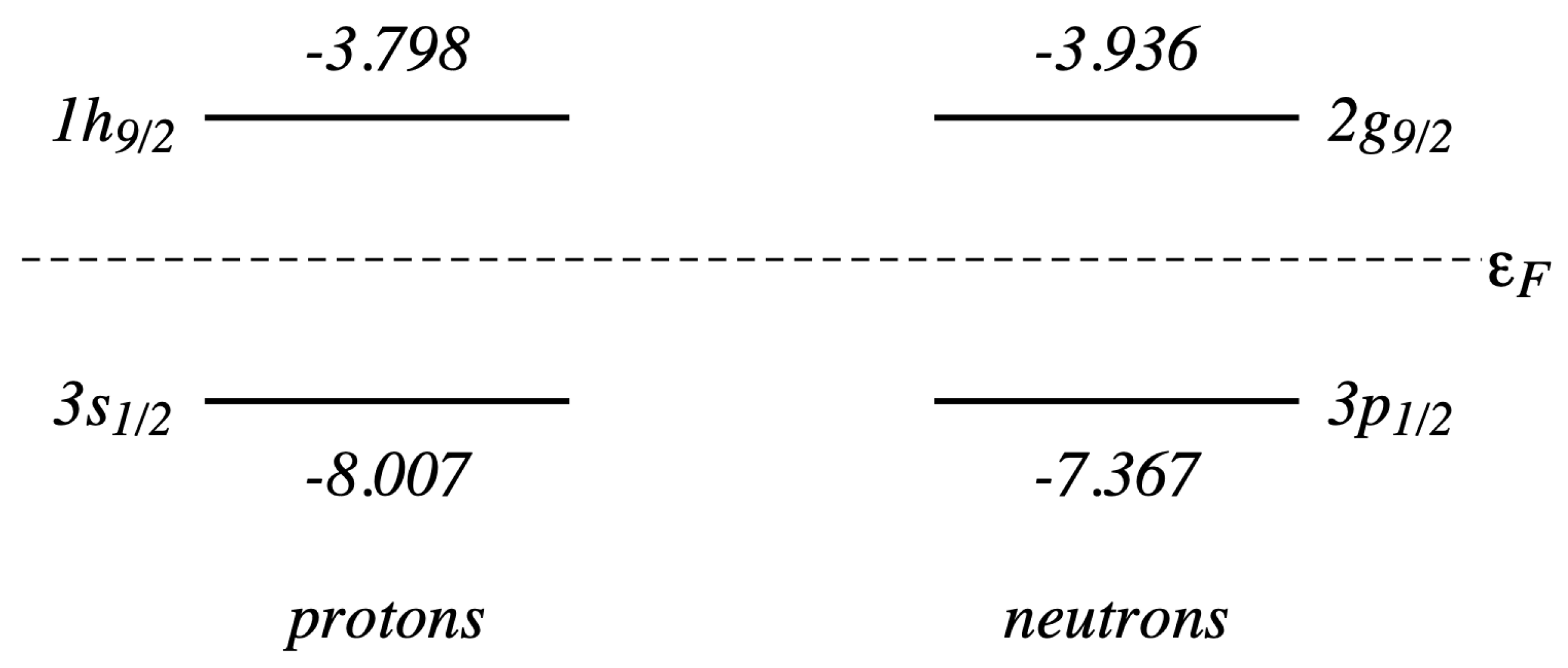
A good example of the failure of this approach in describing the excitations of a many-body systems is provided by the case of the ${}^{208}$Pb nucleus. We show in Figure 1 the scheme of the s.p. levels around the Fermi energy of this nucleus. The energies of these levels have been obtained by exploiting Koopmans’ theorem, i.e., by subtracting the experimental binding energies of the nuclei with one nucleon more or less, with respect to ${}^{208}$Pb. These nuclei are ${}^{207}$Tl, ${}^{209}$Bi and the two lead isotopes ${}^{207}$Pb and ${}^{209}$Pb. From the experimental values of the angular momenta of these odd–even nuclei, we identified the quantum numbers of the s.p. levels.

The first excited state in the IPM framework is that obtained by promoting the nucleon lying on the s.p. state just below the Fermi surface to the state just above it. In the present case, this one-particle one-hole ($1p-1h$) excitation for the protons will be produced by the transition from the $3s_{1/2}$ state to the $1h_{9/2}$ state. The excitation energy of this transition is 4.209 MeV, the parity is negative and the total angular momentum is 4 or 5. The analogous transition for the neutrons also implies a negative parity value and excitation energies of 3.431 MeV and also in this case the angular momentum values of the excited state can be 4 or 5. Measurements indicate that the first excited state of the ${}^{208}$Pb has an excitation energy of 2.614 MeV with angular momentum 3 and negative parity. Evidently, the IPM is unable to predict the presence of this state. The part of the hamiltonian disregarded by the IPM, the residual interaction, plays an important role. RPA considers the presence of the residual interaction in the description of the excitations of a many-body system.

3. RPA with the Equation of Motion Method

The first approach I present in order to obtain the RPA secular equations is the Equation of Motion (EOM) method inspired by the Heisenberg picture of quantum mechanics.

Let us define an operator, ${\widehat{Q}}_{\nu }^{+}$, whose action on the ground state of the system defines its excited states

$${\widehat{Q}}_{\nu }^{+}|{\mathrm{\Psi }}_0\rangle =|{\mathrm{\Psi }}_{\nu }\rangle ,$$

(34)

which satisfy the eigenvalue equation

$$\widehat{H}|{\mathrm{\Psi }}_{\nu }\rangle =E_{\nu }|{\mathrm{\Psi }}_{\nu }\rangle .$$

(35)

In the above equations, the index $\nu$ indicates all the quantum numbers characterizing the excited state. For example, in a finite fermion system, they are the excitation energy, the total angular momentum and the parity. The choice of ${\widehat{Q}}_{\nu }^{+}$ defines completely the problem to be solved, and also the ground state of the system through the equation

$${\widehat{Q}}_{\nu }|{\mathrm{\Psi }}_0\rangle =0.$$

(36)

It is worth remarking that the states $|{\mathrm{\Psi }}_{\nu }\rangle$ are not eigenstates of the full hamiltonian $\widehat{H}$ but, depending on the choice of ${\widehat{Q}}_{\nu }^{+}$, they are eigenstates of only a part of the hamiltonian. For example, if ${\widehat{Q}}_{\nu }^{+}={\widehat{a}}_p^{+}{\widehat{a}}_h$, ground and excited states are Slater determinants of the IPM described in Section 2.4. As has been already pointed out by discussing Equation (14), this choice does not consider the contribution of the residual interaction.

Let us calculate the commutator of the ${\widehat{Q}}_{\nu }^{+}$ operator with the hamiltonian

$$\begin{array}{ccc}\hfill \left[\widehat{H},{\widehat{Q}}_{\nu }^{+}\right]|{\mathrm{\Psi }}_0\rangle & =& \left(\widehat{H}{\widehat{Q}}_{\nu }^{+}-{\widehat{Q}}_{\nu }^{+}\widehat{H}\right)|{\mathrm{\Psi }}_0\rangle =\widehat{H}|{\mathrm{\Psi }}_{\nu }\rangle -{\widehat{Q}}_{\nu }^{+}{E}_0|{\mathrm{\Psi }}_0\rangle \hfill \\ & =& E_{\nu }|{\mathrm{\Psi }}_{\nu }\rangle -{\widehat{Q}}_{\nu }^{+}{E}_0|{\mathrm{\Psi }}_0\rangle =\left(E_{\nu }-E_0\right){\widehat{Q}}_{\nu }^{+}|{\mathrm{\Psi }}_0\rangle ,\hfill \end{array}$$

(37)

and for the operator ${\widehat{Q}}_{\nu }$, we obtain

$$\left[\widehat{H},{\widehat{Q}}_{\nu }\right]|{\mathrm{\Psi }}_0\rangle =\left(\widehat{H}{\widehat{Q}}_{\nu }-{\widehat{Q}}_{\nu }\widehat{H}\right)|{\mathrm{\Psi }}_0\rangle =\widehat{H}{\widehat{Q}}_{\nu }|{\mathrm{\Psi }}_0\rangle -E_0{\widehat{Q}}_{\nu }|{\mathrm{\Psi }}_0\rangle =0,$$

(38)

because of Equation (36).

We multiply Equation (37) by a generic operator $\widehat{\mathcal{O}}$ and by $\langle {\mathrm{\Psi }}_0|$ and we subtract the complex conjugate. For Equations (37) and (38), we obtain

$$\langle {\mathrm{\Psi }}_0|\left[\widehat{\mathcal{O}},[\widehat{H},{\widehat{Q}}_{\nu }^{+}]\right]|{\mathrm{\Psi }}_0\rangle =\left(E_{\nu }-E_0\right)\langle {\mathrm{\Psi }}_0|\widehat{\mathcal{O}}{\widehat{Q}}_{\nu }^{+}|{\mathrm{\Psi }}_0\rangle =\left(E_{\nu }-E_0\right)\langle {\mathrm{\Psi }}_0|\left[\widehat{\mathcal{O}},{\widehat{Q}}_{\nu }^{+}\right]|{\mathrm{\Psi }}_0\rangle .$$

(39)

since $\langle {\mathrm{\Psi }}_0|{\widehat{Q}}_{\nu }^{+}=0$.

This result is independent of the expression of the operator $\widehat{\mathcal{O}}$. In the construction of the various theories describing the system excited states, the $\widehat{\mathcal{O}}$ operator is substituted by the $\delta {\widehat{Q}}_{\nu }$ operator representing an infinitesimal variation of the excitation operator defined by Equation (34).

3.1. Tamm–Dankoff Approximation

A first choice of the ${\widehat{Q}}_{\nu }^{+}$ consists in considering the excited state as a linear combination of particle–hole excitations. This means that the excited state is not any more a single Slater determinant as in the IPM, but it is described by a sum of them. This choice of ${\widehat{Q}}_{\nu }^{+}$, leading to the so-called Tamm–Dankoff approximation (TDA), is

$${\widehat{Q}}_{\nu }^{+}\equiv \sum _{mi}{X}_{mi}^{\nu }{\widehat{a}}_m^{+}{\widehat{a}}_i,$$

(40)

where $X_{mi}^{\nu }$ is a real number and the usual convention of indicating the hole states with the letters $h,i,j,k,l$ and the particle states with $m,n,p,q,r$ has been adopted.

The definition (40) of the ${\widehat{Q}}_{\nu }^{+}$ operator implies that the ground state $|{\mathrm{\Psi }}_0\rangle$ satisfying Equations (37) and (38) is the IPM ground state $|{\Phi }_0\rangle$. In effect

$${\widehat{Q}}_{\nu }|{\Phi }_0\rangle =\sum _{mi}{X}_{mi}^{\nu }{\widehat{a}}_i^{+}{\widehat{a}}_m|{\Phi }_0\rangle =0,$$

(41)

since it is not possible to remove particles above the Fermi surface or to put particles below it.

An infinitesimal variation of the ${\widehat{Q}}_{\nu }$ operator can be expressed as

$$\delta {\widehat{Q}}_{\nu }=\sum _{mi}{\widehat{a}}_i^{+}{\widehat{a}}_m\delta X_{mi}^{*\nu },$$

(42)

since only the amplitudes $X_{mi}^{*\nu }$ can change. By substituting $\widehat{\mathcal{O}}$ with $\delta {\widehat{Q}}_{\nu }$ in Equation (39), we obtain

$$\begin{array}{cc}& \langle {\Phi }_0|\left[\sum _{mi}{\widehat{a}}_i^{+}{\widehat{a}}_m\delta X_{mi}^{*\nu },[\widehat{H},\sum _{nj}{X}_{nj}^{\nu }{\widehat{a}}_n^{+}{\widehat{a}}_j]\right]|{\Phi }_0\rangle \hfill \\ =& \left(E_{\nu }-E_0\right)\langle {\Phi }_0|[\sum _{mi}{\widehat{a}}_i^{+}{\widehat{a}}_m\delta X_{mi}^{*\nu },\sum _{nj}{X}_{nj}^{\nu }{\widehat{a}}_n^{+}{\widehat{a}}_j]|{\Phi }_0\rangle .\hfill \end{array}$$

(43)

Every variation $\delta X_{ph}^{*\nu }$ is independent of the other ones. For this reason, the above equation is a sum of terms independent of each other. The equation is satisfied if all the terms related to the same variation of $X_{ph}^{\nu }$ satisfy the relation. We can formally express this concept by considering a single term of the sum and by dividing it by $\delta X_{ph}^{*\nu }$ which is, by our choice, different from zero

$$\langle {\Phi }_0|\left[{\widehat{a}}_i^{+}{\widehat{a}}_m,[\widehat{H},\sum _{nj}{X}_{nj}^{\nu }{\widehat{a}}_n^{+}{\widehat{a}}_j]\right]|{\Phi }_0\rangle =\left(E_{\nu }-E_0\right)\sum _{nj}{X}_{nj}^{\nu }\langle {\Phi }_0|\left[a_i^{+}{a}_m,a_n^{+}{a}_j\right]|{\Phi }_0\rangle .$$

(44)

Let us calculate the right hand side of Equation (44):

$$\langle {\Phi }_0|\left[{\widehat{a}}_i^{+}{\widehat{a}}_m,{\widehat{a}}_n^{+}{\widehat{a}}_j\right]|{\Phi }_0\rangle =\langle {\Phi }_0|{\widehat{a}}_i^{+}{\widehat{a}}_m{\widehat{a}}_n^{+}{\widehat{a}}_j|{\Phi }_0\rangle -\langle {\Phi }_0|{\widehat{a}}_n^{+}{\widehat{a}}_j,{\widehat{a}}_i^{+}{\widehat{a}}_m|{\Phi }_0\rangle .$$

(45)

We apply Wick’s theorem (see, for example, Ref. [22]) to the first term

(46)

where the lines indicate the operators to be contracted.

The second term of Equation (45) is zero since ${\widehat{a}}_m|{\Phi }_0\rangle =0.$ By using this result in Equation (44), we obtain

$$\langle {\Phi }_0|\left[{\widehat{a}}_i^{+}{\widehat{a}}_m,[\widehat{H},\sum _{nj}{X}_{nj}^{\nu }{\widehat{a}}_n^{+}{\widehat{a}}_j]\right]|{\Phi }_0\rangle =\left(E_{\nu }-E_0\right)X_{mi}^{\nu }.$$

(47)

The evaluation of the double commutator of the left hand side of Equation (47) is explicitly presented in Appendix B. We insert the results of Equations (A14) and (A19) into Equation (47) and we consider the symmetry properties of the antisymmetrized matrix element of the interaction ${\overline{V}}_{\alpha ,\beta ,{\alpha }^{\prime },{\beta }^{\prime }}$, Equation (13). Finally, we obtain the TDA equations:

$$\sum _{nj}{X}_{nj}^{\nu }\left[({ϵ}_n-{ϵ}_j){\delta }_{mn}{\delta }_{ij}+{\overline{V}}_{mjin}\right]=(E_{\nu }-E_0)X_{mi}^{\nu }.$$

(48)

The expression (48) represents a homogenous system of linear equations whose unknowns are the $X_{mi}^{\nu }$. The number of unknowns, and therefore of solutions, is given by the number of particle–hole pairs which truncates the sum.

The normalization condition of the excited state induces a relation between the $X_{mi}^{\nu }$ amplitudes:

(49)

which defines without ambiguity the values of the $X_{ph}^{\nu }$ and suggests their probabilistic interpretation.

The TDA theory describes not only the energy spectrum of the system, but also for each excited state it provides the many-body wave function written in terms of single-particle states. This allows the calculation of the transition probability from the ground state to an excited state.

Let us assume that the action of the external field which excites the system is described by a one-body operator

$$\widehat{F}=\sum _{\mu {\mu }^{\prime }}\langle \mu |\widehat{f}|{\mu }^{\prime }\rangle {\widehat{a}}_{\mu }^{+}{\widehat{a}}_{{\mu }^{\prime }}\equiv \sum _{\mu {\mu }^{\prime }}{f}_{\mu {\mu }^{\prime }}{\widehat{a}}_{\mu }^{+}{\widehat{a}}_{{\mu }^{\prime }}.$$

(50)

The transition probability from the ground state to a TDA excited state is

$$\begin{array}{ccc}\hfill \langle {\mathrm{\Psi }}_{\nu }|\widehat{F}|{\mathrm{\Psi }}_0\rangle & =& \langle {\Phi }_0|{\widehat{Q}}_{\nu }\widehat{F}|{\Phi }_0\rangle \hfill \\ \hfill & =& \langle {\Phi }_0|\sum _{mi}{X}_{mi}^{*\nu }{\widehat{a}}_i^{+}{\widehat{a}}_m\sum _{\mu {\mu }^{\prime }}{f}_{\mu {\mu }^{\prime }}{\widehat{a}}_{\mu }^{+}{\widehat{a}}_{{\mu }^{\prime }}|{\Phi }_0\rangle \hfill \\ \hfill & =& \sum _{mi}{X}_{mi}^{*\nu }\sum _{\mu {\mu }^{\prime }}{f}_{\mu {\mu }^{\prime }}\langle {\Phi }_0|{\widehat{a}}_i^{+}{\widehat{a}}_m{\widehat{a}}_{\mu }^{+}{\widehat{a}}_{{\mu }^{\prime }}|{\Phi }_0\rangle \hfill \\ & =& \sum _{mi}{X}_{mi}^{*\nu }\sum _{\mu {\mu }^{\prime }}{f}_{\mu {\mu }^{\prime }}{\delta }_{i{\mu }^{\prime }}{\delta }_{m\mu }=\sum _{mi}{X}_{mi}^{*\nu }{f}_{mi}.\hfill \end{array}$$

(51)

where we used Wick’s theorem as in Equation (46). The many-body transition probabilities are described in terms of single-particle transition probabilities.

3.2. Random Phase Approximation

3.2.1. Limits of the TDA

The comparison between the TDA results and the experimental data is not satisfactory, especially in nuclear physics. For this reason, since the second half of the 1960s, the assumptions related to the TDA theory have been carefully analyzed. These assumptions are related to the choice of the expression (42) of the ${\widehat{Q}}_{\nu }$ operator. From these studies, it appeared clear that this choice is inconsistent with the equations of motion (39).

This inconsistency can be seen in the following manner. The equation of motions (39) were obtained without making any assumption on the operator $\widehat{\mathcal{O}}$. For the operator $\widehat{\mathcal{O}}={\widehat{a}}_m^{+}{\widehat{a}}_i$, the equations of motion are:

$$\langle {\mathrm{\Psi }}_0|\left[{\widehat{a}}_m^{+}{\widehat{a}}_i,[\widehat{H},{\widehat{Q}}_{\nu }^{+}]\right]|{\mathrm{\Psi }}_0\rangle =\left(E_{\nu }-E_0\right)\langle {\mathrm{\Psi }}_0|{\widehat{a}}_m^{+}{\widehat{a}}_i{\widehat{Q}}_{\nu }^{+}|{\mathrm{\Psi }}_0\rangle =\left(E_{\nu }-E_0\right)\langle {\mathrm{\Psi }}_0|\left[{\widehat{a}}_m^{+}{\widehat{a}}_i,{\widehat{Q}}_{\nu }^{+}\right]|{\mathrm{\Psi }}_0\rangle .$$

(52)

By inserting the expression of the TDA operator (42) in the right hand side of the above equation, we obtain

$$\sum _{nj}{X}_{nj}^{\nu }\langle {\Phi }_0|\left[{\widehat{a}}_m^{+}{\widehat{a}}_i,{\widehat{a}}_n^{+}{\widehat{a}}_j\right]|{\Phi }_0\rangle =\sum _{nj}{X}_{nj}^{\nu }\left\{\langle {\Phi }_0|{\widehat{a}}_m^{+}{\widehat{a}}_i{\widehat{a}}_n^{+}{\widehat{a}}_j|{\Phi }_0\rangle -\langle {\Phi }_0|{\widehat{a}}_n^{+}{\widehat{a}}_j{\widehat{a}}_m^{+}{\widehat{a}}_i|{\Phi }_0\rangle \right\}=0.$$

(53)

This result requires that also the left hand side of Equation (52) be zero. The one-body term of the hamiltonian has a double commutator equal to zero

$$\sum _{\alpha \beta }{h}_{\alpha ,\beta }\langle {\Phi }_0|\left[{\widehat{a}}_m^{+}{\widehat{a}}_i,({\widehat{a}}_{\alpha }^{+}{\widehat{a}}_j{\delta }_{n\beta }-{\widehat{a}}_n^{+}{\widehat{a}}_{\beta }{\delta }_{j\alpha })\right]|{\Phi }_0\rangle =0,$$

but the double commutator of the interaction term is not equal to zero.

$$\sum _{\alpha ,\beta ,{\alpha }^{\prime },{\beta }^{\prime }}{\overline{V}}_{\alpha ,\beta ,{\alpha }^{\prime },{\beta }^{\prime }}\langle {\Phi }_0|\left[{\widehat{a}}_m^{+}{\widehat{a}}_i,\left[\widehat{\mathbb{N}}\left[{\widehat{a}}_{\alpha }^{+}{\widehat{a}}_{\beta }^{+}{\widehat{a}}_{{\beta }^{\prime }}{\widehat{a}}_{{\alpha }^{\prime }}\right],{\widehat{a}}_n^{+}{\widehat{a}}_j\right]\right]|{\Phi }_0\rangle \ne 0.$$

3.2.2. RPA Equations

The most straightforward way of extending the TDA is to consider the RPA excitation operator (42) defined as

$${\widehat{Q}}_{\nu }^{+}\equiv \sum _{ph}{X}_{ph}^{\nu }{\widehat{a}}_p^{+}{\widehat{a}}_h-\sum _{ph}{Y}_{ph}^{\nu }{\widehat{a}}_h^{+}{\widehat{a}}_p,$$

(54)

where both $X_{ph}^{\nu }$ and $Y_{ph}^{\nu }$ are numbers.

RPA ground state is defined by the equation ${\widehat{Q}}_{\nu }|{\nu }_0\rangle =0$. Evidently $|{\nu }_0\rangle$ is not an IPM ground state, i.e., a single Slater determinant. In this last case, we would have

$${\widehat{Q}}_{\nu }|{\Phi }_0\rangle =\sum _{ph}{X}_{ph}^{*\nu }{\widehat{a}}_h^{+}{\widehat{a}}_p|{\Phi }_0\rangle -\sum _{ph}{Y}_{ph}^{*\nu }{\widehat{a}}_p^{+}{\widehat{a}}_h|{\Phi }_0\rangle \ne 0.$$

The first term is certainly zero, while the second one is not zero. RPA ground state $|{\nu }_0\rangle$ is more complex than the IPM ground state and it contains effects beyond it. These effects, called generically correlations, are here described in terms of hole–particle excitations, as we shall discuss in Section 3.2.6.

From the definition (54) of RPA amplitudes, we obtain $\delta {\widehat{Q}}_{\nu }$ and by inserting it as $\widehat{\mathcal{O}}=\delta {\widehat{Q}}_{\nu }$ in the equations of motion (39) we obtain

$$\begin{array}{ccc}\hfill & & \sum _{mi}\delta X_{mi}^{\nu }\langle {\nu }_0|\left[{\widehat{a}}_i^{+}{\widehat{a}}_m,\left[\widehat{H},{\widehat{Q}}_{\nu }^{+}\right]\right]|{\nu }_0\rangle -\sum _{mi}\delta Y_{mi}^{\nu }\langle {\nu }_0|\left[{\widehat{a}}_m^{+}{\widehat{a}}_i,\left[\widehat{H},{\widehat{Q}}_{\nu }^{+}\right]\right]|{\nu }_0\rangle \hfill \\ & =& (E_{\nu }-E_0)\left\{\sum _{mi}\delta X_{mi}^{\nu }\langle {\nu }_0|\left[{\widehat{a}}_i^{+}{\widehat{a}}_m,{\widehat{Q}}_{\nu }^{+}\right]|{\nu }_0\rangle -\sum _{mi}\delta Y_{mi}^{\nu }\langle {\nu }_0|\left[{\widehat{a}}_m^{+}{\widehat{a}}_i,{\widehat{Q}}_{\nu }^{+}\right]|{\nu }_0\rangle \right\}.\hfill \end{array}$$

(55)

As in the TDA case, the above equation represents a sum of independent terms since each variation is independent of the other ones. By making equal the terms related to the same variation, we obtain the following relations

$$\begin{array}{ccc}\hfill \langle {\nu }_0|\left[{\widehat{a}}_i^{+}{\widehat{a}}_m,\left[\widehat{H},{\widehat{Q}}_{\nu }^{+}\right]\right]|{\nu }_0\rangle & =& (E_{\nu }-E_0)\langle {\nu }_0|\left[{\widehat{a}}_i^{+}{\widehat{a}}_m,{\widehat{Q}}_{\nu }^{+}\right]|{\nu }_0\rangle \hfill \end{array}$$

(56)

$$\begin{array}{ccc}\hfill \langle {\nu }_0|\left[{\widehat{a}}_m^{+}{\widehat{a}}_i,\left[\widehat{H},{\widehat{Q}}_{\nu }^{+}\right]\right]|{\nu }_0\rangle & =& (E_{\nu }-E_0)\langle {\nu }_0|\left[{\widehat{a}}_m^{+}{\widehat{a}}_i,{\widehat{Q}}_{\nu }^{+}\right]|{\nu }_0\rangle .\hfill \end{array}$$

(57)

Let us consider the left hand side of Equation (56)

$$\begin{array}{ccc}\hfill & & \langle {\nu }_0|\left[{\widehat{a}}_i^{+}{\widehat{a}}_m,\left[\widehat{H},{\widehat{Q}}_{\nu }^{+}\right]\right]|{\nu }_0\rangle \hfill \\ \hfill & =& \sum _{nj}{X}_{nj}^{\nu }\langle {\nu }_0|\left[{\widehat{a}}_i^{+}{\widehat{a}}_m,\left[\widehat{H},{\widehat{a}}_n^{+}{\widehat{a}}_j\right]\right]|{\nu }_0\rangle -\sum _{nj}{Y}_{nj}^{\nu }\langle {\nu }_0|\left[{\widehat{a}}_i^{+}{\widehat{a}}_m,\left[\widehat{H},{\widehat{a}}_j^{+}{\widehat{a}}_n\right]\right]|{\nu }_0\rangle \hfill \\ & \equiv & \sum _{nj}{X}_{nj}^{\nu }{A}_{minj}+\sum _{nj}{Y}_{nj}^{\nu }{B}_{minj}.\hfill \end{array}$$

(58)

These equations define the elements of the A and B matrices.

We calculate the right hand side of Equation (56) by using an approximation known in the literature as Quasi-Boson-Approximation (QBA) consisting in assuming that the expectation value of a commutator between RPA ground states has the same value of the commutator between IPM states $|{\Phi }_0\rangle$. In the specific case under study, we have that

$$\langle {\nu }_0|\left[{\widehat{a}}_i^{+}{\widehat{a}}_m,{\widehat{Q}}_{\nu }^{+}\right]|{\nu }_0\rangle \simeq \langle {\Phi }_0|\left[{\widehat{a}}_i^{+}{\widehat{a}}_m,{\widehat{Q}}_{\nu }^{+}\right]|{\Phi }_0\rangle .$$

(59)

It is worth remarking that the QBA can be applied only for expectation values of commutators. The idea is that pairs of creation and destruction operators follow the rule

$$[{\widehat{a}}_i^{+}{\widehat{a}}_m,{\widehat{a}}_n^{+}{\widehat{a}}_j]\simeq {\delta }_{mn}{\delta }_{ij},$$

which means that the operators ${\widehat{\mathcal{O}}}_{im}\equiv {\widehat{a}}_i^{+}{\widehat{a}}_m$ and ${\widehat{\mathcal{O}}}_{jn}^{+}\equiv a_n^{+}{a}_j$ behave as boson operators.

By using the QBA, we can write

$$\begin{array}{ccc}\hfill & & \langle {\nu }_0|\left[{\widehat{a}}_i^{+}{\widehat{a}}_m,{\widehat{Q}}_{\nu }^{+}\right]|{\nu }_0\rangle \hfill \\ \hfill & \simeq & \sum _{nj}{X}_{nj}^{\nu }\langle {\Phi }_0|[{\widehat{a}}_i^{+}{\widehat{a}}_m,{\widehat{a}}_n^{+}{\widehat{a}}_j]|{\Phi }_0\rangle -\sum _{nj}{Y}_{nj}^{\nu }\langle {\Phi }_0|[{\widehat{a}}_i^{+}{\widehat{a}}_m,{\widehat{a}}_j^{+}{\widehat{a}}_n]|{\Phi }_0\rangle \hfill \\ \hfill & =& \sum _{nj}{X}_{nj}^{\nu }\left\{\langle {\Phi }_0|{\widehat{a}}_i^{+}{\widehat{a}}_m{\widehat{a}}_n^{+}{\widehat{a}}_j|{\Phi }_0\rangle -\langle {\Phi }_0|{\widehat{a}}_n^{+}{\widehat{a}}_j{\widehat{a}}_i^{+}{\widehat{a}}_m|{\Phi }_0\rangle \right\}\hfill \\ \hfill & -& \sum _{nj}{Y}_{nj}^{\nu }\left\{\langle {\Phi }_0|{\widehat{a}}_i^{+}{\widehat{a}}_m{\widehat{a}}_j^{+}{\widehat{a}}_n|{\Phi }_0\rangle -\langle {\Phi }_0|{\widehat{a}}_j^{+}{\widehat{a}}_n{\widehat{a}}_i^{+}{\widehat{a}}_m|{\Phi }_0\rangle \right\}\hfill \\ & =& \sum _{nj}{X}_{nj}^{\nu }\langle {\Phi }_0|{\widehat{a}}_i^{+}{\widehat{a}}_m{\widehat{a}}_n^{+}{\widehat{a}}_j|{\Phi }_0\rangle =X_{mi}^{\nu }{\delta }_{mn}{\delta }_{ij},\hfill \end{array}$$

(60)

where we have taken into account that the terms multiplying $Y_{nj}^{\nu }$ do not conserve the particle number and, furthermore, that $a_m|{\Phi }_0\rangle =0$. Equation (56) becomes

$$\sum _{nj}{X}_{nj}^{\nu }{A}_{minj}+\sum _{nj}{Y}_{nj}^{\nu }{B}_{minj}=(E_{\nu }-E_0)X_{mi}^{\nu }.$$

(61)

For the calculation of the left hand side of Equation (57), we consider that:

$${[\widehat{H},{\widehat{a}}_n^{+}{\widehat{a}}_j]}^{+}={(\widehat{H}{\widehat{a}}_n^{+}{\widehat{a}}_j-{\widehat{a}}_n^{+}{\widehat{a}}_j\widehat{H})}^{+}={\widehat{a}}_j^{+}{\widehat{a}}_n\widehat{H}-\widehat{H}{\widehat{a}}_j^{+}{\widehat{a}}_n=-[\widehat{H},{\widehat{a}}_j^{+}{\widehat{a}}_n],$$

(62)

since $\widehat{H}={\widehat{H}}^{+}$ and then

$${\left[{\widehat{a}}_i^{+}{\widehat{a}}_m,[\widehat{H},{\widehat{a}}_j^{+}{\widehat{a}}_n]\right]}^{+}=-\left[{\widehat{a}}_m^{+}{\widehat{a}}_i,-[\widehat{H},{\widehat{a}}_n^{+}{\widehat{a}}_j]\right]=\left[{\widehat{a}}_m^{+}{\widehat{a}}_i,[\widehat{H},{\widehat{a}}_n^{+}{\widehat{a}}_j]\right].$$

(63)

The double commutator becomes

$$\begin{array}{ccc}\hfill & & \langle {\nu }_0|\left[a_m^{+}{a}_i,\left[\widehat{H},Q_{\nu }^{+}\right]\right]|{\nu }_0\rangle \hfill \\ \hfill & =& \sum X_{nj}^{\nu }\langle {\nu }_0|\left[a_m^{+}{a}_i,\left[\widehat{H},a_n^{+}{a}_j\right]\right]|{\nu }_0\rangle -\sum Y_{nj}^{\nu }\langle {\nu }_0|\left[a_m^{+}{a}_i,\left[\widehat{H},a_j^{+}{a}_n\right]\right]|{\nu }_0\rangle \hfill \\ \hfill & =& \sum X_{nj}^{\nu }\langle {\nu }_0|{\left[a_i^{+}{a}_m,\left[\widehat{H},a_j^{+}{a}_n\right]\right]}^{+}|{\nu }_0\rangle -\sum Y_{nj}^{\nu }\langle {\nu }_0|{\left[a_i^{+}{a}_m,\left[\widehat{H},a_n^{+}{a}_j\right]\right]}^{+}|{\nu }_0\rangle \hfill \\ & =& \sum _{nj}{X}_{nj}^{\nu }(-B_{minj}^{*})+\sum _{nj}{Y}_{nj}^{\nu }(-A_{minj}^{*}),\hfill \end{array}$$

(64)

where we considered the definitions of the matrix elements A and B in Equation (58).

For the calculation of the right hand side of Equation (57) by using the QBA, we have

$$\langle {\nu }_0|\left[{\widehat{a}}_m^{+}{\widehat{a}}_i,Q_{\nu }^{+}\right]|{\nu }_0\rangle \to \left(\mathrm{QBA}\right)\to -\sum _{nj}{Y}_{nj}^{\nu }\langle {\Phi }_0|\left[{\widehat{a}}_m^{+}{\widehat{a}}_i,{\widehat{a}}_j^{+}{\widehat{a}}_n\right]|{\Phi }_0\rangle =Y_{mi}^{\nu }{\delta }_{ij}{\delta }_{mn};$$

(65)

therefore, Equation (57) becomes

$$\sum _{nj}{X}_{nj}^{\nu }(-B_{minj}^{*})+\sum _{nj}{Y}_{nj}^{\nu }(-A_{minj}^{*})=(E_{\nu }-E_0)Y_{mi}^{\nu }.$$

(66)

Equations (61) and (66) represent a homogenous system of linear equations whose unknowns are RPA amplitudes $X_{ph}^{\nu }$ and $Y_{ph}^{\nu }$. Usually, this system is presented as

$$\left(\begin{array}{cc}A& B\\ & \\ B^{*}& A^{*}\end{array}\right)\left(\begin{array}{c}{X}^{\nu }\\ \\ Y^{\nu }\end{array}\right)=(E_{\nu }-E_0)\left(\begin{array}{cc}I& 0\\ & \\ 0& -I\end{array}\right)\left(\begin{array}{c}{X}^{\nu }\\ \\ Y^{\nu }\end{array}\right)=(E_{\nu }-E_0)\left(\begin{array}{c}{X}^{\nu }\\ \\ -Y^{\nu }\end{array}\right),$$

(67)

where A and B are square matrices whose dimensions are those of the number of the particle–hole pairs describing the excitation, and X and Y are vectors of the same dimensions.

The expressions of the matrix elements of A and B in terms of effective interaction between two interacting particles are obtained as in Appendix B and they are:

$$\begin{array}{lll}{A}_{minj}\hfill & \to \left(\mathrm{QBA}\right)\to & \langle {\Phi }_0|\left[{\widehat{a}}_i^{+}{\widehat{a}}_m,\left[\widehat{H},{\widehat{a}}_n^{+}{\widehat{a}}_j\right]\right]|{\Phi }_0\rangle =({ϵ}_m-{ϵ}_i){\delta }_{mn}{\delta }_{ij}+{\overline{V}}_{mjin},\hfill \end{array}$$

(68)

$$\begin{array}{lll}{B}_{minj}\hfill & \to \left(\mathrm{QBA}\right)\to & -\langle {\Phi }_0|\left[{\widehat{a}}_i^{+}{\widehat{a}}_m,\left[\widehat{H},{\widehat{a}}_j^{+}{\widehat{a}}_n\right]\right]|{\Phi }_0\rangle ={\overline{V}}_{mnij}.\hfill \end{array}$$

(69)

3.2.3. Properties of RPA Equations

We consider RPA equations in the form

$$\left(\begin{array}{cc}A& B\\ & \\ B^{*}& A^{*}\end{array}\right)\left(\begin{array}{c}{X}^{\nu }\\ \\ Y^{\nu }\end{array}\right)={\omega }_{\nu }\left(\begin{array}{c}{X}^{\nu }\\ \\ -Y^{\nu }\end{array}\right),$$

where ${\omega }_{\nu }=E_{\nu }-E_0$ is the excitation energy.

• If $B=0$, we obtain the TDA equations.
• We take the complex conjugate of the above equations and obtain

  $$\left(\begin{array}{cc}A& B\\ & \\ B^{*}& A^{*}\end{array}\right)\left(\begin{array}{c}{Y}^{*\nu }\\ \\ X^{*\nu }\end{array}\right)=-{\omega }_{\nu }\left(\begin{array}{c}{Y}^{*\nu }\\ \\ -X^{*\nu }\end{array}\right).$$

  (70)
  This indicates that RPA equations are satisfied by positive and negative eigenvalues with the same absolute value.
• Eigenvectors corresponding to different eigenvalues are orthogonal.

  $$\left(\begin{array}{cc}A& B\\ & \\ B^{*}& A^{*}\end{array}\right)\left(\begin{array}{c}{X}^{\nu }\\ \\ Y^{\nu }\end{array}\right)={\omega }_{\nu }\left(\begin{array}{c}{X}^{\nu }\\ \\ -Y^{\nu }\end{array}\right);\left(\begin{array}{cc}A& B\\ & \\ B^{*}& A^{*}\end{array}\right)\left(\begin{array}{c}{X}^{\mu }\\ \\ Y^{\mu }\end{array}\right)={\omega }_{\mu }\left(\begin{array}{c}{X}^{\mu }\\ \\ -Y^{\mu }\end{array}\right).$$
  Let us calculate the hermitian conjugate of the second equation

  $$({X^{\mu }}^{+},{Y^{\mu }}^{+})\left(\begin{array}{cc}A& B\\ & \\ B^{*}& A^{*}\end{array}\right)=({X^{\mu }}^{+},-Y^{\mu }){\omega }_{\mu }.$$
  We multiply the first equation by $({X^{\mu }}^{+},{Y^{\mu }}^{+})$ on the left hand side, and the second equation on the right hand side by

  $$\left(\begin{array}{c}{X}^{\nu }\\ \\ -Y^{\nu }\end{array}\right),$$

  and we obtain

  $$\begin{array}{ccc}\hfill ({X^{\mu }}^{+},{Y^{\mu }}^{+})\left(\begin{array}{cc}A& B\\ & \\ B^{*}& A^{*}\end{array}\right)\left(\begin{array}{c}{X}^{\nu }\\ \\ Y^{\nu }\end{array}\right)& =& {\omega }_{\nu }({X^{\mu }}^{+},{Y^{\mu }}^{+})\left(\begin{array}{c}{X}^{\nu }\\ \\ -Y^{\nu }\end{array}\right)\hfill \\ \hfill & & \\ \hfill ({X^{\mu }}^{+},{Y^{\mu }}^{+})\left(\begin{array}{cc}A& B\\ & \\ B^{*}& A^{*}\end{array}\right)\left(\begin{array}{c}{X}^{\nu }\\ \\ Y^{\nu }\end{array}\right)& =& {\omega }_{\mu }({X^{\mu }}^{+},-Y^{\mu })\left(\begin{array}{c}{X}^{\nu }\\ \\ Y^{\nu }\end{array}\right).\hfill \end{array}$$
  By subtracting the two equations, we have

  $$0=({\omega }_{\nu }-{\omega }_{\mu })({X^{\mu }}^{+}{X}^{\nu }-{Y^{\mu }}^{+}{Y}^{\nu }).$$
  Since we assumed ${\omega }_{\nu }\ne {\omega }_{\mu }$, we obtain

  $$({X^{\mu }}^{+}{X}^{\nu }-{Y^{\mu }}^{+}{Y}^{\nu })=0.$$
• The normalization between two excited states requires

  $$\begin{array}{ccc}\hfill {\delta }_{\nu {\nu }^{\prime }}& =& \langle \nu |{\nu }^{\prime }\rangle =\langle {\nu }_0|{\widehat{Q}}_{\nu }{\widehat{Q}}_{{\nu }^{\prime }}^{+}|{\nu }_0\rangle =\langle {\nu }_0|[{\widehat{Q}}_{\nu },{\widehat{Q}}_{{\nu }^{\prime }}^{+}]|{\nu }_0\rangle \to \mathrm{QBA}\to \langle {\Phi }_0|[{\widehat{Q}}_{\nu },{\widehat{Q}}_{{\nu }^{\prime }}^{+}]|{\Phi }_0\rangle \hfill \\ & =& \sum _{mi}\left(X_{mi}^{\nu }{X}_{mi}^{{\nu }^{\prime }}-Y_{mi}^{\nu }{Y}_{mi}^{{\nu }^{\prime }}\right),\hfill \end{array}$$

  (71)

  where we used the fact that ${\widehat{Q}}_{\nu }|{\nu }_0\rangle =0$ to express the operator as commutator in order to use the QBA.

3.2.4. Transition Probabilities in RPA

In analogy with the TDA case, we assume that the action of the external field exciting the system is described by a one-body operator expressed as in Equation (50). The transition probability between RPA ground state and excited state is described by

$$\langle \nu |\widehat{F}|{\nu }_0\rangle =\langle {\nu }_0|{\widehat{Q}}_{\nu }\widehat{F}|{\nu }_0\rangle =\langle {\nu }_0|[{\widehat{Q}}_{\nu },\widehat{F}]|{\nu }_0\rangle ,$$

(72)

where we used, again, the fact that ${\widehat{Q}}_{\nu }|{\nu }_0\rangle =0$. Since the equation is expressed in terms of commutator we can use the QBA

$$\begin{array}{ccc}\hfill & & \langle \nu |\widehat{F}|{\nu }_0\rangle \to \mathrm{QBA}\to \langle {\Phi }_0|[{\widehat{Q}}_{\nu },\widehat{F}]|{\Phi }_0\rangle \hfill \\ & =& \sum _{\mu {\mu }^{\prime }}{f}_{\mu {\mu }^{\prime }}\left\{\sum _{mi}{X}_{mi}^{\nu }\langle {\Phi }_0|[{\widehat{a}}_i^{+}{\widehat{a}}_m,{\widehat{a}}_{\mu }^{+}{\widehat{a}}_{{\mu }^{\prime }}]|{\Phi }_0\rangle -\sum _{mi}{Y}_{mi}^{\nu }\langle {\Phi }_0|[{\widehat{a}}_m^{+}{\widehat{a}}_i,{\widehat{a}}_{\mu }^{+}{\widehat{a}}_{{\mu }^{\prime }}]|{\Phi }_0\rangle \right\}.\hfill \end{array}$$

(73)

The two matrix elements are

$$\begin{array}{ccc}\hfill \langle {\Phi }_0|[{\widehat{a}}_i^{+}{\widehat{a}}_m,{\widehat{a}}_{\mu }^{+}{\widehat{a}}_{{\mu }^{\prime }}]|{\Phi }_0\rangle & =& \langle {\Phi }_0|{\widehat{a}}_i^{+}{\widehat{a}}_m{\widehat{a}}_{\mu }^{+}{\widehat{a}}_{{\mu }^{\prime }}|{\Phi }_0\rangle -\langle {\Phi }_0|{\widehat{a}}_{\mu }^{+}{\widehat{a}}_{{\mu }^{\prime }}{\widehat{a}}_i^{+}{\widehat{a}}_m|{\Phi }_0\rangle ={\delta }_{m\mu }{\delta }_{i{\mu }^{\prime }}-0,\hfill \\ \hfill \langle {\Phi }_0|[{\widehat{a}}_m^{+}{\widehat{a}}_i,{\widehat{a}}_{\mu }^{+}{\widehat{a}}_{{\mu }^{\prime }}]|{\Phi }_0\rangle & =& \langle {\Phi }_0|{\widehat{a}}_m^{+}{\widehat{a}}_i{\widehat{a}}_{\mu }^{+}{\widehat{a}}_{{\mu }^{\prime }}|{\Phi }_0\rangle -\langle {\Phi }_0|{\widehat{a}}_{\mu }^{+}{\widehat{a}}_{{\mu }^{\prime }}{\widehat{a}}_m^{+}{\widehat{a}}_i|{\Phi }_0\rangle =0-{\delta }_{m{\mu }^{\prime }}{\delta }_{i\mu };\hfill \end{array}$$

therefore,

$$\langle \nu |\widehat{F}|{\nu }_0\rangle \simeq \sum _{\mu {\mu }^{\prime }}{f}_{\mu {\mu }^{\prime }}\left(\sum _{mi}{X}_{mi}^{\nu }{\delta }_{m\mu }{\delta }_{i{\mu }^{\prime }}+\sum _{mi}{Y}_{mi}^{\nu }{\delta }_{m{\mu }^{\prime }}{\delta }_{i\mu }\right)=\sum _{mi}\left(X_{mi}^{\nu }{f}_{mi}+Y_{mi}^{\nu }{f}_{im}\right).$$

(74)

Also in RPA, the transition amplitude of a many-body system is expressed as a linear combination of single-particle transitions.

3.2.5. Sum Rules

We show in Appendix C that, in general, by indicating with $|{\mathrm{\Psi }}_{\nu }\rangle$ the eigenstates of the hamiltonian $\widehat{H}$

$$\widehat{H}|{\mathrm{\Psi }}_{\nu }\rangle =E_{\nu }|{\mathrm{\Psi }}_{\nu }\rangle ,$$

for an external operator $\widehat{F}$ inducing a transition of the system from the ground state to the excited state one has that:

$$2\sum _{\nu }(E_{\nu }-E_0){\left|\langle {\mathrm{\Psi }}_{\nu }|\widehat{F}|{\mathrm{\Psi }}_0\rangle \right|}^2=\langle {\mathrm{\Psi }}_0|\left[\widehat{F},\left[\widehat{H},\widehat{F}\right]\right]|{\mathrm{\Psi }}_0\rangle .$$

(75)

This expression puts a quantitative limit on the total value of the excitation strength of a many-body system. This value is determined only by the ground state properties and the knowledge of the excited states structure is not required. The validity of Equation (75) is related to the fact that the $|{\mathrm{\Psi }}_{\nu }\rangle$ are eigenstates of $\widehat{H}$. In actual calculations, states based on models or approximated solutions of the Schrödinger equations are used and Equation (75) is not properly satisfied.

On the other hand, for RPA theory, it has been shown [23] that the following relation holds

$$2\sum _{\nu }(E_{\nu }-E_0){\left|\langle \nu |\widehat{F}|{\nu }_0\rangle \right|}^2=\langle {\Phi }_0|\left[\widehat{F},\left[\widehat{H},\widehat{F}\right]\right]|{\Phi }_0\rangle .$$

(76)

The above expression, formally speaking, is not a true sum rule since in the left hand side there are RPA states, both ground and excited states, while in the right hand side there is an IPM ground state. These two types of states are not eigenstates of the same hamiltonian. When the residual interaction is neglected, one obtains mean-field excited states $|{\Phi }_{ph}\rangle$, i.e., single Slater determinants with a single particle–hole excitation. In this case, Equation (75) is verified since all these mean-field states are eigenstates of the unperturbed hamiltonian ${\widehat{H}}_0$

$$2\sum _{ph}({ϵ}_p-{ϵ}_h){\left|\langle {\Phi }_{ph}|\widehat{F}|{\Phi }_0\rangle \right|}^2=\langle {\Phi }_0|\left[\widehat{F},\left[{\widehat{H}}_0,\widehat{F}\right]\right]|{\Phi }_0\rangle ,$$

(77)

where the excitation energies of the full system are given by the difference between the single-particle energies of the particle–hole excitation.

Since in RPA the full hamiltonian $\widehat{H}={\widehat{H}}_0+{\widehat{V}}_{\mathrm{res}}$ is considered, by inserting this expression in Equation (76) we obtain

$$2\sum _{\nu }(E_{\nu }-E_0){\left|\langle \nu |\widehat{F}|{\nu }_0\rangle \right|}^2=\langle {\Phi }_0|\left[\widehat{F},\left[{\widehat{H}}_0,\widehat{F}\right]\right]|{\Phi }_0\rangle +\langle {\Phi }_0|\left[\widehat{F},\left[{\widehat{V}}_{\mathrm{res}},\widehat{F}\right]\right]|{\Phi }_0\rangle .$$

(78)

For operators $\widehat{F}$ which commute with ${\widehat{V}}_{\mathrm{res}}$, the IPM and RPA sum rules coincide.

3.2.6. RPA Ground State

We have already indicated that RPA ground state is not an IPM state but it contains effects beyond it, correlations, expressed in terms of hole–particle excitations. A more precise representation of the RPA ground state comes from a theorem demonstrated by D. J. Thouless [23] leading to an expression of the RPA ground state of the type [13]:

$$|{\nu }_0\rangle =\mathcal{N}{e}^{\widehat{S}}|{\Phi }_0\rangle ,$$

(79)

where $\mathcal{N}$ is a normalization constant and the operator $\widehat{S}$ is defined as

$$\widehat{S}\equiv \frac{1}{2}\sum _{\nu ,minj}{s}_{minj}^{\left(\nu \right)}{\widehat{a}}_m^{+}{\widehat{a}}_i{\widehat{a}}_j^{+}{\widehat{a}}_n.$$

(80)

The sum considers all the particle–hole, ${\widehat{a}}_m^{+}{\widehat{a}}_i$, and hole–particle, ${\widehat{a}}_j^{+}{\widehat{a}}_n$, pairs and the index $\nu$ runs on all the possible angular momentum and parity combinations allowed by the particle–hole and hole–particle quantum numbers. We indicated with $s_{minj}^{\left(\nu \right)}$ an amplitude weighting the contribution of each couple of $ph$.

Starting from the above expression, it is possible to calculate the $s_{minj}^{\left(\nu \right)}$ from the knowledge of RPA $X_{ph}^{\nu }$ and $Y_{ph}^{\nu }$ amplitudes [14]. By using these expressions, the expectation value of a one-body operator with respect to the RPA ground state can be expressed as [24,25]

$$\begin{array}{ccc}\hfill \langle {\nu }_0|\widehat{F}|{\nu }_0\rangle & =& \langle {\nu }_0|\sum _{\mu {\mu }^{\prime }}{f}_{\mu {\mu }^{\prime }}{\widehat{a}}_{\mu }^{+}{\widehat{a}}_{{\mu }^{\prime }}|{\nu }_0\rangle \hfill \\ & =& \sum _h{f}_{hh}\left[1-\frac{1}{2}\sum _{\nu }\sum _p{|Y_{ph}^{\nu }|}^2\right]+\sum _p{f}_{p,p}\left[\frac{1}{2}\sum _{\nu }\sum _h{|Y_{ph}^{\nu }|}^2\right].\hfill \end{array}$$

(81)

This clearly shows that the $Y_{ph}^{\nu }$ amplitudes modify the expectation value of the operator with respect to the IPM result. In TDA, the ground state is $|{\Phi }_0\rangle$ and the Y amplitudes are zero; therefore, the expectation value of $\widehat{F}$ is given by the sum of the s.p. expectation values of the states below the Fermi energy, as in the pure IPM. The TDA theory does not contain ground state correlations as indicated in Equation (41).

4. RPA with Green Function

4.1. Field Operators and Pictures

In this section, we use the field operators ${\widehat{\psi }}^{+}\left(\mathbf{r}\right)$, which creates a particle in the point $\mathbf{r}$. The hermitian conjugate operator $\widehat{\psi }\left(\mathbf{r}\right)$ destroys a particle positioned in $\mathbf{r}$. These two operators are related to the creation and destruction operators via the s.p. wave functions ${\varphi }_{\nu }\left(\mathbf{r}\right)$ generated by the solution of the IPM problem:

$$\widehat{\psi }\left(\mathbf{r}\right)=\sum _{\nu }{\widehat{a}}_{\nu }{\varphi }_{\nu }\left(\mathbf{r}\right);{\widehat{\psi }}^{+}\left(\mathbf{r}\right)=\sum _{\nu }{\widehat{a}}_{\nu }^{+}{\varphi }_{\nu }^{*}\left(\mathbf{r}\right).$$

(82)

These equations can be inverted to express the creation and destruction operators in terms of field operator

$${\widehat{a}}_{\nu }=\int d^{3}r{\varphi }_{\nu }^{*}\left(\mathbf{r}\right)\widehat{\psi }\left(\mathbf{r}\right);{\widehat{a}}_{\nu }^{+}=\int d^{3}r{\varphi }_{\nu }\left(\mathbf{r}\right){\widehat{\psi }}^{+}\left(\mathbf{r}\right).$$

(83)

where we exploited the orthonormality of the ${\varphi }_{\nu }$. By using the anti-commutation relations of the creation and destruction operators, see Equation (A3), we obtain analogous relations for the field operators:

$$\left\{{\widehat{\psi }}^{+}\left(\mathbf{r}\right),{\widehat{\psi }}^{+}\left({\mathbf{r}}^{\prime }\right)\right\}=0;\left\{\widehat{\psi }\left(\mathbf{r}\right),\widehat{\psi }\left({\mathbf{r}}^{\prime }\right)\right\}=0;\left\{{\widehat{\psi }}^{+}\left(\mathbf{r}\right),\widehat{\psi }\left({\mathbf{r}}^{\prime }\right)\right\}=\delta (\mathbf{r}-{\mathbf{r}}^{\prime }).$$

(84)

In the Heisenberg picture [16,22], the states are defined as

$$|{\mathrm{\Psi }}_{\mathrm{H}}\left(t\right)\rangle \equiv e^{i\frac{\widehat{H}t}{\hslash }}|{\mathrm{\Psi }}_{\mathrm{S}}\left(t\right)\rangle ,$$

(85)

with respect to those of the Schrödinger picture $|{\mathrm{\Psi }}_{\mathrm{S}}\left(t\right)\rangle$. In the above equations, $\widehat{H}$ is the full many-body hamiltonian. The states in the Heisenberg picture are time-independent and the time evolution of the system is described by the operators whose relation with the time-independent operators of the Schrödinger picture is:

$${\widehat{O}}_{\mathrm{H}}\equiv e^{i\frac{\widehat{H}t}{\hslash }}{\widehat{O}}_S{e}^{-i\frac{\widehat{H}t}{\hslash }},$$

(86)

satisfying the equation:

$$i\hslash \frac{\partial }{\partial t}{\widehat{O}}_{\mathrm{H}}\left(t\right)=[{\widehat{O}}_{\mathrm{H}}\left(t\right),\widehat{H}]$$

(87)

By separating the hamiltonian in the Schrödinger picture into two parts

$$\widehat{H}={\widehat{H}}_0+{\widehat{H}}_1,$$

(88)

it is possible to define an interaction picture whose states are defined as

$$|{\mathrm{\Psi }}_{\mathrm{I}}\left(t\right)\rangle \equiv e^{i\frac{{\widehat{H}}_{0}t}{\hslash }}|{\mathrm{\Psi }}_{\mathrm{S}}\left(t\right)\rangle ,$$

(89)

and the operators

$${\widehat{O}}_{\mathrm{I}}\left(t\right)=e^{i\frac{{\widehat{H}}_{0}t}{\hslash }}{\widehat{O}}_{\mathrm{S}}{e}^{-i\frac{{\widehat{H}}_{0}t}{\hslash }}.$$

(90)

In the interaction picture [22], both states and operators evolve with the time as indicated by the equations

$$i\hslash \frac{\partial }{\partial t}|{\mathrm{\Psi }}_{\mathrm{I}}\left(t\right)\rangle ={\widehat{H}}_{1,\mathrm{I}}\left(t\right)|{\mathrm{\Psi }}_{\mathrm{I}}\left(t\right)\rangle ,$$

(91)

and

$$i\hslash \frac{\partial }{\partial t}{\widehat{O}}_{\mathrm{I}}\left(t\right)=\left[{\widehat{O}}_{\mathrm{I}}\left(t\right),{\widehat{H}}_0\right].$$

(92)

The fermionic field operators in the Heisenberg and interaction picture are, respectively, defined as:

$${\widehat{\psi }}_{\mathrm{H}}(\mathbf{x},t)=e^{\frac{i}{\hslash }\widehat{H}t}\widehat{\psi }\left(\mathbf{x}\right)e^{-\frac{i}{\hslash }\widehat{H}t};{\widehat{\psi }}_{\mathrm{I}}(\mathbf{x},t)=e^{\frac{i}{\hslash }{\widehat{H}}_{0}t}\widehat{\psi }\left(\mathbf{x}\right)e^{-\frac{i}{\hslash }{\widehat{H}}_{0}t}$$

(93)

It can be shown that the anti-commutation relations (84) of the field operators, as well as those of the creation and destruction operators, see Equations (A3), are conserved in every representation [22].

4.2. Two-Body Green Function and RPA

The two-body Green function is defined as

$${(-i)}^2\mathrm{G}({\mathbf{x}}_1,t_1,{\mathbf{x}}_2,t_2,{\mathbf{x}}_3,t_3,{\mathbf{x}}_4,t_4)\equiv \frac{\langle {\mathrm{\Psi }}_0|\widehat{\mathbb{T}}\left[{\widehat{\psi }}_{\mathrm{H}}({\mathbf{x}}_1,t_1){\widehat{\psi }}_{\mathrm{H}}({\mathbf{x}}_2,t_2){\widehat{\psi }}_{\mathrm{H}}^{+}({\mathbf{x}}_3,t_3){\widehat{\psi }}_{\mathrm{H}}^{+}({\mathbf{x}}_4,t_4)\right]|{\mathrm{\Psi }}_0\rangle \rangle }{\langle {\mathrm{\Psi }}_0|{\mathrm{\Psi }}_0\rangle }.$$

(94)

In the above expression, $|{\mathrm{\Psi }}_0\rangle$ indicates the ground state of the system in Heisenberg representation and $\widehat{\mathbb{T}}$ is the time-ordering operator which arranges the field operators in decreasing time order. Because of the possible values that the times $t_i$ can assume, there are $4!=24$ cases, but, for the symmetry properties

$$\mathrm{G}(1,2,3,4)=-\mathrm{G}(2,1,3,4)=-\mathrm{G}(1,2,4,3)=\mathrm{G}(2,1,4,3),$$

(95)

only six of them are independent. Out of these six cases, only three have physically interesting properties and between these latter cases we select that where $t_1,t_3>t_2,t_4$ which implies

$${(-i)}^2\mathrm{G}({\mathbf{x}}_1,t_1,{\mathbf{x}}_2,t_2,{\mathbf{x}}_3,t_3,{\mathbf{x}}_4,t_4)=\frac{-\langle {\mathrm{\Psi }}_0|{\widehat{\psi }}_{\mathrm{H}}({\mathbf{x}}_1,t_1){\widehat{\psi }}_{\mathrm{H}}^{+}({\mathbf{x}}_3,t_3){\widehat{\psi }}_{\mathrm{H}}({\mathbf{x}}_2,t_2){\widehat{\psi }}_{\mathrm{H}}^{+}({\mathbf{x}}_4,t_4)|{\mathrm{\Psi }}_0\rangle }{\langle {\mathrm{\Psi }}_0|{\mathrm{\Psi }}_0\rangle },$$

(96)

and describes the time evolution of a $ph$ pair.

Since we work in a non-relativistic framework, the creation and also the destruction, of a particle–hole pair is instantaneous; therefore, we have that

$$t_1=t_3=t^{\prime }\mathrm{e}{t}_2=t_4=t.$$

(97)

For this case, we express the two-body Green function in terms of creation and destruction operators as

$$\begin{array}{ccc}\hfill & & \mathrm{G}({\mathbf{x}}_1,t^{\prime },{\mathbf{x}}_2,t,{\mathbf{x}}_3,t^{\prime },{\mathbf{x}}_4,t)\hfill \\ \hfill & =& \sum _{{\nu }_1{\nu }_2{\nu }_3{\nu }_4}\frac{{\varphi }_{{\nu }_1}\left({\mathbf{x}}_1\right){\varphi }_{{\nu }_3}^{*}\left({\mathbf{x}}_3\right){\varphi }_{{\nu }_2}\left({\mathbf{x}}_2\right){\varphi }_{{\nu }_4}^{*}\left({\mathbf{x}}_4\right)\langle {\mathrm{\Psi }}_0|\widehat{\mathbb{T}}\left[{\widehat{a}}_{{\nu }_1}\left(t^{\prime }\right){\widehat{a}}_{{\nu }_3}^{+}\left(t^{\prime }\right){\widehat{a}}_{{\nu }_2}\left(t\right){\widehat{a}}_{{\nu }_4}^{+}\left(t\right)\right]|{\mathrm{\Psi }}_0\rangle }{\langle {\mathrm{\Psi }}_0|{\mathrm{\Psi }}_0\rangle }\hfill \\ & =& \sum _{{\nu }_1{\nu }_2{\nu }_3{\nu }_4}{\varphi }_{{\nu }_1}\left({\mathbf{x}}_1\right){\varphi }_{{\nu }_2}\left({\mathbf{x}}_2\right){\varphi }_{{\nu }_3}^{*}\left({\mathbf{x}}_3\right){\varphi }_{{\nu }_4}^{*}\left({\mathbf{x}}_4\right)G({\nu }_1,t^{\prime },{\nu }_2,t,{\nu }_3,t^{\prime },{\nu }_4,t).\hfill \end{array}$$

(98)

where it is understood that all the creation and destruction operators are expressed in the Heisenberg picture. The previous equation defines a two-body Green function depending on the quantum numbers $\nu$ characterizing the single-particle states.

Since this Green function depends only on the time difference $\tau =t^{\prime }-t$, we find it convenient to define the energy dependent two-body Green function as

$$\tilde{G}({\nu }_1,{\nu }_2,{\nu }_3,{\nu }_4,E)={\int }_{-\infty }^{\infty }d\tau G({\nu }_1,{\nu }_2,{\nu }_3,{\nu }_4,\tau )e^{\frac{i}{\hslash }E\tau },$$

(99)

For the case $\tau >0$, by considering the expression of the creation and destruction operators in the Heisenberg picture, see Equation (86), and the fact that $|{\mathrm{\Psi }}_0\rangle$ is eigenstate of $\widehat{H}$ whose eigenvalue is $E_0$, we obtain the expression

$${\tilde{G}}_{\tau >0}({\nu }_1,{\nu }_2,{\nu }_3,{\nu }_4,E)=\frac{\langle {\mathrm{\Psi }}_0|{\widehat{a}}_{{\nu }_1}{\widehat{a}}_{{\nu }_3}^{+}{\int }_0^{\infty }d\tau e^{-\frac{i}{\hslash }(\widehat{H}-E_0-E)\tau }{\widehat{a}}_{{\nu }_2}{\widehat{a}}_{{\nu }_4}^{+}|{\mathrm{\Psi }}_0\rangle }{\langle {\mathrm{\Psi }}_0|{\mathrm{\Psi }}_0\rangle }.$$

(100)

We can express the value of the time integral as

$$\underset{\eta \to 0}{lim}{\int }_0^{\infty }d\tau e^{-\frac{i}{\hslash }(-\widehat{H}+E_0+E-i\eta )\tau }=\underset{\eta \to 0}{lim}\frac{-i\hslash }{E-\widehat{H}+E_0-i\eta };$$

(101)

therefore,

$${\tilde{G}}_{\tau >0}({\nu }_1,{\nu }_2,{\nu }_3,{\nu }_4,E)=\hslash \langle {\mathrm{\Psi }}_0|{\widehat{a}}_{{\nu }_1}{\widehat{a}}_{{\nu }_3}^{+}\frac{-i}{E-\widehat{H}+E_0+i\eta }{\widehat{a}}_{{\nu }_2}{\widehat{a}}_{{\nu }_4}^{+}|{\mathrm{\Psi }}_0\rangle \frac{1}{\langle {\mathrm{\Psi }}_0|{\mathrm{\Psi }}_0\rangle }.$$

(102)

With an analogous calculation for the $\tau <0$ case, we obtain

$$\begin{array}{ccc}\hfill \frac{i}{\hslash }\tilde{G}({\nu }_1,{\nu }_2,{\nu }_3,{\nu }_4,E)& =& \frac{i}{\hslash }({\tilde{G}}_{\tau >0}+{\tilde{G}}_{\tau <0})\hfill \\ \hfill & =& \langle {\mathrm{\Psi }}_0|{\widehat{a}}_{{\nu }_1}{\widehat{a}}_{{\nu }_3}^{+}\frac{1}{E-\widehat{H}+E_0-i\eta }{\widehat{a}}_{{\nu }_2}{\widehat{a}}_{{\nu }_4}^{+}|{\mathrm{\Psi }}_0\rangle \frac{1}{\langle {\mathrm{\Psi }}_0|{\mathrm{\Psi }}_0\rangle }\hfill \\ & -& \langle {\mathrm{\Psi }}_0|{\widehat{a}}_{{\nu }_2}{\widehat{a}}_{{\nu }_4}^{+}\frac{1}{E+\widehat{H}-E_0+i\eta }{\widehat{a}}_{{\nu }_1}{\widehat{a}}_{{\nu }_3}^{+}|{\mathrm{\Psi }}_0\rangle \frac{1}{\langle {\mathrm{\Psi }}_0|{\mathrm{\Psi }}_0\rangle }.\hfill \end{array}$$

(103)

By inserting the completeness of the eigenfunctions of $\widehat{H}$, ${\sum }_n|{\mathrm{\Psi }}_n\rangle \langle {\mathrm{\Psi }}_n|=1$ and considering $\widehat{H}|{\mathrm{\Psi }}_n\rangle =E_n|{\mathrm{\Psi }}_n\rangle$, we obtain the expression

$$\begin{array}{ccc}\hfill & & \frac{i}{\hslash }\tilde{G}({\nu }_1,{\nu }_2,{\nu }_3,{\nu }_4,E)=\frac{1}{\langle {\mathrm{\Psi }}_0|{\mathrm{\Psi }}_0\rangle }\hfill \\ & & \sum _n\left[\frac{\langle {\mathrm{\Psi }}_0|{\widehat{a}}_{{\nu }_1}{\widehat{a}}_{{\nu }_3}^{+}|{\mathrm{\Psi }}_n\rangle \langle {\mathrm{\Psi }}_n|{\widehat{a}}_{{\nu }_2}{\widehat{a}}_{{\nu }_4}^{+}|{\mathrm{\Psi }}_0\rangle }{E-(E_n-E_0)-i\eta }-\frac{\langle {\mathrm{\Psi }}_0|{\widehat{a}}_{{\nu }_2}{\widehat{a}}_{{\nu }_4}^{+}|{\mathrm{\Psi }}_n\rangle \langle {\mathrm{\Psi }}_n|{\widehat{a}}_{{\nu }_1}{\widehat{a}}_{{\nu }_3}^{+}|{\mathrm{\Psi }}_0\rangle }{E+(E_n-E_0)+i\eta }\right].\hfill \end{array}$$

(104)

In this expression, the states $|{\mathrm{\Psi }}_n\rangle$ have the same number of particles as the ground state. The energy values related to the poles, $E=E_n-E_0$, represent the excitation energies of the A particle system.

The unperturbed two-body Green function is obtained by substituting in Equation (104) the eigenstates $|\mathrm{\Psi }\rangle$ of the full hamiltonian with $|\Phi \rangle$, the eigenstates of the IPM hamiltonian ${\widehat{H}}_0$. In this case, the action of the creation and destruction operators is well defined and the energy eigenvalues are given by the s.p. energies of the $ph$ pair. Because of the properties of the creation and destruction operators we have that

$${\tilde{G}}^0(m,i,j,n,E)=\hslash \frac{{\delta }_{ij}{\delta }_{mn}}{{ϵ}_m-{ϵ}_i-E-i\eta },{\tilde{G}}^0(i,m,n,j,E)=\hslash \frac{{\delta }_{ij}{\delta }_{mn}}{{ϵ}_m-{ϵ}_i+E-i\eta },$$

(105)

and

$${\tilde{G}}^0(m,i,n,j,E)={\tilde{G}}^0(i,m,j,n,E)=0.$$

(106)

We show in Appendix D that the two-body Green function is strictly related to the response of the system to an external probe. By using $\widehat{F}$, the one-body operator of Equation (50) describing the action of the external probe, we can write the transition amplitude from the ground state to an excited state as

$$\begin{array}{ccc}\hfill S\left(E\right)& =& \sum _n|\langle {\mathrm{\Psi }}_0|\widehat{F}|{\mathrm{\Psi }}_n{\rangle |}^2\delta \left(E-(E_n-E_0)\right)\hfill \\ & =& \sum _{{\nu }_1{\nu }_2}\sum _{{\nu }_3{\nu }_4}{f}_{{\nu }_1{\nu }_2}{f}_{{\nu }_3{\nu }_4}^{*}\frac{\Im }{\pi }\left(i\hslash \tilde{G}({\nu }_1,{\nu }_3,{\nu }_2,{\nu }_4,E)\right),\hfill \end{array}$$

(107)

where $f_{{\nu }_1{\nu }_2}$ indicates the matrix element between s.p. wave functions.

The expression (107) of the transition amplitude separates the action of the external probe from the many-body response which is described by the two-body Green function. This latter quantity is related to the interaction between the particles composing the system and it is a universal function independent of the kind of probe perturbing the system. The knowledge of $S\left(E\right)$ allows a direct comparison with observable quantities such as scattering cross sections.

In the time-dependent perturbation theory, a theorem, called Gell–Man and Low, indicates that the eigenvector $|{\mathrm{\Psi }}_0\rangle$ of the full hamiltonian can be written as [22]:

$$\frac{\widehat{U}(0,-\infty )|{\Phi }_0\rangle }{\langle {\Phi }_0|\widehat{U}(0,-\infty )|{\Phi }_0\rangle }\equiv \frac{|{\mathrm{\Psi }}_0\rangle }{\langle {\Phi }_0|{\mathrm{\Psi }}_0\rangle },$$

(108)

where the time evolution operator $\widehat{U}$ can be expressed in powers of the interaction ${\widehat{H}}_1$ expressed in the interaction picture

$$\widehat{U}(t,t_0)=\sum _{n=0}^{\infty }{\left(\frac{-i}{\hslash }\right)}^n\frac{1}{n!}{\int }_{t_0}^{t}d{t}_1\dots {\int }_{t_0}^{t}d{t}_n\widehat{\mathbb{T}}\left[{\widehat{H}}_1\left(t_1\right)\dots {\widehat{H}}_1\left(t_n\right)\right].$$

(109)

In the above equation, we dropped the subindex $\mathrm{I}$ to simplify the writing.

We insert Equation (108) into the expression (94) of the two-body Green function and we obtain a perturbative expression of the full interacting Green function in powers of ${\widehat{H}}_1$ and of the unperturbed two-body Green function ${\mathrm{G}}^0$.

It is useful to consider a graphical representation of the Green function, as indicated in Figure 2. The full two-body Green function is indicated by two continuous thick lines. The upward arrows stand for the particle state and the downward for the hole. The continuous thin lines indicate the unperturbed Green function ${\mathrm{G}}^0$. In the figure, we consider only two-body interactions, i.e., ${\widehat{H}}_1=\widehat{\mathcal{U}}({\mathrm{x}}_1,{\mathrm{x}}_2)$ which is represented by a dashed line, with $\mathrm{x}$ indicating both space and time coordinates.

Figure 2 shows some of the terms we obtain by carrying out the perturbation expansion of the two-body Green function. The explicit expressions of the various terms are presented in Appendix E. We observe that there are diagrams which, by cutting particle and hole lines, can be separated into two diagrams already present in the expansion. This is the case, for example, of the diagram E of the figure which is composed by two diagrams of C type and by the diagram G which is given by the product of a diagram of C type and another one of F type. The contribution of these diagrams can be factorized in a term containing the four coordinates ${\mathrm{x}}_1\cdots {\mathrm{x}}_4$ of the full Green function times, another term which does not contain them. The sum of all the diagrams of this second type is identical to that of all the diagrams of the denominator; therefore, these two contributions simplify the matter. Finally, the calculation of $\mathrm{G}$ can be carried out by considering only the remaining diagrams of the numerators which are called irreducible.

Formally, this can be expressed with an equation similar to the Dyson’s equation for the one-body Green function [22]:

$$\begin{array}{ccc}\hfill & & \mathrm{G}({\mathrm{x}}_1,{\mathrm{x}}_2,{\mathrm{x}}_3,x_4)={\mathrm{G}}^0({\mathrm{x}}_1,{\mathrm{x}}_2,{\mathrm{x}}_3,{\mathrm{x}}_4)\hfill \\ & +& \int d^4{\mathrm{y}}_1{d}^4{\mathrm{y}}_2{d}^4{\mathrm{y}}_3{d}^4{\mathrm{y}}_4{\mathrm{G}}^0({\mathrm{x}}_1,{\mathrm{x}}_2,{\mathrm{y}}_1,{\mathrm{y}}_2)\widehat{\mathcal{K}}({\mathrm{y}}_1,{\mathrm{y}}_2,{\mathrm{y}}_3,{\mathrm{y}}_4)\mathrm{G}({\mathrm{y}}_3,{\mathrm{y}}_4,{\mathrm{x}}_3,{\mathrm{x}}_4).\hfill \end{array}$$

(110)

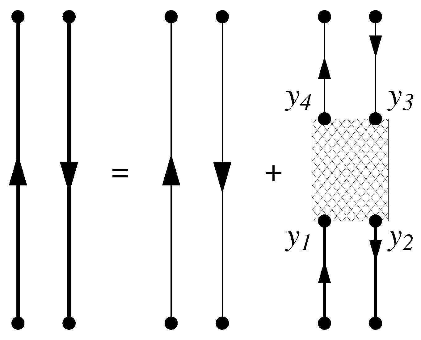
A graphical representation of Equation (110) is shown in Figure 3. The dashed area indicates the kernel $\widehat{\mathcal{K}}$ containing all the irreducible diagrams which can be inserted between the four y points.

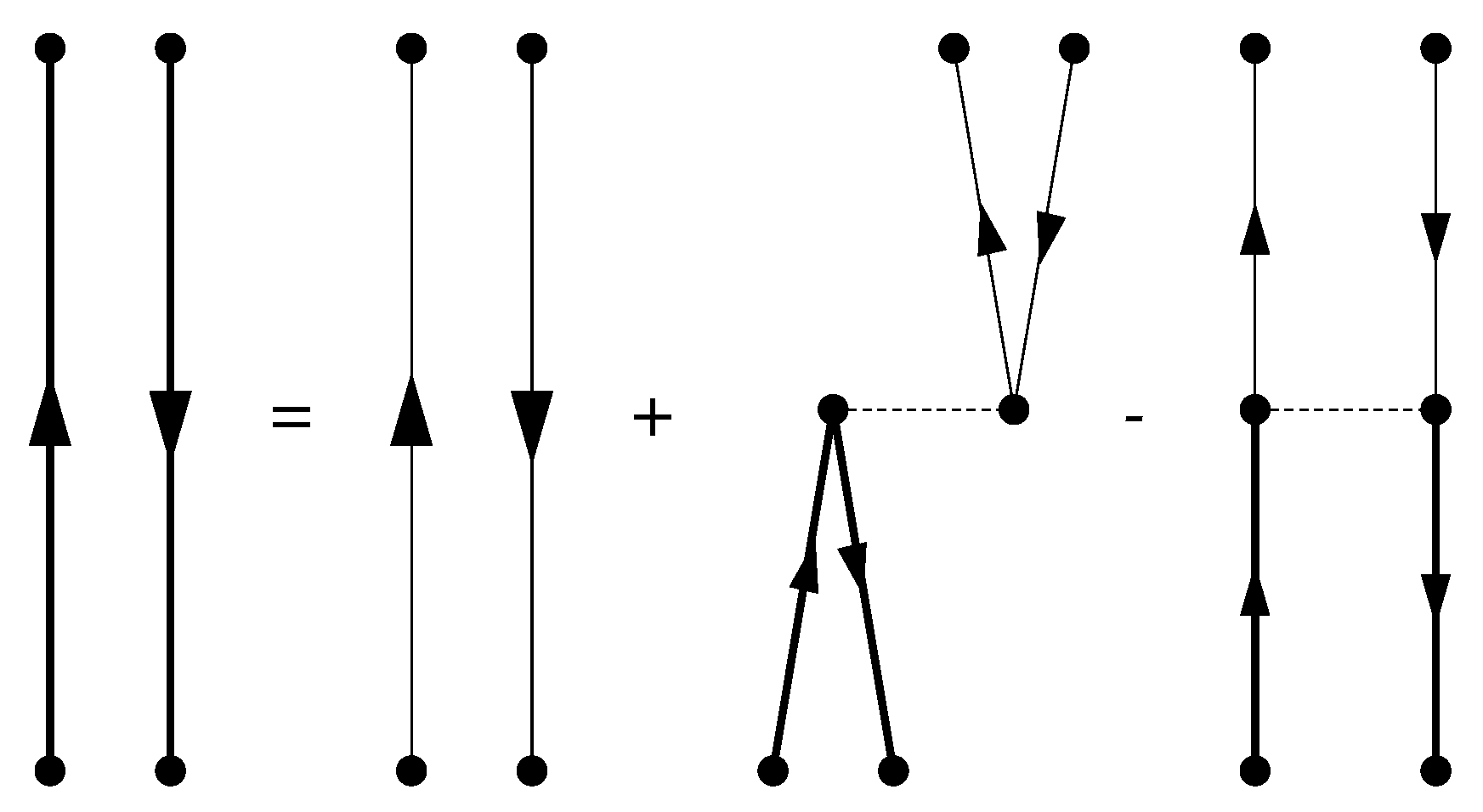
RPA consists in considering, in the previous equation, instead of the full kernel $\widehat{\mathcal{K}}$, a single interaction $\widehat{\mathcal{U}}$ depending only on two coordinates

$${\widehat{\mathcal{K}}}^{\mathrm{RPA}}({\mathrm{y}}_1,{\mathrm{y}}_2,{\mathrm{y}}_3,{\mathrm{y}}_4)=\widehat{\mathcal{U}}({\mathrm{y}}_1,{\mathrm{y}}_4)\left[\delta ({\mathrm{y}}_1-{\mathrm{y}}_2)\delta ({\mathrm{y}}_3-{\mathrm{y}}_4)-\delta ({\mathrm{y}}_1-{\mathrm{y}}_3)\delta ({\mathrm{y}}_2-{\mathrm{y}}_4)\right];$$

(111)

therefore,

$$\begin{array}{ccc}\hfill & & {\mathrm{G}}^{\mathrm{RPA}}({\mathrm{x}}_1,{\mathrm{x}}_2,{\mathrm{x}}_3,{\mathrm{x}}_4)={\mathrm{G}}^0({\mathrm{x}}_1,{\mathrm{x}}_2,{\mathrm{x}}_3,{\mathrm{x}}_4)\hfill \\ \hfill & +& \int d^4{\mathrm{y}}_1{d}^4{\mathrm{y}}_2{\mathrm{G}}^0({\mathrm{x}}_1,{\mathrm{x}}_2,{\mathrm{y}}_1,{\mathrm{y}}_1)\widehat{\mathcal{U}}({\mathrm{y}}_1,{\mathrm{y}}_2){\mathrm{G}}^{\mathrm{RPA}}({\mathrm{y}}_2,{\mathrm{y}}_2,{\mathrm{x}}_3,{\mathrm{x}}_4)\hfill \\ & -& \int d^4{y}_1{d}^4{y}_2{\mathrm{G}}^0({\mathrm{x}}_1,{\mathrm{x}}_2,{\mathrm{y}}_1,{\mathrm{y}}_2)\widehat{\mathcal{U}}({\mathrm{y}}_1,{\mathrm{y}}_2){\mathrm{G}}^{\mathrm{RPA}}({\mathrm{y}}_1,{\mathrm{y}}_2,{\mathrm{x}}_3,{\mathrm{x}}_4),\hfill \end{array}$$

(112)

where we separated the direct and the exchange terms. The graphical representation of the above equation is given in Figure 4.

In mixed representation, RPA equations are

$$\begin{array}{ccc}\hfill & & {\tilde{G}}^{\mathrm{RPA}}({\nu }_1,{\nu }_2,{\nu }_3,{\nu }_4,E)={\tilde{G}}^0({\nu }_1,{\nu }_2,{\nu }_3,{\nu }_4,E)\hfill \\ \hfill & +& \sum _{{\mu }_1,{\mu }_2,{\mu }_3,{\mu }_4}{\tilde{G}}^0({\nu }_1,{\nu }_2,{\mu }_1,{\mu }_2,E)\langle {\mu }_1{\mu }_3|\widehat{V}|{\mu }_2{\mu }_4\rangle {\tilde{G}}^{\mathrm{RPA}}({\mu }_3,{\mu }_4,{\nu }_3,{\nu }_4,E)\frac{1}{\hslash }\hfill \\ \hfill & -& \sum _{{\mu }_1,{\mu }_2,{\mu }_3,{\mu }_4}{\tilde{G}}^0({\nu }_1,{\nu }_2,{\mu }_1,{\mu }_2,E)\langle {\mu }_1{\mu }_2|\widehat{V}|{\mu }_4{\mu }_3\rangle {\tilde{G}}^{\mathrm{RPA}}({\mu }_3,{\mu }_4,{\nu }_3,{\nu }_4,E)\frac{1}{\hslash }\hfill \\ \hfill & =& \sum _{{\mu }_1,{\mu }_2,{\mu }_3,{\mu }_4}{\tilde{G}}^0({\nu }_1,{\nu }_2,{\mu }_1,{\mu }_2,E)\{{\delta }_{{\mu }_1,{\nu }_3}{\delta }_{{\mu }_2,{\nu }_4}\hfill \\ \hfill & +& \frac{1}{\hslash }\langle {\mu }_1{\mu }_3|\widehat{V}|{\mu }_2{\mu }_4\rangle {\tilde{G}}^{\mathrm{RPA}}({\mu }_3,{\mu }_4,{\nu }_3,{\nu }_4,E)\hfill \\ & -& \frac{1}{\hslash }\langle {\mu }_1{\mu }_2|\widehat{V}|{\mu }_4{\mu }_3\rangle {\tilde{G}}^{\mathrm{RPA}}({\mu }_3,{\mu }_4,{\nu }_3,{\nu }_4,E)\},\hfill \end{array}$$

(113)

where we used $\widehat{\mathcal{U}}=\widehat{V}/\hslash$.

As indicated by Equations (105) and (106), there are two possibilities of forming non-zero unperturbed Green functions. By adopting the usual convention of indicating with $i,j,k,l$ the hole states and with $m,n,p,q$ the particle states, we express RPA Equation (113) as:

$$\sum _{q,l}\left\{\left[A_{miql}-E{\delta }_{m,q}{\delta }_{i,l}\right]{\tilde{G}}^{\mathrm{RPA}}(q,l,j,n,E)+B_{miql}{\tilde{G}}^{\mathrm{RPA}}(l,q,j,n,E)\right\}={\delta }_{m,n}{\delta }_{i,j},$$

(114)

$$\sum _{q,l}\left\{\left[A_{miql}^{*}+E{\delta }_{m,q}{\delta }_{i,l}\right]{\tilde{G}}^{\mathrm{RPA}}(l,q,j,n,E)+B_{miql}^{*}{\tilde{G}}^{\mathrm{RPA}}(q,l,j,n,E)\right\}=0,$$

(115)

$$\sum _{q,l}\left\{\left[A_{miql}-E){\delta }_{m,q}{\delta }_{i,l}\right]{\tilde{G}}^{\mathrm{RPA}}(q,l,n,j,E)+B_{miql}{\tilde{G}}^{\mathrm{RPA}}(l,q,n,j,E)\right\}=0,$$

(116)

$$\sum _{q,l}\left\{\left[A_{miql}^{*}+E{\delta }_{m,q}{\delta }_{i,l}\right]{\tilde{G}}^{\mathrm{RPA}}(l,q,n,j,E)+B_{miql}^{*}{\tilde{G}}^{\mathrm{RPA}}(q,l,n,j)\right\}={\delta }_{m,n}{\delta }_{i,j},$$

(117)

where we have defined the matrices

$$\begin{array}{ccc}\hfill A_{miql}& =& ({ϵ}_m-{ϵ}_i){\delta }_{m,q}{\delta }_{i,l}+{\overline{V}}_{iqml},\hfill \end{array}$$

(118)

$$\begin{array}{ccc}\hfill B_{miql}& =& -{\overline{V}}_{ilmq}.\hfill \end{array}$$

(119)

The calculation is outlined in detail in Appendix F. These equations can be expressed in matrix form. By defining

$$\begin{array}{ccc}\hfill & & G_1\left(E\right)\equiv {\tilde{G}}^{\mathrm{RPA}}(m,i,j,n,E);G_2\left(E\right)\equiv {\tilde{G}}^{\mathrm{RPA}}(m,i,n,j,E);\hfill \\ & & G_3\left(E\right)\equiv {\tilde{G}}^{\mathrm{RPA}}(i,m,j,n,E);G_4\left(E\right)\equiv {\tilde{G}}^{\mathrm{RPA}}(i,m,n,j,E),\hfill \end{array}$$

(120)

we obtain

$$\left(\begin{array}{cc}A-E\mathbb{I}& B\\ & \\ B^{*}& A^{*}+E\mathbb{I}\end{array}\right)\left(\begin{array}{cc}{G}_1\left(E\right)& G_2\left(E\right)\\ \\ G_3\left(E\right)& G_4\left(E\right)\end{array}\right)=\left(\begin{array}{cc}\mathbb{I}& 0\\ & \\ 0& \mathbb{I}\end{array}\right).$$

(121)

The two-body Green functions depend on the energy E. The poles ${\omega }_n=E_n-E_0$ of these Green functions are the excitation energies of RPA excited states $|{\mathrm{\Psi }}_n\rangle$. When the value of the energy E corresponds to that of a pole, the value of the Green function goes to infinity; therefore, Equation (121) remains valid only if the matrix of the coefficients goes to zero. For this reason RPA excitation energies are those of the non-trivial solution of the homogeneous system of equations

$$\left(\begin{array}{cc}A-{\omega }_n\mathbb{I}& B\\ & \\ B^{*}& A^{*}+{\omega }_n\mathbb{I}\end{array}\right)\left(\begin{array}{c}{X}_n\\ \\ Y_n\end{array}\right)=0,$$

(122)

which is the expression (67) of RPA equations.

In Section 3.2.3, we have shown that RPA equations for each positive eigenvalue ${\omega }_n$ admit also a negative eigenvalue $-{\omega }_n$. The set of the vectors of the X and Y amplitudes is orthogonal

$$\left(X_m^{*},-Y_m^{*}\right)\left(\begin{array}{c}{X}_n\\ \\ Y_n\end{array}\right)={\delta }_{m,n},$$

and complete

$$\sum _{n>0}\left(\begin{array}{c}{X}_n\\ \\ Y_n\end{array}\right)\left(X_n^{*},Y_n^{*}\right)-\sum _{n<0}\left(\begin{array}{c}{X}_n^{*}\\ \\ Y_n^{*}\end{array}\right)\left(X_n,Y_n\right)=\mathbb{I},$$

where $n>0$ indicates the sum on the positive ${\omega }_n$ and $n<0$ the sum on the negative values, as indicated by Equation (70). By inserting the above expressions in Equation (121), we identify the solution as

$$\begin{array}{ccc}\hfill \left(\begin{array}{cc}{G}_1\left(E\right)& G_2\left(E\right)\\ \\ G_3\left(E\right)& G_4\left(E\right)\end{array}\right)& =& \sum _n\frac{1}{{\omega }_n-E}\left(\begin{array}{c}{X}_n\\ \\ Y_n\end{array}\right)\left(X_m^{*},Y_m^{*}\right)\hfill \\ \hfill & -& \sum _n\frac{1}{-|{\omega }_n|-E}\left(\begin{array}{c}{Y}_n^{*}\\ \\ X_n^{*}\end{array}\right)\left(Y_n,X_n\right)\hfill \\ \hfill & & \\ & =& \left(\begin{array}{cc}\sum _n\left(\frac{X_n{X}_n^{*}}{{\omega }_n-E}+\frac{Y_n{Y}_n^{*}}{{\omega }_n+E}\right)& \sum _n\left(\frac{X_n{Y}_n^{*}}{{\omega }_n-E}+\frac{X_n{Y}_n^{*}}{{\omega }_n+E}\right)\\ & \\ \sum _n\left(\frac{Y_n{X}_n^{*}}{{\omega }_n-E}+\frac{X_n^{*}{Y}_n}{{\omega }_n+E}\right)& \sum _n\left(\frac{Y_n{Y}_n^{*}}{{\omega }_n-E}+\frac{X_n{X}_n^{*}}{{\omega }_n+E}\right)\end{array}\right),\hfill \end{array}$$

(123)

where ${\omega }_n>0$ always. The comparison with the expression of the two-body Green function in the representation of Equation (104) allows the identification of the X and Y amplitudes as

$$\begin{array}{ccc}\hfill X_{mi}=\langle {\mathrm{\Psi }}_0|{\widehat{a}}_m{\widehat{a}}_i^{+}|{\mathrm{\Psi }}_n\rangle & ;& X_{mi}^{*}=\langle {\mathrm{\Psi }}_n|{\widehat{a}}_i{\widehat{a}}_m^{+}|{\mathrm{\Psi }}_n\rangle ;\hfill \end{array}$$

(124)

$$\begin{array}{ccc}\hfill Y_{mi}=\langle {\mathrm{\Psi }}_0|{\widehat{a}}_i{\widehat{a}}_m^{+}|{\mathrm{\Psi }}_n\rangle & ;& Y_{mi}^{*}=\langle {\mathrm{\Psi }}_n|{\widehat{a}}_m{\widehat{a}}_i^{+}|{\mathrm{\Psi }}_0\rangle ,\hfill \end{array}$$

(125)

where $|{\mathrm{\Psi }}_n\rangle$ and $|{\mathrm{\Psi }}_0\rangle$ are, respectively, RPA excited and ground states, which we called $|\nu \rangle$ and $|{\nu }_0\rangle$ in Section 3.2.2.

Infinite Systems

In an infinite and homogeneous system with translational invariance, the s.p. wave functions are the plane waves (11) characterized by the modules of the wave vector $k\equiv |\mathbf{k}|$. If we use the representation of Equation (104) of the unperturbed two-body Green function, we obtain terms of the kind

$$\langle {\Phi }_0|{\widehat{a}}_{{\nu }_1}{\widehat{a}}_{{\nu }_3}^{+}|{\Phi }_n\rangle \langle {\Phi }_n|{\widehat{a}}_{{\nu }_2}{\widehat{a}}_{{\nu }_4}^{+}|{\Phi }_0\rangle ={\delta }_{k_1,k_4}\theta (k_1-k_{\mathrm{F}}){\delta }_{k_2,k_3}\theta (k_{\mathrm{F}}-k_2),$$

(126)

since the action of the creation and destruction operators on the IPM states $|\Phi \rangle$ is well defined.

We consider Green functions depending on the energy, as indicated by Equation (99). In this representation, by inserting the plane wave function in Equation (98), we obtain for the unperturbed two-body Green function the expression

$${\tilde{\mathrm{G}}}^0({\mathbf{x}}_1,{\mathbf{x}}_2,{\mathbf{x}}_3,{\mathbf{x}}_4;E)=\frac{1}{{\left(2\pi \right)}^6}\int d{\mathbf{k}}_{1}d{\mathbf{k}}_2{e}^{i{\mathbf{k}}_1·({\mathbf{x}}_1-{\mathbf{x}}_4)}{e}^{-i{\mathbf{k}}_2·({\mathbf{x}}_2-{\mathbf{x}}_3)}{\tilde{G}}^0(k_1,k_2;E),$$

(127)

clearly indicating that there is a dependence only on the difference between the particle and hole coordinates. This is a consequence of the translational invariance of the system. The interacting Green function and the kernel of Equation (110) depend only on the coordinate difference. We can define the Fourier transforms of these quantities depending on the modules of two momenta

$$\begin{array}{ccc}\hfill \tilde{\mathrm{G}}({\mathbf{x}}_1,{\mathbf{x}}_2,{\mathbf{x}}_3,{\mathbf{x}}_4;E)& =& \frac{1}{{\left(2\pi \right)}^6}\int d{\mathbf{k}}_{1}d{\mathbf{k}}_2{e}^{i{\mathbf{k}}_1·({\mathbf{x}}_1-{\mathbf{x}}_4)}{e}^{i{\mathbf{k}}_2·({\mathbf{x}}_2-{\mathbf{x}}_3)}\tilde{G}(k_1,k_2;E),\hfill \end{array}$$

(128)

$$\begin{array}{ccc}\hfill \widehat{\mathcal{K}}({\mathbf{x}}_1,{\mathbf{x}}_2,{\mathbf{x}}_3,{\mathbf{x}}_4)& =& \frac{1}{{\left(2\pi \right)}^6}\int d{\mathbf{k}}_{1}d{\mathbf{k}}_2{e}^{i{\mathbf{k}}_1·({\mathbf{x}}_1-{\mathbf{x}}_4)}{e}^{-i{\mathbf{k}}_2·({\mathbf{x}}_2-{\mathbf{x}}_3)}\widehat{\tilde{\mathcal{K}}}(k_1,k_2);\hfill \end{array}$$

(129)

the kernel does not depend on the energy E.

By inserting these definitions in RPA Equation (112) and substituting $\widehat{\mathcal{K}}$ with $\widehat{\mathcal{U}}$, which is RPA ansatz, we obtain

$$\begin{array}{ccc}\hfill & & \int d{\mathbf{k}}_{1}d{\mathbf{k}}_2{e}^{i{\mathbf{k}}_1·({\mathbf{x}}_1-{\mathbf{x}}_4)}{e}^{-i{\mathbf{k}}_2·({\mathbf{x}}_2-{\mathbf{x}}_3)}{\tilde{G}}^{\mathrm{RPA}}(k_1,k_2;E)=\hfill \\ \hfill & & \int d{\mathbf{k}}_{1}d{\mathbf{k}}_2{e}^{i{\mathbf{k}}_1·({\mathbf{x}}_1-{\mathbf{x}}_4)}{e}^{-i{\mathbf{k}}_2·({\mathbf{x}}_2-{\mathbf{x}}_3)}{\tilde{G}}^0(k_1,k_2;E)\hfill \\ \hfill & +& \int d{\mathbf{y}}_{1}d{\mathbf{y}}_{2}d{\mathbf{y}}_{3}d{\mathbf{y}}_4\int d{\mathbf{k}}_{1}d{\mathbf{k}}_2{e}^{i{\mathbf{k}}_1·({\mathbf{x}}_1-{\mathbf{y}}_2)}{e}^{-i{\mathbf{k}}_2·({\mathbf{x}}_2-{\mathbf{y}}_1)}\hfill \\ \hfill & & {\tilde{G}}^0(k_1,k_2;E)\int d{\mathbf{k}}_{a}d{\mathbf{k}}_b{e}^{i{\mathbf{k}}_a·({\mathbf{y}}_1-{\mathbf{y}}_4)}{e}^{-i{\mathbf{k}}_b·({\mathbf{y}}_2-{\mathbf{y}}_3)}\widehat{\tilde{\mathcal{U}}}(k_a,k_b)\hfill \\ \hfill & & \int d{\mathbf{k}}_{3}d{\mathbf{k}}_4{e}^{i{\mathbf{k}}_3·({\mathbf{y}}_3-{\mathbf{x}}_4)}{e}^{-i{\mathbf{k}}_4·({\mathbf{y}}_4-{\mathbf{x}}_3)}{\tilde{G}}^{\mathrm{RPA}}(k_3,k_4;E)\hfill \\ \hfill & +& \int d{\mathbf{y}}_{1}d{\mathbf{y}}_{2}d{\mathbf{y}}_{3}d{\mathbf{y}}_4\int d{\mathbf{k}}_{1}d{\mathbf{k}}_2{e}^{i{\mathbf{k}}_1·({\mathbf{x}}_1-{\mathbf{y}}_2)}{e}^{-i{\mathbf{k}}_2·({\mathbf{x}}_2-{\mathbf{y}}_1)}\hfill \\ \hfill & & {\tilde{G}}^0(k_1,k_2;E)\int d{\mathbf{k}}_{a}d{\mathbf{k}}_b{e}^{i{\mathbf{k}}_a·({\mathbf{y}}_1-{\mathbf{y}}_4)}{e}^{-i{\mathbf{k}}_b·({\mathbf{y}}_2-{\mathbf{y}}_3)}\widehat{\tilde{\mathcal{U}}}(k_a,k_b)\hfill \\ \hfill & & \int d{\mathbf{k}}_{3}d{\mathbf{k}}_4{e}^{i{\mathbf{k}}_3·({\mathbf{y}}_4-{\mathbf{x}}_4)}{e}^{-i{\mathbf{k}}_4·({\mathbf{y}}_3-{\mathbf{x}}_3)}{\tilde{G}}^{\mathrm{RPA}}(k_3,k_4;E),\hfill \end{array}$$

where the second term of the right hand side is called direct and the third term is the exchange. The integration on the $\mathbf{y}$ coordinates in the direct term leads to the relations

$$-{\mathbf{k}}_a={\mathbf{k}}_2={\mathbf{k}}_4\mathrm{and}-{\mathbf{k}}_b={\mathbf{k}}_1={\mathbf{k}}_3,$$

(130)

while that of the exchange term leads to

$${\mathbf{k}}_a={\mathbf{k}}_2=-{\mathbf{k}}_3\mathrm{and}{\mathbf{k}}_b={\mathbf{k}}_1=-{\mathbf{k}}_4.$$

(131)

By considering the above conditions, we have

$$\begin{array}{ccc}\hfill & & \int d{\mathbf{k}}_{1}d{\mathbf{k}}_2{e}^{i{\mathbf{k}}_1·({\mathbf{x}}_1-{\mathbf{x}}_4)}{e}^{-i{\mathbf{k}}_2·({\mathbf{x}}_2-{\mathbf{x}}_3)}{\tilde{G}}^{\mathrm{RPA}}(k_1,k_2;E)=\hfill \\ \hfill & & \int d{\mathbf{k}}_{1}d{\mathbf{k}}_2{e}^{i{\mathbf{k}}_1·({\mathbf{x}}_1-{\mathbf{x}}_4)}{e}^{-i{\mathbf{k}}_2·({\mathbf{x}}_2-{\mathbf{x}}_3)}{\tilde{G}}^0(k_1,k_2;E)\hfill \\ \hfill & +& \int d{\mathbf{k}}_{1}d{\mathbf{k}}_2{e}^{i{\mathbf{k}}_1·({\mathbf{x}}_1-{\mathbf{x}}_4)}{e}^{-i{\mathbf{k}}_2·({\mathbf{x}}_2-{\mathbf{x}}_3)}{\tilde{G}}^0(k_1,k_2;E)\widehat{\tilde{\mathcal{U}}}(k_1,k_2){\tilde{G}}^{\mathrm{RPA}}(k_1,k_2;E)\hfill \\ \hfill & +& \int d{\mathbf{k}}_{1}d{\mathbf{k}}_2{e}^{i{\mathbf{k}}_1·({\mathbf{x}}_1+{\mathbf{x}}_3)}{e}^{-i{\mathbf{k}}_2·({\mathbf{x}}_2+{\mathbf{x}}_4)}{\tilde{G}}^0(k_1,k_2;E)\widehat{\tilde{\mathcal{U}}}(k_2,k_1){\tilde{G}}^{\mathrm{RPA}}(k_2,k_1;E).\hfill \end{array}$$

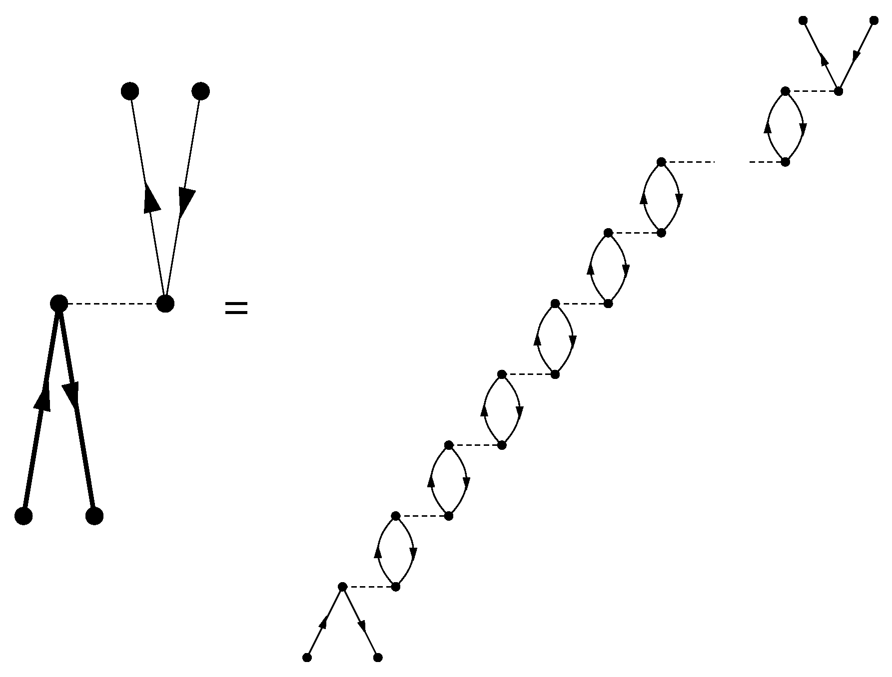
If we neglect the exchange term, we have a simple algebraic relation between the Green functions in momentum space

$$\begin{array}{ccc}& & {\tilde{G}}^{\mathrm{RPA},\mathrm{D}}(k_1,k_2;E)={\tilde{G}}^0(k_1,k_2;E)+{\tilde{G}}^0(k_1,k_2;E)\widetilde{\widehat{\mathcal{U}}}(k_1-k_2=q){\tilde{G}}^{\mathrm{RPA},\mathrm{D}}(k_1,k_2;E),\hfill \\ \hfill & & {\tilde{G}}^{\mathrm{RPA},\mathrm{D}}(k_1,k_1+q;E)\left[1-{\tilde{G}}^0(k_1,k_1+q;E)\widetilde{\widehat{\mathcal{U}}}\left(q\right)\right]={\tilde{G}}^0(k_1,k_1+q;E),\hfill \\ & & {\tilde{G}}^{\mathrm{RPA},\mathrm{D}}(k_1,k_1+q;E)=\frac{{\tilde{G}}^0(k_1,k_1+q;E)}{1-{\tilde{G}}^0(k_1,k_1+q;E)\widetilde{\widehat{\mathcal{U}}}\left(q\right)}.\hfill \end{array}$$

(132)

This expression is commonly used to calculate the linear response of infinite fermion systems to an external probe. The graphical representation of the above equation is given in Figure 5. The equation represents an infinite sum of diagrams of ring form and it is, therefore, called ring approximation.

The exchange term cannot be factorized as the direct one. The inclusion of this term is sometimes treated by using approximated treatments. One of them is the continuous fraction technique [26,27].

5. RPA with Time-Dependent Hartree–Fock

Another way of obtaining RPA secular Equation (67) is that of using time-dependent Hartree–Fock (TDHF) equations and the variational principle. We apply the variational principle to the time-dependent Schrödinger equation

$$\delta \langle \mathrm{\Psi }\left(t\right)|\left(\widehat{H}-i\hslash \frac{\partial }{\partial t}\right)|\mathrm{\Psi }\left(t\right)\rangle =0.$$

(133)

The search for the minimum of the above functional of $\mathrm{\Psi }\left(t\right)$ is carried out in the Hilbert subspace spanned by many-body wave functions of the form

$$|\mathrm{\Psi }\left(t\right)\rangle =e^{{\displaystyle \sum _{mi}{C}_{mi}\left(t\right){\widehat{a}}_m^{+}{\widehat{a}}_i}}|{\Phi }_0\left(t\right)\rangle ,$$

(134)

where the time-dependent IPM state has been defined as

$$|{\Phi }_0\left(t\right)\rangle =e^{-\frac{i}{\hslash }{\mathcal{E}}_{0}t}|{\Phi }_0\rangle .$$

(135)

In the above equation, $|{\Phi }_0\rangle$ is the stationary Hartree–Fock ground state of which ${\mathcal{E}}_0$, Equation (14), is the energy eigenvalue. In Equation (133), the variation of the real and of the imaginary part of $\mathrm{\Psi }\left(t\right)$ are independent. The variation is carried on the only time dependent terms which are $C_{mi}\left(t\right)$ and $C_{mi}^{*}\left(t\right)$. We obtain a system composed by the equations

$$\begin{array}{ccc}\hfill \frac{\delta }{\delta C_{mi}^{*}\left(t\right)}\langle \mathrm{\Psi }\left(t\right)|\widehat{H}-i\hslash \frac{\partial }{\partial t}|\mathrm{\Psi }\left(t\right)\rangle & =& 0,\hfill \end{array}$$

(136)

$$\begin{array}{ccc}\hfill \frac{\delta }{\delta C_{mi}\left(t\right)}\langle \mathrm{\Psi }\left(t\right)|\widehat{H}-i\hslash \frac{\partial }{\partial t}|\mathrm{\Psi }\left(t\right)\rangle & =& 0.\hfill \end{array}$$

(137)

We consider Equation (136) and calculate the expectation value of operators by using the power expansion of the exponential

$$e^{{\displaystyle \sum _{mi}{C}_{mi}\left(t\right){\widehat{a}}_m^{+}{\widehat{a}}_i}}=\widehat{\mathbb{I}}+\sum _{mi}{C}_{mi}\left(t\right){\widehat{a}}_m^{+}{\widehat{a}}_i+\frac{1}{2}\sum _{minj}{C}_{mi}\left(t\right){\widehat{a}}_m^{+}{\widehat{a}}_i{C}_{nj}\left(t\right){\widehat{a}}_n^{+}{\widehat{a}}_j+\cdots ,$$

(138)

For the hamiltonian expectation value, we obtain the expression

$$\begin{array}{ccc}\hfill \langle \mathrm{\Psi }\left(t\right)|\widehat{H}|\mathrm{\Psi }\left(t\right)\rangle & =& \langle {\Phi }_0\left(t\right)|\widehat{H}|{\Phi }_0\left(t\right)\rangle \hfill \\ \hfill & +& \sum _{mi}{C}_{mi}^{*}\left(t\right)\langle {\Phi }_0\left(t\right)|{\widehat{a}}_i^{+}{\widehat{a}}_m\widehat{H}|{\Phi }_0\left(t\right)\rangle \hfill \\ \hfill & +& \sum _{mi}{C}_{mi}\left(t\right)\langle {\Phi }_0\left(t\right)|\widehat{H}{\widehat{a}}_m^{+}{\widehat{a}}_i|{\Phi }_0\left(t\right)\rangle \hfill \\ \hfill & +& \frac{1}{2}\sum _{minj}{C}_{mi}^{*}\left(t\right)C_{nj}^{*}\left(t\right)\langle {\Phi }_0\left(t\right)|{\widehat{a}}_j^{+}{\widehat{a}}_n{\widehat{a}}_i^{+}{\widehat{a}}_m\widehat{H}|{\Phi }_0\left(t\right)\rangle \hfill \\ \hfill & +& \frac{1}{2}\sum _{minj}{C}_{mi}\left(t\right)C_{nj}\left(t\right)\langle {\Phi }_0\left(t\right)|\widehat{H}{\widehat{a}}_m^{+}{\widehat{a}}_i{\widehat{a}}_n^{+}{\widehat{a}}_j|{\Phi }_0\left(t\right)\rangle \hfill \\ & +& \sum _{minj}{C}_{mi}^{*}\left(t\right)C_{nj}\left(t\right)\langle {\Phi }_0\left(t\right)|{\widehat{a}}_i^{+}{\widehat{a}}_m\widehat{H}{\widehat{a}}_n^{+}{\widehat{a}}_j\widehat{H}|{\Phi }_0\left(t\right)\rangle +\cdots .\hfill \end{array}$$

(139)

The first term of the above equation is the ${\mathcal{E}}_0$ of Equation (14). The linear terms in $C_{mi}\left(t\right)$ are all zero since they overlap with orthogonal Slater determinants, or, in other words, since the number of $ph$ operators is odd.

Let us calculate the matrix element of the fifth term by using the expression of the hamiltonian given in Equation (12)

$$\begin{array}{ccc}\hfill & & \langle {\Phi }_0\left(t\right)|\widehat{H}{\widehat{a}}_m^{+}{\widehat{a}}_i{\widehat{a}}_n^{+}{\widehat{a}}_j|{\Phi }_0\left(t\right)\rangle =\sum _{\nu }{ϵ}_{\nu }\langle {\Phi }_0\left(t\right)|{\widehat{a}}_{\nu }^{+}{\widehat{a}}_{\nu }{\widehat{a}}_m^{+}{\widehat{a}}_i{\widehat{a}}_n^{+}{\widehat{a}}_j|{\Phi }_0\left(t\right)\rangle \hfill \\ \hfill & -& \frac{1}{2}\sum _{kl}{\overline{V}}_{klkl}\langle {\Phi }_0\left(t\right)|{\widehat{a}}_m^{+}{\widehat{a}}_i{\widehat{a}}_n^{+}{\widehat{a}}_j|{\Phi }_0\left(t\right)\rangle \hfill \\ & +& \frac{1}{4}\sum _{\mu {\mu }^{\prime }\nu {\nu }^{\prime }}{\overline{V}}_{\nu \mu {\nu }^{\prime }{\mu }^{\prime }}\langle {\Phi }_0\left(t\right)|\widehat{\mathbb{N}}\left[{\widehat{a}}_{\nu }^{+}{\widehat{a}}_{\mu }^{+}{\widehat{a}}_{{\mu }^{\prime }}{\widehat{a}}_{{\nu }^{\prime }}\right]{\widehat{a}}_m^{+}{\widehat{a}}_i{\widehat{a}}_n^{+}{\widehat{a}}_j|{\Phi }_0\left(t\right)\rangle .\hfill \end{array}$$

(140)

The first and second terms are zero because of the orthogonality of the Slater determinants. With a calculation analogous to that leading to the interacting term of $A_{minj}$ in Equation (68) (this calculation is presented in Equation (A19)), we obtain

$$\frac{1}{4}\sum _{\mu {\mu }^{\prime }\nu {\nu }^{\prime }}{\overline{V}}_{\nu \mu {\nu }^{\prime }{\mu }^{\prime }}\langle {\Phi }_0\left(t\right)|\widehat{\mathbb{N}}\left[{\widehat{a}}_{\nu }^{+}{\widehat{a}}_{\mu }^{+}{\widehat{a}}_{{\mu }^{\prime }}{\widehat{a}}_{{\nu }^{\prime }}\right]{\widehat{a}}_m^{+}{\widehat{a}}_i{\widehat{a}}_n^{+}{\widehat{a}}_j|{\Phi }_0\left(t\right)\rangle ={\overline{V}}_{ijmn}.$$

(141)

The fifth term of Equation (139) can be written as

$$\frac{1}{2}\sum _{minj}{C}_{mi}\left(t\right)C_{nj}\left(t\right)\langle {\Phi }_0\left(t\right)|\widehat{H}{\widehat{a}}_m^{+}{\widehat{a}}_i{\widehat{a}}_n^{+}{\widehat{a}}_j|{\Phi }_0\left(t\right)\rangle =\frac{1}{2}\sum _{minj}{C}_{mi}\left(t\right)C_{nj}\left(t\right){\overline{V}}_{ijmn}.$$

(142)

By working in an analogous manner for the fourth term of Equation (139), we obtain

$$\frac{1}{2}\sum _{minj}{C}_{mi}^{*}\left(t\right)C_{nj}^{*}\left(t\right)\langle {\Phi }_0\left(t\right)|{\widehat{a}}_j^{+}{\widehat{a}}_n{\widehat{a}}_i^{+}{\widehat{a}}_m\widehat{H}|{\Phi }_0\left(t\right)\rangle =\frac{1}{2}\sum _{minj}{C}_{mi}^{*}\left(t\right)C_{nj}^{*}\left(t\right){\overline{V}}_{mnij}.$$

(143)

The expression of the last term of Equation (139) is

$$\begin{array}{ccc}\hfill & & \sum _{minj}{C}_{mi}^{*}\left(t\right)C_{nj}\left(t\right)\langle {\Phi }_0\left(t\right)|{\widehat{a}}_i^{+}{\widehat{a}}_m\widehat{H}{\widehat{a}}_n^{+}{\widehat{a}}_j\widehat{H}|{\Phi }_0\left(t\right)\rangle \hfill \\ \hfill & =& \sum _{mi}|C_{mi}{|}^2\sum _k{ϵ}_k+\sum _{mi}{|C_{mi}|}^2({ϵ}_m-{ϵ}_i)\hfill \\ \hfill & & -\frac{1}{2}\sum _{mi}{|C_{mi}|}^2\sum _{kl}{\overline{V}}_{klkl}+\sum _{minj}{C}_{mi}{C}_{nj}^{*}{\overline{V}}_{mjin}\hfill \\ & \equiv & {\mathcal{E}}_0\sum _{mi}|C_{mi}{|}^2+\sum _{mi}{|C_{mi}|}^2({ϵ}_m-{ϵ}_i)+\sum _{minj}{C}_{mi}{C}_{nj}^{*}{\overline{V}}_{mjin},\hfill \end{array}$$

(144)

where we used the definition (14) of ${\mathcal{E}}_0$. The final expression of Equation (139) is then

$$\begin{array}{ccc}\hfill \langle \mathrm{\Psi }\left(t\right)|\widehat{H}|\mathrm{\Psi }\left(t\right)\rangle & =& {\mathcal{E}}_0\left(1+\sum _{mi}{|C_{mi}|}^2\right)+\sum _{mi}{|C_{mi}|}^2({ϵ}_m-{ϵ}_i)+\sum _{minj}{C}_{mi}{C}_{nj}^{*}{\overline{V}}_{mjin}\hfill \\ & & +\frac{1}{2}\sum _{minj}{C}_{mi}\left(t\right)C_{nj}\left(t\right){\overline{V}}_{ijmn}+\frac{1}{2}\sum _{minj}{C}_{mi}^{*}\left(t\right)C_{nj}^{*}\left(t\right){\overline{V}}_{mnij}.\hfill \end{array}$$

(145)

Let us calculate the second term of Equation (136), containing the time derivation. By considering the expression (134) of $|\mathrm{\Psi }\left(t\right)\rangle$, we have

$$i\hslash \langle \mathrm{\Psi }\left(t\right)|\frac{\partial }{\partial t}|\mathrm{\Psi }\left(t\right)\rangle ={\mathcal{E}}_0\langle \mathrm{\Psi }\left(t\right)|\mathrm{\Psi }(t)\rangle +i\hslash \sum _{mi}\frac{d}{dt}{C}_{mi}\left(t\right)\langle \mathrm{\Psi }\left(t\right)|{\widehat{a}}_m^{+}{\widehat{a}}_i|\mathrm{\Psi }\left(t\right)\rangle .$$

(146)

We make a power expansion of the exponential function in Equation (134) and obtain

$$\begin{array}{ccc}\hfill \langle \mathrm{\Psi }\left(t\right)|\mathrm{\Psi }(t)\rangle & =& \langle {\Phi }_0\left(t\right)|{\Phi }_0\left(t\right)\rangle \hfill \\ & +& \sum _{minj}{C}_{mi}^{*}\left(t\right)C_{nj}\left(t\right)\langle {\Phi }_0\left(t\right)|{\widehat{a}}_i^{+}{\widehat{a}}_m{\widehat{a}}_n^{+}{\widehat{a}}_j|{\Phi }_0\left(t\right)\rangle +\cdots ,\hfill \end{array}$$

(147)

and after the application of the Wick’s theorem

$$\langle \mathrm{\Psi }\left(t\right)|\mathrm{\Psi }(t)\rangle =1+\sum _{mi}{|C_{mi}\left(t\right)|}^2+\cdots .$$

(148)

The terms of first order in C are zero because of the odd number of $ph$ excitation pairs. By using the power expansion of the exponential to calculate the second term of Equation (146), we have

$$\langle \mathrm{\Psi }\left(t\right)|{\widehat{a}}_m^{+}{\widehat{a}}_i|\mathrm{\Psi }\left(t\right)\rangle =\sum _{nj}{C}_{nj}^{*}\langle {\Phi }_0\left(t\right)|{\widehat{a}}_j^{+}{\widehat{a}}_n{\widehat{a}}_m^{+}{\widehat{a}}_i|{\Phi }_0\left(t\right)\rangle +\cdots =C_{mi}^{*}+\cdots .$$

(149)

The term related to the time derivative becomes

$$i\hslash \langle \mathrm{\Psi }\left(t\right)|\frac{\partial }{\partial t}|\mathrm{\Psi }\left(t\right)\rangle ={\mathcal{E}}_0\left(1+\sum _{mi}{|C_{mi}\left(t\right)|}^2\right)+i\hslash \sum _{mi}{C}_{mi}^{*}\left(t\right)\frac{d}{dt}{C}_{mi}\left(t\right)+\cdots .$$

(150)

We put together the results of Equations (145) and (150); we consider terms up to the second order in C and obtain the expression

$$\begin{array}{ccc}\hfill \langle \mathrm{\Psi }\left(t\right)|\widehat{H}-i\hslash \frac{\partial }{\partial t}|\mathrm{\Psi }\left(t\right)\rangle & \simeq & \sum _{mi}{|C_{mi}\left(t\right)|}^2({ϵ}_m-{ϵ}_i)+\sum _{minj}{C}_{mi}{C}_{nj}^{*}{\overline{V}}_{mjin}\hfill \\ \hfill & +& \frac{1}{2}\sum _{minj}{C}_{mi}\left(t\right)C_{nj}\left(t\right){\overline{V}}_{ijmn}+\frac{1}{2}\sum _{minj}{C}_{mi}^{*}\left(t\right)C_{nj}^{*}\left(t\right){\overline{V}}_{mnij}\hfill \\ & -& i\hslash \sum _{mi}{C}_{mi}^{*}\left(t\right)\frac{d}{dt}{C}_{mi}\left(t\right).\hfill \end{array}$$

(151)

We have to impose the variational condition

$$\frac{\delta }{\delta C_{mi}^{*}\left(t\right)}\langle \mathrm{\Psi }\left(t\right)|\widehat{H}-i\hslash \frac{\partial }{\partial t}|\mathrm{\Psi }\left(t\right)\rangle =\frac{\partial }{\partial C_{mi}^{*}\left(t\right)}\langle \mathrm{\Psi }\left(t\right)|\widehat{H}-i\hslash \frac{\partial }{\partial t}|\mathrm{\Psi }\left(t\right)\rangle =0,$$

(152)

where the variational derivative has been changed in partial derivatives since the C’s are the only terms depending on time. By working out the derivative, we obtain the expression

$$C_{mi}\left(t\right)({ϵ}_m-{ϵ}_i)+\sum _{nj}{C}_{nj}^{*}{\overline{V}}_{mnij}+\sum _{nj}{C}_{nj}{\overline{V}}_{mjin}=i\hslash \sum _{mi}\frac{d}{dt}{C}_{mi}\left(t\right).$$

(153)

We consider harmonic oscillations around the ground state

$$C_{mi}\left(t\right)=X_{mi}{e}^{-i\omega t}+Y_{mi}{e}^{i\omega t}.$$

(154)

where X, Y and $\omega$ are real numbers. By inserting this expression in Equation (153) and separating the positive and negative frequencies, we obtain the system of equations

$$\begin{array}{ccc}\hfill X_{mi}({ϵ}_m-{ϵ}_i)+\sum _{nj}{\overline{V}}_{mjin}{X}_{nj}+\sum _{nj}{\overline{V}}_{mnij}{Y}_{nj}& =& \hslash \omega X_{mi},\hfill \end{array}$$

(155)

$$\begin{array}{ccc}\hfill Y_{mi}^{*}({ϵ}_m-{ϵ}_i)+\sum _{nj}{\overline{V}}_{mjin}{Y}_{nj}^{*}+\sum _{nj}{\overline{V}}_{mnij}{X}_{nj}^{*}& =& -\hslash {\omega }^{*}{X}_{mi},\hfill \end{array}$$

(156)

which is identical to Equation (67) where the A and B matrices have been defined by Equations (68) and (69).

6. Continuum RPA

If the excitation energy $\omega$ of the system is larger than $|{ϵ}_h|$, the particle lying on this state can be emitted and leave the system. In an atom, this effect produces a positive ion, in a nucleus a new nucleus with $A-1$ nucleons. The RPA approach which explicitly considers the emission of a particle is called Continuum RPA (CRPA), where continuum refers to the fact that for ${ϵ}_p>0$ the IPM Schrödinger equation has a continuous spectrum. In this case, the s.p. wave function has an asymptotically oscillating behavior.

In CRPA, the operator (54) defining the excited state is written as

$${\widehat{Q}}_{\nu }^{†}=\sum _{\left[p\right]h}\sum {\int }_{{ϵ}_p}\left[X_{ph}^{\nu }\left({ϵ}_p\right){\widehat{a}}_p^{†}\left({ϵ}_p\right){\widehat{a}}_h-Y_{ph}^{\nu }\left({ϵ}_p\right){\widehat{a}}_h^{†}{\widehat{a}}_p\left({ϵ}_p\right)\right],$$

(157)

where we have introduced the symbol

$$\sum {\int }_{{ϵ}_p}\equiv \sum _{{ϵ}_{\mathrm{F}}\le {ϵ}_p\le 0}+{\int }_0^{\infty }\mathrm{d}{ϵ}_p$$

(158)

to indicate a sum on the discrete energies and an integral on the continuum part of the spectrum. The symbol $\left[p\right]$ indicates the set of quantum numbers characterizing the particle state with the exclusion of the energy.

RPA secular Equation (67) with the continuum can be written as

$$\begin{array}{ccc}\hfill ({ϵ}_p-{ϵ}_h-\omega )X_{ph}^{\nu }\left({ϵ}_p\right)+& & \\ & & \sum _{\left[p^{\prime }\right]h^{\prime }}\sum {\int }_{{ϵ}_{p^{\prime }}}\left[{\overline{V}}_{p{h}^{\prime }h{p}^{\prime }}({ϵ}_p,{ϵ}_{p^{\prime }})X_{p^{\prime }{h}^{\prime }}^{\nu }\left({ϵ}_{p^{\prime }}\right)+{\overline{V}}_{p{p}^{\prime }h{h}^{\prime }}({ϵ}_p,{ϵ}_{p^{\prime }})Y_{p^{\prime }{h}^{\prime }}^{\nu }\left({ϵ}_{p^{\prime }}\right)\right]=0,\hfill \end{array}$$

(159)

$$\begin{array}{ccc}\hfill ({ϵ}_p-{ϵ}_h+\omega )Y_{ph}^{\nu }\left({ϵ}_p\right)+& & \\ & & \sum _{\left[p^{\prime }\right]h^{\prime }}\sum {\int }_{{ϵ}_{p^{\prime }}}\left[{\overline{V}}_{hp{p}^{\prime }{h}^{\prime }}({ϵ}_p,{ϵ}_{p^{\prime }})Y_{p^{\prime }{h}^{\prime }}^{\nu }\left({ϵ}_p\right)+{\overline{V}}_{h{h}^{\prime }p{p}^{\prime }}({ϵ}_p,{ϵ}_{p^{\prime }})X_{p^{\prime }{h}^{\prime }}^{\nu }\left({ϵ}_{p^{\prime }}\right)\right]=0.\hfill \end{array}$$

(160)

where we have explicitly written the dependences on the particle energies which are now continuous variables.

In order to discuss the implications related to the fact that ${ϵ}_p$ can assume a continuous set of values, it is useful to express the X and Y RPA amplitudes as:

$$\begin{array}{ccc}\hfill X_{ph}^{\nu }\left({ϵ}_p\right)& =& A_{ph}^{\nu }\delta ({ϵ}_p-{ϵ}_h-\omega )+\mathcal{P}\frac{B_{ph}^{X,\nu }\left({ϵ}_p\right)}{{ϵ}_p-{ϵ}_h-\omega },\hfill \end{array}$$

(161)

$$\begin{array}{ccc}\hfill Y_{ph}^{\nu }\left({ϵ}_p\right)& =& \frac{B_{ph}^{Y,\nu }\left({ϵ}_p\right)}{{ϵ}_p-{ϵ}_h+\omega }.\hfill \end{array}$$

(162)

When ${ϵ}_p$ assumes the value ${ϵ}_p={ϵ}_h+\omega$, in the integrals of (159) and (160), the X amplitudes have a pole. In the above expression, the contribution of the pole, multiplied by a constant $A_{ph}^{\nu }$, is separated from the principal part, indicated by $\mathcal{P}$.

The CRPA secular equations in terms of the new unknown can be written as

$$\begin{array}{ccc}\hfill B_{ph}^{X,\nu }\left({ϵ}_p\right)& +& \sum _{\left[p^{\prime }\right]h^{\prime }}\sum {\int }_{{ϵ}_{p^{\prime }}}\left[{\overline{V}}_{p{h}^{\prime }h{p}^{\prime }}({ϵ}_p,{ϵ}_{p^{\prime }})\frac{B_{p^{\prime }{h}^{\prime }}^{X,\nu }\left({ϵ}_{p^{\prime }}\right)}{{ϵ}_{p^{\prime }}-{ϵ}_{h^{\prime }}-\omega }+{\overline{V}}_{p{p}^{\prime }h{h}^{\prime }}({ϵ}_p,{ϵ}_{p^{\prime }})\frac{B_{p^{\prime }{h}^{\prime }}^{Y,\nu }\left({ϵ}_{p^{\prime }}\right)}{{ϵ}_{p^{\prime }}-{ϵ}_{h^{\prime }}+\omega }\right]\hfill \\ & =& -\sum _{\left[p^{\prime }\right]h^{\prime }}{\overline{V}}_{p{h}^{\prime }h{p}^{\prime }}({ϵ}_p,{ϵ}_{p^{\prime }})A_{p^{\prime }{h}^{\prime }}^{\nu }\delta ({ϵ}_{p^{\prime }}-{ϵ}_{h^{\prime }}-\omega ),\hfill \end{array}$$

(163)

$$\begin{array}{ccc}\hfill B_{ph}^{Y,\nu }\left({ϵ}_p\right)& +& \sum _{\left[p^{\prime }\right]h^{\prime }}\sum {\int }_{{ϵ}_{p^{\prime }}}\left[{\overline{V}}_{hp{p}^{\prime }{h}^{\prime }}({ϵ}_p,{ϵ}_{p^{\prime }})\frac{B_{p^{\prime }{h}^{\prime }}^{Y,\nu }\left({ϵ}_{p^{\prime }}\right)}{{ϵ}_{p^{\prime }}-{ϵ}_{h^{\prime }}+\omega }+{\overline{V}}_{h{h}^{\prime }p{p}^{\prime }}({ϵ}_p,{ϵ}_{p^{\prime }})\frac{B_{p^{\prime }{h}^{\prime }}^{X,\nu }\left({ϵ}_{p^{\prime }}\right)}{{ϵ}_{p^{\prime }}-{ϵ}_{h^{\prime }}-\omega }\right]\hfill \\ & =& -\sum _{\left[p^{\prime }\right]h^{\prime }}{\overline{V}}_{hp{p}^{\prime }{h}^{\prime }}({ϵ}_p,{ϵ}_{p^{\prime }})A_{p^{\prime }{h}^{\prime }}^{\nu }\delta ({ϵ}_{p^{\prime }}-{ϵ}_{h^{\prime }}-\omega ).\hfill \end{array}$$

(164)

The above equations indicate a system of linear equations whose unknowns are the B’s.

The continuum threshold, ${\omega }_{\mathrm{thr}}$, is the minimum value of the energy necessary to emit the particle, i.e., the absolute value of the s.p. energy of the hole state closest to the Fermi surface. For $\omega <{\omega }_{\mathrm{thr}}$, no particle can be emitted. In this case, all the $A_{p^{\prime }{h}^{\prime }}^{\nu }=0$; therefore, the system is homogeneous. Solutions, different from the trivial one, are obtained when the determinant of the known coefficients is zero. This happens for some specific values of the excitation energy $\omega$. Below the emission threshold, the CRPA equations predict a discrete spectrum of solutions. When $\omega >{\omega }_{\mathrm{thr}}$, some $ph$ pairs have enough energy to put the particle in the continuum, i.e., with ${ϵ}_p>0$. In the CRPA jargon these $ph$ pairs are called open channels. Obviously, the other $ph$ pairs where ${ϵ}_p<0$ are called closed channels. Every open channel generates a coefficient different from zero in the right hand side of Equations (163) and (164). The problem is defined by imposing boundary conditions, which is equivalent to saying that we have to select specific values of the $A_{ph}^{\nu }$ coefficients. The choice commonly adopted consists in imposing that the particle is emitted in a specific open channel, called elastic channel. This means

$$A_{ph}^{\nu }={\delta }_{p,p_0}{\delta }_{h,h_0},$$

(165)

where $p_0$ and $h_0$ are the quantum numbers characterizing the elastic channel. The sums in terms of the right hand sides of Equations (163) and (164) collapse to a single term. For each value of the excitation energy $\omega$, the system has to be solved a number of times equal to the number of open channels.

The solution of the CRPA system of equations can be obtained by solving directly the set of Equations (163) and (164). The s.p. particle wave functions in the continuum are obtained by solving the s.p. Schrödinger equation with asymptotically oscillating boundary conditions. This is the classical problem of a particle elastically scattered by a potential. This problem has to be solved for a set of ${ϵ}_p$ energy values mapping the continuum in such a way that the integral of Equation (158) is numerically stable. This means that ${ϵ}_p$ must reach values much larger than those of the excitation energy region one wants to investigate. The selection of the ${ϵ}_p$ values to obtain the s.p. wave function is not a simple problem to be solved. The various particles may have more or less sharp resonances and they have to be properly described by the choice of the ${ϵ}_p$ values mapping the continuum.

There is another technical problem in the direct approach to the solution of the CRPA Equations (163) and (164). The numerical stability of the interaction matrix elements $\overline{V}$ is due to the fact that, in the integrals, hole wave functions, which asymptotically go to zero, are present. This works well for the direct matrix elements

$$\langle p_1{h}_2|\widehat{V}|h_1{p}_2\rangle =\int d^3{r}_1\int d^3{r}_2{\varphi }_{p_1}^{*}\left({\mathbf{r}}_1\right){\varphi }_{h_2}^{*}\left({\mathbf{r}}_2\right)V({\mathbf{r}}_1,{\mathbf{r}}_2){\varphi }_{h_1}\left({\mathbf{r}}_1\right){\varphi }_{p_2}\left({\mathbf{r}}_2\right),$$

(166)

but it is a problem for the exchange matrix element

$$\langle p_1{h}_2|\widehat{V}|p_2{h}_1\rangle =\int d^3{r}_1\int d^3{r}_2{\varphi }_{p_1}^{*}\left({\mathbf{r}}_1\right){\varphi }_{h_2}^{*}\left({\mathbf{r}}_2\right)V({\mathbf{r}}_1,{\mathbf{r}}_2){\varphi }_{p_2}\left({\mathbf{r}}_1\right){\varphi }_{h_1}\left({\mathbf{r}}_2\right),$$

(167)

where the two particle wave functions, both oscillating, are integrated together. The direct approach is suitable to be used with zero-range interactions $V({\mathbf{r}}_1,{\mathbf{r}}_2)=V_0\delta ({\mathbf{r}}_1-{\mathbf{r}}_2)$. In this case, direct and exchange matrix elements are identical

$$\langle p_1{h}_2|\widehat{V}|h_1{p}_2\rangle =\langle p_1{h}_2|\widehat{V}|p_2{h}_1\rangle =V_0\int d^3{r}_1{\varphi }_{p_1}^{*}\left({\mathbf{r}}_1\right){\varphi }_{h_2}^{*}\left({\mathbf{r}}_1\right){\varphi }_{p_2}\left({\mathbf{r}}_1\right){\varphi }_{h_1}\left({\mathbf{r}}_1\right),$$

(168)

and the hole wave functions are always present in the integral. This ensures the numerical convergence. The direct approach is used, for example, in Refs. [28,29], where the CRPA equations are expanded on a Fourier–Bessel basis.

Another method of solving the CRPA equations consists in reformulating the secular Equations (159) and (160) with new unknown functions which do not have explicit dependence on the continuous particle energy ${ϵ}_p$. The new unknowns are the channel functions f and g defined as:

$$f_{ph}^{\nu }\left(\mathbf{r}\right)=\sum {\int }_{{ϵ}_p}{X}_{ph}^{\nu }\left({ϵ}_p\right){\varphi }_p(\mathbf{r},{ϵ}_p),$$

(169)

and

$$g_{ph}^{\nu }\left(\mathbf{r}\right)=\sum {\int }_{{ϵ}_p}{Y}_{ph}^{\nu *}\left({ϵ}_p\right){\varphi }_p(\mathbf{r},{ϵ}_p).$$

(170)

In the first step of this procedure, we multiply Equations (163) and (164) by ${\varphi }_p(\mathbf{r},{ϵ}_p)$, which is the eigenfunction of the s.p. hamiltonian

$$\widehat{h}{\varphi }_p(\mathbf{r},{ϵ}_p)={ϵ}_p{\varphi }_p(\mathbf{r},{ϵ}_p),$$

(171)

and we obtain

$$({ϵ}_p-{ϵ}_h-\omega ){\varphi }_p(\mathbf{r},{ϵ}_p)X_{ph}^{\nu }\left({ϵ}_p\right)=\widehat{h}{\varphi }_p(\mathbf{r},{ϵ}_p)X_{ph}^{\nu }\left({ϵ}_p\right)-({ϵ}_h+\omega ){\varphi }_p(\mathbf{r},{ϵ}_p)X_{ph}^{\nu }\left({ϵ}_p\right).$$

(172)

Since the s.p. hamiltonian $\widehat{h}$ does not depend on ${ϵ}_p$, we can write

$$\sum {\int }_{{ϵ}_p}\widehat{h}{\varphi }_p(\mathbf{r},{ϵ}_p)X_{ph}^{\nu }\left({ϵ}_p\right)=\widehat{h}{f}_{ph}^{\nu }\left(\mathbf{r}\right).$$

(173)

We apply this procedure, i.e., multiplication of ${\varphi }_p\left(\mathbf{r}\right)$ and integration on ${ϵ}_p$, to all the terms of Equations (159) and (160). By considering that

$$\int d{ϵ}_p{\varphi }_p^{*}\left({\mathbf{r}}_1\right){\varphi }_p\left({\mathbf{r}}_2\right)=\delta ({\mathbf{r}}_1-{\mathbf{r}}_2),$$

we obtain a new set of CRPA secular equations where the unknowns are the channel functions f and g,

$$\begin{array}{ccc}\hfill \widehat{h}{f}_{ph}\left(\mathbf{r}\right)-({ϵ}_h+\omega )f_{ph}\left(\mathbf{r}\right)& =& -{\mathcal{F}}_{ph}\left(\mathbf{r}\right)\hfill \\ & +& \sum _{{ϵ}_p<{ϵ}_{\mathrm{F}}}{\varphi }_p\left(\mathbf{r}\right)\int {\mathrm{d}}^3{r}_1{\varphi }_h^{*}\left({\mathbf{r}}_1\right){\mathcal{F}}_{ph}\left({\mathbf{r}}_1\right),\hfill \end{array}$$

(174)

$$\begin{array}{ccc}\hfill \widehat{h}{g}_{ph}\left(\mathbf{r}\right)-({ϵ}_h-\omega )g_{ph}\left(\mathbf{r}\right)& =& -{\mathcal{G}}_{ph}\left(\mathbf{r}\right)\hfill \\ & +& \sum _{{ϵ}_p<{ϵ}_{\mathrm{F}}}{\varphi }_p\left(\mathbf{r}\right)\int {\mathrm{d}}^3{r}_1{\varphi }_h^{*}\left({\mathbf{r}}_1\right){\mathcal{G}}_{ph}\left({\mathbf{r}}_1\right),\hfill \end{array}$$

(175)

where we have defined

$$\begin{array}{ccc}\hfill {\mathcal{F}}_{ph}\left(r\right)& =& \sum _{\left[p^{\prime }\right]h^{\prime }}\int {\mathrm{d}}^3{r}_{2}V(\mathbf{r},{\mathbf{r}}_2)\{{\varphi }_{h^{\prime }}^{*}\left({\mathbf{r}}_2\right)\left[{\varphi }_h\left(\mathbf{r}\right)f_{p^{\prime }{h}^{\prime }}\left({\mathbf{r}}_2\right)-f_{p^{\prime }{h}^{\prime }}\left(\mathbf{r}\right){\varphi }_h\left({\mathbf{r}}_2\right)\right]\hfill \\ & +& g_{p^{\prime }{h}^{\prime }}^{*}\left({\mathbf{r}}_2\right)\left[{\varphi }_h\left(\mathbf{r}\right){\varphi }_{h^{\prime }}\left({\mathbf{r}}_2\right)-{\varphi }_{h^{\prime }}\left(\mathbf{r}\right){\varphi }_h\left({\mathbf{r}}_2\right)\right]\},\hfill \end{array}$$

(176)

and ${\mathcal{G}}_{ph}$ is obtained from the above equation by interchanging the f and g channel functions. The last terms of both Equations (174) and (175) are the contributions of particle wave functions ${\varphi }_p$ which are not in the continuum.

We changed a set of algebraic equations with unknowns depending on the continuous variable ${ϵ}_p$ into a set of integro-differential equations whose unknowns depend on $\mathbf{r}$. In analogy to what we have discussed above, for the direct solution of the CRPA secular equations, we solve Equations (174) and (175) a number of times equal to the number of the open channels, by imposing that the particle is emitted only in the elastic channel.

In spherical systems, the boundary conditions are imposed on the radial parts of the f and g functions. For an open $ph$ channel, the outgoing asymptotic behavior of the channel function $f_{ph}^{p_0{h}_0}$ is

$$f_{ph}^{p_0{h}_0}(r\to \infty )\to R_{p_0}(r,{ϵ}_p){\delta }_{p,p_0}{\delta }_{h,h_0}+\lambda H_p^{-}({ϵ}_h+\omega ,r),$$

(177)

where $\lambda$ is a complex normalization constant and $H_p^{-}({ϵ}_h+\omega ,r)$ is an ingoing Coulomb function if the emitted particle is electrically charged or a Hankel function in cases of neutron. The radial part of the s.p. wave function $R_p$ is the eigenfunction of the s.p. hamiltonian for positive energy. In the case of a closed channel, the asymptotic behavior is given by a decreasing exponential function

$$f_{ph}^{p_0{h}_0}(r\to \infty )\to \frac{1}{r}exp\left[-r{\left(\frac{2m|{ϵ}_h+\omega |}{{\hslash }^2}\right)}^{\frac{1}{2}}\right],$$

(178)

in analogy to the case of the channel functions $g_{ph}^{p_0{h}_0}$,

$$g_{ph}^{p_0{h}_0}(r\to \infty )\to \frac{1}{r}exp\left[-r{\left(\frac{2m|{ϵ}_h-\omega |}{{\hslash }^2}\right)}^{\frac{1}{2}}\right].$$

(179)

This approach solves the two technical problems of the direct approach indicated above, since the integration ${ϵ}_p$ is formally done in the definition of the two channel functions f and g.

These CRPA secular equations can be solved by using a procedure similar to that presented in Refs. [30,31]. The channel functions f and g are expanded on the basis of Sturm functions ${\Phi }_p^{\mu }$ which obey the required boundary conditions (177)–(179).

In the IPM, the particle emission process is described by considering that a particle lying on the hole state $h_0$ is emitted in the particle state $p_0$. The CRPA considers this fact in the elastic channel and, in addition, takes care of the fact that the residual interaction mixes this direct emission with all the other $ph$ pairs compatible with the total angular momentum of the excitation.

7. Quasi-Particle RPA (QRPA)

In the derivations presented in the previous sections, we considered that the IPM ground state is defined by a unique Slater determinant $|{\Phi }_0\rangle$, where all the s.p. states below the Fermi energy are fully occupied and those above it are completely empty. This description does not consider the presence of an effect which is very important in nuclei: the pairing. This effect couples two like-fermions to form a unique bosonic system. In metals this produces the effects of superconductivity. In nuclear physics this leads to the fact that all the even–even nuclei, without exceptions, have spin zero.

A convenient description of pairing effects is based on the Bardeen–Cooper–Schrieffer (BCS) theory of superconductivity [32]. In this approach, the choice of $|{\Phi }_0\rangle$ for the description of the system ground state is abandoned.

Let us consider a finite fermion system and use the expression Equation (8) for the s.p. wave functions. We introduce a notation to indicate time-reversed s.p. wave functions

$$|k\rangle :=|nl\frac{1}{2}jm\rangle ;|-k\rangle :=|nl\frac{1}{2}j-m\rangle .$$

(180)

The BCS ground state is defined as

$$|\mathrm{BCS}\rangle :=\prod _{k>0}^{\infty }\left(u_k+v_k{\widehat{a}}_k^{+}{\widehat{a}}_{-k}^{+}\right)|-\rangle ,$$

(181)

where we have indicated with $|-\rangle$ the state describing the physical vacuum. The $v_k^2$ factor is the occupation probability of the k-th s.p. state, and $u_k^2=1-v_k^2$ the probability of being empty. When pairing effects are negligible, for example, in doubly magic nuclei, $v_k=1$ for all the s.p. states below the Fermi surface and $v_k=0$ for all the states above it; therefore, $|\mathrm{BCS}\rangle =|{\Phi }_0\rangle$.

A convenient manner of handling the $|\mathrm{BCS}\rangle$ states is to define quasi-particle creation and destruction operators which are linear combinations of usual particle creation and destruction operators. The relations are known as Bogoliubov–Valatin transformations

$$\begin{array}{ccc}\hfill {\widehat{\alpha }}_k& =& u_k{\widehat{a}}_k-v_k{\widehat{a}}_{-k}^{+},\hfill \end{array}$$

(182)

$$\begin{array}{ccc}\hfill {\widehat{\alpha }}_k^{+}& =& u_k{\widehat{a}}_k^{+}-v_k{\widehat{a}}_{-k}.\hfill \end{array}$$

(183)

Since the quasi-particle operators are linear combination of the creation and destruction operators, anti-commutation relations analogous to (A3) are valid also for the $\widehat{\alpha }$ and ${\widehat{\alpha }}^{+}$ operators. It is possible to show that [14]

$${\widehat{\alpha }}_k|\mathrm{BCS}\rangle =0,$$

(184)

indicating that the $|\mathrm{BCS}\rangle$ states can be appropriately called quasi-particle vacuum. The BCS ground state is not an eigenstate of the number operator

$$\widehat{N}=\sum _k{\widehat{a}}_k^{+}{\widehat{a}}_k,$$

(185)

and the number of particles is conserved only on average [13,14]

$$\langle \mathrm{BCS}|\widehat{N}|\mathrm{BCS}\rangle =2\sum _{k>0}{v}_k^2=A.$$

(186)

The values of the $v_k$ coefficients, and consequently those of $u_k$, are obtained by exploiting the variational principle. For this reason, it is common practice to use a definition of the hamiltonian containing the Lagrange multiplier $\lambda$, related to the total number of particle A

$$\widehat{\mathcal{H}}=\widehat{H}-\lambda \widehat{N}.$$

(187)

The hamiltonian $\widehat{H}$ is written by expressing in Equation (A13) the $\widehat{a}$ and ${\widehat{a}}^{+}$ operators in terms of the quasi-particle operators ${\alpha }^{+}$ and $\alpha$. By observing the operator structure, it is possible to identify four different terms (see Equation (13.32) of [14])

$$\widehat{\mathcal{H}}=\widehat{H}-\lambda \widehat{N}={\widehat{\mathcal{H}}}_0+{\widehat{\mathcal{H}}}_{11}+{\widehat{\mathcal{H}}}_{22}+{\widehat{H}}_{\mathrm{int}},$$

(188)

where $\lambda$ is present only in the first three terms. The various terms are defined as follows.

• ${\widehat{\mathcal{H}}}_0$ is purely scalar,

  $${\widehat{\mathcal{H}}}_0=\sum _k\left[({ϵ}_k-\lambda -{\mu }_k)2v_k^2+u_k{v}_k\sum _{k^{\prime }}{\overline{V}}_{k,k^{\prime },k,k^{\prime }}{u}_{k^{\prime }}{v}_{k^{\prime }}\right].$$

  (189)
• ${\widehat{\mathcal{H}}}_{11}$ depends on ${\widehat{\alpha }}_k^{+}{\widehat{\alpha }}_k$,

  $${\widehat{\mathcal{H}}}_{11}=\sum _k\left\{\left[{ϵ}_k-\lambda -{\mu }_k\right](u_k^2-v_k^2)+2u_k{v}_k{\Delta }_k\right\}{\widehat{\alpha }}_k^{+}{\widehat{\alpha }}_k.$$

  (190)
• ${\widehat{\mathcal{H}}}_{22}$ depends on $\widehat{\mathbb{N}}[{\widehat{\alpha }}_k^{+}{\widehat{\alpha }}_{k^{\prime }}^{+}+{\widehat{\alpha }}_k{\widehat{\alpha }}_{k^{\prime }}]$.
• ${\widehat{H}}_{\mathrm{int}}={\widehat{H}}_{40}+{\widehat{H}}_{31}+{\widehat{H}}_{22}$, where
  • ${\widehat{H}}_{40}$ depends on $[{\widehat{\alpha }}_{k_1}^{+}{\widehat{\alpha }}_{k_2}^{+}{\widehat{\alpha }}_{k_3}^{+}{\widehat{\alpha }}_{k_4}^{+}+h.c.]$,
  • ${\widehat{H}}_{31}$ depends on $[{\widehat{\alpha }}_{k_1}^{+}{\widehat{\alpha }}_{k_2}^{+}{\widehat{\alpha }}_{k_3}^{+}{\widehat{\alpha }}_{k_4}+h.c.]$,
  • and finally,

    $${\widehat{H}}_{22}=\frac{1}{2}\sum _{abcd}{V}_{abcd}^{\left(22\right)}{\widehat{\alpha }}_{k_a}^{+}{\widehat{\alpha }}_{k_b}^{+}{\widehat{\alpha }}_{k_d}{\widehat{\alpha }}_{k_c},$$

    (191)

    with

    $$V_{abcd}^{\left(22\right)}=(u_a{u}_b{u}_c{u}_d+v_a{v}_b{v}_c{v}_d+4u_a{v}_b{u}_c{v}_d){\overline{V}}_{abcd}.$$

    (192)

In the above equations, we used the following scalar quantities:

$$\begin{array}{ccc}\hfill {\Delta }_k& =& -\sum _{k^{\prime }}{\overline{V}}_{k,-k,k^{\prime },-k^{\prime }}{u}_{k^{\prime }}{v}_{k^{\prime }},\hfill \end{array}$$

(193)

$$\begin{array}{ccc}\hfill {ϵ}_k& =& \int d^{3}r{\varphi }_k^{*}\left(\mathbf{r}\right)\left(\frac{-{\hslash }^2{\nabla }^2}{2m}\right){\varphi }_k\left(\mathbf{r}\right)+\frac{1}{2}\sum _{k^{\prime }}{\overline{V}}_{k,k^{\prime },k,k^{\prime }}{v}_{k^{\prime }}^2,\hfill \end{array}$$

(194)

$$\begin{array}{ccc}\hfill {\mu }_k& =& -\frac{1}{2}\sum _{k^{\prime }}{\overline{V}}_{k,k^{\prime },k,k^{\prime }}{v}_{k^{\prime }}^2.\hfill \end{array}$$

(195)

Because of Equation (184) the expectation value of $\widehat{\mathcal{H}}$ with respect to the BCS ground state is

$$\langle BCS|\widehat{\mathcal{H}}|BCS\rangle =\langle BCS|{\widehat{\mathcal{H}}}_0|BCS\rangle \equiv {\mathcal{E}}_A^{\mathrm{BCS}};$$

(196)

therefore, the application of the variational principle is

$$\delta \left(\langle BCS|{\widehat{\mathcal{H}}}_0|BCS\rangle \right)=0,$$

(197)

which implies the relation [13,14]:

$$(u^2-v^2){\Delta }_k=2v_k{u}_k({ϵ}_k-\lambda +{\mu }_k)\Rightarrow v_k{u}_k=\frac{{\Delta }_k}{2\sqrt{{({ϵ}_k-\lambda -{\mu }_k)}^2+{\Delta }_k^2}}.$$

(198)

We insert the above result in Equation (190) and obtain the BCS s.p. energies

$${\widehat{\mathcal{H}}}_{11}=\left\{\sqrt{{({ϵ}_k-\lambda -{\mu }_k)}^2+{\Delta }_k^2}\right\}{\widehat{\alpha }}_k^{+}{\widehat{\alpha }}_k:={ϵ}_k^{\mathrm{BCS}}{\widehat{\alpha }}_k^{+}{\widehat{\alpha }}_k.$$

(199)

In the BCS approach, the radial expressions of the s.p. wave functions are obtained by carrying out IPM calculations and only the occupation amplitudes $v_k$ and $u_k$ are modified. There is a more fundamental approach, the Hartree–Fock–Bogolioubov theory, where s.p. wave functions, energies and occupation probabilities are calculated in a unique theoretical framework whose only input is the effective nucleon–nucleon interaction.

After having defined a new ground state containing pairing effects, we can use it to develop the theory describing the harmonic vibrations around it. The derivation of the QRPA secular equations is carried out by using the EOM method described in Section 3. In this case, the Slater determinant $|{\Phi }_0\rangle$ is substituted by the BCS ground state $|\mathrm{BCS}\rangle$ and the particle creation and destruction operators ${\widehat{a}}_k$ and ${\widehat{a}}_k^{+}$ by the quasi-particle operators ${\widehat{\alpha }}_k$ and ${\widehat{\alpha }}_k^{+}$. The QRPA excitation operator is given by

$$Q_{\nu }^{+}\equiv \sum _{a\le b}{X}_{ab}^{\nu }{\widehat{\alpha }}_a^{+}{\widehat{\alpha }}_b^{+}-\sum _{a\le b}{Y}_{ab}^{\nu }{\widehat{\alpha }}_a{\widehat{\alpha }}_b.$$

(200)

The indexes a and b containing all the quantum numbers which identify the quasi-particle states are not, any more, referred to as particle or hole states. In this approach, the idea of Fermi surface has disappeared. Each quasi-particle state can be partially occupied. For this reason, in the above equation, we had to impose restrictions on the sums in order to avoid double counting.

In the present case, the EOM (39) assumes the expression

$$\langle \mathrm{BCS}|\left[\delta {\widehat{Q}}_{\nu },[\widehat{\mathcal{H}},{\widehat{Q}}_{\nu }^{+}]\right]|\mathrm{BCS}\rangle =\omega \langle \mathrm{BCS}|\left[\delta {\widehat{Q}}_{\nu },{\widehat{Q}}_{\nu }^{+}\right]|\mathrm{BCS}\rangle ,$$

(201)

where we have substituted $\widehat{\mathcal{O}}$ with $\delta {\widehat{Q}}_n$. Following the steps of the derivation of RPA equations, see Section 3.2, and defining A and B matrices as

$$\begin{array}{ccc}\hfill A_{ab,cd}& \equiv & \langle \mathrm{BCS}|\left[{\widehat{\alpha }}_a{\widehat{\alpha }}_b,[\widehat{\mathcal{H}},{\widehat{\alpha }}_c^{+}{\widehat{\alpha }}_d^{+}]\right]|\mathrm{BCS}\rangle ,\hfill \end{array}$$

(202)

$$\begin{array}{ccc}\hfill B_{ab,cd}& \equiv & -\langle \mathrm{BCS}|\left[{\widehat{\alpha }}_a{\widehat{\alpha }}_b,[\widehat{\mathcal{H}},{\widehat{\alpha }}_c{\widehat{\alpha }}_d]\right]|\mathrm{BCS}\rangle ,\hfill \end{array}$$

(203)

it is possible to obtain a set of linear equations analogous to those of RPA

$$\begin{array}{ccc}\hfill \sum _{c\le d}{A}_{ab,cd}{X}_{cd}^{\nu }+\sum _{c\le d}{B}_{ab,cd}{Y}_{cd}^{\nu }& =& {\omega }_{\nu }{X}_{ab}^{\nu },\hfill \end{array}$$

(204)

$$\begin{array}{ccc}\hfill \sum _{c\le d}{B}_{cd,ab}^{*}{X}_{cd}^{\nu }+\sum _{c\le d}{A}_{cd,ab}{Y}_{cd}^{\nu }& =& -{\omega }_{\nu }{Y}_{ab}^{\nu },\hfill \end{array}$$

(205)

which can be written in matrix form analogously to Equation (67). This calculation is explicitly carried out in Chapter 18 of Ref. [14] and it shows that only ${\widehat{\mathcal{H}}}_0$, ${\widehat{\mathcal{H}}}_{11}$ and ${\widehat{\mathcal{H}}}_{22}$ contribute to the A and B matrices. These matrices contain, in addition to the particle–hole excitations present in the common RPA, also particle–particle and hole–hole transitions, since each s.p. state is only partially occupied. The solution of the QRPA secular equations, for each excited state, provides the X and Y amplitudes which indicate the contribution of each quasi-particle excitation pair.

The QRPA solutions have the same properties of those of RPA solutions. The QRPA equations allow positive and negative eigenergies with the same absolute value. Eigenvectors corresponding to different energy eigenvalues are orthogonal. The set of QRPA eigenstates is complete.

The transition amplitudes from the QRPA ground state to an excited state, induced by an external one-body operator $\widehat{F}$, Equation (50), is

$$\langle \mathrm{QRPA};\nu |\widehat{F}|\mathrm{QRPA};0\rangle =\sum _{a\le b}{f}_{ab}\left(v_a{u}_b+u_a{v}_b\right)(X_{ab}^{\nu }+Y_{ab}^{\nu }).$$

(206)

For $ph$ transitions only, when $v_a=1,u_a=0$ and $v_b=0,u_b=1$ one recovers the ordinary RPA expression (74).

8. Specific Applications

In this section, I discuss some pragmatic issues arising in actual RPA calculations. The input of RPA calculations is composed by the s.p. energies and wave functions and also by the effective interaction between the particles forming the system. There are various possible choices of these quantities and they define different types of calculations.

A fully phenomenological approach is based on the Landau–Migdal theory of finite Fermi systems [33,34]. In this theory, the attention is concentrated on the small vibrations on top of the ground state, which is assumed to be perfectly known. The s.p. wave functions are generated by solving the MF Equation (4) with a phenomenological potential whose parameters are chosen to reproduce at best the empirical values of the s.p. energies of the levels around the Fermi surface. In RPA calculations, these empirical values are used when available; otherwise, the s.p. energies obtained by solving the MF equation are considered. The interaction is a zero-range density dependent Landau–Migdal force whose parameters are selected to reproduce some empirical characteristics of the excitation spectrum.

This approach has shown a great capacity to describe features of the excited states and also a remarkable predictive power. For example, the presence of a collective monopole excitation in ${}^{208}$Pb was predicted at the right energy [35] before it was identified by experiments with $\alpha$ [36] and ${}^3$He scattering [37]. The drawback consists in the need for a continuous tuning of the MF potential and the interaction parameters, since the results strongly depend on the input. This means that there is a set of force parameters for each nucleus, and also in the same nucleus the values of these parameters change if the dimensions of the configuration space are modified.

An approach which avoids this continuous setting of the free parameters is the so-called self-consistent approach. In this case, the s.p. wave functions and energies are generated by solving HF or DFT equations. The parameters of the effective interaction are tuned to reproduce at best experimental binding energies and charge radii, all along the isotope table. The same interaction, unique for all the nuclei, is used also in RPA calculations.

The density dependent zero-range Skyrme force is probably the interaction most used in this type of calculation [38]. The zero-range characteristic allows great simplifications of the expressions of the interaction matrix elements and the numerical calculations are relatively fast. There are tens of different sets of parameters of the Skyrme force, each of them properly tuned to describe some specific characteristics of the nuclei. The zero-range feature of the Skyrme force is mitigated by the presence of momentum dependent terms. On the other hand, the sensitivity on the dimensions of the s.p. configuration space is not negligible. For this reason, in BCS and QRPA calculations it is necessary to use a different interaction to treat the pairing.

These drawbacks are overcome by interactions which have finite range, a feature which clearly makes much more involved the numerical calculations. A widely used finite-range interaction is that of Gogny [39]. Despite this difference, the philosophy of the calculations carried out with the two kinds of interaction is the same: a unique force, valid all along the nuclide chart, tuned to reproduce ground state properties with HF calculations and used in RPA. Discrete RPA calculations carried out with Gogny force show a convergence of the results after certain dimensions of the configuration space have been reached.

The self-consistent approach does not provide an accurate description of the excited states obtained with the phenomenological approach. On the other hand, by using self-consistent approaches it is possible to make connections between the properties of the ground and of the excited state and also between features appearing in different nuclei, everything described within a unique theoretical framework. This approach can make predictions on properties of nuclei far from stability where empirical quantities have not yet been measured.

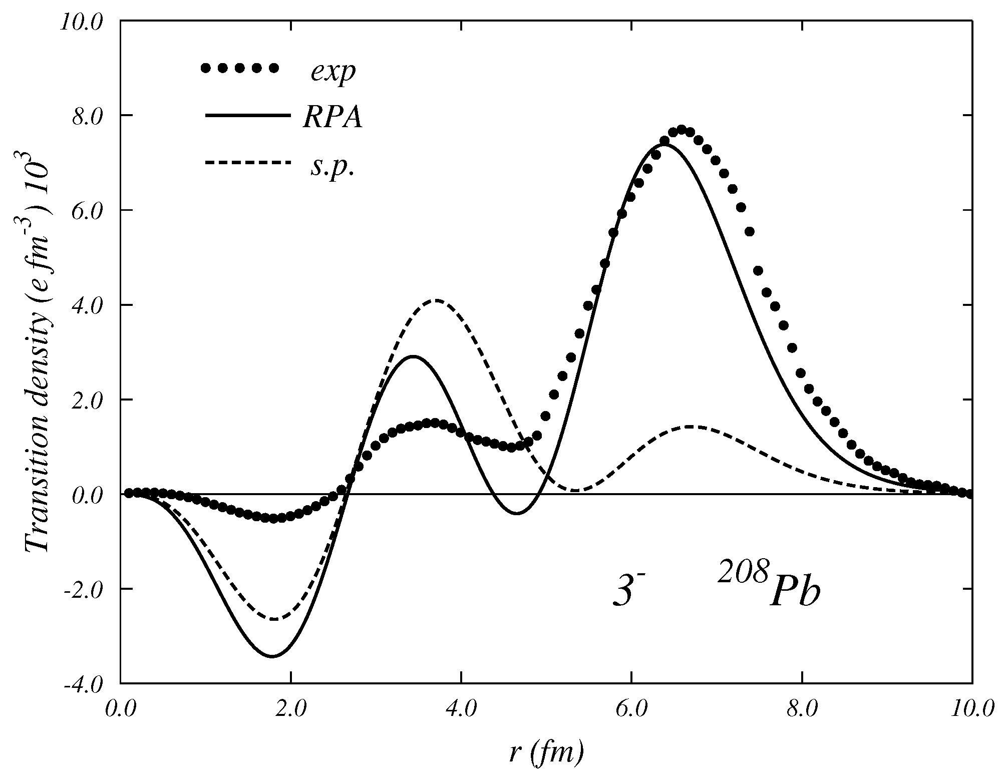
As an example of the RPA result, we consider the case of the $3^{-}$ state in ${}^{208}$Pb already mentioned in Section 2.4. We show in Figure 6 a comparison between the transition densities calculated with an RPA theory (full line), that obtained by an s.p. transition (dashed lines) and the empirical transition density (dots) extracted from the inelastic electron scattering data of Ref. [40]. The s.p. excitation was obtained by considering the proton transition from the $1s_{1/2}$ hole state to the $2f_{7/2}$ particle state with the excitation energy of 5.29 MeV. RPA calculation was carried out with the phenomenological approach and the excitation energy is of 2.66 MeV to be compared with an experimental value of 2.63 MeV.

The s.p. transition, which is what the IPM at its best can provide, is unable to describe the large values of the transition density at the nuclear surface. This surface vibration is a characteristic feature of this highly collective state. RPA is able to reproduce the value of the excitation energy and also the correct behavior of the transition density.

9. Extensions of RPA

9.1. Second RPA

The main limitation of RPA theory is due to the fact that the ${\widehat{Q}}_{\nu }^{+}$ operator considers only $1p-1h$ and $1h-1p$ types of excitations, see Equation (54). The many-body system allows more complicated excitation modes where n-particle and n-holes are created. The extension of ${\widehat{Q}}_{\nu }^{+}$ to consider also $2p-2h$ excitations is called Second RPA (SRPA) [41,42,43]. In this theory, the operator which defines the excited states is

$$\begin{array}{ccc}\hfill {\widehat{Q}}_{\nu }^{+}& \equiv & \sum _{m,i}\left(X_{mi}^{\nu }{\widehat{a}}_m^{+}{\widehat{a}}_i-Y_{mi}^{\nu }{\widehat{a}}_i^{+}{\widehat{a}}_m\right)\hfill \\ & +& \sum _{m<n,i<j}\left(X_{mnij}^{\nu }{\widehat{a}}_m^{+}{\widehat{a}}_n^{+}{\widehat{a}}_i{\widehat{a}}_j-Y_{mnij}^{\nu }{\widehat{a}}_i^{+}{\widehat{a}}_j^{+}{\widehat{a}}_m{\widehat{a}}_n\right)+\sum _{m,n,i,j}{Z}_{mjin}^{\nu }{\widehat{a}}_m^{+}{\widehat{a}}_j^{+}{\widehat{a}}_n{\widehat{a}}_i.\hfill \end{array}$$

(207)

where the X, Y and Z factors are real numbers.

We insert this operator into the EOM Equation (39) and substitute $\widehat{\mathcal{O}}$ with $\delta {\widehat{Q}}_{\nu }$. Since $\delta {\widehat{Q}}_{\nu }$ implies variations of the coefficients in (207) and these variations are independent of each other, we obtain five equations

$$\begin{array}{ccc}\hfill \langle \mathrm{RPAII}|\left[{\widehat{a}}_i^{+}{\widehat{a}}_m,[\widehat{H},{\widehat{Q}}_{\nu }^{+}]\right]|\mathrm{RPAII}\rangle & =& {\omega }_{\nu }\langle \mathrm{RPAII}|\left[{\widehat{a}}_i^{+}{\widehat{a}}_m,{\widehat{Q}}_{\nu }^{+}\right]|\mathrm{RPAII}\rangle ,\hfill \end{array}$$

(208)

$$\begin{array}{ccc}\hfill \langle \mathrm{RPAII}|\left[{\widehat{a}}_m^{+}{\widehat{a}}_i,[\widehat{H},{\widehat{Q}}_{\nu }^{+}]\right]|\mathrm{RPAII}\rangle & =& {\omega }_{\nu }\langle \mathrm{RPAII}|\left[{\widehat{a}}_m^{+}{\widehat{a}}_i,{\widehat{Q}}_{\nu }^{+}\right]|\mathrm{RPAII}\rangle ,\hfill \end{array}$$

(209)

$$\begin{array}{ccc}\hfill \langle \mathrm{RPAII}|\left[{\widehat{a}}_i^{+}{\widehat{a}}_j^{+}{\widehat{a}}_n{\widehat{a}}_m,[\widehat{H},{\widehat{Q}}_{\nu }^{+}]\right]|\mathrm{RPAII}\rangle & =& {\omega }_{\nu }\langle \mathrm{RPAII}|\left[{\widehat{a}}_i^{+}{\widehat{a}}_j^{+}{\widehat{a}}_n{\widehat{a}}_m,{\widehat{Q}}_{\nu }^{+}\right]|\mathrm{RPAII}\rangle ,\hfill \end{array}$$

(210)

$$\begin{array}{ccc}\hfill \langle \mathrm{RPAII}|\left[{\widehat{a}}_m^{+}{\widehat{a}}_n^{+}{\widehat{a}}_j{\widehat{a}}_i,[\widehat{H},{\widehat{Q}}_{\nu }^{+}]\right]|\mathrm{RPAII}\rangle & =& {\omega }_{\nu }\langle \mathrm{RPAII}|\left[{\widehat{a}}_m^{+}{\widehat{a}}_n^{+}{\widehat{a}}_j{\widehat{a}}_i,{\widehat{Q}}_{\nu }^{+}\right]|\mathrm{RPAII}\rangle ,\hfill \end{array}$$

(211)

$$\begin{array}{ccc}\hfill \langle \mathrm{RPAII}|\left[{\widehat{a}}_i^{+}{\widehat{a}}_n^{+}{\widehat{a}}_j{\widehat{a}}_m,[\widehat{H},{\widehat{Q}}_{\nu }^{+}]\right]|\mathrm{RPAII}\rangle & =& {\omega }_{\nu }\langle \mathrm{RPAII}|\left[{\widehat{a}}_i^{+}{\widehat{a}}_n^{+}{\widehat{a}}_j{\widehat{a}}_m,{\widehat{Q}}_{\nu }^{+}\right]|\mathrm{RPAII}\rangle ,\hfill \end{array}$$

(212)

where $|\mathrm{RPAII}\rangle$ is the SRPA ground state defined by the equation

$$Q_{\nu }|\mathrm{RPAII}\rangle =0.$$

(213)

In analogy to what is presented in Section 3.2.2, we use the QBA by assuming

$$\langle \mathrm{RPA}\mathrm{II}|\left[{\widehat{\mathcal{O}}}_1,{\widehat{\mathcal{O}}}_2\right]|\mathrm{RPAII}\rangle \simeq \langle {\Phi }_0|\left[{\widehat{\mathcal{O}}}_1,{\widehat{\mathcal{O}}}_2\right]|{\Phi }_0\rangle ,$$

(214)

where $\widehat{\mathcal{O}}$ are two generic operators and $|{\Phi }_0\rangle$ indicates, as usual, the IPM ground state. It is convenient to define the following matrix elements

$$\begin{array}{ccc}\hfill \langle {\Phi }_0|\left[{\widehat{a}}_i^{+}{\widehat{a}}_m,[\widehat{H},{\widehat{a}}_n^{+}{\widehat{a}}_j]\right]|{\Phi }_0\rangle & =& A_{mi,nj},\hfill \end{array}$$

(215)

$$\begin{array}{ccc}\hfill \langle {\Phi }_0|\left[{\widehat{a}}_i^{+}{\widehat{a}}_m,[\widehat{H},{\widehat{a}}_j^{+}{\widehat{a}}_n]\right]|{\Phi }_0\rangle & =& -B_{mi,nj},\hfill \end{array}$$

(216)

$$\begin{array}{ccc}\hfill \langle {\Phi }_0|\left[{\widehat{a}}_i^{+}{\widehat{a}}_m,[\widehat{H},{\widehat{a}}_n^{+}{\widehat{a}}_p^{+}{\widehat{a}}_l{\widehat{a}}_j]\right]|{\Phi }_0\rangle & =& A_{mi,npjl},\hfill \end{array}$$

(217)

$$\begin{array}{ccc}\hfill \langle {\Phi }_0|\left[{\widehat{a}}_i^{+}{\widehat{a}}_m,[\widehat{H},{\widehat{a}}_j^{+}{\widehat{a}}_l^{+}{\widehat{a}}_p{\widehat{a}}_n]\right]|{\Phi }_0\rangle & =& -B_{mi,npjl},\hfill \end{array}$$

(218)

$$\begin{array}{ccc}\hfill \langle {\Phi }_0|\left[{\widehat{a}}_i^{+}{\widehat{a}}_j^{+}{\widehat{a}}_n{\widehat{a}}_m,[\widehat{H},{\widehat{a}}_p^{+}{\widehat{a}}_q^{+}{\widehat{a}}_l{\widehat{a}}_k]\right]|{\Phi }_0\rangle & =& A_{mnij,pqkl},\hfill \end{array}$$

(219)

$$\begin{array}{ccc}\hfill \langle {\Phi }_0|\left[{\widehat{a}}_i^{+}{\widehat{a}}_j^{+}{\widehat{a}}_n{\widehat{a}}_m,[\widehat{H},{\widehat{a}}_k^{+}{\widehat{a}}_l^{+}{\widehat{a}}_q{\widehat{a}}_p]\right]|{\Phi }_0\rangle & =& -B_{mnij,pqkl}.\hfill \end{array}$$

(220)

The $A_{mi,nj}$ and $B_{mi,nj}$ matrix elements are identical to those defined in Equation (58). Explicit expressions of the other matrix elements can be found in Ref. [41]. With the help of these definitions, Equations (208)–(212) can be expressed as:

$$\begin{array}{ccc}\hfill \sum _{pk}\left(A_{mi,pk}{X}_{pk}^{\nu }+B_{mi,pk}{Y}_{pk}^{\nu }\right)+\sum _{p<q,k<l}{A}_{mi,pqkl}{X}_{pqkl}^{\nu }& =& {\omega }_{\nu }{X}_{mi}^{\nu },\hfill \end{array}$$

(221)

$$\begin{array}{ccc}\hfill \sum _{pk}\left(B_{mi,pk}^{+}{X}_{pk}^{\nu }+A_{mi,pk}^{+}{Y}_{pk}^{\nu }\right)+\sum _{p<q,k<l}{A}_{mi,pqkl}^{+}{Y}_{pqkl}^{\nu }& =& -{\omega }_{\nu }{Y}_{mi}^{\nu },\hfill \end{array}$$

(222)

$$\begin{array}{ccc}\hfill \sum _{pk}{A}_{mnij,pk}{X}_{pk}^{\nu }+\sum _{p<q,k<l}{A}_{mnij,pqkl}{X}_{pqkl}^{\nu }& =& {\omega }_{\nu }{X}_{mnij}^{\nu },\hfill \end{array}$$

(223)

$$\begin{array}{ccc}\hfill \sum _{pk}{A}_{mnij,pk}^{+}{X}_{pk}^{\nu }+\sum _{p<q,k<l}{A}_{mnij,pqkl}^{+}{Y}_{pqkl}^{\nu }& =& -{\omega }_{\nu }{Y}_{mnij}^{\nu },\hfill \end{array}$$

(224)

where it appears evident that the Z terms of Equation (207) do not contribute.

The above equations form the complete set of SRPA secular equations. Usually, one does not search for the whole solution of these equations, but one considers only the unknowns $X_{mi}^{\nu }$ and $Y_{mi}^{\nu }$. This is done by formally extracting $X_{mnij}^{\nu }$ and $Y_{mnij}^{\nu }$ from Equations (223) and (224), respectively, and by inserting the obtained expressions into Equations (221) and (222). In this way, we obtain two equations where the only unknowns are $X_{mi}^{\nu }$ and $Y_{mi}^{\nu }$

$$\begin{array}{ccc}\hfill & & \sum _{pk}[A_{mi,pk}-\sum _{p_1<q_1,k_1<l_1}\sum _{p_2<q_2,k_2<l_2}\hfill \\ & & A_{mi,p_1{q}_1{k}_1{l}_1}{\left(A_{p_1{q}_1{k}_1{l}_1,p_2{q}_2{k}_2{l}_2}-{\omega }_{\nu }{\delta }_{p_1,p_2}{\delta }_{q_1,q_2}{\delta }_{k_1,k_2}{\delta }_{l_1,l_2}\right)}^{-1}{A}_{p_2{q}_2{k}_2{l}_2,pk}]X_{pk}^{\nu }\hfill \\ & & +\sum _{pk}{B}_{mi,pk}{Y}_{pk}^{\nu }={\omega }_{\nu }{X}_{mi}^{\nu },\hfill \end{array}$$

(225)

$$\begin{array}{c}\sum _{pk}[A_{mi,pk}^{+}-\sum _{p_1<q_1,k_1<l_1}\sum _{p_2<q_2,k_2<l_2}\hfill \\ A_{mi,p_1{q}_1{k}_1{l}_1}^{+}{\left(A_{p_1{q}_1{k}_1{l}_1,p_2{q}_2{k}_2{l}_2}^{+}-{\omega }_{\nu }{\delta }_{p_1,p_2}{\delta }_{q_1,q_2}{\delta }_{k_1,k_2}{\delta }_{l_1,l_2}\right)}^{-1}{A}_{p_2{q}_2{k}_2{l}_2,pk}^{+}]Y_{pk}^{\nu }\hfill \\ +\sum _{pk}{B}_{mi,pk}^{+}{X}_{pk}^{\nu }=-{\omega }_{\nu }{Y}_{mi}^{\nu },\hfill \end{array}$$

(226)

which, in matrix form, can be written in analogy to Equation (67) as

$$\left(\begin{array}{cc}\mathcal{A}& \mathcal{B}\\ & \\ {\mathcal{B}}^{+}& {\mathcal{A}}^{+}\end{array}\right)\left(\begin{array}{c}{X}^{\nu }\\ \\ Y^{\nu }\end{array}\right)={\omega }_{\nu }\left(\begin{array}{c}{X}^{\nu }\\ \\ -Y^{\nu }\end{array}\right).$$

(227)

The second terms in square brackets of Equations (225) and (226) couples $1p-1h$ excitations to $2p-2h$ excitations. If these terms are zero, RPA equations are recovered. The secular SRPA equations have the same properties as RPA equations.

1.

Positive and negative energy eigenvalues with the same absolute value are allowed.

2.

Eigenvectors of different eigenvalues are orthogonal.

3.

The normalization between the excited states implies

$$\sum _{mi}\left(X_{mi}^{\nu }{X}_{mi}^{{\nu }^{\prime }}-Y_{mi}^{\nu }{Y}_{mi}^{{\nu }^{\prime }}\right)={\delta }_{\nu ,{\nu }^{\prime }}.$$

(228)

The number of terms of the $A_{p_1{q}_1{k}_1{l}_1,p_2{q}_2{k}_2{l}_2}^{+}$ and $A_{p_1{q}_1{k}_1{l}_1,p_2{q}_2{k}_2{l}_2}$ matrix elements is quite large; for this reason, the so-called diagonal approximation is often used. This approximation consists in considering in $A_{p_1{q}_1{k}_1{l}_1,p_2{q}_2{k}_2{l}_2}$ only the diagonal part depending on the s.p. energies involved in the $2p-2h$ excitations

$$A_{p_1{q}_1{k}_1{l}_1,p_2{q}_2{k}_2{l}_2}^{+}⟶({ϵ}_{p_1}+{ϵ}_{q_1}-{ϵ}_{k_1}-{ϵ}_{l_1}){\delta }_{p_1,p_2}{\delta }_{q_1,q_2}{\delta }_{k_1,k_2}{\delta }_{l_1,l_2}.$$

(229)

The expression of the transition amplitude between the SRPA ground state and excited states can be calculated as indicated in Section 3.2.4 and the same result, Equation (74), is obtained. In this theoretical framework, the SRPA approach modifies the values of the X and Y RPA amplitudes by coupling them to the $2p-2h$ excitation space.

9.2. Particle-Vibration Coupling RPA

The approach presented in the previous section is general but rather difficult to implement because of the large number of $2p-2h$ pairs to consider. Many of the $2p-2h$ matrix elements are relatively small with respect to the $1p-1h$ terms. Instead of evaluating many irrelevant matrix elements, it is more convenient to identify the important ones and calculate only them.

This is the basic idea of Particle-Vibration Coupling RPA (PVCRPA) [44], also called Core Coupling RPA (CCRPA), where RPA excited states are coupled to s.p. states. In this approach, the excited states have the expression

$$|\mathcal{R}\rangle =\sum _{\nu }\sum _{ph}|ph\rangle \otimes |\nu \rangle ,$$

(230)

where $|\nu \rangle$ is an RPA excited state, $|ph\rangle$ is $ph$ excitation pairs and ⊗ indicates a tensor coupling.

We define a set of operators which project the eigenstate $\mathrm{\Psi }$ of the hamiltonian on IPM eigenstates $|{\Phi }_0\rangle$, RPA states $|\nu \rangle$ (composed by $1p-1h$ excitations) and particle-vibration coupled states $|\mathcal{R}\rangle$ (composed by $2p-2h$) excited pairs:

$$\begin{array}{ccc}\hfill \widehat{P}|\mathrm{\Psi }\rangle & =& |{\Phi }_0\rangle \hfill \end{array}$$

(231)

$$\begin{array}{ccc}\hfill {\widehat{Q}}_1|\mathrm{\Psi }\rangle & =& |\nu \rangle \hfill \end{array}$$

(232)

$$\begin{array}{ccc}\hfill {\widehat{Q}}_2|\mathrm{\Psi }\rangle & =& |\mathcal{R}\rangle \hfill \end{array}$$

(233)

These operators have the properties

$$\begin{array}{ccc}\hfill & & {\widehat{P}}^2=\widehat{P};{\widehat{Q}}_1^2={\widehat{Q}}_1;{\widehat{Q}}_2^2={\widehat{Q}}_2;\hfill \end{array}$$

(234)

$$\begin{array}{ccc}\hfill & & \widehat{P}{\widehat{Q}}_1=\widehat{P}{\widehat{Q}}_2={\widehat{P}}_1{\widehat{P}}_2=0;\hfill \end{array}$$

(235)

$$\begin{array}{ccc}\hfill & & \widehat{P}+{\widehat{Q}}_1+{\widehat{Q}}_2=\widehat{\mathbb{I}}.\hfill \end{array}$$

(236)

The latter property implies that $|\mathrm{\Psi }\rangle$ does not contain excitations more complex than $2p-2h$ and automatically neglects some term of the many-body hamiltonian.

We can write the eigenvalue equation as

$$\widehat{H}|\mathrm{\Psi }\rangle =\widehat{H}(\widehat{P}+{\widehat{Q}}_1+{\widehat{Q}}_2)|\mathrm{\Psi }\rangle =\omega (\widehat{P}+{\widehat{Q}}_1+{\widehat{Q}}_2)|\mathrm{\Psi }\rangle .$$

(237)

We multiply both sides of the above equation, respectively, by $\widehat{P}$, ${\widehat{Q}}_1$ and ${\widehat{Q}}_2$, and, by using the properties (234)–(236), we obtain the following equations

$$\begin{array}{ccc}\hfill (\omega -\widehat{P}\widehat{H}\widehat{P})\widehat{P}|\mathrm{\Psi }\rangle & =& \widehat{P}\widehat{H}{\widehat{Q}}_1|\mathrm{\Psi }\rangle +\widehat{P}\widehat{H}{\widehat{Q}}_2|\mathrm{\Psi }\rangle \hfill \end{array}$$

(238)

$$\begin{array}{ccc}\hfill (\omega -{\widehat{Q}}_1\widehat{H}{\widehat{Q}}_1){\widehat{Q}}_1|\mathrm{\Psi }\rangle & =& {\widehat{Q}}_1\widehat{H}\widehat{P}|\mathrm{\Psi }\rangle +{\widehat{Q}}_1\widehat{H}{\widehat{Q}}_2|\mathrm{\Psi }\rangle \hfill \end{array}$$

(239)

$$\begin{array}{ccc}\hfill (\omega -{\widehat{Q}}_2\widehat{H}{\widehat{Q}}_2){\widehat{Q}}_2|\mathrm{\Psi }\rangle & =& {\widehat{Q}}_2\widehat{H}\widehat{P}|\mathrm{\Psi }\rangle +{\widehat{Q}}_2\widehat{H}{\widehat{Q}}_1|\mathrm{\Psi }\rangle .\hfill \end{array}$$

(240)

We formally obtain $\widehat{P}|\mathrm{\Psi }\rangle$ from Equation (238) and ${\widehat{Q}}_2|\mathrm{\Psi }\rangle$ from Equation (240) and we insert it into Equation (239). This allows us to express this latter equation as:

$$\begin{array}{ccc}\hfill (\omega -{\widehat{Q}}_1\widehat{H}{\widehat{Q}}_1){\widehat{Q}}_1|\mathrm{\Psi }\rangle & =& {\widehat{Q}}_1\widehat{H}\widehat{P}\frac{1}{\omega -\widehat{P}\widehat{H}\widehat{P}+i\eta }\widehat{P}\widehat{H}{\widehat{Q}}_1|\mathrm{\Psi }\rangle \hfill \\ \hfill & +& {\widehat{Q}}_1\widehat{H}\widehat{P}\frac{1}{\omega -\widehat{P}\widehat{H}\widehat{P}+i\eta }\widehat{P}\widehat{H}{\widehat{Q}}_2|\mathrm{\Psi }\rangle \hfill \\ \hfill & +& {\widehat{Q}}_1\widehat{H}{\widehat{Q}}_2\frac{1}{\omega -{\widehat{Q}}_2\widehat{H}{\widehat{Q}}_2+i\eta }{\widehat{Q}}_2\widehat{H}\widehat{P}|\mathrm{\Psi }\rangle \hfill \\ & +& {\widehat{Q}}_1\widehat{H}{\widehat{Q}}_2\frac{1}{\omega -{\widehat{Q}}_2\widehat{H}{\widehat{Q}}_2+i\eta }{\widehat{Q}}_2\widehat{H}{\widehat{Q}}_1|\mathrm{\Psi }\rangle ,\hfill \end{array}$$

(241)

where we inserted in the denominator a term $i\eta$ to avoid divergences. In the two terms containing $\widehat{P}|\mathrm{\Psi }\rangle$ and ${\widehat{Q}}_2|\mathrm{\Psi }\rangle$, we could insert again the results of Equations (238) and (240) and we obtain terms with many denominator factors. We neglect these terms and obtain an eigenvalue equation of the form [45]

$$\begin{array}{ccc}\hfill \widehat{\mathcal{H}}\left(\omega \right){\widehat{Q}}_1{|{\mathrm{\Psi }}^{\mathcal{R}}\rangle }_N& =& ({\Omega }_N-i{\Gamma }_N){\widehat{Q}}_1{|\mathrm{\Psi }\rangle }_N\hfill \\ \hfill =[{\widehat{Q}}_1\widehat{H}{\widehat{Q}}_1& +& {\widehat{Q}}_1\widehat{H}\widehat{P}\frac{1}{\omega -\widehat{P}\widehat{H}\widehat{P}+i\eta }\widehat{P}\widehat{H}{\widehat{Q}}_1\hfill \\ & +& {\widehat{Q}}_1\widehat{H}{\widehat{Q}}_2\frac{1}{\omega -{\widehat{Q}}_2\widehat{H}{\widehat{Q}}_2+i\eta }{\widehat{Q}}_2\widehat{H}{\widehat{Q}}_1]{\widehat{Q}}_1{|{\mathrm{\Psi }}^{\mathcal{R}}\rangle }_N,\hfill \end{array}$$

(242)

where we distinguished the energy $\omega$ characterizing the effective hamiltonian $\widehat{\mathcal{H}}$ from the energy eigenvalue which can be complex because of the imaginary parts inserted in the denominators.

Since the Hilbert subspace spanned by the ${\widehat{Q}}_1|{\mathrm{\Psi }}^{\mathcal{R}}\rangle$ states is composed by $1p-1h$ components only, we can expand each ${\widehat{Q}}_1|{\mathrm{\Psi }}^{\mathcal{R}}\rangle$ state in terms of RPA eigenstates $|\nu \rangle$ which form a basis

$${\widehat{Q}}_1{|{\mathrm{\Psi }}^{\mathcal{R}}\rangle }_N=\sum _{\nu }{\mathcal{F}}_{\nu }^N|\nu \rangle ,$$

(243)

and write the eigenvalue Equation (242) in a matrix form

$$\sum _{{\nu }^{\prime }}\langle \nu |\widehat{\mathcal{H}}\left(\omega \right)|{\nu }^{\prime }\rangle {\mathcal{F}}_{{\nu }^{\prime }}^N=({\Omega }_N-i{\Gamma }_N){\mathcal{F}}_{\nu }^N.$$

(244)

The solution of the above eigenvalue problem provides the values of the ${\mathcal{F}}_{{\nu }^{\prime }}^N$ coefficients. The transition probability of a transition from the ground state ${|{\mathrm{\Psi }}^{\mathcal{R}}\rangle }_0$ to an excited state induced by a one-body operator $\widehat{F}$ is given by:

$${}_N\langle {\mathrm{\Psi }}^{\mathcal{R}}|{\widehat{Q}}_1^{+}\widehat{F}{\widehat{Q}}_1^{+}{|{\mathrm{\Psi }}^{\mathcal{R}}\rangle }_0=\sum _{\nu }{\mathcal{F}}_{\nu }^N\langle \nu |\widehat{F}|{\nu }_0\rangle =\sum _{\nu }{\mathcal{F}}_{\nu }^N\sum _{mi}\left(X_{mi}^{\nu }{f}_{mi}+Y_{mi}^{\nu }{f}_{im}\right),$$

(245)

where we used the result of Equation (74).

In this approach, one has first to solve RPA equations for various multipoles which have to be inserted in the sums on $\nu$. The choice of RPA solutions to be inserted is an input of the method and it is based on plausible physics hypotheses.

9.3. Renormalized RPA

The extensions of RPA theory presented in Section 9.1 and Section 9.2 aimed at including excitation modes more complicated than $1p-1h$. The renormalized RPA (r-RPA) attacks another weak point of RPA theory: the QBA (59). This approximation forces pairs of fermionic operators to work as they would be bosonic operators. For this reason, in the literature, the QBA is associated to the statement that RPA violates the Pauli principle. The r-RPA theory avoids the use of the QBA.

As in the ordinary RPA, we indicated with $|{\nu }_0\rangle$ the ground state of the system and with $|\nu \rangle$ the excited state which is a combination of $1p-1h$ and $1h-1p$ excitations. We consider a ${\widehat{Q}}_{\nu }^{+}$ operator whose action is

$$|\nu \rangle ={\widehat{Q}}_{\nu }^{+}|{\nu }_0\rangle \equiv \sum _{ph}\left(X_{ph}^{\nu }{\widehat{\mathcal{B}}}_{ph}^{+}-Y_{ph}^{\nu }{\widehat{\mathcal{B}}}_{ph}\right)|{\nu }_0\rangle ,$$

(246)

where the renormalized $p-h$ operator is

$${\widehat{\mathcal{B}}}_{ph}^{+}\equiv \sum _{p^{\prime }{h}^{\prime }}{N}_{ph,p^{\prime }{h}^{\prime }}{\widehat{a}}_p^{+}{\widehat{a}}_h,$$

(247)

and $N_{ph,p^{\prime }{h}^{\prime }}$ is a number. The EOM method implies that the correlated ground state satisfies the equation

$${\widehat{Q}}_{\nu }|{\nu }_0\rangle =0.$$

By using the anti-commutation relations (A3) of the creation and destruction operators, we express the orthonormality condition relating the excited states as

$$\begin{array}{ccc}\hfill & & {\delta }_{\nu {\nu }^{\prime }}=\langle \nu |{\nu }^{\prime }\rangle =\langle {\nu }_0|\left[{\widehat{Q}}_{{\nu }^{\prime }},{\widehat{Q}}_{\nu }^{+}\right]|{\nu }_0\rangle \hfill \\ \hfill & =& \sum _{ph,p^{\prime }{h}^{\prime }}\left(X_{p^{\prime }{h}^{\prime }}^{{\nu }^{\prime }*}{X}_{ph}^{\nu }\langle {\nu }_0|\left[{\widehat{\mathcal{B}}}_{p^{\prime }{h}^{\prime }},{\widehat{\mathcal{B}}}_{ph}^{+}\right]|{\nu }_0\rangle +Y_{p^{\prime }{h}^{\prime }}^{{\nu }^{\prime }*}{Y}_{ph}^{\nu }\langle {\nu }_0|\left[{\widehat{\mathcal{B}}}_{p^{\prime }{h}^{\prime }}^{+},{\widehat{\mathcal{B}}}_{ph}\right]|{\nu }_0\rangle \right)\hfill \\ & =& \sum _{ph,p^{\prime }{h}^{\prime }}\left(X_{p^{\prime }{h}^{\prime }}^{{\nu }^{\prime }*}{X}_{ph}^{\nu }-Y_{p^{\prime }{h}^{\prime }}^{{\nu }^{\prime }*}{Y}_{ph}^{\nu }\right)\hfill \\ & & \sum _{mi,nj}{N}_{p^{\prime }{h}^{\prime },mi}^{*}{N}_{ph,nj}\left({\delta }_{mn}\langle {\nu }_0|{\widehat{a}}_j^{+}{\widehat{a}}_i|{\nu }_0\rangle -{\delta }_{ij}\langle {\nu }_0|{\widehat{a}}_n^{+}{\widehat{a}}_m|{\nu }_0\rangle \right).\hfill \end{array}$$

(248)

The above expression is simplified if we use the s.p. basis formed by the natural orbits. By definition, this is the basis where the one-body density matrix is diagonal [46]

$$\langle {\nu }_0|{\widehat{a}}_{\alpha }^{+}{\widehat{a}}_{\beta }|{\nu }_0\rangle =n_{\alpha }{\delta }_{\alpha \beta }.$$

(249)

If we assume that

$$N_{ph,p^{\prime }{h}^{\prime }}=\frac{{\delta }_{p{p}^{\prime }}{\delta }_{h,h^{\prime }}}{\sqrt{n_h-n_p}},$$

(250)

we obtain

$$\sum _{ph,p^{\prime }{h}^{\prime }}\left(X_{p^{\prime }{h}^{\prime }}^{{\nu }^{\prime }*}{X}_{ph}^{\nu }-Y_{p^{\prime }{h}^{\prime }}^{{\nu }^{\prime }*}{Y}_{ph}^{\nu }\right)={\delta }_{\nu {\nu }^{\prime }},$$

(251)

which is an expression analogous to that of the standard RPA, Equation (71). It is worth remarking that now the indexes p and h do not refer any more to s.p. states which, in the ground state, are fully occupied or completely empty. The natural orbit s.p. states are partially occupied with probability $n_{\alpha }$; therefore, all the indexes in the sums of the above equations run on the full configuration space. To avoid double counting, we assume that the $i,j,k,h$ indexes indicate natural orbits with energies smaller than those of the states labelled with the $m,n,p,q$ indexes.

We proceed by using the EOM approach analogously to what was indicated in Section 3.2.2 where, now, the ${\widehat{a}}_p^{+}{\widehat{a}}_h$ operators are substituted by ${\widehat{\mathcal{B}}}_{ph}^{+}$, and we define the following matrix elements

$${\mathbb{A}}_{ph{p}^{\prime }{h}^{\prime }}\equiv \langle {\nu }_0|\left[{\widehat{\mathcal{B}}}_{ph},[\widehat{H},{\widehat{\mathcal{B}}}_{p^{\prime }{h}^{\prime }}^{+}]\right]|{\nu }_0\rangle ,$$

(252)

and

$${\mathbb{B}}_{ph{p}^{\prime }{h}^{\prime }}\equiv -\langle {\nu }_0|\left[{\widehat{\mathcal{B}}}_{ph},[\widehat{H},{\widehat{\mathcal{B}}}_{p^{\prime }{h}^{\prime }}]\right]|{\nu }_0\rangle .$$

(253)

We obtain a set of equations analogous to those of the usual RPA

$$\left(\begin{array}{cc}\mathbb{A}& \mathbb{B}\\ & \\ {\mathbb{B}}^{*}& {\mathbb{A}}^{*}\end{array}\right)\left(\begin{array}{c}{X}^{\nu }\\ \\ Y^{\nu }\end{array}\right)={\omega }_{\nu }\left(\begin{array}{c}{X}^{\nu }\\ \\ -Y^{\nu }\end{array}\right).$$

(254)

The evaluation of the $\mathbb{A}$ and $\mathbb{B}$ matrix elements is carried out by using the expressions of the $\widehat{\mathcal{B}}$ operators in terms of $\widehat{Q}$ operators

$$\begin{array}{ccc}\hfill {\widehat{\mathcal{B}}}_{ph}^{+}& =& \sum _{\nu }\left(X_{ph}^{\nu *}{\widehat{Q}}_{\nu }^{+}+Y_{ph}^{\nu }{\widehat{Q}}_{\nu }\right),\hfill \end{array}$$

(255)

$$\begin{array}{ccc}\hfill {\widehat{\mathcal{B}}}_{ph}& =& \sum _{\nu }\left(X_{ph}^{\nu }{\widehat{Q}}_{\nu }+Y_{ph}^{\nu *}{\widehat{Q}}_{\nu }^{+}\right),\hfill \end{array}$$

(256)

and we obtain

$$\begin{array}{ccc}\hfill {\mathbb{A}}_{ph{p}^{\prime }{h}^{\prime }}& =& \frac{1}{2}\left(\sqrt{\frac{n_h-n_p}{n_{h^{\prime }}-n_p^{\prime }}}+\sqrt{\frac{n_{h^{\prime }}-n_{p^{\prime }}}{n_h-n_p}}\right)({\widetilde{ϵ}}_{p{p}^{\prime }}{\delta }_{h{h}^{\prime }}-{\widetilde{ϵ}}_{h{h}^{\prime }}{\delta }_{p{p}^{\prime }})\hfill \\ & & +\sqrt{(n_h-n_p)(n_{h^{\prime }}-n_{p^{\prime }})}{\overline{V}}_{p{h}^{\prime }h{p}^{\prime }},\hfill \end{array}$$

(257)

and

$${\mathbb{B}}_{ph{p}^{\prime }{h}^{\prime }}=\sqrt{(n_h-n_p)(n_{h^{\prime }}-n_{p^{\prime }})}{\overline{V}}_{h{h}^{\prime }p{p}^{\prime }}.$$

(258)

In the above expressions, we used the natural orbit energies defined as

$${\widetilde{ϵ}}_{\alpha {\alpha }^{\prime }}=\langle \alpha |\frac{-{\hslash }^2{\nabla }^2}{2m}|{\alpha }^{\prime }\rangle +\sum _{\beta }{n}_{\beta }{\overline{V}}_{\alpha \beta {\alpha }^{\prime }\beta }.$$

(259)

The key point of the r-RPA consists in expressing the occupation probabilities $n_{\alpha }$ in terms of X and Y amplitudes. In Ref. [47], by using a method which iterates the anti-commutation relations of the creation and destruction operators, it is shown that the expressions of these occupation probabilities up to the fourth order in Y are

$$n_h\simeq 1-\sum _p\sum _{\nu {\nu }^{\prime }}{\Delta }_{ph}^{\nu {\nu }^{\prime }};n_p\simeq \sum _h\sum _{\nu {\nu }^{\prime }}{\Delta }_{ph}^{\nu {\nu }^{\prime }},$$

(260)

with

$${\Delta }_{ph}^{\nu {\nu }^{\prime }}=\left({\delta }_{\nu {\nu }^{\prime }}-\frac{1}{2}\sum _{p^{\prime }{h}^{\prime }}(n_{h^{\prime }}-n_{p^{\prime }})X_{p^{\prime }{h}^{\prime }}^{{\nu }^{\prime }}{X}_{p^{\prime }{h}^{\prime }}^{\nu *}\right)(n_h-n_p)Y_{ph}^{\nu }{Y}_{ph}^{{\nu }^{\prime }*}.$$

(261)

This result inserted in Equations (257) and (258) generates expressions of the $\mathbb{A}$ and $\mathbb{B}$ matrix elements in terms of X and Y amplitudes; therefore, Equation (254) becomes a system of nonlinear equations in the latter unknowns. This is solved by using an iterative procedure. Starting from some initial guess for the X and Y amplitudes, obtained, for example, by solving the standard RPA equations, one calculates the $\mathbb{A}$ and $\mathbb{B}$ matrix elements. The solution of Equation (254) provides new values of the X and Y amplitudes. The procedure is repeated until convergence is reached. A review of recent applications of the r-RPA theory is presented in Ref. [6].

10. Correlated RPA

Interactions built to describe systems composed of two particles are called microcospic. These interactions show similar features independently of the particles considered, nucleons, atoms or molecules. They are short ranged, meaning that they are zero after a certain value of the distance between the two particles. They have an attractive pocket at intermediate distances and a strongly repulsive core at short inter-particle distances. This latter feature inhibits the use of microscopic interactions in theories based on perturbation expansion such as RPA. The derivation of the RPA with the Green function formalism clearly shows that RPA is the first term of a perturbative expansion of the two-body Green functions. The presence of the strongly repulsive core would produce extremely large value of the interaction matrix elements with respect to the energy eigenvalues. This is because the s.p. wave functions obtained in the IPM would allow the particles to get too close to each other. The traditional RPA requires the use of effective interactions, i.e., interactions which do not contain a short range repulsion.

Microscopic many-body theories aim to describe many-particle systems by using microscopic interactions. One method of handling the problem of short range repulsion is to use a correlation function which modifies the IPM wave functions in such a way that two particles do not get too close to each other. This is the basic idea of the Correlated Basis Function theory [46,48,49]. The ansatz is that the ground state of the interacting particle system can be expressed as

$$|{\mathrm{\Psi }}_0\rangle =\frac{F|{\Phi }_0\rangle }{{\langle {\Phi }_0|F^{+}F|{\Phi }_0\rangle }^{\frac{1}{2}}},$$

(262)

where $|{\Phi }_0\rangle$ is the IPM Slater determinant and F is a correlation function. These two elements of the state are determined by minimizing the energy functional

$$\delta E\left[{\mathrm{\Psi }}_0\right]=\delta \left[\frac{\langle {\Phi }_0|F^{+}\widehat{H}F|{\Phi }_0\rangle }{\langle {\Phi }_0|F^{+}F|{\Phi }_0\rangle }\right]=0,$$

(263)

where the hamiltonian $\widehat{H}$ contains the microscopic interaction. The usual ansatz on the expression of the correlation function F is

$$F({\mathbf{r}}_1,\cdots ,{\mathbf{r}}_A)=\prod _{i<j}^{A}f\left(r_{ij}\right),$$

(264)

where f is a two-body correlation function depending only on the distance $r_{ij}$ between the two interacting fermions. The need to keep finite the product of the interaction $\widehat{V}$ and the wave function $|\mathrm{\Psi }\rangle$ requires that f is almost zero for small values of $r_{ij}$ and it rapidly assumes the value of 1 when the distance becomes larger than that of the short range repulsive core. The minimization of the energy functional is carried out by changing the parameters of f and also the set of s.p. wave functions forming $|{\Phi }_0\rangle$.

After having solved the problem of finding the minimum of $E\left[{\mathrm{\Psi }}_0\right]$, the correlated RPA aims to describe the excitations of the system in this theoretical framework. There is an ambiguity in defining the expression of the excited state. If we consider the $|{\mathrm{\Psi }}_0\rangle$ of Equation (262) as ground state, the approach of the EOM (see Section 3) implies the calculation of matrix elements of the form

$$\langle {\Phi }_0|F^{+}{\widehat{a}}_i^{+}{\widehat{a}}_m\widehat{H}{\widehat{a}}_n^{+}{\widehat{a}}_{j}F|{\Phi }_0\rangle ,$$

(265)

whose evaluation requires the knowledge of the effects of creation and destruction operators on $F|{\Phi }_0\rangle$. We attack the problem by considering the correlation function acting on an exited IPM state. This implies that the ansatz for the excited states is analogous to that of Equation (262)

$$|\mathrm{\Psi }\rangle =\frac{F|\Phi \rangle }{{\langle \Phi |F^{+}F|\Phi \rangle }^{\frac{1}{2}}},$$

(266)

where $|\Phi \rangle$ is the Thouless variational ground state (79)

$$|\Phi \rangle =e^{{\displaystyle \sum _{mi}{C}_{mi}{\widehat{a}}_m^{+}{\widehat{a}}_i}}|{\Phi }_0\rangle ,$$

(267)

and the $C_{mi}$ coefficients are defined by using a variational procedure which minimizes the energy functional

$$\delta E\left[\mathrm{\Psi }\right]=\delta \langle \mathrm{\Psi }|\widehat{H}|\mathrm{\Psi }\rangle =0.$$

(268)

In the expression (267) of $|\Phi \rangle$, we can consider E as a function of the $C_{mi}$ coefficients and we make a power expansion around the ground state energy value

$$H_{00}=\frac{\langle {\Phi }_0|F^{+}\widehat{H}F|{\Phi }_0\rangle }{\langle {\Phi }_0|F^{+}F|{\Phi }_0\rangle },$$

(269)

which is obtained by considering all the $C_{mi}$ coefficients equal to zero in Equation (267). The power expansion can be written as

$$\begin{array}{ccc}\hfill E[C_{mi},C_{mi}^{*}]=& & H_{00}+\sum _{mi}\left({\left[\frac{\delta E}{\delta C_{mi}}\right]}_0{C}_{mi}+{\left[\frac{\delta E}{\delta C_{mi}^{*}}\right]}_0{C}_{mi}^{*}\right)\hfill \\ \hfill & +& \frac{1}{2}\sum _{minj}{\left[\frac{{\delta }^{2}E}{\delta C_{mi}\delta C_{nj}}\right]}_0{C}_{mi}{C}_{nj}+\frac{1}{2}\sum _{minj}{\left[\frac{{\delta }^{2}E}{\delta C_{mi}^{*}\delta C_{nj}^{*}}\right]}_0{C}_{mi}^{*}{C}_{nj}^{*}\hfill \\ & +& \sum _{minj}{\left[\frac{{\delta }^{2}E}{\delta C_{mi}^{*}\delta C_{nj}}\right]}_0{C}_{mi}^{*}{C}_{nj}+\cdots ,\hfill \end{array}$$

(270)

where the subindex 0 indicates that, after the evaluation of the variational derivative, all the C’s must be set equal to zero.

The second term of the above equation is $\delta E$, the first variation of the energy functional. We obtain the minimum when this variation is zero and this implies that each variational term must be zero. Let us consider the term with the variation about $C_{mi}^{*}$

$$\frac{\delta E}{\delta C_{mi}^{*}}=\frac{\partial }{\partial C_{mi}^{*}}\left[\frac{\langle \Phi |F^{+}\widehat{H}F|\Phi \rangle }{\langle \Phi |F^{+}F|\Phi \rangle }\right],$$

(271)

where we have considered that, in this case, the functional derivative coincides with the partial derivative. By using the expression (267), we obtain

$$\frac{\delta E}{\delta C_{mi}^{*}}=\frac{\langle \Phi |{\widehat{a}}_i^{+}{\widehat{a}}_m{F}^{+}\widehat{H}F|\Phi \rangle }{\langle \Phi |F^{+}F|\Phi \rangle }-\langle \Phi |{\widehat{a}}_i^{+}{\widehat{a}}_m{F}^{+}F|\Phi \rangle \frac{\langle \Phi |F^{+}\widehat{H}F|\Phi \rangle }{{\langle \Phi |F^{+}F|\Phi \rangle }^2}.$$

(272)

After calculating the variation, we have to impose that all the C’s go to zero; this is equivalent to saying that in Equation (267) $|\Phi \rangle =|{\Phi }_0\rangle$, and we obtain a relation

$$\frac{\langle {\Phi }_0|{\widehat{a}}_i^{+}{\widehat{a}}_m{F}^{+}\widehat{H}F|{\Phi }_0\rangle }{\langle {\Phi }_0|F^{+}F|{\Phi }_0\rangle }=H_{00}\frac{\langle {\Phi }_0|{\widehat{a}}_i^{+}{\widehat{a}}_m{F}^{+}F|{\Phi }_0\rangle }{\langle {\Phi }_0|F^{+}F|{\Phi }_0\rangle }.$$

(273)

An analogous calculation carried out for the variation about $C_{mi}$ generates an expression which is the complex conjugate of (273).

The fact that the value of E is a minimum, when the first variational derivatives are zero, is ensured if the sum of all the second order variational derivatives is positive. It is convenient to tackle this problem in matrix form by defining the matrix elements

$$A_{minj}\equiv {\left[\frac{{\delta }^{2}E}{\delta C_{mi}^{*}\delta C_{nj}}\right]}_0\mathrm{and}{B}_{minj}\equiv {\left[\frac{{\delta }^{2}E}{\delta C_{mi}^{*}\delta C_{nj}^{*}}\right]}_0.$$

(274)

By carrying out calculations analogous to those carried out for the first variational derivatives, i.e., by considering Equation (267) and making the limit for $C\to 0$, we obtain the expressions

$$A_{minj}=\frac{\langle {\Phi }_0|{\widehat{a}}_i^{+}{\widehat{a}}_m{F}^{+}\widehat{H}F{\widehat{a}}_n^{+}{\widehat{a}}_j|{\Phi }_0\rangle }{\langle {\Phi }_0|F^{+}F|{\Phi }_0\rangle }-H_{00}\frac{\langle {\Phi }_0|{\widehat{a}}_i^{+}{\widehat{a}}_m{F}^{+}\widehat{H}F{\widehat{a}}_n^{+}{\widehat{a}}_j|{\Phi }_0\rangle }{\langle {\Phi }_0|F^{+}F|{\Phi }_0\rangle }.$$

(275)

and

$$B_{minj}=\frac{\langle {\Phi }_0|{\widehat{a}}_i^{+}{\widehat{a}}_m{\widehat{a}}_j^{+}{\widehat{a}}_n{F}^{+}\widehat{H}F|{\Phi }_0\rangle }{\langle {\Phi }_0|F^{+}F|{\Phi }_0\rangle }-H_{00}\frac{\langle {\Phi }_0|{\widehat{a}}_i^{+}{\widehat{a}}_m{\widehat{a}}_j^{+}{\widehat{a}}_n{F}^{+}\widehat{H}F|{\Phi }_0\rangle }{\langle {\Phi }_0|F^{+}F|{\Phi }_0\rangle }.$$

(276)

We consider the set of the C’s as a vector; therefore, we write the condition that the sum of the second variational derivative is positive in matrix form as

$$\frac{1}{2}\left(C^{*T}{C}^T\right)\left(\begin{array}{cc}A& B\\ & \\ B^{*}& A^{*}\end{array}\right)\left(\begin{array}{c}C\\ \\ C^{*}\end{array}\right)>0.$$

(277)

This is equivalent to asking that in the eigenvalue problem

$$\left(\begin{array}{cc}A& B\\ & \\ B^{*}& A^{*}\end{array}\right)\left(\begin{array}{c}C\\ \\ C^{*}\end{array}\right)=\lambda \left(\begin{array}{c}C\\ \\ C^{*}\end{array}\right),$$

(278)

the eigenvalues $\lambda$ are all positive. By inserting Equation (278) into Equation (277), we obtain

$$\frac{1}{2}(C^{*T}C+C^{T}C)>0,$$

(279)

which is satisfied for $\lambda >0$ since the part inside the round brackets is certainly positive because it is the sum of squares moduli of complex numbers.

The condition (273) and its complex conjugate, together with (277) allows us to build equations for the Correlated RPA.

We consider Equation (137)

$$\langle \delta \mathrm{\Psi }\left(t\right)|\widehat{H}-i\hslash \frac{\partial }{\partial t}|\mathrm{\Psi }\left(t\right)\rangle =0,$$

(280)

where now the state $|\Phi \left(t\right)\rangle$ is

$$|\mathrm{\Psi }\left(t\right)\rangle =\frac{F|\Phi \left(t\right)\rangle }{{\langle \Phi \left(t\right)|F^{+}F|\Phi \left(t\right)\rangle }^{\frac{1}{2}}},$$

(281)

In the above equation, the $|\Phi \left(t\right)\rangle$ states are defined analogously to Equation (267) but now the C coefficients are time-dependent

$$|\Phi \left(t\right)\rangle =e^{{\displaystyle \sum _{mi}{C}_{mi}\left(t\right){\widehat{a}}_m^{+}{\widehat{a}}_i}}|{\Phi }_0\left(t\right)\rangle ,$$

(282)

and the time dependence of the ground state is defined as

$$|{\Phi }_0\left(t\right)\rangle =e^{\frac{i}{\hslash }{H}_{00}t}|{\Phi }_0\rangle ,$$

(283)

analogously to the usual interaction picture (see Equation (89)).

Since only the C amplitudes can be varied, we can express Equation (280) as

$$\begin{array}{ccc}\hfill & & \langle \delta \mathrm{\Psi }\left(t\right)|\widehat{H}-i\hslash \frac{\partial }{\partial t}|\mathrm{\Psi }\left(t\right)\rangle \hfill \\ \hfill & =& \sum _{mi}\frac{\delta \langle \mathrm{\Psi }\left(t\right)|}{\delta C_{mi}}\left(\widehat{H}-i\hslash \frac{\partial }{\partial t}\right)|\mathrm{\Psi }\left(t\right)\rangle \delta C_{mi}\hfill \\ \hfill & +& \sum _{mi}\frac{\delta \langle \mathrm{\Psi }\left(t\right)|}{\delta C_{mi}^{*}}\left(\widehat{H}-i\hslash \frac{\partial }{\partial t}\right)|\mathrm{\Psi }\left(t\right)\rangle \delta C_{mi}^{*}\hfill \\ & \equiv & \sum _{mi}\left(S_{mi}\delta C_{mi}+R_{mi}\delta C_{mi}^{*}\right)=0.\hfill \end{array}$$

(284)

The above equation is verified only if both the matrix elements $R_{mi}$ and $S_{mi}$ are zero for all the m and i particle–hole pairs and for all times t.

The evaluation of $R_{mi}$ proceeds by considering the expressions (281) for $|\mathrm{\Psi }\left(t\right)\rangle$, (282) for $|\Phi \left(t\right)\rangle$ and (283) for $|{\Phi }_0\left(t\right)\rangle$. We show in Appendix G the details of the calculation leading to the expression

$$0=R_{mi}=\sum _{nj}{A}_{minj}{C}_{nj}\left(t\right)+\sum _{nj}{B}_{minj}{C}_{nj}^{*}\left(t\right)-i\hslash \sum _{nj}\frac{d}{dt}{C}_{nj}{M}_{minj},$$

(285)

where the A and B matrix elements are those of Equations (275) and (276), respectively, and we defined

$$\begin{array}{ccc}\hfill M_{minj}& =& \frac{\langle {\Phi }_0|{\widehat{a}}_i^{+}{\widehat{a}}_m{F}^{+}F{\widehat{a}}_n^{+}{\widehat{a}}_j|{\Phi }_0\rangle }{\langle {\Phi }_0|F^{+}F|{\Phi }_0\rangle }\hfill \\ & -& \frac{\langle {\Phi }_0|{\widehat{a}}_i^{+}{\widehat{a}}_m{F}^{+}F|{\Phi }_0\rangle \langle {\Phi }_0|F^{+}F{\widehat{a}}_n^{+}{\widehat{a}}_j|{\Phi }_0\rangle }{{\langle {\Phi }_0|F^{+}F|{\Phi }_0\rangle }^2}.\hfill \end{array}$$

(286)

Analogously to what is presented in Section 5, we consider harmonic oscillations of the C amplitudes

$$C_{mi}\left(t\right)=X_{mi}{e}^{-i\omega t}+Y_{mi}^{*}{e}^{i\omega t}.$$

(287)

We insert Equation (287) into Equation (285); we separate the positive and negative frequency oscillations and obtain

$$\sum _{nj}{A}_{minj}{X}_{nj}+\sum _{nj}{B}_{minj}{Y}_{nj}\left(t\right)=\hslash \omega \sum _{nj}{X}_{nj}{M}_{minj},$$

(288)

and

$$\sum _{nj}{A}_{minj}{Y}_{nj}^{*}+\sum _{nj}{B}_{minj}{X}_{nj}^{*}\left(t\right)=-\hslash \omega \sum _{nj}{Y}_{nj}^{*}{M}_{minj}.$$

(289)

By considering the complex conjugated of the second equation we can cast the system in a matrix form

$$\left(\begin{array}{cc}A& B\\ & \\ B^{*}& A^{*}\end{array}\right)\left(\begin{array}{c}{X}^{\nu }\\ \\ Y^{\nu }\end{array}\right)=\hslash {\omega }_{\nu }\left(\begin{array}{cc}M& 0\\ & \\ 0& -M\end{array}\right)\left(\begin{array}{c}{X}^{\nu }\\ \\ Y^{\nu }\end{array}\right).$$

(290)

The structure of the standard RPA equations can be recovered by performing a transformation on (290) such that the matrix on the right is converted into a unit-diagonal form

$$\left(\begin{array}{cc}M& 0\\ & \\ 0& -M\end{array}\right)⟶\left(\begin{array}{cc}\mathbb{I}& 0\\ & \\ 0& -\mathbb{I}\end{array}\right).$$

(291)

The properties of these equations have been studied [12] and they are similar to those quoted in Section 3.2.3.

Obviously, we want to interpret the eigenvalues $\hslash \omega$ of Equation (290) as excitation energies of the system. The question is if the amplitudes X and Y can be used as in Section 3.2.4 to evaluate the transition probabilities. This is not straightforward since in the present approach we have worked with a hamiltonian of the type ${\widehat{F}}^{+}\widehat{H}\widehat{F}$. Consequently, the one-body operators describing the external operator should also be described as ${\widehat{F}}^{+}\widehat{\mathcal{O}}\widehat{F}$.

11. Summary and Conclusions

In this article, I presented three different methods to obtain RPA secular equations.

The EOM approach emphasizes the fact that RPA considers only excitations of $1p-1h$ type and also that the RPA ground state is not the the IPM ground state, but it contains correlations. These correlations are described in terms of $ph$ pairs; therefore, RPA excited states contain also $hp$ excitations which are taken into account by the Y amplitudes.

RPA secular equations are obtained by truncating at the first order the expansion of the two-body Green function in powers of the interaction. As a consequence of this truncation, RPA requires the use of effective interactions, i.e., interactions without the strongly repulsive core at short inter-particle distances, a feature which, instead, characterizes the microscopic interactions.

The derivation of RPA obtained with the TDHF approach clearly indicates that RPA has to be used to describe harmonic oscillations around the many-body ground state, i.e., excitations whose energies are relatively small with respect to the global binding energy of the system.

RPA calculations require in input a set of s.p. wave functions and energies and also the effective particle–hole interaction. The solution of RPA secular equations provides not only the excitation spectrum, but for each excited state also the description of the corresponding wave function in terms of $1p-1h$ and $1h-1p$ excitation pairs. The knowledge of RPA wave functions allows a rather straightforward evaluation of observable quantities because many-body transition amplitudes are expressed as linear combinations of s.p. transitions.

RPA is able to describe in a unique theoretical framework both single-particle and collective excitations. This is particularly useful in atomic nuclei where these two types of excitations are both present in the same energy range.

RPA is able to predict emergent phenomena which are unexpected in the IPM. In the present article, I have considered, as an illustrative example, the case of the $3^{-}$ state of the ${}^{208}$Pb nucleus. RPA has been widely used to investigate the giant resonances in nuclei [5]. The position of the peaks of the resonances and the total strengths are well described. These latter quantities are related to RPA sum rules whose values are rather different from those obtained in the IPM, as was pointed out in Section 3.2.5. The accuracy of most modern data indicates that, even though RPA provides reasonable values of the total excitation strengths, it fails in describing their energy distributions. This is the main reason leading to an extension of the theory.

The main limitation of RPA is the fact that it considers $1p-1h$ excited pairs only. The straightforward extension consists in considering, in addition, also $2p-2h$ excitations. The formulation of the SRPA has been presented in Section 9.1. Applications of the SRPA are numerically very involved, but the obtained results are rather promising. Another method of including $2p-2h$ excitations consists in coupling s.p. wave functions to RPA vibrational modes.

It is possible to untie RPA theory from the use of effective interactions. The formulation of a theory which uses microscopic interactions has been presented in Section 10. To the best of my knowledge, this formulation of RPA has never been used in actual calculations. Its validity in the description of observables remains an open question.

RPA is a milestone in many-body theories even though nowadays its role and relevance is sometime overlooked because its relative simplicity in favour of theories makes use of microscopic interactions.

References

- Bohm, D.; Pines, D. A Collective Description of Electron Interactions: I. Magnetic Interactions. Phys. Rev. 1951, 82, 625. [Google Scholar] [CrossRef]
- Pines, D.; Bohm, D. A Collective Description of Electron Interactions: II. Collective vs. Individual Particle Aspects of the Interactions. Phys. Rev. 1952, 85, 338. [Google Scholar] [CrossRef]
- Bohm, D.; Pines, D. A Collective Description of Electron Interactions: III. Coulomb Interactions in a Degenerate Electron Gas. Phys. Rev. 1953, 92, 609. [Google Scholar] [CrossRef] [Green Version]
- Pines, D. Emergent behavior in strongly correlated electron systems. Rep. Prog. Phys. 2016, 79, 092501. [Google Scholar] [CrossRef] [Green Version]
- Speth, J.; Wambach, J. Theory of giant resonances. In Electric and Magnetic Giant Resonances in Nuclei; World Scientific: Singapore, 1991. [Google Scholar]
- Schuck, P.; Delion, D.S.; Dukelsky, J.; Jemai, M.; Litvinova, E.; Röpke, G.; Tohyama, M. Equation of Motion Method for strongly correlated Fermi systems and Extended RPA approaches. Phys. Rep. 2021, 929, 1. [Google Scholar] [CrossRef]
- Ren, X.; Rinke, P.; Joas, C.; Scheffler, M. Random-phase approximation and its applications in computational chemistry and materials science. J. Mater. Sci. 2012, 47, 7447. [Google Scholar] [CrossRef]
- Pines, D.; Nozières, P. The Theory of Quantum Liquids; Benjamin: New York, NY, USA, 1966. [Google Scholar]
- Slater, J.C. The Theory of Complex Spectra. Phys. Rev. 1929, 34, 1923. [Google Scholar] [CrossRef]
- Edmonds, A.R. Angular Momentum in Quantum Mechanics; Princeton University Press: Princeton, NJ, USA, 1957. [Google Scholar]
- Bohr, A.; Mottelson, B.R. Nuclear Structure; Benjamin: New York, NY, USA, 1969; Volume I. [Google Scholar]
- Rowe, D.J. Nuclear Collective Motion; Methuen: London, UK, 1970. [Google Scholar]
- Ring, P.; Schuck, P. The Nuclear Many-Body Problem; Springer: Berlin, Germany, 1980. [Google Scholar]
- Suhonen, J. From Nucleons to Nucleus; Springer: Berlin, Germany, 2007. [Google Scholar]
- Bruus, H.; Flensberg, K. Many-Body Quantum Theory in Condensed Matter Physics; Oxford University Presse: Oxford, UK, 2016. [Google Scholar]
- Messiah, A. Quantum Mechanics; North Holland: Amsterdam, The Netherlands, 1961. [Google Scholar]
- Brandsen, B.H.; Joachain, C.J. Physics of Atoms and Molecules, 2nd ed.; Prentice Hall: Harlow, UK, 2003. [Google Scholar]
- Koopmans, T. Über die Zuordnung von Wellenfunktionen und Eigenwerten zu den einzelnen Elektronen eines Atoms. Physica 1934, 1, 104. [Google Scholar] [CrossRef]
- Hohenberg, P.; Kohn, W. Inhomogeneous Electron Gas. Phys. Rev. 1964, 136, B864. [Google Scholar] [CrossRef] [Green Version]
- Kohn, W.; Sham, L.J. Self-Consistent Equations Including Exchange and Correlation Effects. Phys. Rev. 1965, 140, A1133. [Google Scholar] [CrossRef] [Green Version]
- Hilaire, S.; Girod, M. Hartree-Fock-Bogoliubov Results Based on the Gogny Force. AMEDEE Database. Available online: http://www-phynu.cea.fr/HFB-Gogny_eng.htm (accessed on 25 February 2023).
- Fetter, A.L.; Walecka, J.D. Quantum Theory of Many-Particle Systems; McGraw-Hill: San Francisco, CA, USA, 1971. [Google Scholar]
- Thouless, D.J. Vibrational states of nuclei in the random phase approximation. Nucl. Phys. 1961, 22, 78. [Google Scholar] [CrossRef]
- Rowe, D.J. Methods for Calculating Ground-State Correlations of Vibrational Nuclei. Phys. Rev. 1968, 175, 1238. [Google Scholar] [CrossRef]
- Anguiano, M.; Co’, G. Correlations and charge distributions of medium heavy nuclei. J. Phys. G 2001, 27, 2109. [Google Scholar] [CrossRef] [Green Version]
- de Pace, A. Antisymmetrized random phase approximation for quasi-elastic scattering in nuclear matter: Non-relativistic potentials. Nucl. Phys. A 1998, 635, 163. [Google Scholar] [CrossRef] [Green Version]
- Margueron, J.; Navarro, J.; Giai, N.V.; Schuck, P. Continued fraction approximation for the nuclear matter response function. Phys. Rev. C 2008, 77, 064306. [Google Scholar] [CrossRef]
- de Haro, R.; Krewald, S.; Speth, J. The decay width of higher multipole giant resonances. Nucl. Phys. A 1982, 388, 265. [Google Scholar] [CrossRef]
- Co’, G.; Krewald, S. A model for particle emission induced by electron scattering. Nucl. Phys. A 1985, 433, 392. [Google Scholar]
- Buballa, M.; Drożdż, S.; Krewald, S.; Speth, J. Nuclear electromagnetic response within continuum RPA theory. Ann. Phys. 1991, 208, 346. [Google Scholar] [CrossRef]
- De Donno, V.; Co’, G.; Anguiano, M.; Lallena, A.M. Self-consistent continuum random-phase approximation calculations with finite-range interactions. Phys. Rev. C 2011, 83, 044324. [Google Scholar] [CrossRef] [Green Version]
- Bardeen, J.; Cooper, L.N.; Schrieffer, J.R. Theory of Superconductivity. Phys. Rev. 1957, 108, 1175. [Google Scholar] [CrossRef] [Green Version]
- Speth, J.; Werner, E.; Wild, W. Theory of finite Fermi systems and application to the lead region. Phys. Rep. 1977, 33, 127. [Google Scholar] [CrossRef]
- Rinker, G.A.; Speth, J. Nuclear polarization in muonic 204,206,207,208Pb in the Random Phase Approximation. Nucl. Phys. A 1978, 306, 360. [Google Scholar] [CrossRef]
- Ring, P.; Speth, J. Nuclear structure calculations with a density-dependent force in 208Pb. Nucl. Phys. A 1974, 235, 315. [Google Scholar] [CrossRef]
- Youngblood, D.H.; Rosza, C.M.; Moss, J.M.; Brown, D.R.; Bronson, J.D. Isoscalar Breathing-Mode State in 144Sm and 208Pb. Phys. Rev. Lett. 1977, 39, 1188. [Google Scholar] [CrossRef]
- Buenerd, M.; Bonhomme, C.; Lebrun, D.; Martin, P.; Chauvin, J.; Duhamel, G.; Perrin, G.; de Saintignon, P. Inelastic scattering of 108.5 MeV 3He particles at very small momentum transfer to the giant monopole resonance of 90Zr and 208Pb. Phys. Lett. B 1979, 84, 305. [Google Scholar] [CrossRef]
- Vautherin, D.; Brink, D.M. Hartree-Fock Calculations with Skyrme’s Interaction. I. Spherical Nuclei. Phys. Rev. C 1972, 5, 626. [Google Scholar] [CrossRef]
- Dechargé, J.; Gogny, D. Hartree-Fock-Bogolyubov calculations with the D1 effective interaction on spherical nuclei. Phys. Rev. C 1980, 21, 1568. [Google Scholar] [CrossRef]
- Goutte, D.; Bellicard, J.B.; Cavedon, J.M.; Frois, B.; Huet, M.; Leconte, P.; Ho, P.X.; Platchkov, S.; Heisenberg, J.; Lichtenstadt, J.; et al. Determination of the Transition Charge Density of the Octupole Vibration in 208Pb. Phys. Rev. Lett. 1980, 45, 1618. [Google Scholar] [CrossRef]
- Yannouleas, C.; Dworzecka, M.; Griffin, J.J. Nuclear dissipation as damping of collective motion in the time-dependent RPA. Nucl. Phys. A 1982, 379, 256. [Google Scholar] [CrossRef]
- Drożdż, S.; Nishizaki, S.; Speth, J.; Wambach, J. The nuclear response within extended RPA theories. Phys. Rep. 1990, 197, 1. [Google Scholar] [CrossRef]
- Gambacurta, D.; Grasso, M.; Catara, F.; Sambataro, M. Extension of the second random-phase approximation. Phys. Rev. C 2006, 73, 024319. [Google Scholar] [CrossRef]
- Bohr, A.; Mottelson, B.R. Nuclear Structure; Benjamin: New York, NY, USA, 1975; Volume II. [Google Scholar]
- Shen, S.; Colò, G.; Roca-Maza, X. Particle-vibration coupling for giant resonances beyond the diagonal approximation. Phys. Rev. C 2020, 101, 044316. [Google Scholar] [CrossRef]
- Arias de Saavedra, F.; Bisconti, C.; Co’, G.; Fabrocini, A. Renormalized Fermi hypernetted chain approach in medium–heavy nuclei. Phys. Rep. 2007, 450, 1. [Google Scholar] [CrossRef] [Green Version]
- Catara, F.; Piccitto, G.; Sambataro, M.; Van Giai, N. Towards a self-consistent random-phase approximation for Fermi systems. Phys. Rev. B 1996, 54, 17536. [Google Scholar] [CrossRef] [PubMed]
- Pandharipande, V.R.; Wiringa, R.B. Variations on a theme of nuclear matter. Rev. Mod. Phys. 1979, 51, 821. [Google Scholar] [CrossRef]
- Krotcheck, E. Introduction to Modern Methods of Quantum Many-Body Theory and Their Applications; Fabrocini, A., Fantoni, S., Krotscheck, E., Eds.; World Scientific: Singapore, 2002. [Google Scholar]
Figure 1.
Sketch of the s.p. levels around the Fermi surface in Pb. The numbers indicate, in MeV units, the s.p. energies obtained as differences between the experimental binding energies of the nuclei with one nucleon more or less than Pb.
Figure 2.
Graphical representation of the perturbation expansion of the interacting Green function. The double thick lines represent , the double thin lines and the dashed lines the two-body interaction .
Figure 3.
Graphical representation of Equation (110). The criss-cross box represents the proper kernel .
Figure 4.
Graphical representation of the two-body Green function in RPA.
Figure 5.
Graphical representation of the ring diagram approximation in RPA.
Figure 6.
Electron scattering transition densities for the first excited state of Pb. The empirical density, indicated by the dots, is extracted from the inelastic electron scattering data of Ref. [40]. The dashed line shows the transition density calculated in an IPM particle model where the state is described by the s.p. proton transition from the hole state to the particle state. The full line shows the RPA result.
Disclaimer/Publisher’s Note: The statements, opinions and data contained in all publications are solely those of the individual author(s) and contributor(s) and not of MDPI and/or the editor(s). MDPI and/or the editor(s) disclaim responsibility for any injury to people or property resulting from any ideas, methods, instructions or products referred to in the content. |
© 2023 by the author. Licensee MDPI, Basel, Switzerland. This article is an open access article distributed under the terms and conditions of the Creative Commons Attribution (CC BY) license (https://creativecommons.org/licenses/by/4.0/).
Share and Cite
MDPI and ACS Style
Co’, G. Introducing the Random Phase Approximation Theory. Universe 2023, 9, 141. https://doi.org/10.3390/universe9030141
AMA Style
Co’ G. Introducing the Random Phase Approximation Theory. Universe. 2023; 9(3):141. https://doi.org/10.3390/universe9030141
Chicago/Turabian StyleCo’, Giampaolo. 2023. "Introducing the Random Phase Approximation Theory" Universe 9, no. 3: 141. https://doi.org/10.3390/universe9030141
Note that from the first issue of 2016, this journal uses article numbers instead of page numbers. See further details here.