Random Walk on a Rough Surface: Renormalization Group Analysis of a Simple Model

Abstract

The field-theoretic renormalization group is applied to a simple model of a random walk on a rough fluctuating surface. We consider the Fokker–Planck equation for a particle in a uniform gravitational field. The surface is modeled by the generalized Edwards–Wilkinson linear stochastic equation for the height field. The full stochastic model is reformulated as a multiplicatively renormalizable field theory, which allows for the application of the standard renormalization theory. The renormalization group equations have several fixed points that correspond to possible scaling regimes in the infrared range (long times and large distances); all the critical dimensions are found exactly. As an example, the spreading law for the particle’s cloud is derived. It has the form $R^2\left(t\right)\simeq t^{2/{\Delta }_{\omega }}$ with the exactly known critical dimension of frequency ${\Delta }_{\omega }$ and, in general, differs from the standard expression $R^2\left(t\right)\simeq t$ for an ordinary random walk.

1. Introduction

Over decades, stochastic growth processes, kinetic roughening phenomena, and fluctuating surfaces or interfaces have been attracting constant attention. The most prominent examples include the deposition of a substance on a surface and the growth of the corresponding phase boundary; propagation of flame, smoke, and solidification fronts; growth of vicinal surfaces and bacterial colonies; erosion of landscapes and seabed profiles; molecular beam epitaxy; and many others, see [1,2,3,4,5,6,7,8,9,10,11,12,13] and references therein.

Another vast area of research is that of diffusion and random walks in a random environment, such as disordered, inhomogeneous, porous, or turbulent media, see, e.g., [14,15,16,17,18,19,20,21,22,23,24].

In this paper, we study a simple model of a random walk on a rough fluctuating surface. We consider the Fokker–Planck equation for a particle in a uniform gravitational field. The surface is modeled by the generalized Edwards–Wilkinson linear stochastic equation for the height field [1]. The generalized model involves two arbitrary exponents, $\epsilon$ and $\eta$, related to the spectrum and the dispersion law of the height field, respectively. A detailed description of the model and its relation to various special cases is given in Section 2.

Using the general Martin–Siggia–Rose–de Dominicis–Janssen theorem, the original stochastic problem is reformulated as a certain field-theoretic model. This allows one to apply the well-developed formalism of Feynman diagrammatic techniques, renormalization theory, and a renormalization group (RG). The model is shown to be multiplicatively renormalizable, so that the RG equation can be derived in a standard way. The corresponding renormalization constants and the RG functions (anomalous dimensions and $\beta$ functions) are explicitly calculated in the leading one-loop order of the RG perturbation theory. These issues are discussed in Section 3 and Section 4.

The RG equations have two Gaussian (free) fixed points and two nontrivial ones. Those points are infrared (IR) attractive depending on the values of the parameters $\epsilon$ and $\eta$, which implies the existence of scaling (self-similar) asymptotic regimes in the IR range (long times and large distances) for the various response and correlation functions of the model (Section 4). The critical dimensions for those regimes are found exactly as functions of $\epsilon$ and $\eta$. As an indicative application, the time dependence of the mean-square radius of a cloud of randomly walking particles is obtained (Section 5). It is described by a power law with the exponent that depends on the fixed point, is known exactly as a function of $\epsilon$ and $\eta$, and for nontrivial points, it differs from the ordinary random walk: $R^2\left(t\right)\simeq t$.

Some implications and possible generalizations are discussed in Section 6.

2. Description of the Model

We consider the random walk of a point particle on a two-dimensional rough surface embedded into the $(d+1)$-dimensional space. The particle is located on the surface on the height $h(t,\mathbf{x})$, where $\mathbf{x}\left(t\right)=\left\{x_i\left(t\right)\right\}$ is the particle’s coordinate projection on the d-dimensional substrate, $i=1\cdots d$. Thus, d is an arbitrary (for generality) dimension of the substrate $\mathbf{x}$ space.

While the coordinates $x_i$ with $i=1,\cdots ,d$ determine the particle’s location, the coordinate $x_i$ with $i=(d+1)$ is not treated as an independent Cartesian coordinate but is restricted to the surface, $h(t,\mathbf{x})\equiv x_{(d+1)}$. This setup excludes the possibility for a particle to “jump off” or “escape” the surface; such interesting phenomena are not included in our simple model.

The basic stochastic equation of motion of a particle located at the point $\mathbf{x}\left(t\right)=\left\{x_i\left(t\right)\right\}$ in an external drift field F has the form [14,15,16,17,18,19,20,21,22,23,24]:

$${\partial }_t{x}_i=F_i(t,\mathbf{x})+{\zeta }_i,{\langle {\zeta }_i\left(t\right){\zeta }_j\left(t^{\prime }\right)\rangle }_{\zeta }=2{\nu }_0\delta (t-t^{\prime }).$$

(1)

Here, ${\zeta }_i={\zeta }_i\left(t\right)$ is a Gaussian noise with zero mean and a given pair correlation function, ${\nu }_0>0$ will play a role of the diffusion coefficient, and F is an external drift field (a force or an advecting velocity, depending on the specific context).1

The probability distribution function $P(t,\mathbf{x})$ satisfies the Fokker–Planck equation

$$\left\{{\partial }_t+{\partial }_i(F_i-{\nu }_0{\partial }_i)\right\}P(t,\mathbf{x})=0.$$

(2)

Here and below, summation over repeated indices is implied.

From physics reasons, the drift F in a gravitational field should obey the $O\left(d\right)$ symmetry and the invariance with the respect to the shift $h\to h+$const, so that it should be built of gradients of the field h. Thus, in the simplest linear approximation, it is taken in the form

$$F_i=-{\lambda }_0{\partial }_{i}h,$$

(3)

with the parameter ${\lambda }_0>0$ proportional to the particle’s mass m and the gravitational acceleration g. Possible higher-order corrections to the linear approximation should also be constructed from gradients of the field h and obey the $O\left(d\right)$ symmetry, for example, ${\partial }_i{\left({\partial }_{l}h{\partial }_{l}h\right)}^n$. They have higher canonical dimensions in comparison with (3) (see Section 3), are IR irrelevant (in the sense of Wilson), and should be dropped in the analysis of IR scaling.

Careful interpretation of the gradient ${\partial }_{i}h$ for a rough surface and the very existence (in a rigorous mathematical sense) of corresponding continuous equations is a serious problem. Recently, important progress was achieved for the Kardar–Parisi–Zhang (KPZ) model, see [25,26,27,28,29] and references therein.

From a more practical physical point of view, there is a very small microscopical scale a below which the field h becomes smooth and differentiable. In our and the KPZ’s treatment, this scale is tacitly set to zero, so that the field becomes rough. There is an apparent analogy with the well-known dissipative anomaly in turbulence, see, e.g., [30]. Practically, in this study, we use the formal perturbation theory, where this problem does not arise, and the expression (3) is applied without further comments.

The simplest model of surface roughening, proposed within the context of landscape erosion, is the one due to Edwards and Wilkinson [1]. In the continuous formulation, it is described by the diffusion-type stochastic equation for the height field $h=h(t,\mathbf{x})$:

$$\{{\partial }_t-{\kappa }_0{\partial }^2\}h(t,\mathbf{x})=f(t,\mathbf{x}),$$

(4)

where ${\kappa }_0>0$ is (a kind of) surface tension coefficient, ${\partial }^2={\partial }_i{\partial }_i$ is the Laplace operator, and f is a Gaussian random noise with zero mean and a given pair correlation function. The most popular choices are the white noise

$${\langle f(t,\mathbf{x})f(t^{\prime },{\mathbf{x}}^{\prime })\rangle }_f=D_0\delta (t-t^{\prime })\delta (\mathbf{x}-{\mathbf{x}}^{\prime })$$

(5)

with the positive amplitude $D_0>0$ and the quenched noise; the simplified version of the latter is

$${\langle f(t,\mathbf{x})f(t^{\prime },{\mathbf{x}}^{\prime })\rangle }_f=D_0\delta (\mathbf{x}-{\mathbf{x}}^{\prime }).$$

(6)

In this paper, we consider a generalized equation

$$\{{\partial }_t+{\kappa }_0{k}^{2-\eta }\}h(t,\mathbf{x})=f(t,\mathbf{x}),$$

(7)

written here in the symbolic notation with k being the wave number,2 while the correlation function is taken in a power-like form:

$${\langle f(t,\mathbf{x})f(t^{\prime },{\mathbf{x}}^{\prime })\rangle }_f=D_0\delta (t-t^{\prime })\int \frac{d\mathbf{k}}{{\left(2\pi \right)}^d}{k}^{2-d-y}exp\left\{i\mathbf{k}(\mathbf{x}-{\mathbf{x}}^{\prime })\right\}.$$

(8)

Here, $\eta$ and y are arbitrary exponents and d is the dimension of space. Clearly, the choice $\eta =0$, $2-d-y=0$ corresponds to the model (4) and (5); as we will see, the model (4) and (6) can also be obtained from (7) and (8).

For a linear stochastic equation with a Gaussian additive random noise, the field h is also a Gaussian field defined by its pair correlation function. For the model (7) and (8), the latter has the following form in the Fourier ($\omega$–$\mathbf{k}$) representation

$$D_h(\omega ,k)=\frac{D_0{k}^{2-d-y}}{{\omega }^2+{\left[{\kappa }_0{k}^{2-\eta }\right]}^2}=\frac{g_0{u}_0{\nu }_0^3{k}^{2-d-\eta -\epsilon }}{{\omega }^2+{\left[u_0{\nu }_0{k}^{2-\eta }\right]}^2}.$$

(9)

In the second relation, we introduced the new variables: the exponent $\epsilon$ and the amplitudes $g_0$, $u_0$, defined by the relations

$$\epsilon =y-\eta ,{\kappa }_0=u_0{\nu }_0,D_0=g_0{u}_0{\nu }_0^3.$$

(10)

They are convenient, in particular, because the equal-time correlation function

$$D_h\left(k\right)=\int \frac{d\omega }{2\pi }D(\omega ,k)\propto g_0{\nu }_0^2{k}^{-d-\epsilon }$$

(11)

involves the parameters $g_0$, $\epsilon$, while the dispersion law

$$\omega \left(k\right)\propto u_0{\nu }_0{k}^{2-\eta }$$

(12)

is expressed only via $u_0$, $\eta$.

The choice $\eta \ne 0$ can be justified by the ideas of self-organized criticality (SOC), according to which the evolution of a sandpile surface is not an ordinary diffusion-type process but involves several discrete steps: expectation period, reaching a threshold, and avalanche, see, e.g., [31,32,33].

Thus, according to [32], self-organized critical dynamical systems give rise to the so-called $1/f^{\alpha }$ noise because the characteristic size of an avalanche is related to its lifetime via a power law $s\propto t^{1+\gamma }$, where the exponent $\gamma$ is the rate at which the event propagates across the system, see also, e.g., Section 1.3.2 in the book [31] and papers [33,34]. In the $\omega$–$\mathbf{k}$ representation, this corresponds to the dispersion law (12) with the exponent $\eta =(1+2\gamma )/(1+\gamma )$. It is also worth noting that the $1/f^{\alpha }$ noise appears also in models of random walks in random media, see, e.g., [14,15].

The model (9) includes two special cases interesting on their own. In the limit $u_0\to \infty$ and $g_0^{\prime }=g_0/u_0$ fixed, the function $D(\omega ,k)$ becomes independent of the frequency $\omega$, and the field $h(t,\mathbf{x})$ becomes white in time. Indeed, one obtains in the (t–$\mathbf{k}$) representation

$$D(t-t^{\prime },k)=\delta (t-t^{\prime })g_0^{\prime }{\nu }_0^2{k}^{-2-d-\epsilon +\eta }.$$

(13)

Here, the exponent $0<(\epsilon -\eta )<2$ plays a role of a Hölder’s exponent that measures “roughness” of the field h (“Batchelor limit” $(\epsilon -\eta )\to 2$ corresponds to a smooth field).

In the limit $u_0\to 0$ and $g_0$ fixed, the function $D_h\left(k\right)$ in (11) remains finite, so that (9) tends to

$$D_h(\omega ,k)=\pi \delta \left(\omega \right)g_0{\nu }_0^2{k}^{-d-\epsilon },$$

(14)

which corresponds to the time-independent (quenched or frozen) field h. Surprisingly enough, for $\epsilon =4-d$, this reproduces the model (4) and (6) where one has $D_h\propto \delta \left(\omega \right)/k^4$.

Substituting the gravitational force (3) with the random height field from (7) and (8) into the Fokker–Planck equation (2) turns the latter into a stochastic equation in its own right. It has the form

$${\partial }_t\theta ={\nu }_0{\partial }^2\theta +{\lambda }_0{\partial }_i\left(\theta {\partial }_{i}h\right)+f,$$

(15)

where the random field $\theta (t,\mathbf{x})$ can be interpreted as the density of walking particles, while the role of the (deterministic) probability distribution function $P(t,\mathbf{x})$ is now conveyed to the linear response function, see Equation (44) in Section 5.

This completes formulation of the problem.

3. Field-Theoretic Formulation and Renormalization of the Model

According to the general theorem (see, e.g., Section 5.3 in the monograph [35]), the full stochastic problem (8), (15) is equivalent to the field-theoretic model for the doubled set of fields $\Phi =\{{\theta }^{\prime },h^{\prime },\theta ,h\}$ with the de Dominicis–Janssen action functional:

$$\begin{array}{c}\hfill \mathcal{S}(\Phi )={\theta }^{\prime }\left[-{\partial }_t\theta +{\nu }_0{\partial }^2\theta +{\lambda }_0{\partial }_i\left(\theta {\partial }_{i}h\right)\right]+{\mathcal{S}}_h(h^{\prime },h),\end{array}$$

(16)

$$\begin{array}{c}\hfill {\mathcal{S}}_h(h^{\prime },h)=\frac{1}{2}{h}^{\prime }{D}_f{h}^{\prime }+h^{\prime }\left[-{\partial }_t+{\kappa }_0{k}^{2-\eta }\right]h.\end{array}$$

(17)

Here, $D_f$ is the correlator (8), $\theta$ is the density field, h is the height field, and ${\theta }^{\prime }$, $h^{\prime }$ are the corresponding Martin–Siggia–Rose response fields; all the needed integrations over their arguments $x=\{t,\mathbf{x}\}$ and summations over repeated indices are implied. The field-theoretic formulation means that various correlation and response functions of the original stochastic problem are represented by functional averages with the weight $exp\mathcal{S}(\Phi )$. The field $h^{\prime }$ can easily be removed by Gaussian integration, then ${\mathcal{S}}_h(h^{\prime },h)$ would be replaced with ${\mathcal{S}}_h\left(h\right)=-h{D}_h^{-1}h/2$ with $D_h$ from (9), but the expanded representation (17) is more convenient for the renormalization purposes. The constant ${\lambda }_0$ can be removed by rescaling of the fields $h,h^{\prime }$ and other parameters. Thus, in the following, with no loss of generality, we set ${\lambda }_0=1$.

The model (16) and (17) corresponds to Feynman diagrammatic technique with bare propagators ${\langle {\theta }^{\prime }\theta \rangle }_0$, ${\langle hh\rangle }_0$, ${\langle h^{\prime }h\rangle }_0$ (the latter does not enter into relevant diagrams) and the only vertex ${\theta }^{\prime }{\partial }_i\left(\theta {\partial }_{i}h\right)$.

It is well known that an analysis of ultraviolet (UV) divergences is based on an analysis of canonical dimensions, see, e.g., [35] (Sections 1.15 and 1.16). In contrast to conventional static models, dynamic ones have two independent scales: a time scale $\left[T\right]$ and a spatial scale $\left[L\right]$, see [35] (Sections 1.17 and 5.14). Thus, the canonical dimension of any quantity F (a field or a parameter) is determined by two numbers: the frequency dimension $d_F^{\omega }$ and the momentum dimension $d_F^k$:

$$\left[F\right]\sim {\left[T\right]}^{-d_F^{\omega }}{\left[L\right]}^{-d_F^k}.$$

The dimensions are found from obvious normalization conditions

$$d_{\mathbf{k}}^k=-d_{\mathbf{x}}^k=1,d_{\mathbf{k}}^{\omega }=d_{\mathbf{x}}^{\omega }=0,d_{\omega }^k=d_t^k=0,d_{\omega }^{\omega }=-d_t^{\omega }=1$$

and from the requirement that all terms in the action functional be dimensionless with respect to both the canonical dimensions separately. The total canonical dimension is defined as $d_F=d_F^k+2d_F^{\omega }$ (the coefficient 2 follows from the relation ${\partial }_t\propto {\partial }^2$ in the free theory). In the renormalization procedure, $d_F$ plays the same role as the conventional (momentum) dimension does in static models, see Section 5.14 in [35].

Canonical dimensions of all the fields and parameters of our model are given in

Table 1. Canonical dimensions for the action functional (16) and (17).

F	${\mathit{\theta }}^{\prime }\mathit{\theta }$	${\mathit{h}}^{\prime }$	h	${\mathit{\nu }}_0$, $\mathit{\nu }$	${\mathit{g}}_0$	${\mathit{u}}_0$	g, u	$\mathit{\mu }$, m
$d_F^k$	d	$d+2$	$-2$	$-2$	$\epsilon$	$\eta$	0	1
$d_F^{\omega }$	0	$-1$	1	1	0	0	0	0
$d_F$	d	d	0	0	$\epsilon$	$\eta$	0	1

. It also involves renormalized parameters (without subscript “0”) and the reference mass $\mu$, an additional parameter of the renormalized theory; they all will appear later on.

Note that for the fields ${\theta }^{\prime }$, $\theta$ all these dimensions can be unambiguously defined only for the product ${\theta }^{\prime }\theta$. Formally, this follows from the invariance of the action functional (16) under the dilatation ${\theta }^{\prime }\to \lambda {\theta }^{\prime }$, $\theta \to {\lambda }^{-1}\theta$.

As can be seen from Table 1, the model becomes logarithmic (both coupling constants $g_0$, $u_0$ become dimensionless) for $\eta =y=0$ (or equivalently for $\epsilon =y=0$) and arbitrary d.3 According to the general strategy of renormalization, the exponents $\eta$, y, or $\epsilon$ that “measure” the deviation from the logarithmicity should be treated as formal small parameters of the same order. The UV divergences manifest themselves as singularities at $y\to 0$, etc., in the correlation functions; in the one-loop approximation, they have the form of simple poles.

The total canonical dimension of a certain 1-irreducible Green’s function is given by

$$d_{\Gamma }=(d+2)-\sum _{\Phi }{d}_{\Phi }{N}_{\Phi },$$

(18)

where $N_{\Phi }$ are the numbers of the fields $\Phi =\{{\theta }^{\prime },h^{\prime },\theta ,h\}$ entering the Green’s function and $d_{\Phi }$ are their total canonical dimensions.

The formal index of divergence ${\delta }_{\Gamma }$ is the total dimension of the Green’s function in the logarithmic theory ($y=\eta =0$), that is, ${\delta }_{\Gamma }=d_{\Gamma }{|}_{y=\eta =0}$. Superficial UV divergences, whose removal requires introducing counterterms, can be present in the Green’s function $\Gamma$ if ${\delta }_{\Gamma }$ is a non-negative integer.

When analyzing the divergences in the model (16) and (17), the following additional considerations should be taken into account, see, e.g., [35] (Section 5.15) and [36] (Section 1.4).

(i) For any dynamic model of this type, all the 1-irreducible functions without the response fields contain closed circuits of retarded propagators ${\langle \theta {\theta }^{\prime }\rangle }_0$ and vanish. Thus, it is sufficient to consider the functions with $N_{{\theta }^{\prime }}+N_{h^{\prime }}\ge 1$.

(ii) For all non-vanishing functions, $N_{{\theta }^{\prime }}=N_{\theta }$ (otherwise no diagrams can be constructed). Formally, this is a consequence of the invariance of the action functional (16) with respect to dilatation ${\theta }^{\prime }\to \lambda {\theta }^{\prime }$, $\theta \to {\lambda }^{-1}\theta$.

(iii) Using integration by parts, one derivative in the vertex can be moved onto the field ${\theta }^{\prime }$, i.e., ${\theta }^{\prime }{\partial }_i\left(\theta {\partial }_{i}h\right)\simeq -\left({\partial }_i{\theta }^{\prime }\right)\left({\partial }_{i}h\right)\theta$. Thus, in any 1-irreducible diagram, each external field ${\theta }^{\prime }$ or $h^{\prime }$ “releases” the external momentum, and the real index of divergence decreases by the corresponding number of units, i.e., ${\delta }^{\prime }=\delta -N_{{\theta }^{\prime }}-N_h$. Furthermore, these fields enter the counterterms only in the form of spatial gradients. This observation excludes the counterterms ${\theta }^{\prime }{\partial }_t\theta$ and ${\left({\theta }^{\prime }\theta \right)}^2$, the latter allowed by the formal index for $d\le 2$.

(iv) It is clear that the fields ${\theta }^{\prime }$, $\theta$ do not affect the statistics of the field h. In the field-theoretic terms, this “passivity” means that any 1-irreducible Green’s function with $N_{{\theta }^{\prime }}=0$, $N_{\theta }>0$, and $N_h+N_{h^{\prime }}>0$ vanishes: no corresponding diagrams can be constructed.

Taking into account these considerations, one obtains:

$$\delta =(d+2)-d(N_{\theta }+N_{h^{\prime }}),{\delta }^{\prime }=(d+2)-(d+1)N_{\theta }-N_h-d{N}_{h^{\prime }}$$

(19)

(we recall that $N_{{\theta }^{\prime }}=N_{\theta }$, so that only $N_{\theta }$ is indicated).

Then, the straightforward analysis shows that the superficial divergences in our model are present only in the 1-irreducible functions $\langle {\theta }^{\prime }\theta \rangle$ and $\langle {\theta }^{\prime }\theta h\rangle$, and the corresponding counterterms necessarily contract to the forms ${\theta }^{\prime }{\partial }^2\theta$ ($\delta =2$, ${\delta }^{\prime }=1$) and $\left({\partial }_i{\theta }^{\prime }\right)\left({\partial }_{i}h\right)\theta$ ($\delta =2$, ${\delta }^{\prime }=0$). Such terms are already present in the action (16), which means that our model (16) and (17) is multiplicatively renormalizable with only two independent renormalization constants $Z_1$ and $Z_2$.

The renormalized action has the form

$$\begin{array}{c}\hfill {\mathcal{S}}_R(\Phi )={\theta }^{\prime }\left[-{\partial }_t\theta +Z_1\nu {\partial }^2\theta +Z_2{\partial }_i\left(\theta {\partial }_{i}h\right)\right]+{\mathcal{S}}_{hR}(h^{\prime },h),\end{array}$$

(20)

which is naturally reproduced as renormalization of the field h and the coefficient ${\nu }_0$; no renormalization of the product $\theta {\theta }^{\prime }$ is needed:

$$\begin{array}{c}\hfill {\nu }_0=\nu Z_{\nu },Z_{\nu }=Z_1,Z_h=Z_2,Z_{\theta {\theta }^{\prime }}=1.\end{array}$$

(21)

The functional (17) is not renormalized, ${\mathcal{S}}_{hR}(h^{\prime },h)={\mathcal{S}}_h(h^{\prime },h)$, but it should be expressed in renormalized variables, taking into account Equations (8) and (9):

$$\begin{array}{c}\hfill g_0=g{\mu }^y{Z}_g,u_0=u{\mu }^{\eta }{Z}_u,{\kappa }_0=\kappa Z_{\kappa },\end{array}$$

(22)

where the renormalization mass $\mu$ is introduced so that renormalized couplings g and u are completely dimensionless. Then, it follows from the absence of renormalization of ${\mathcal{S}}_h$ that

$$\begin{array}{c}\hfill Z_h{Z}_{h^{\prime }}=1,Z_{h^{\prime }}^2{Z}_g{Z}_u{Z}_{\nu }^3=1,Z_u{Z}_{\nu }=Z_{\kappa }=1.\end{array}$$

(23)

Along with (21), this finally gives the following relations:

$$\begin{array}{c}\hfill Z_g=Z_2^2{Z}_1^{-1},Z_u=Z_1^{-1},Z_{\nu }=Z_1.\end{array}$$

(24)

We calculated the renormalization constants $Z_1$ and $Z_2$ in the leading one-loop approximation (the first order of the perturbative expansion in g). It is sufficient to find them for $\eta =0$, because the anomalous dimensions in the minimal subtraction (MS) renormalization scheme are independent of the parameters such as $\eta$ and y, while the exponent y alone provides UV regularization. Then, one obtains:

$$\begin{array}{c}\hfill Z_1=1-\frac{g}{y}\frac{C_d}{2d}\frac{(u-1)}{{(u+1)}^2},Z_2=1+\frac{g}{y}\frac{C_d}{2d}\frac{1}{{(u+1)}^2},\end{array}$$

(25)

with the higher-order corrections in g. Here, $C_d=S_d/{\left(2\pi \right)}^d$, $S_d=2{\pi }^{d/2}/\Gamma (d/2)$ is the surface area of the unit sphere in d-dimensional space. It is convenient to absorb overall factors into the coupling constant g, which gives

$$\begin{array}{c}\hfill Z_1=1-\frac{g}{y}\frac{(u-1)}{{(u+1)}^2},Z_2=1+\frac{g}{y}\frac{1}{{(u+1)}^2}.\end{array}$$

(26)

For $\eta \ne 0$, the expressions (25) and (26) would be infinite sums, see, e.g., [37].

4. RG Equations, RG Functions, and Fixed Points

Because our model is multiplicatively renormalizable, the corresponding RG equations are derived in a standard fashion. In particular, for a certain renormalized (full or connected) Green’s function $W^R$, the RG equation reads

$$\left\{{\mathcal{D}}_{\mu }+{\beta }_g{\partial }_g+{\beta }_u{\partial }_u-{\gamma }_{\nu }{\mathcal{D}}_{\nu }-\sum _{\Phi }{N}_{\Phi }{\gamma }_{\Phi }\right\}{W}^R(g,u,\nu ,\mu ;\cdots )=0.$$

(27)

Here, the ellipsis stands for other variables (times and coordinates or frequencies and momenta), ${\partial }_x=\partial /\partial x$, ${\mathcal{D}}_x=x{\partial }_x$ for any variable x, and the sum runs over all fields $\Phi =\{{\theta }^{\prime },h^{\prime },\theta ,h\}$.

The coefficients in the RG differential operator (27)—the anomalous dimensions $\gamma$ and the $\beta$ functions—are defined as

$${\gamma }_{\alpha }={\tilde{\mathcal{D}}}_{\mu }ln{Z}_{\alpha }\mathrm{for}\mathrm{any}\alpha ,{\beta }_g={\tilde{\mathcal{D}}}_{\mu }g,{\beta }_u={\tilde{\mathcal{D}}}_{\mu }u,$$

(28)

where ${\tilde{\mathcal{D}}}_{\mu }$ is the differential operation ${\mathcal{D}}_{\mu }$ at fixed bare (unrenormalized) parameters, see, e.g., Sections 1.24 and 1.25 in the monograph [35].

From (21)–(24) and definition (28), it follows that

$$\begin{array}{c}\hfill {\gamma }_{\theta {\theta }^{\prime }}=0,{\gamma }_h=-{\gamma }_{h^{\prime }}={\gamma }_2,{\gamma }_g=2{\gamma }_2-{\gamma }_1,{\gamma }_u=-{\gamma }_{\nu }=-{\gamma }_1,\end{array}$$

(29)

$$\begin{array}{c}\hfill {\beta }_g=g[-\epsilon -{\gamma }_g],{\beta }_u=u[-\eta -{\gamma }_u].\end{array}$$

(30)

From (30) and the one-loop result (26), one obtains

$${\gamma }_1=g\frac{u-1}{{(u+1)}^2},{\gamma }_2=-g\frac{1}{{(u+1)}^2},$$

(31)

$$\begin{array}{c}\hfill {\beta }_g=g\left[-\epsilon +g\frac{2u}{{(u+1)}^2}\right],{\beta }_u=u\left[-\eta +g\frac{u-1}{{(u+1)}^2}\right],\end{array}$$

(32)

with the higher-order corrections in g.

The IR asymptotic behavior of the Green’s functions is determined by IR attractive fixed points of the corresponding RG equations. The coordinates of fixed points $g^{*}$, $u^{*}$ are found from the requirement that all the $\beta$ functions vanish simultaneously:

$${\beta }_g(g^{*},u^{*})={\beta }_u(g^{*},u^{*})=0.$$

(33)

The type of a fixed point is determined by the matrix of derivatives ${\Omega }_{ij}={\partial }_i{\beta }_j\left(g^{*}\right)$ at the given point $g_i=\{g,u\}$: for an IR attractive point, all the eigenvalues should have positive real parts.

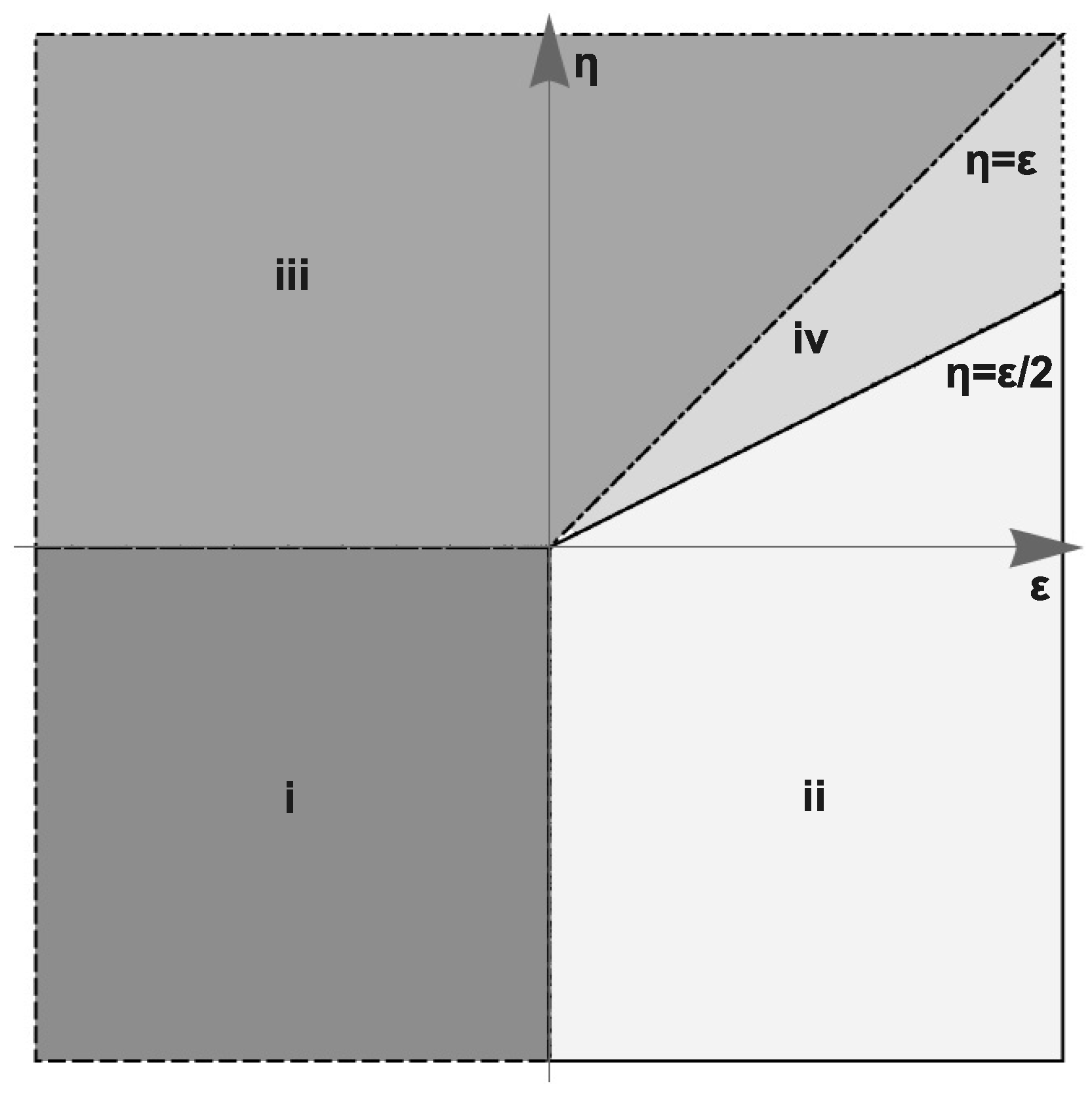
An analysis of the expressions (32) reveals four fixed points:

(i) Gaussian (free) fixed point:

$$g^{*}=0,u^{*}=0;$$

(34)

(ii) Nontrivial fixed point:

$$g^{*}=\frac{2{(\epsilon -\eta )}^2}{\epsilon -2\eta },u^{*}=\frac{\epsilon }{\epsilon -2\eta }.$$

(35)

The point (i) is IR attractive for $\epsilon <0,\eta <0$, while the point (ii) is IR attractive for $\epsilon >0,\eta <\epsilon /2$.

Two more points are found in the following way. In order to explore the limiting case $u\to \infty$ with $g/u$ fixed, we have to pass to new variables: $g^{\prime }\equiv g/u$ and $w\equiv 1/u$. For this case, we obtain

$$\begin{array}{c}\hfill {\beta }_{g^{\prime }}=g^{\prime }\left[\eta -\epsilon +\frac{g^{\prime }}{w+1}\right],{\beta }_w=w\left[\eta +g^{\prime }\frac{w-1}{{(w+1)}^2}\right].\end{array}$$

(36)

Finding the zeros of the $\beta$ functions, we find two additional fixed points:

(iii) Gaussian (free) fixed point:

$$g^{\prime *}=0,w^{*}=0;$$

(37)

(iv) Nontrivial fixed point:

$$g^{\prime *}=\epsilon -\eta ,w^{*}=0.$$

(38)

The point (iii) is IR attractive if $\epsilon >0,\epsilon /2<\eta <\epsilon$, and the point (iv) is IR attractive if $\epsilon <0,\eta >0$ or $\epsilon >0,\eta >\epsilon$.

The general stability pattern of the fixed points in the $\epsilon$–$\eta$ plane is shown in Figure 1.

In the one-loop approximation, the regions of IR stability for all the points are given by sectors that cover the full plane without gaps or overlaps between them.

Some remarks are in order. Clearly, the Gaussian points correspond to cases in which the dynamics of the field $\theta$ are not affected by the statistics of the height field h (only in the leading order of the IR asymptotic behavior!). In these cases, we deal with an ordinary random walk.

The point (iv) corresponds to the limiting case (13) when the field h, in comparison with $\theta$, behaves as if it was $\delta$ correlated in time.

However, we did not find a nontrivial point that would correspond to the frozen limit (14). This follows from the fact that the function ${\beta }_g$ in (32) becomes trivial for $u\to 0$: ${\beta }_g=-\epsilon g$. A similar triviality was observed earlier in models of diffusion in time-independent potential vector fields where it was shown to be exact in all orders of perturbation theory [18,19]. Because those models have a close formal resemblance with the limit (14) of our model and its special case (4) and (6), we believe that in the latter cases ${\beta }_g$ is also trivial exactly.

5. Critical Dimensions and Scaling Behavior

The existence of IR attractive fixed points of the RG equations implies the existence of the scaling behavior of the correlation functions in the IR range.

In dynamical models, the critical dimension of any quantity F (a field or a parameter) is given by the expression (see, e.g., Sections 5.16 and 6.7 in [35] and Section 2.1 in [36])

$${\Delta }_F=d_F^k+{\Delta }_{\omega }{d}_F^{\omega }+{\gamma }_F^{*},{\Delta }_{\omega }=2-{\gamma }_{\nu }^{*}$$

(39)

(with the standard normalization convention that ${\Delta }_{\mathbf{k}}=-{\Delta }_{\mathbf{x}}=1$). Here and below, ${\gamma }^{*}$ denotes the value of the anomalous dimension $\gamma$ at a fixed point.

For the Gaussian points (i) and (iii), one has

$$\begin{array}{c}\hfill {\Delta }_{{\theta }^{\prime }\theta }=d,{\Delta }_{\omega }=2.\end{array}$$

(40)

For the fixed point (ii), one obtains the exact results from the relation (29) and definition (30):

$$\begin{array}{c}\hfill {\Delta }_{{\theta }^{\prime }\theta }=d,{\Delta }_{\omega }=2-\eta .\end{array}$$

(41)

As already mentioned, the point (iv) corresponds to the limit (13), where the propagator ${\langle hh\rangle }_0$ becomes $\delta$-correlated in time. As a result, closed circuits of retarded propagators ${\langle \theta {\theta }^{\prime }\rangle }_0$ appear in almost all diagrams relevant for a renormalization procedure and they therefore vanish. The only exception is the one-loop diagram contributing to ${\mathrm{Z}}_1$. Thus, one has ${\mathrm{Z}}_2=1$ identically, while ${\mathrm{Z}}_1$ is given exactly by the one-loop expression, cf. the discussion of Kraichnan’s rapid-change model of passive scalar advection [38]. Then, one readily derives the exact expressions for the critical dimensions:

$$\begin{array}{c}\hfill {\Delta }_{{\theta }^{\prime }\theta }=d,{\Delta }_{\omega }=2-\epsilon +\eta .\end{array}$$

(42)

As an illustrative application, consider the mean-square distance of a random walker on a rough surface. For such a particle that started moving at $t=0$ from the origin $\mathbf{x}=0$, it is given by

$$R^2\left(t\right)=\int d\mathbf{x}{x}^2\langle \theta (t,\mathbf{x}){\theta }^{\prime }(0,\mathbf{0})\rangle ,$$

(43)

where $t>0$ is a later time and $\mathbf{x}$ is the corresponding current position. Substituting the scaling representation for the linear response function

$$P(t,\mathbf{x})=\langle \theta (t,\mathbf{x}){\theta }^{\prime }(0,\mathbf{0})\rangle \simeq r^{-{\Delta }_{\theta {\theta }^{\prime }}}F\left(t{r}^{-{\Delta }_{\omega }}\right)$$

(44)

gives

$$R^2\left(t\right)\propto t^{(d+2-{\Delta }_{\theta {\theta }^{\prime }})/{\Delta }_{\omega }}.$$

(45)

Taking into account the exact relation ${\Delta }_{{\theta }^{\prime }\theta }=d$, valid for all fixed points (i)-(iv), one arrives at the spreading law

$$R^2\left(t\right)\propto t^{2/{\Delta }_{\omega }},$$

(46)

with the exact expressions ${\Delta }_{\omega }=2$ for the points (i), (iii), ${\Delta }_{\omega }=2-\eta$ for (ii), and ${\Delta }_{\omega }=2-\epsilon +\eta$ for (iv).

6. Conclusions

We studied a model of a random walk of a particle on a rough fluctuating surface described by the Fokker–Planck equation for a particle in a constant gravitational field while the surface was modeled by the (generalized) Edwards–Wilkinson model. The full stochastic problem, (2), (3), (7) and (8), is mapped onto a multiplicatively renormalizable field-theoretic model (16) and (17).

The corresponding RG equations reveal two Gaussian (free) and two nontrivial fixed points, which means that the system exhibits various types of IR scaling behavior (long times and large distances). Although the practical calculation is confined within the leading one-loop approximation, the main critical dimensions are found exactly.

As an illustrative example, we considered the mean-square displacement of a walking particle (in another interpretation, the radius of particles’ cloud). It shows that the particle is not trapped in a finite area but travels all across the system with a spreading law similar to the ordinary random walk but, in general, with different exponents, see (46) and the text below.

As one can see, even a comparatively simple model demonstrates interesting types of IR behavior. Thus, it is interesting to study more involved situations. There are several directions for possible generalizations.

Linear stochastic equations such as (4) and (7) (corresponding to Gaussian statistics for the height field) can be replaced by nonlinear models, such as the KPZ [2] or Pavlik’s [5,8] ones.

Although our expressions (41) and (42) for the critical dimensions are exact, they are derived within perturbation theory based on the assumption that the expansion parameters $\epsilon$ and $\eta$ are small. Then, it is supposed that the one-loop pattern of fixed points is qualitatively correct. However, in some cases, a crossover in the scaling behavior occurs for finite values of parameters analogous to $\epsilon$ and $\eta$ [37,39]. In the field-theoretic approach, this effect can be related to the appearance of composite operators with negative dimensions [37]. This issue requires a special investigation.

On some occasions, the motion of a particle is not an ordinary random walk (1) but is described, e.g., by Lévy flights, see, e.g., [21]. This possibility is supported by the ideas of self-organized criticality that the underlying surface evolves via avalanches [31,32,33,34], while the particle can slide upon the surface. If so, it is natural to replace the Laplace operator in the Fokker–Planck equation (2) with a fractional derivative, $-{\partial }^2\sim k^2\to k^{2-{\eta }^{\prime }}$, with a certain new exponent ${\eta }^{\prime }$.

It is especially interesting to include anisotropy (as a consequence of an overall tilt of the surface). This can be done by describing the field h by the Pastor-Satorras–Rothman model for an eroding landscape [9,10] or the Hwa–Kardar model of a running sandpile [40,41].

This work remains for the future and is partly in progress.

References

- Edwards, S.F.; Wilkinson, D.R. The Surface Statistics of a Granular Aggregate. Proc. R. Soc. 1982, 381, 17–31. [Google Scholar]
- Kardar, M.; Parisi, G.; Zhang, Y.-C. Dynamic scaling of growing interfaces. Phys. Rev. Lett. 1986, 56, 889–892. [Google Scholar] [CrossRef] [PubMed] [Green Version]
- Yan, H.; Kessler, D.A.; Sander, L.M. Roughening phase transition in surface growth. Phys. Rev. Lett. 1990, 64, 926–929. [Google Scholar] [CrossRef] [PubMed]
- Yan, H.; Kessler, D.A.; Sander, L.M. Kinetic Roughening in Surface Growth. MRS Online Proc. Libr. 1992, 278, 237–247. [Google Scholar] [CrossRef]
- Pavlik, S.I. Scaling for a growing phase boundary with nonlinear diffusion. JETP 1994, 79, 303, [Translated from the Russian: ZhETF 1994, 106, 553.]. [Google Scholar]
- Halpin-Healy, T.; Zhang, Y.-C. Kinetic roughening phenomena, stochastic growth, directed polymers and all that. Aspects of multidisciplinary statistical mechanics. Phys. Rep. 1995, 254, 215–414. [Google Scholar] [CrossRef]
- Barabási, A.-L.; Stanley, H.E. Fractal Concepts in Surface Growth; Cambridge University Press: Cambridge, MA, USA, 1995. [Google Scholar]
- Antonov, N.V.; Vasil’ev, A.N. The quantum-field renormalization group in the problem of a growing phase boundary. JETP 1995, 81, 485, [Translated from the Russian: ZhETF 1995, 108, 885.]. [Google Scholar]
- Pastor-Satorras, R.; Rothman, D.H. Stochastic equation for the erosion of inclined topography. Phys. Rev. Lett. 1998, 80, 4349–4352. [Google Scholar] [CrossRef] [Green Version]
- Pastor-Satorras, R.; Rothman, D.H. Scaling of a slope: The erosion of tilted landscapes. J. Stat. Phys. 1998, 93, 477–500. [Google Scholar] [CrossRef]
- Antonov, N.V.; Kakin, P.I. Scaling in erosion of landscapes: Renormalization group analysis of a model with infinitely many couplings. Theor. Math. Phys. 2017, 190, 193–203. [Google Scholar] [CrossRef] [Green Version]
- Duclut, C.; Delamotte, B. Nonuniversality in the erosion of tilted landscapes. Phys. Rev. E 2017, 96, 012149. [Google Scholar] [CrossRef] [Green Version]
- Song, T.; Xia, H. Kinetic roughening and nontrivial scaling in the Kardar–Parisi–Zhang growth with long-range temporal correlations. J. Stat. Mech. 2021, 2021, 073203. [Google Scholar] [CrossRef]
- Marinari, E.; Parisi, G.; Ruelle, D.; Windey, P. Random Walk in a Random Environment and 1/f Noise. Phys. Rev. Lett. 1983, 50, 1223. [Google Scholar] [CrossRef]
- Marinari, E.; Parisi, G.; Ruelle, D.; Windey, P. On the interpretation of 1/f noise. Commun. Math. Phys. 1983, 89, 1–12. [Google Scholar] [CrossRef]
- Fisher, D.S. Random walks in random environments. Phys. Rev. A 1984, 30, 960. [Google Scholar] [CrossRef]
- Fisher, D.S.; Friedan, D.; Qiu, Z.; Shenker, S.J.; Shenker, S.H. Random walks in two-dimensional random environments with constrained drift forces. Phys. Rev. A 1985, 31, 3841–3845. [Google Scholar] [CrossRef]
- Kravtsov, V.E.; Lerner, I.V.; Yudson, V.I. The Einstein relation and exact Gell-Mann-Low function for random walks in media with random drifts. Phys. Lett. A 1986, 119, 203–206. [Google Scholar] [CrossRef]
- Honkonen, J.; Pis’mak, Y.M.; Vasil’ev, A.N. Zero beta function for a model of diffusion in potential random field. J. Phys. A Math. Gen. 1988, 21, L835–L841. [Google Scholar] [CrossRef]
- Bouchaud, J.-P.; Georges, A. Anomalous diffusion in disordered media: Statistical mechanisms, models and physical applications. Phys. Rep. 1990, 195, 127–293. [Google Scholar] [CrossRef]
- Metzler, R.; Klafter, J. The random walk’s guide to anomalous diffusion: A fractional dynamics approach. Phys. Rep. 2000, 339, 1–77. [Google Scholar] [CrossRef]
- Zeitouni, O. Random walks in random environment. In Computational Complexity; Meyers, R., Ed.; Springer: New York, NY, USA, 2012. [Google Scholar]
- Révész, P. Random Walk in Random and Non-Random Environments, 3rd ed.; World Scientific Book: Singapore, 2013. [Google Scholar]
- Haldar, A.; Basu, A. Marching on a rugged landscape: Universality in disordered asymmetric exclusion processes. Phys. Rev. Res. 2020, 2, 043073. [Google Scholar] [CrossRef]
- Hairer, M. Solving the KPZ equation. Ann. Math. 2013, 178, 559–664. [Google Scholar] [CrossRef] [Green Version]
- Hairer, M.; Shen, H. A central limit theorem for the KPZ equation. arXiv 2016, arXiv:1507.01237. [Google Scholar] [CrossRef] [Green Version]
- Hairer, M. Exactly solving the KPZ equation. In Random Growth Models. Proceedings of Symposia in Applied Mathematics; Damron, M., Rassoul-Agha, F., Seppäläinen, T., Damron, M., Rassoul-Agha, F., Seppäläinen, T., Eds.; American Mathematical Society: Providence, RI, USA, 2018; Volume 75, p. 75. [Google Scholar]
- Corwin, I.; Shen, H. Some recent progress in singular stochastic partial differential equations. Bull. Am. Math. Soc. 2020, 57, 409–454. [Google Scholar] [CrossRef] [Green Version]
- Barraquand, G.; Corwin, I. Stationary measures for the log-gamma polymer and KPZ equation in half-space. arXiv 2022, arXiv:2203.11037. [Google Scholar]
- Falkovich, G.; Gawȩdzki, K.; Vergassola, M. Particles and fields in fluid turbulence. Rev. Mod. Phys. 2001, 73, 913–975. [Google Scholar] [CrossRef]
- Pruessner, G. Self-Organized Criticality: Theory, Models and Characterisation; Cambridge University Press: Cambridge, MA, USA, 2012. [Google Scholar]
- Bak, P.; Tang, C.; Wiesenfeld, K. Self-organized criticality: An explanation of the 1/f noise. Phys. Rev. Lett. 1987, 59, 381–384. [Google Scholar] [CrossRef]
- Bak, P.; Tang, C.; Wiesenfeld, K. Self-organized criticality. Phys. Rev. A 1988, 38, 364–374. [Google Scholar] [CrossRef]
- Maslov, S.; Tang, C.; Zhang, Y.-C. 1/f Noise in Bak-Tang-Wiesenfeld Models on Narrow Stripes. Phys. Rev. Lett. 1999, 83, 2449–2452. [Google Scholar] [CrossRef] [Green Version]
- Vasiliev, A.N. The Field Theoretic Renormalization Group in Critical Behaviour Theory and Stochastic Dynamics; Chapman & Hall/CRC: Boca Raton, FL, USA, 2004; [Translated from the Russian: St Petersburg Institute of Nuclear Physics: Gatchina, Russia, 1999; ISBN 5-86763-122-2. [Google Scholar]
- Adzhemyan, L.T.; Antonov, N.V.; Vasil’ev, A.N. The Field Theoretic Renormalization Group in Fully Developed Turbulence; Gordon & Breach: London, UK, 1999. [Google Scholar]
- Antonov, N.V. Anomalous scaling regimes of a passive scalar advected by the synthetic velocity field. Phys. Rev. E 1999, 60, 6691–6707. [Google Scholar] [CrossRef] [Green Version]
- Adzhemyan, L.T.; Antonov, N.V.; Vasil’ev, A.N. Renormalization group, operator product expansion, and anomalous scaling in a model of advected passive scalar. Phys. Rev. E 1998, 58, 1823–1835. [Google Scholar] [CrossRef] [Green Version]
- Avellaneda, M.; Majda, A. Mathematical models with exact renormalization for turbulent transport II: Non-Gaussian statistics, fractal interfaces, and the sweeping effect. Commun. Math. Phys. 1992, 146, 139–204. [Google Scholar] [CrossRef]
- Hwa, T.; Kardar, M. Dissipative transport in open systems: An investigation of self-organized criticality. Phys. Rev. Lett. 1989, 62, 1813–1816. [Google Scholar] [CrossRef]
- Hwa, T.; Kardar, M. Avalanches, hydrodynamics and great events in models of sandpiles. Phys. Rev. A 1992, 45, 7002–7023. [Google Scholar] [CrossRef]
Figure 1.
Regions of stability of the fixed points (i)–(iv).
Disclaimer/Publisher’s Note: The statements, opinions and data contained in all publications are solely those of the individual author(s) and contributor(s) and not of MDPI and/or the editor(s). MDPI and/or the editor(s) disclaim responsibility for any injury to people or property resulting from any ideas, methods, instructions or products referred to in the content. |
© 2023 by the authors. Licensee MDPI, Basel, Switzerland. This article is an open access article distributed under the terms and conditions of the Creative Commons Attribution (CC BY) license (https://creativecommons.org/licenses/by/4.0/).
Share and Cite
MDPI and ACS Style
Antonov, N.V.; Gulitskiy, N.M.; Kakin, P.I.; Kerbitskiy, D.A. Random Walk on a Rough Surface: Renormalization Group Analysis of a Simple Model. Universe 2023, 9, 139. https://doi.org/10.3390/universe9030139
AMA Style
Antonov NV, Gulitskiy NM, Kakin PI, Kerbitskiy DA. Random Walk on a Rough Surface: Renormalization Group Analysis of a Simple Model. Universe. 2023; 9(3):139. https://doi.org/10.3390/universe9030139
Chicago/Turabian StyleAntonov, Nikolay V., Nikolay M. Gulitskiy, Polina I. Kakin, and Dmitriy A. Kerbitskiy. 2023. "Random Walk on a Rough Surface: Renormalization Group Analysis of a Simple Model" Universe 9, no. 3: 139. https://doi.org/10.3390/universe9030139
Note that from the first issue of 2016, this journal uses article numbers instead of page numbers. See further details here.