Past, Present, and Future of Face Recognition: A Review


Abstract
:1. Introduction
- Natural character: The face is a very realistic biometric feature used by humans in the individual’s recognition, making it possibly the most related biometric feature for authentication and identification purposes [4]. For example, in access control, it is simple for administrators to monitor and evaluate approved persons after authentication, using their facial characteristics. The support of ordinary employers (e.g., administrators) may boost the efficiency and applicability of recognition systems. On the other hand, identifying fingerprints or iris requires an expert with professional competencies to provide accurate confirmation.
- Nonintrusive: In contrast to fingerprint or iris images, facial images can quickly be obtained without physical contact; people feel more relaxed when using the face as a biometric identifier. Besides, a face recognition device can collect data in a friendly manner that people commonly accept [5].
- Less cooperation: Face recognition requires less assistance from the user compared with iris or fingerprint. For some limited applications such as surveillance, a face recognition device may recognize an individual without active subject involvement [5].
- We provide an updated review of automated face recognition systems: the history, present, and future challenges.
- We present 23 well-known face recognition datasets in addition to their assessment protocols.
- We have reviewed and summarized nearly 180 scientific publications on facial recognition and its material problems of data acquisition and pre-processing from 1990 to 2020. These publications have been classified according to various approaches: holistic, geometric, local texture, and deep learning for 2D and 3D facial recognition. We pay particular attention to the methods based deep-learning, which are currently considered state-of-the-art in 2D face recognition.
- We analyze and compare several in-depth learning methods according to the architecture implemented and their performance assessment metrics.
- We study the performance of deep learning methods under the most commonly used data set: (i) Labeled Face in the Wild (LFW) data set [10] for 2D face recognition, (ii) Bosphorus and BU-3DFE for 3D face recognition.
- We discuss some new directions and future challenges for facial recognition technology by paying particular attention to the aspect of 3D recognition.
2. Face Recognition History
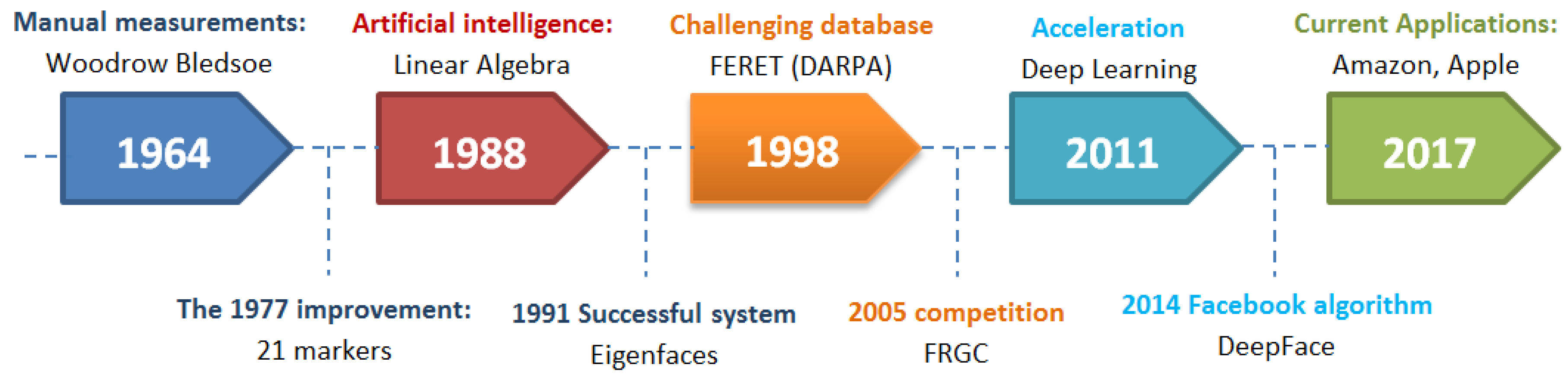
- 1964: The American researchers Bledsoe et al. [11] studied facial recognition computer programming. They imagine a semi-automatic method, where operators are asked to enter twenty computer measures, such as the size of the mouth or the eyes.
- 1977: The system was improved by adding 21 additional markers (e.g., lip width, hair color).
- 1988: Artificial intelligence was introduced to develop previously used theoretical tools, which showed many weaknesses. Mathematics (“linear algebra”) was used to interpret images differently and find a way to simplify and manipulate them independent of human markers.
- 1991: Alex Pentland and Matthew Turk of the Massachusetts Institute of Technology (MIT) presented the first successful example of facial recognition technology, Eigenfaces [12], which uses the statistical Principal component analysis (PCA) method.
- 1998: To encourage industry and the academy to move forward on this topic, the Defense Advanced Research Projects Agency (DARPA) developed the Face recognition technology (FERET) [13] program, which provided to the world a sizable, challenging database composed of 2400 images for 850 persons.
- 2005: The Face Recognition Grand Challenge (FRGC) [14] competition was launched to encourage and develop face recognition technology designed to support existent facial recognition initiatives.
- 2011: Everything accelerates due to deep learning, a machine learning method based on artificial neural networks [9]. The computer selects the points to be compared: it learns better when it supplies more images.
- 2014: Facebook knows how to recognize faces due to its internal algorithm, Deepface [15]. The social network claims that its method approaches the performance of the human eye near to 97%.
- In its new updates, Apple introduced a facial recognition application where its implementation has extended to retail and banking.
- Mastercard developed the Selfie Pay, a facial recognition framework for online transactions.
- From 2019, people in China who want to buy a new phone will now consent to have their faces checked by the operator.
- Chinese police used a smart monitoring system based on live facial recognition; using this system, they arrested, in 2018, a suspect of “economic crime” at a concert where his face, listed in a national database, was identified in a crowd of 50,000 persons.
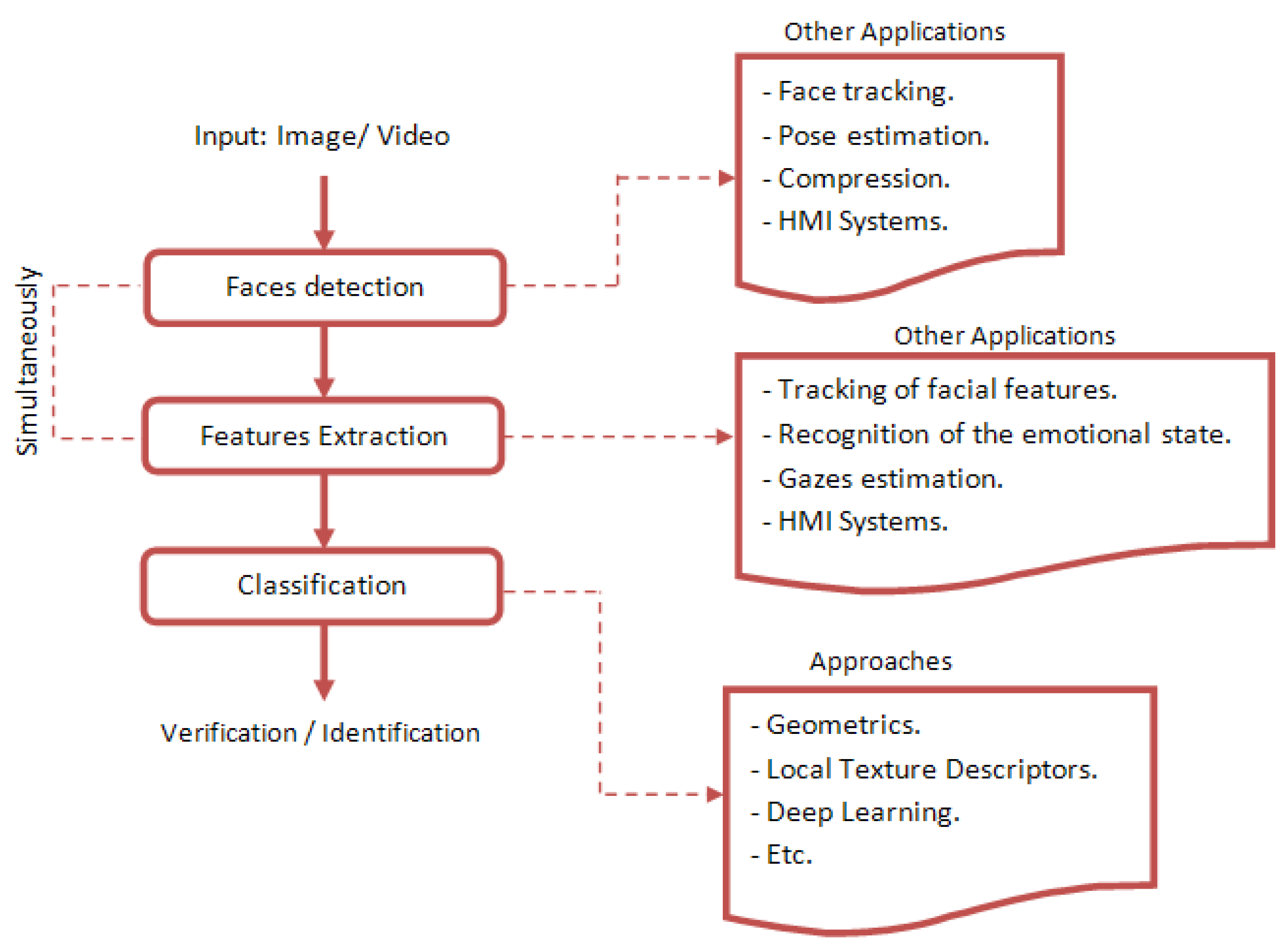
3. Face Recognition Systems
3.1. Main Steps in Face Recognition Systems
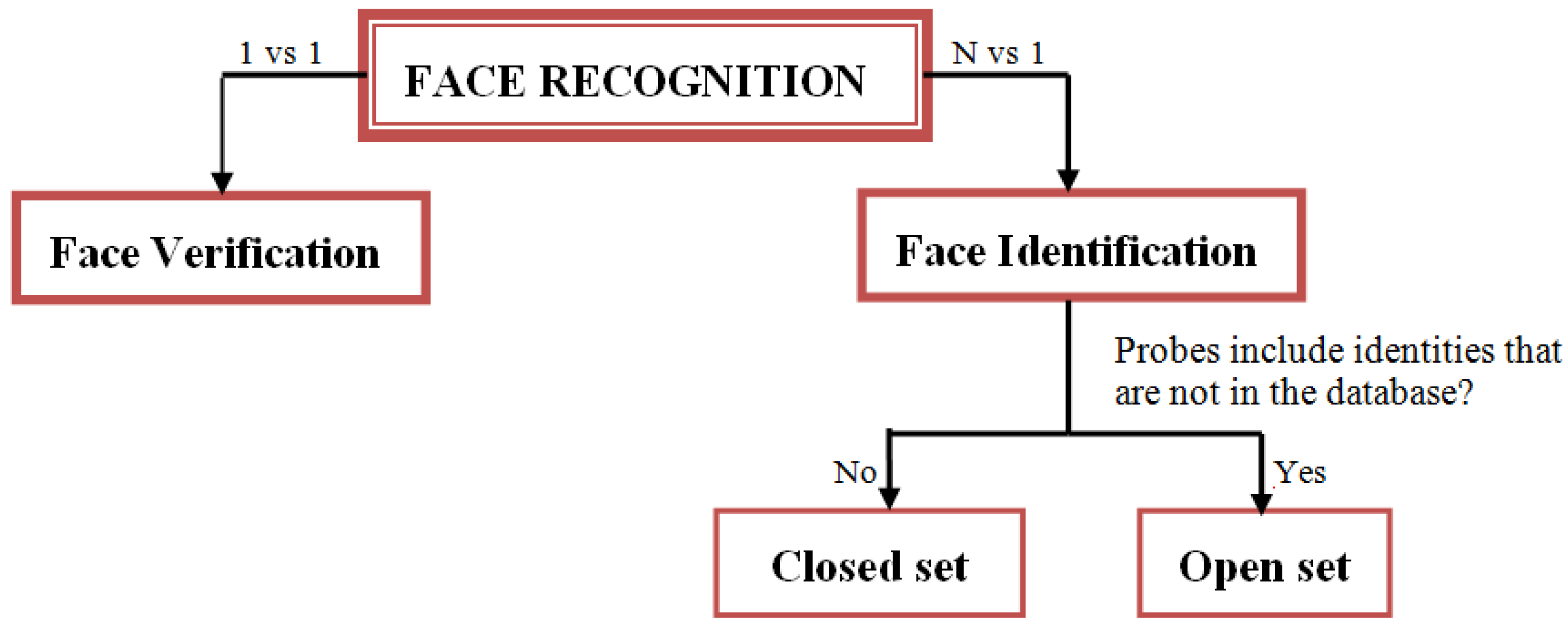
3.2. Assessment Protocols in Face Recognition
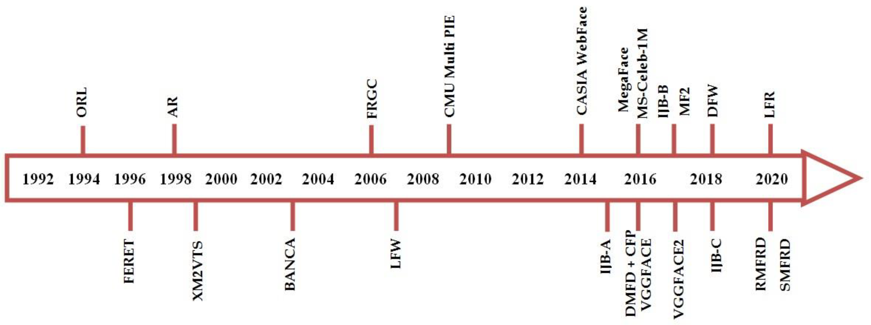
4. Available Datasets and Protocols for 2D Face Recognition
4.1. ORL Dataset
4.2. FERET Dataset
4.3. AR Dataset
4.4. XM2VTS Database
4.5. BANCA Dataset
4.6. FRGC Dataset
- In experimental protocol 1, two controlled still images of an individual are used as one for a gallery, and the other for a probe.
- In Exp 2, the four controlled images of a person are distributed among the gallery and probe.
- In Exp 4, a single controlled still image presents the gallery, and a single uncontrolled still image presents the probe.
- Exps 3, 5, and 6 are designed for 3D images.
4.7. LFW Database
4.8. CMU Multi PIE Dataset
4.9. CASIA-WebFace Dataset
4.10. IARPA Janus Benchmark-A
4.11. MegaFace Database
4.12. CFP Dataset
4.13. Ms-Celeb-M1 Benchmark
4.14. DMFD Database
4.15. VGGFACE Database
4.16. VGGFACE2 Database
4.17. IARPA Janus Benchmark-B
4.18. MF2 Dataset
4.19. DFW Dataset
- Impersonation protocol used only to evaluate the performance of impersonation techniques.
- Obfuscation protocol used in the cases of disguises.
- Overall performance protocol that is used to evaluate any algorithm on the complete dataset.
4.20. IARPA Janus Benchmark-C
4.21. LFR Dataset
4.22. RMFRD and SMFRD: Masqued Face Recognition Dataset
- Masked face detection dataset (MFDD): it can be utilized to train a masked face detection model with precision.
- Real-world masked face recognition dataset (RMFRD): it contains 5000 images of 525 persons wearing masks, and 90,000 pictures of the same 525 individuals without masks collected from the Internet (Figure 17).
- Simulated masked face recognition dataset (SMFRD): in the meantime, the proposers utilized alternative means to place masks on the standard large-scale facial datasets, such as LFW [10] and CASIA WebFace [30] datasets, expanding thus the volume and variety of the masked facial recognition dataset. The SMFRD dataset covers 500,000 facial images of 10,000 persons, and it can be employed in practice alongside their original unmasked counterparts (Figure 18).
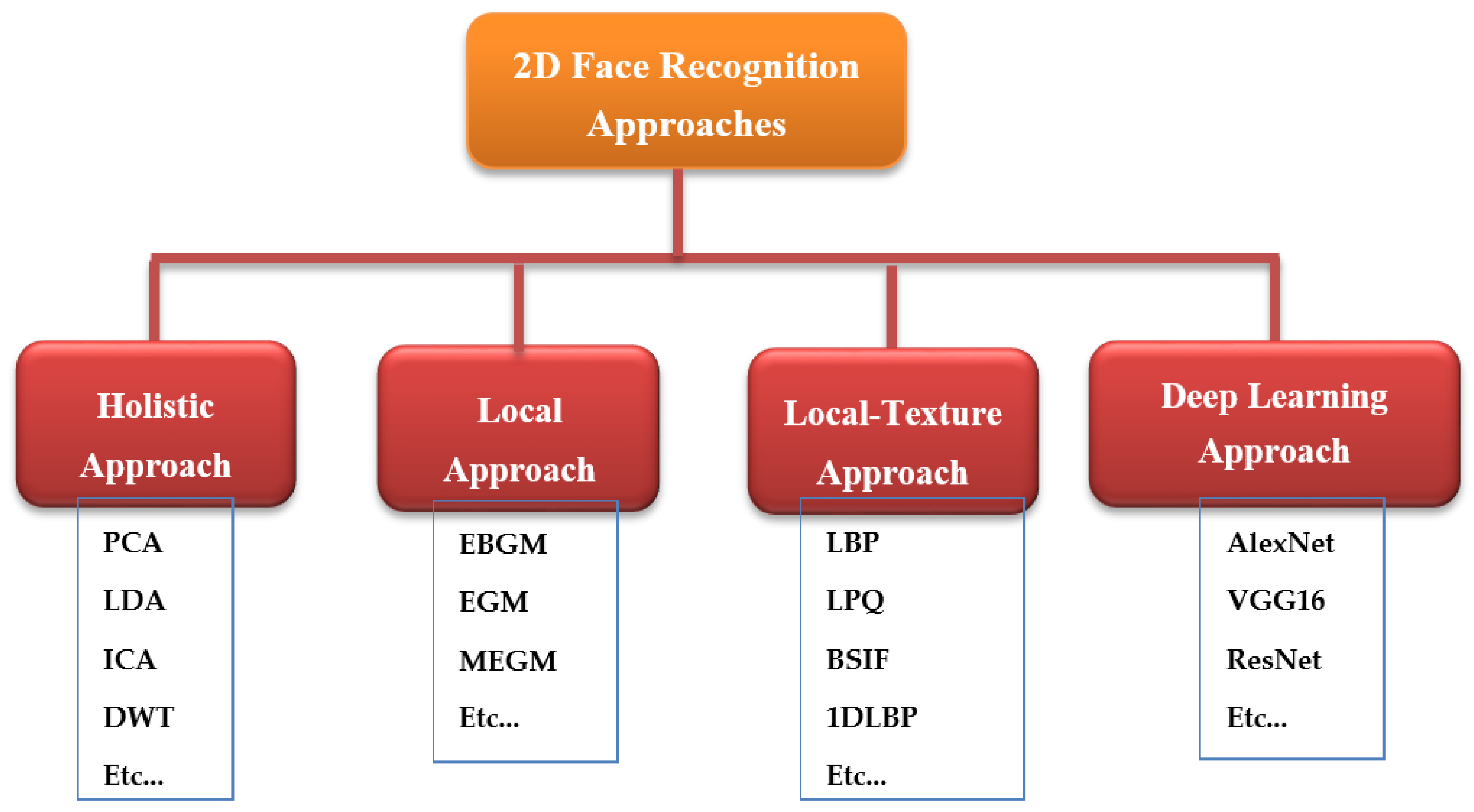
5. Two-Dimensional Face Recognition Approaches
5.1. Holistic Methods
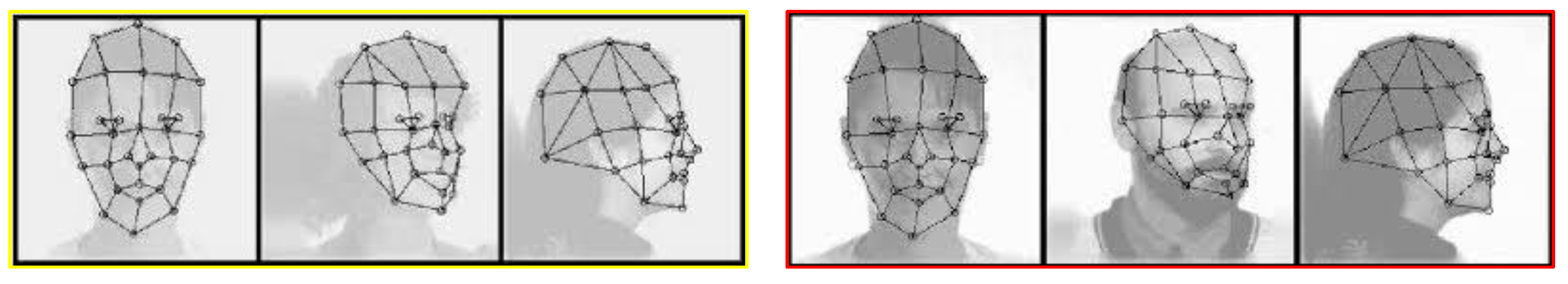
5.2. Geometric Approach
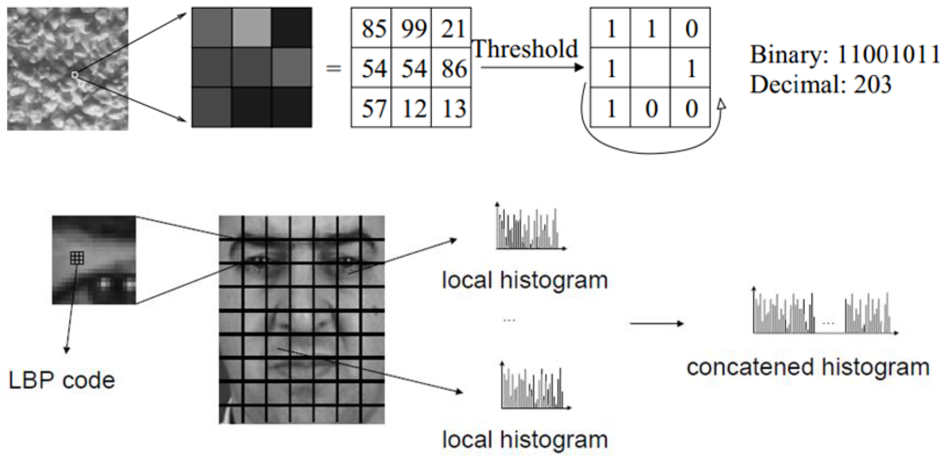
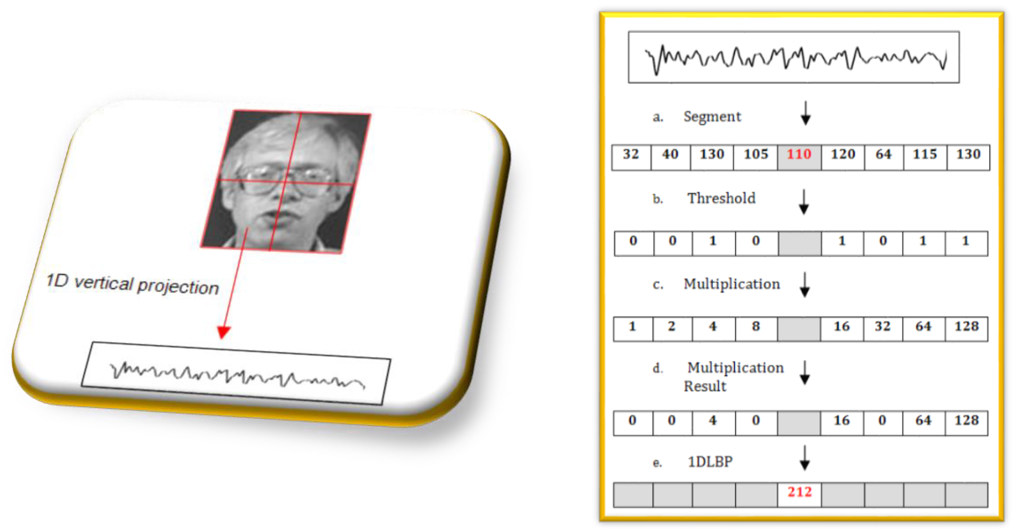
5.3. Local-Texture Approach
5.4. Deep Learning Approach
5.4.1. Introduction to Deep Learning
- Supervised or discriminative (convolutional neural network (CNN));
5.4.2. Convolutional Neural Networks (CNNs)
- Convolutional layer: This is the CNN’s core building block that aims at extracting features from the input data. Each layer uses a convolution operation to obtain a feature map. After that, the activation or feature maps are fed to the next layer as input data [9].
- Rectified linear unit (ReLU) Layer: This is a non-linear operation, involving units that use the rectifier.
- Fully connected layer (FC): The high-level reasoning in the neural network is done via fully connected layers after applying various convolutional layers and max-pooling layers [107].
5.4.3. Popular CNN Architectures
LeNet
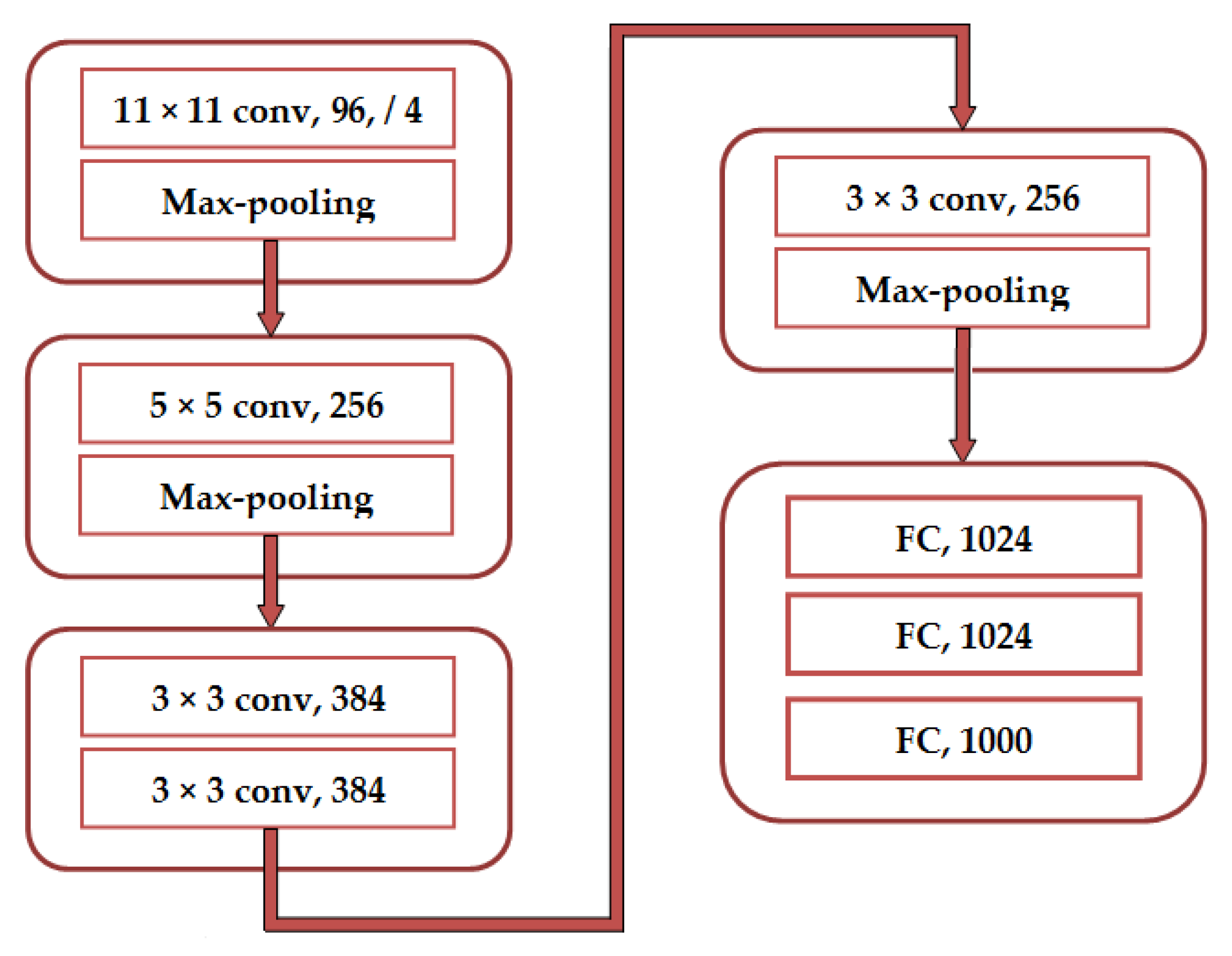
AlexNet
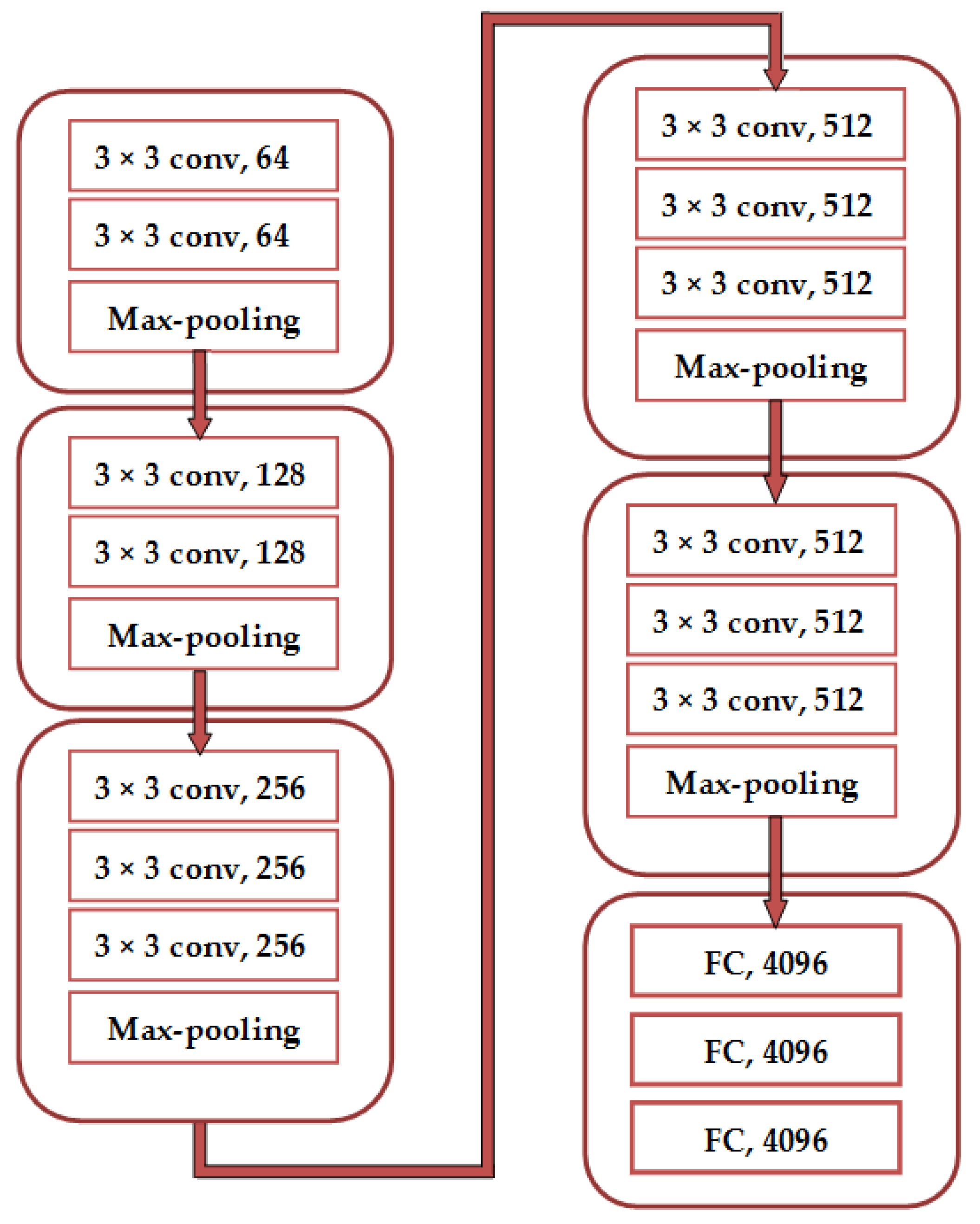
VGGNet
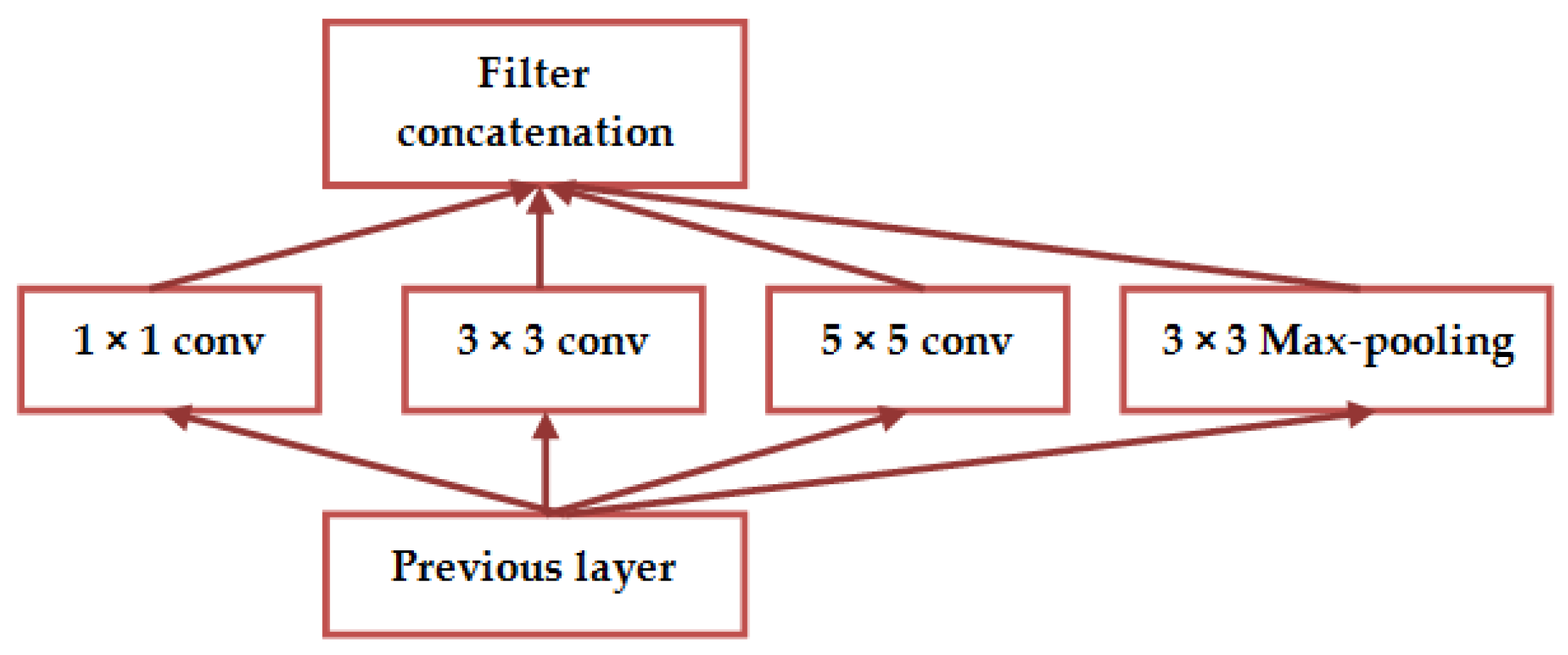
GoogleNet
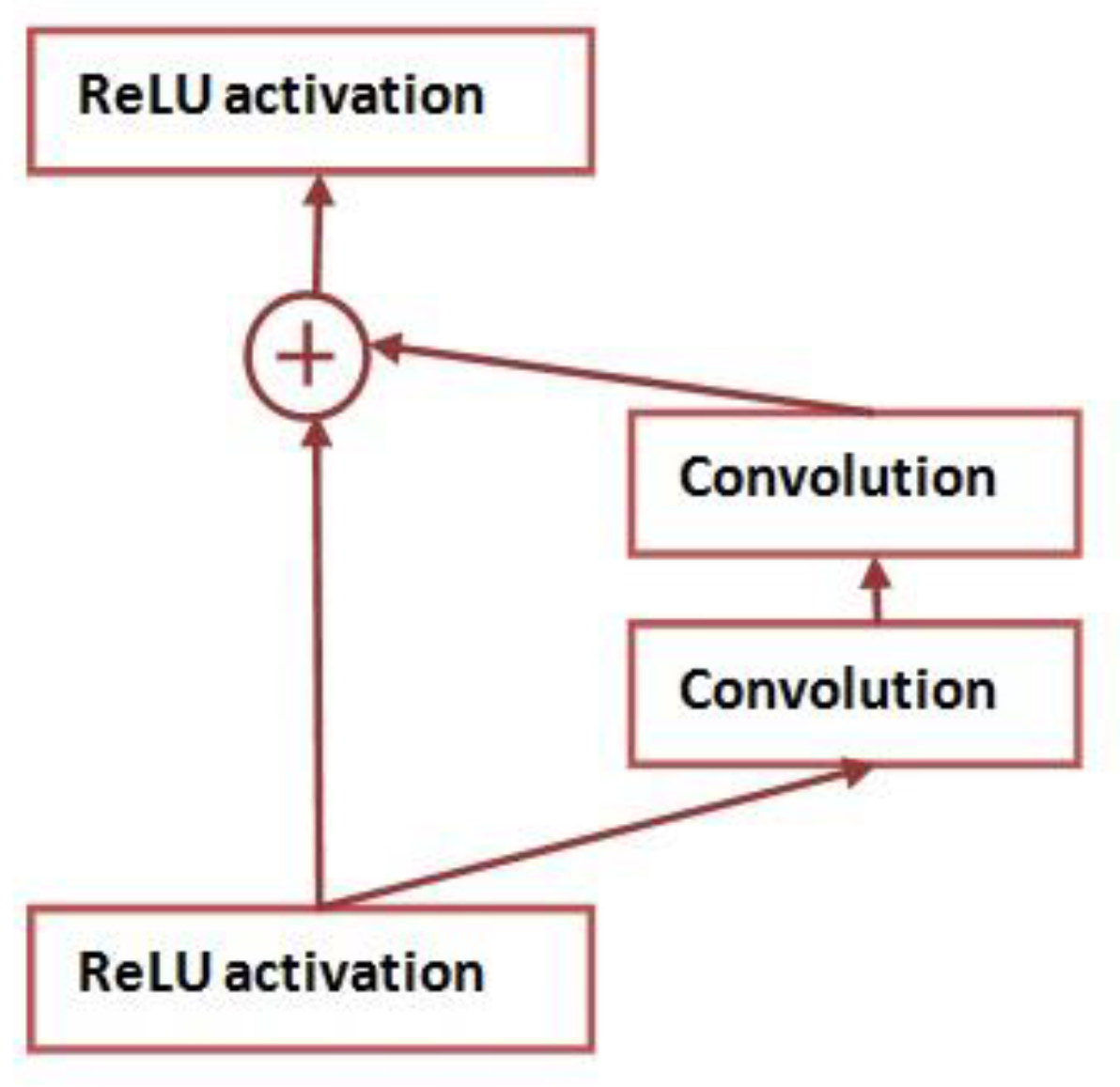
ResNet
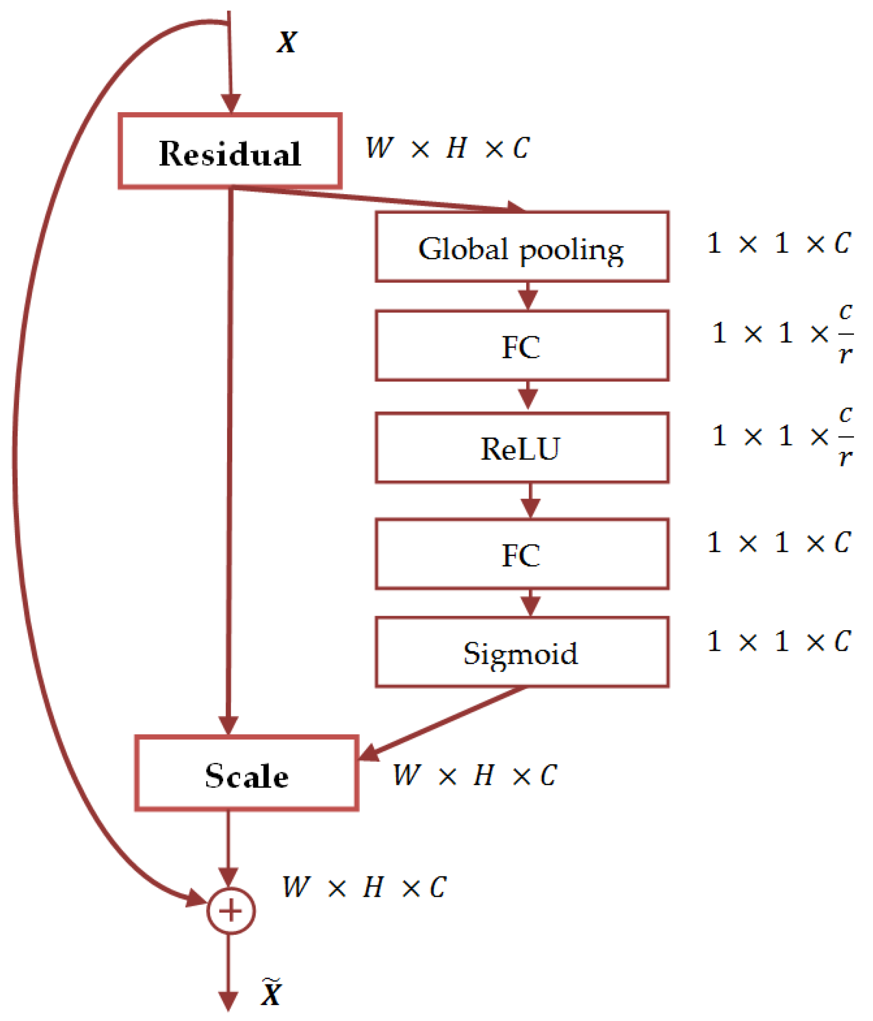
SENet
5.4.4. Deep CNN-Based Methods for Face Recognition.
Investigations Based on AlexNet Architecture
Investigations Based on VGGNet Architecture
Investigations Based on GoogleNet Architecture
Investigations Based on LeNet Architecture
Investigations Based on ResNet Architecture
6. Three-Dimensional Face Recognition
6.1. Factual Background and Acquisition Systems
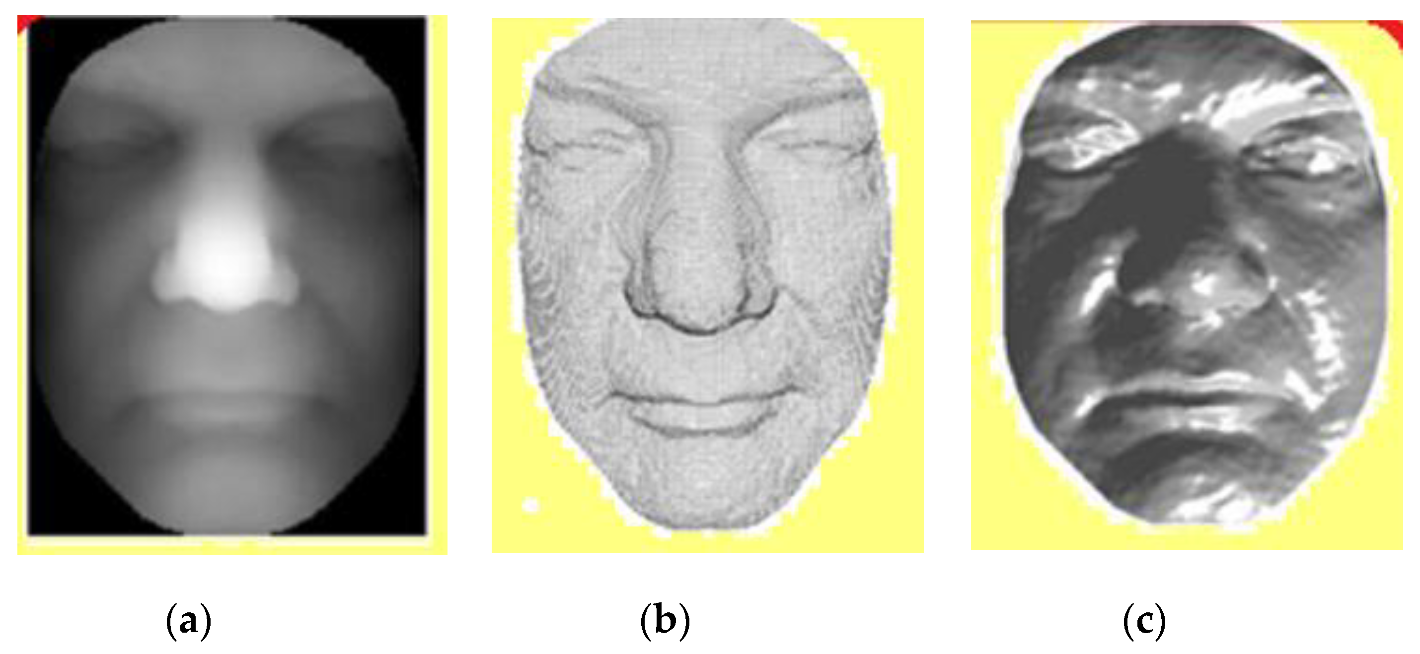
6.1.1. Introduction to 3D Face Recognition
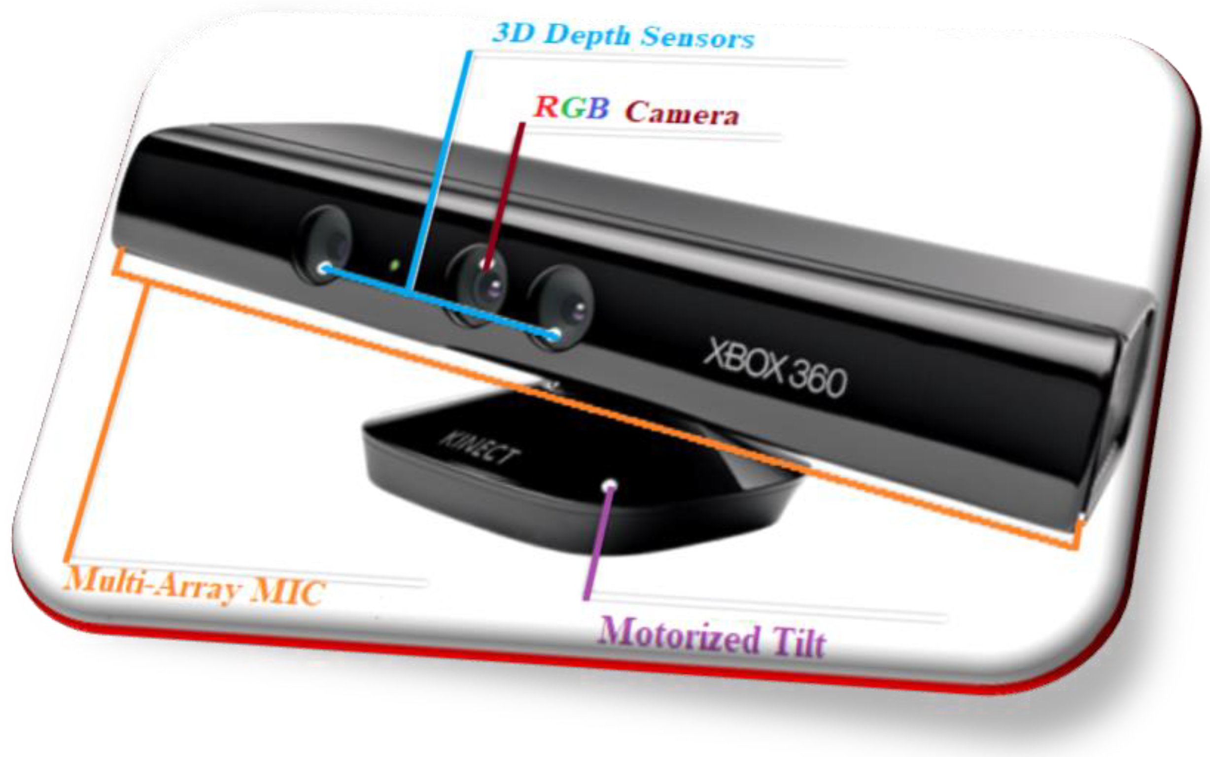
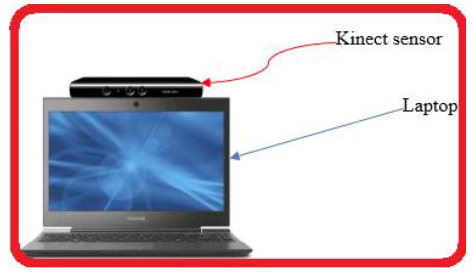
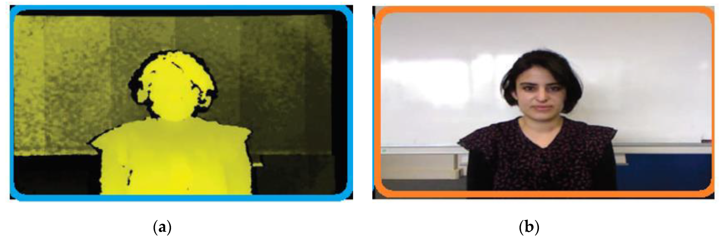
6.1.2. Microsoft Kinect Technology
6.2. Methods and Datasets
6.2.1. Challenges of 3D Facial Recognition
6.2.2. Traditional Methods of Machine Learning
- Traditional methods of machine learning
- Deep learning-based methods.
6.2.3. Deep Learning-Based Methods
6.2.4. Three-Dimensional Face Recognition Databases
7. Open Challenges
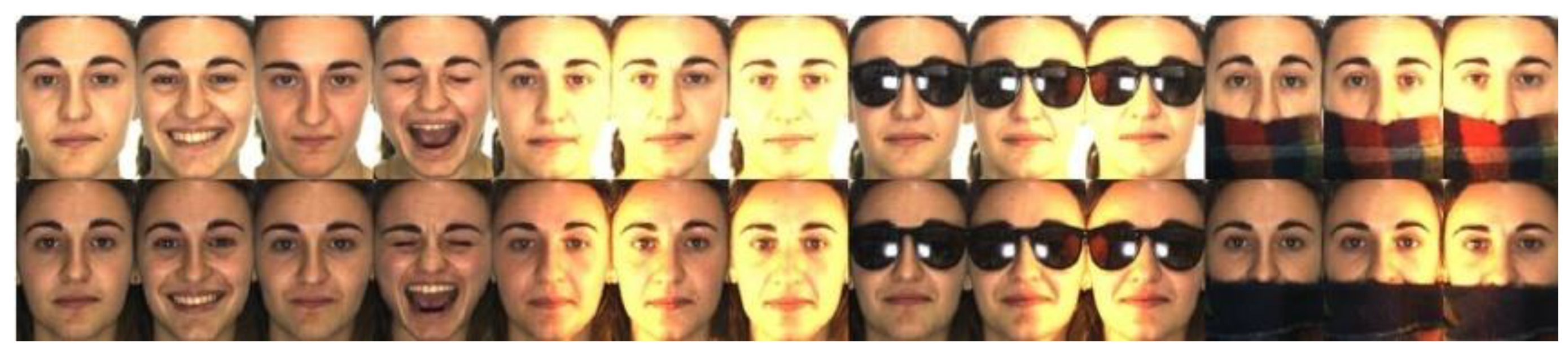
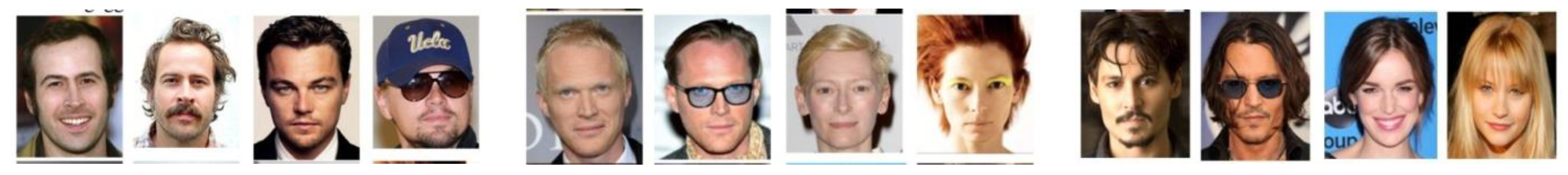
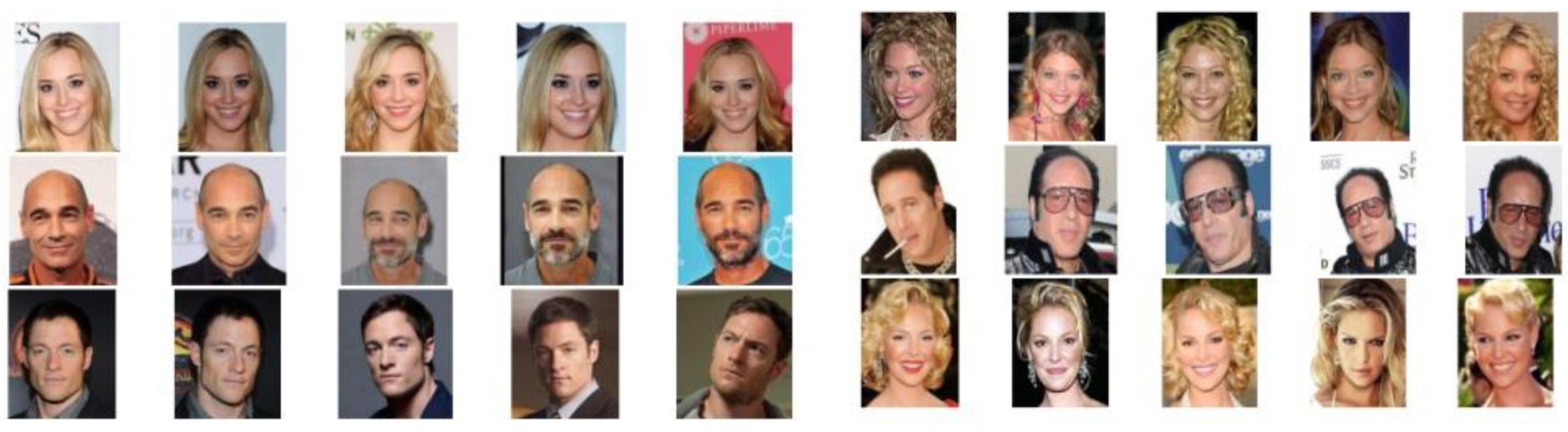
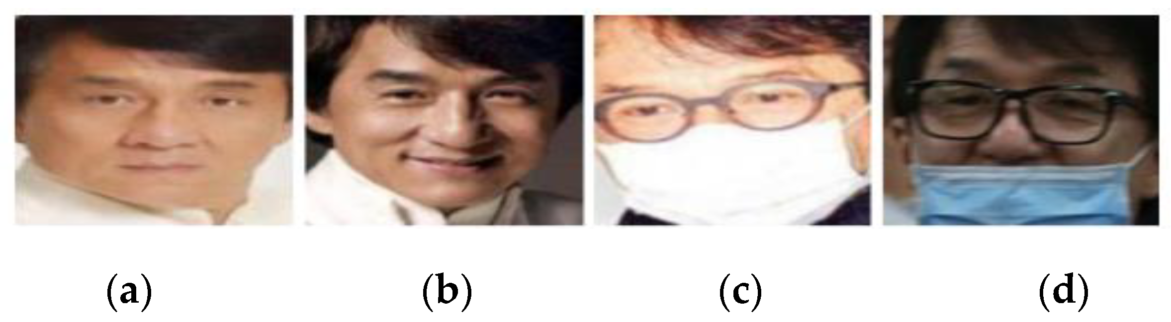
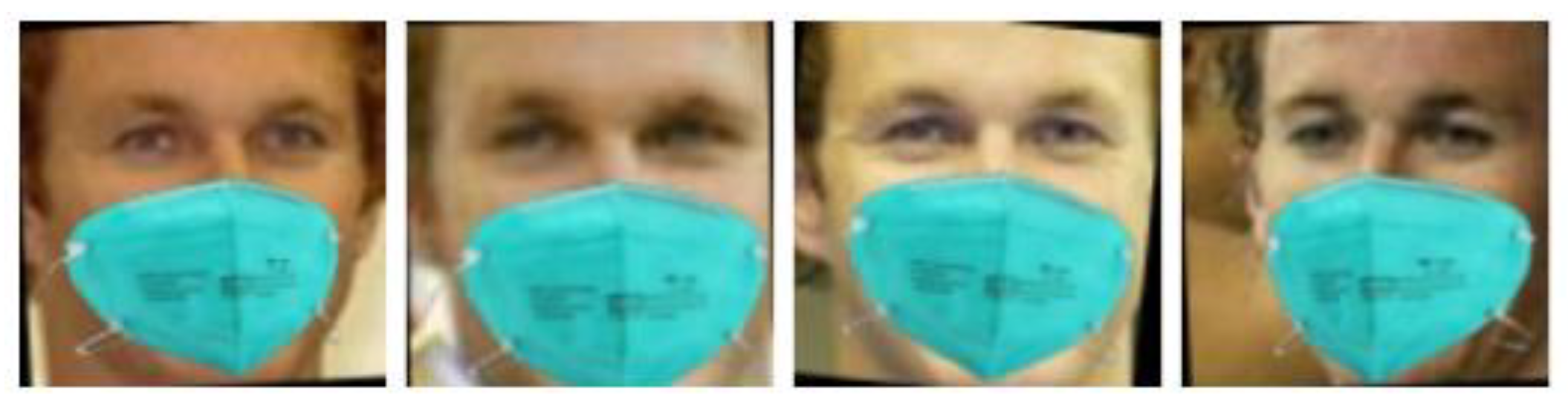
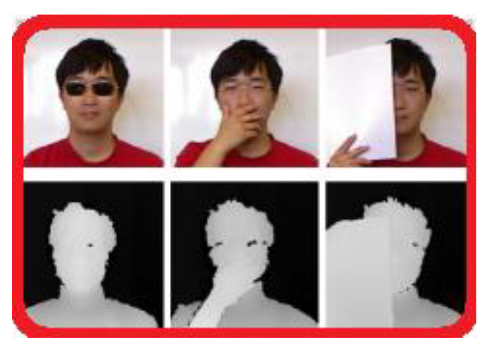
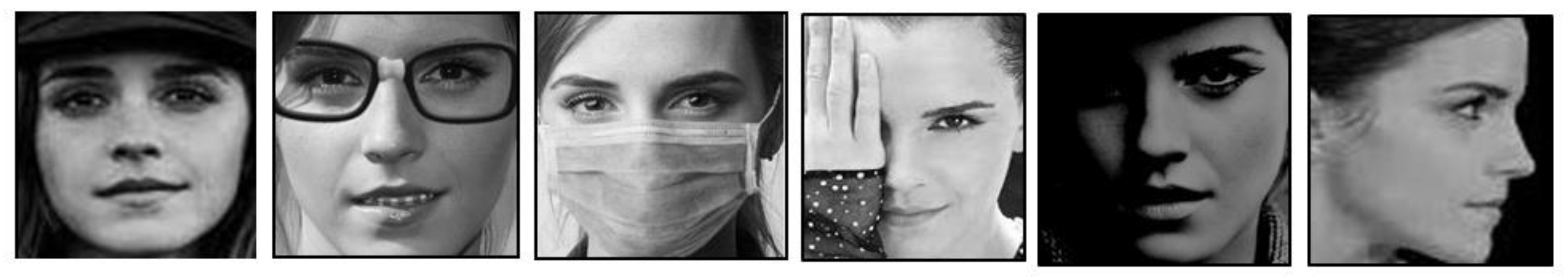
7.1. Face Recognition and Occlusion
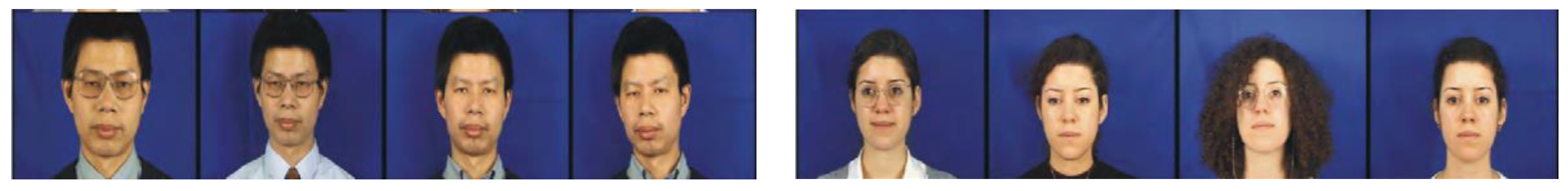
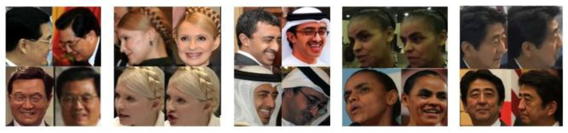
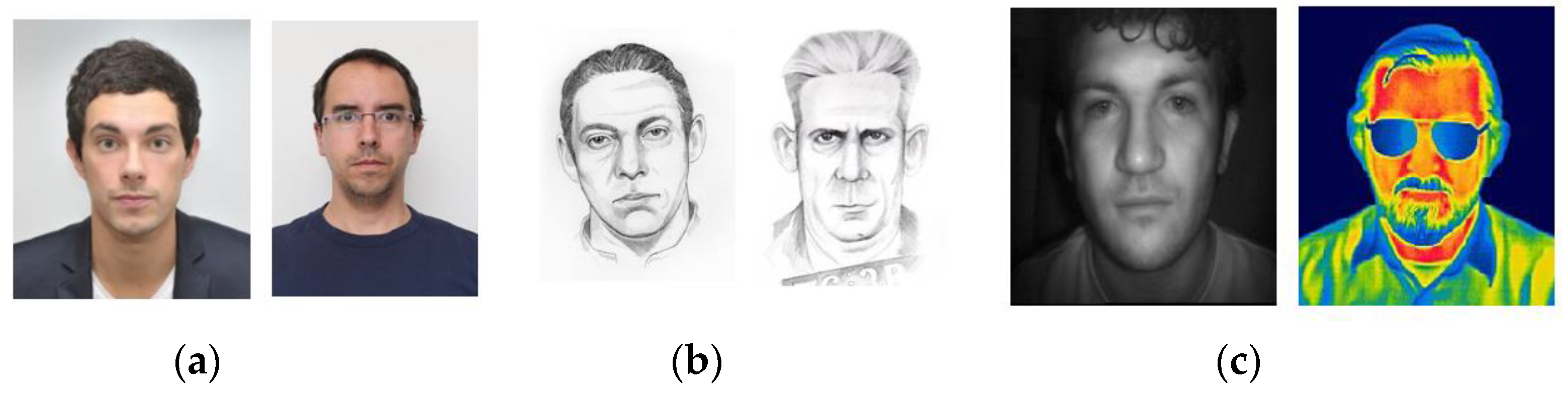
7.2. Hetegerenous Face Recognition
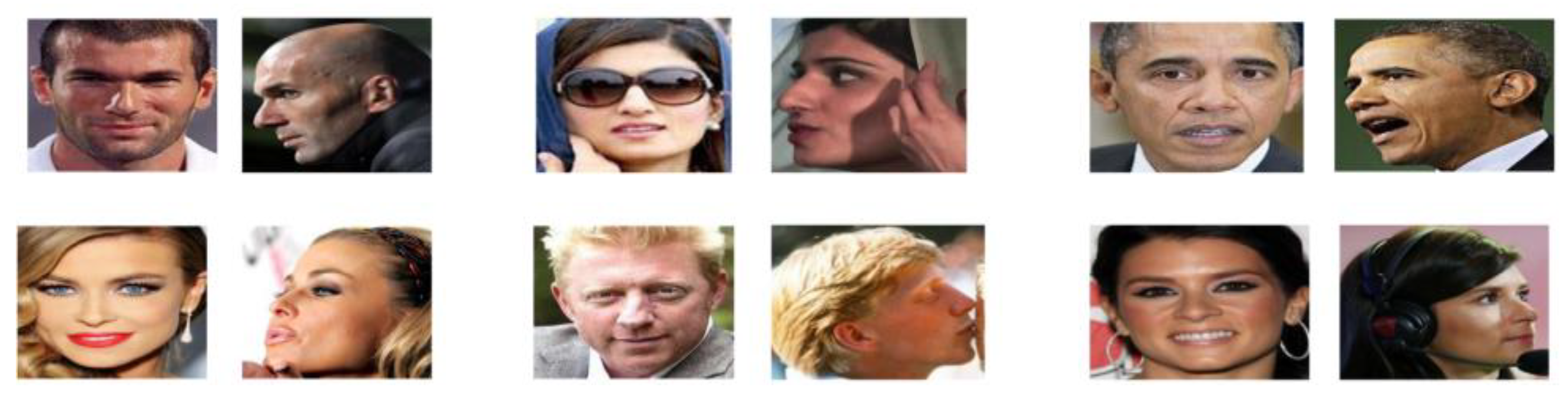
7.3. Face Recognition and Ageing
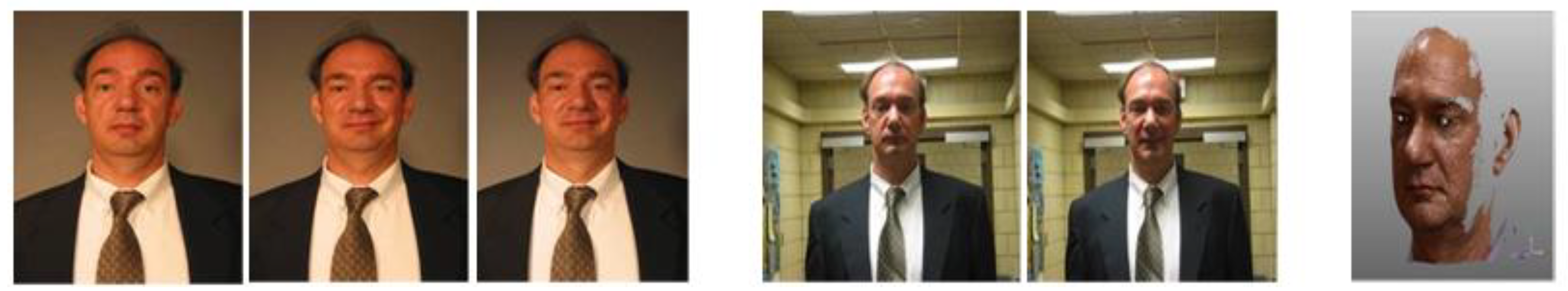
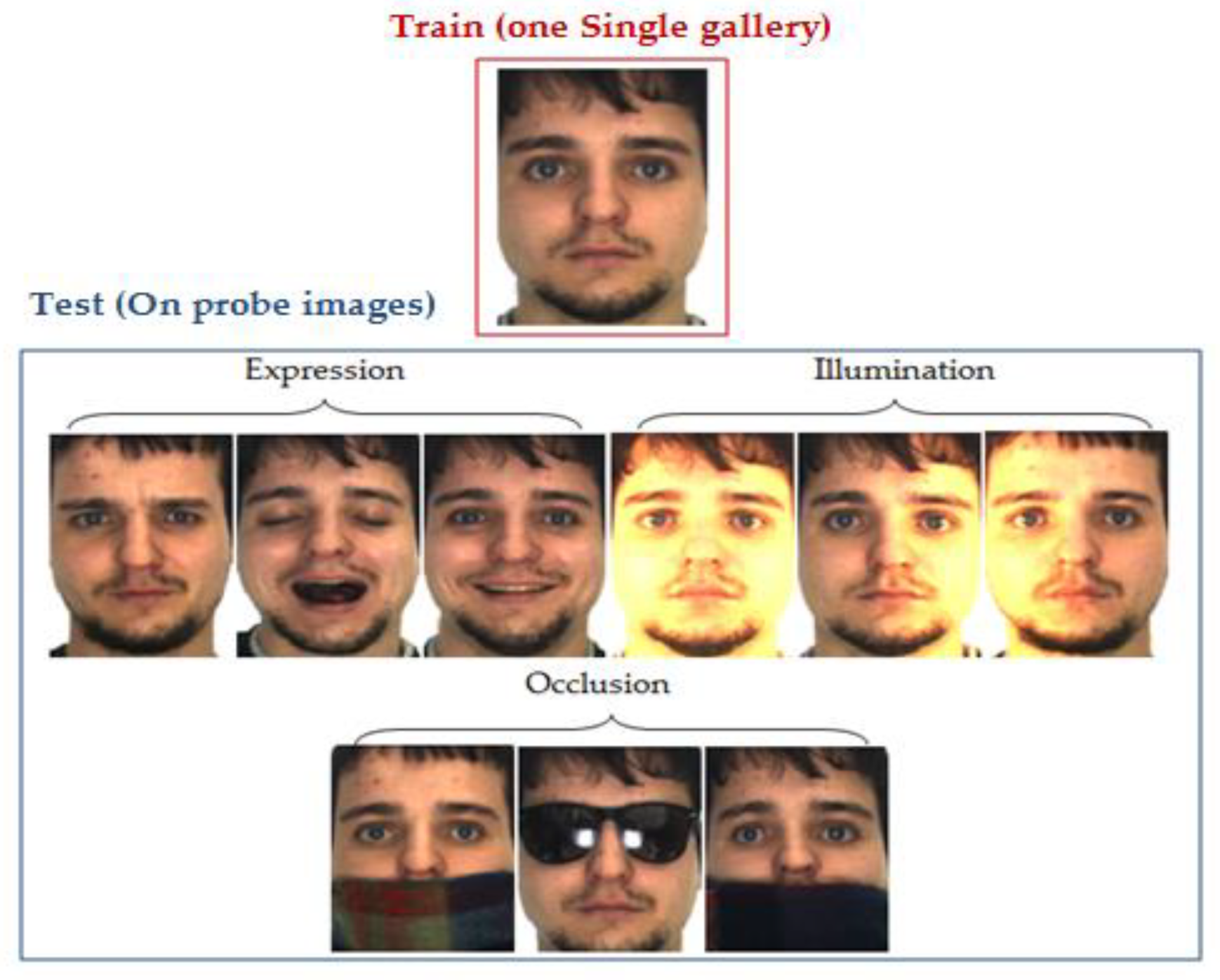
7.4. Single Sample Face Recognition
- In real-world applications (e.g., passports, immigration systems), only one model of each individual is registered in the database and accessible for the recognition task [174].
- Pattern recognition systems require vast training data to ensure the generalization of the learning systems.
- Deep learning-based approach is considered a powerful technique in face recognition. Nonetheless, they need a significant amount of training data to perform well [9].
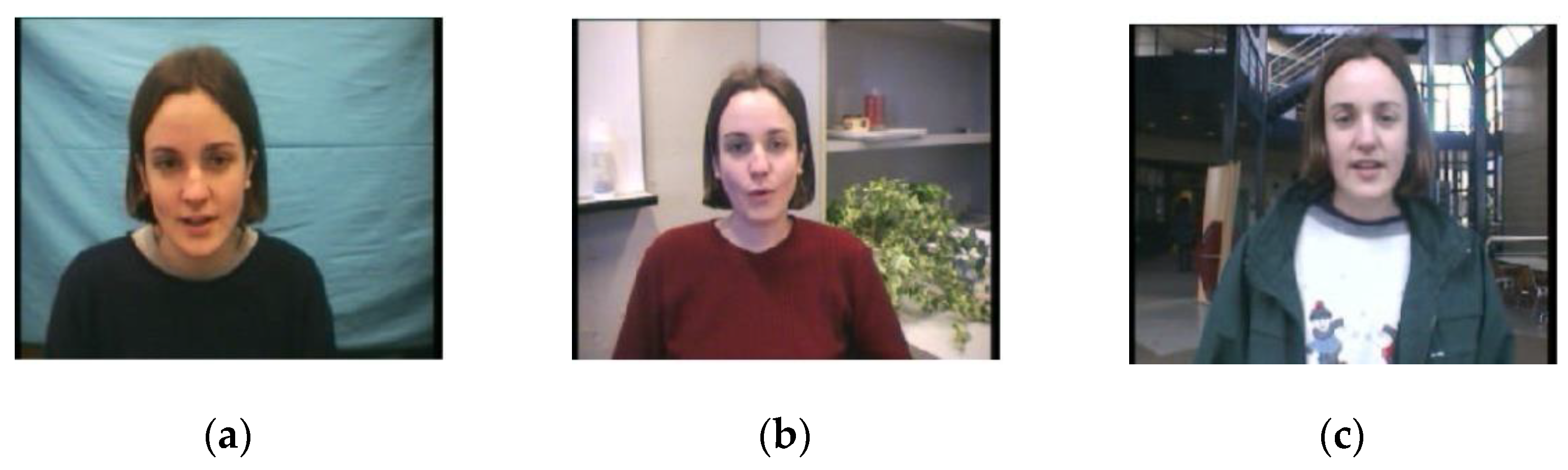
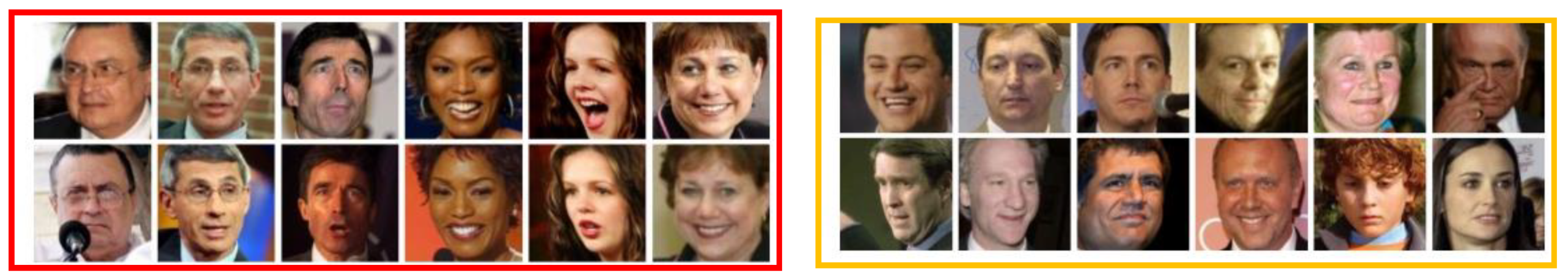
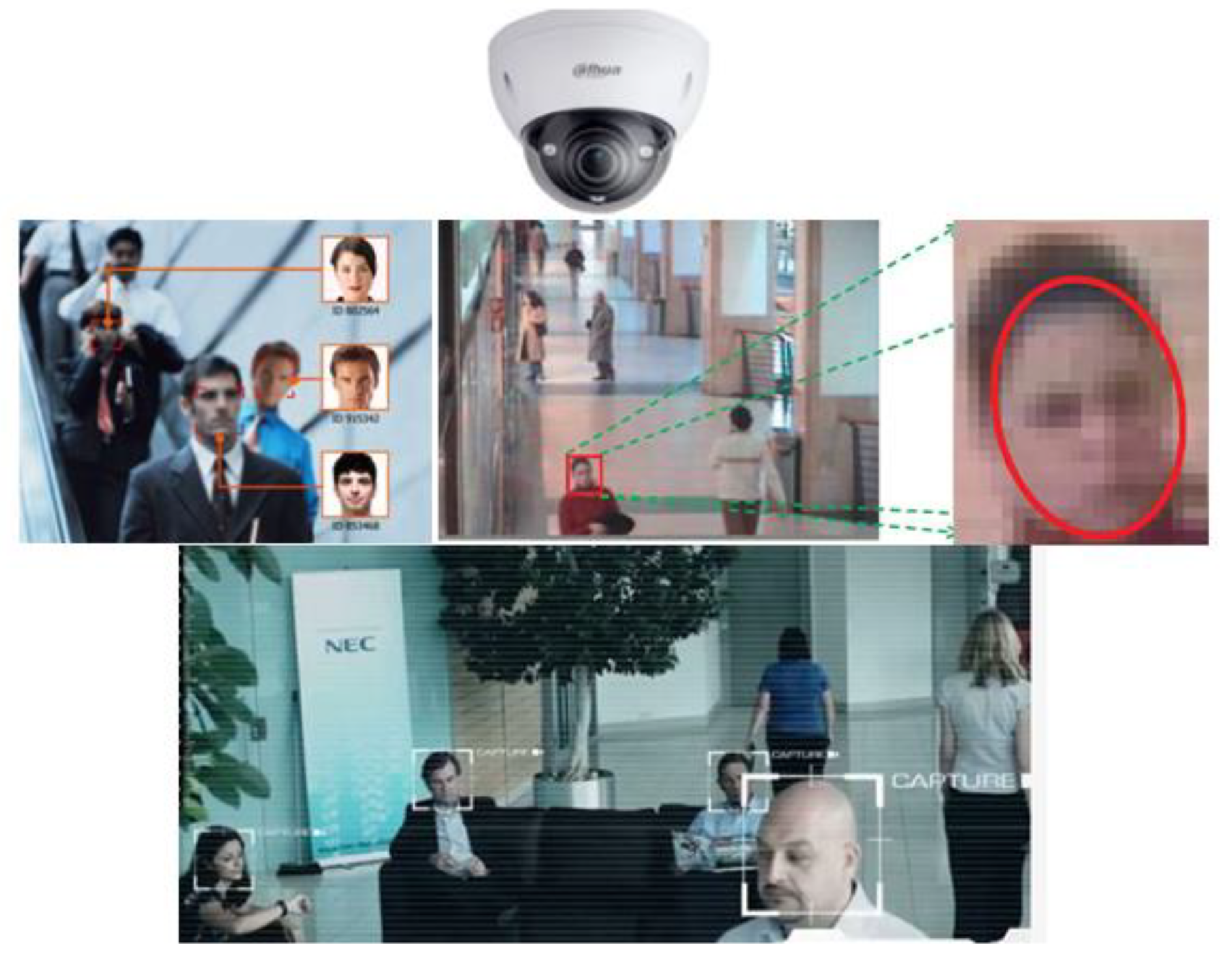
7.5. Face Recognition in Video Surveillance
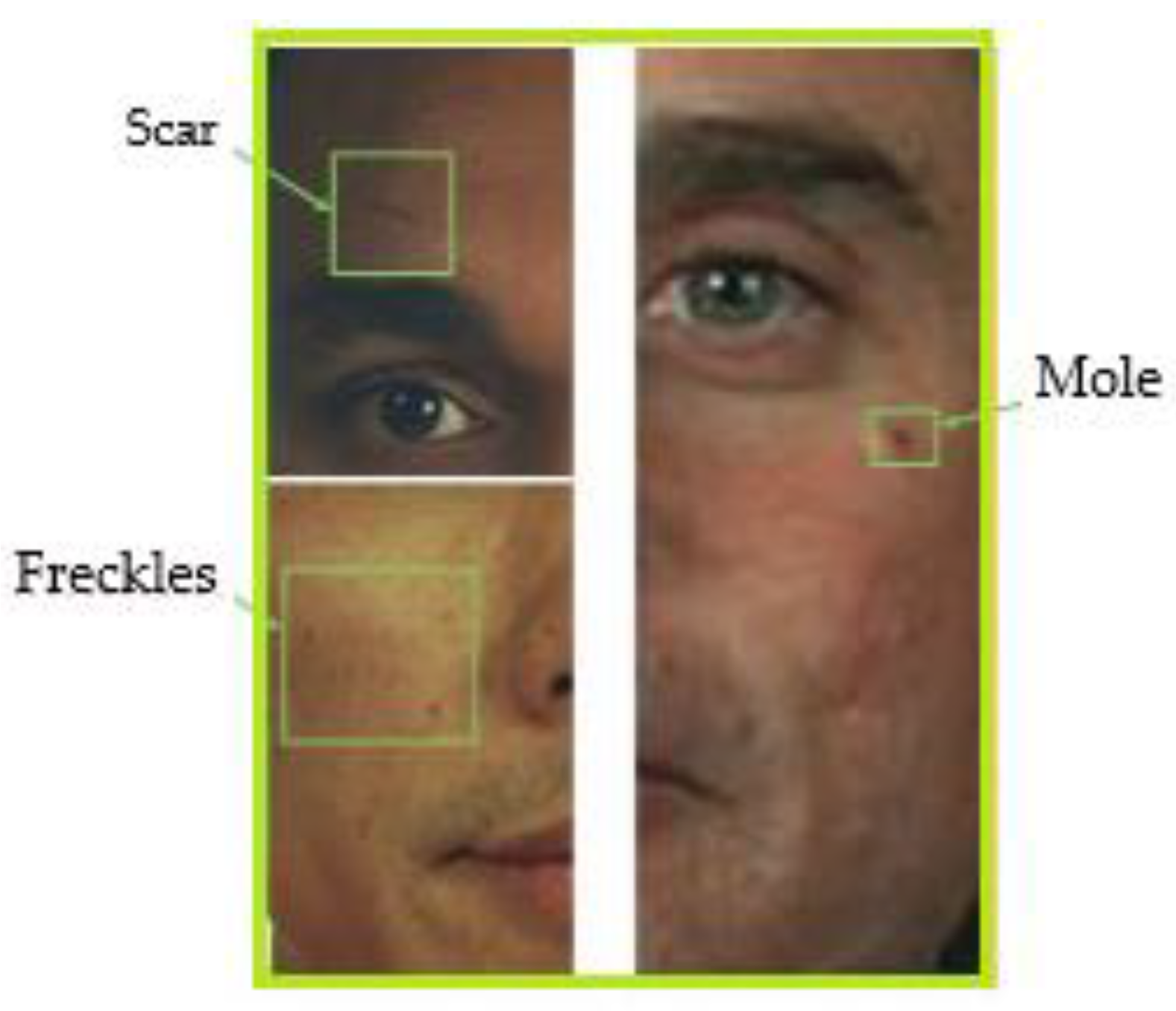
7.6. Face Recognition and Soft Biometrics
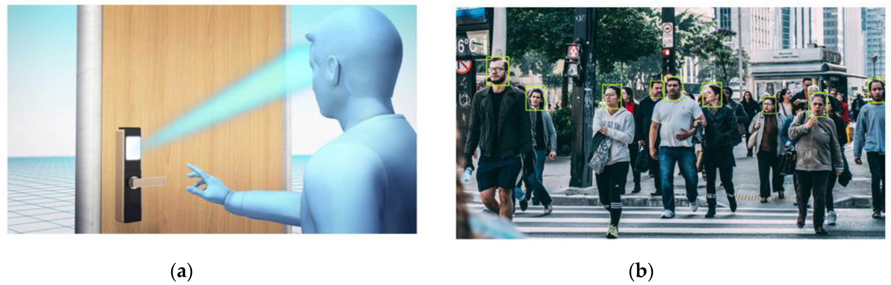
7.7. Face Recognition and Smartphones
7.8. Face Recognition and Internet of Things (IoT)
8. Conclusions
Author Contributions
Funding
Conflicts of Interest
References
- Kortli, Y.; Jridi, M.; Al Falou, A.; Atri, M. A Review of Face Recognition Methods. Sensors 2020, 20, 342. [Google Scholar] [CrossRef] [PubMed] [Green Version]
- O’Toole, A.J.; Roark, D.A.; Abdi, H. Recognizing moving faces: A psychological and neural synthesis. Trends Cogn. Sci. 2002, 6, 261–266. [Google Scholar] [CrossRef]
- Dantcheva, A.; Chen, C.; Ross, A. Can facial cosmetics affect the matching accuracy of face recognition systems? In Proceedings of the 2012 IEEE Fifth International Conference on Biometrics: Theory, Applications and Systems (BTAS), Arlington, VA, USA, 23–27 September 2012; pp. 391–398. [Google Scholar]
- Sinha, P.; Balas, B.; Ostrovsky, Y.; Russell, R. Face recognition by humans: Nineteen results all computer vision researchers should know about. Proc. IEEE 2006, 94, 1948–1962. [Google Scholar] [CrossRef]
- Ouamane, A.; Benakcha, A.; Belahcene, M.; Taleb-Ahmed, A. Multimodal depth and intensity face verification approach using LBP, SLF, BSIF, and LPQ local features fusion. Pattern Recognit. Image Anal. 2015, 25, 603–620. [Google Scholar] [CrossRef]
- Porter, G.; Doran, G. An anatomical and photographic technique for forensic facial identification. Forensic Sci. Int. 2000, 114, 97–105. [Google Scholar] [CrossRef]
- Li, S.Z.; Jain, A.K. Handbook of Face Recognition, 2nd ed.; Springer Publishing Company: New York, NY, USA, 2011. [Google Scholar]
- Morder-Intelligence. Available online: https://www.mordorintelligence.com/industry-reports/facial-recognition-market (accessed on 21 July 2020).
- Guo, G.; Zhang, N. A survey on deep learning based face recognition. Comput. Vis. Image Underst. 2019, 189, 10285. [Google Scholar] [CrossRef]
- Huang, G.B.; Mattar, M.; Berg, T.; Learned-Miller, E. Labeled Faces in the Wild: A Database for Studying Face Recognition in Unconstrained Environments; Technical Report; University of Massachusetts: Amherst, MA, USA, 2007; pp. 7–49. [Google Scholar]
- Bledsoe, W.W. The Model Method in Facial Recognition; Technical Report; Panoramic Research, Inc.: Palo Alto, CA, USA, 1964. [Google Scholar]
- Turk, M.; Pentland, A. Eigenfaces for recognition. J. Cogn. Neurosci. 1991, 3, 71–86. [Google Scholar] [CrossRef]
- Phillips, P.J.; Wechsler, H.; Huang, J.; Rauss, P. The FERET database and evaluation procedure for face recognition algorithms. Image Vis. Comput. 1998, 16, 295–306. [Google Scholar] [CrossRef]
- Phillips, P.J.; Flynn, P.J.; Scruggs, T.; Bowyer, K.W.; Chang, J.; Hoffman, K.; Marques, J.; Min, J.; Worek, W. Overview of the face recognition grand challenge. In Proceedings of the 2005 IEEE Computer Society Conference on Computer Vision and Pattern Recognition (CVPR’05), San Diego, CA, USA, 20–26 June 2005; pp. 947–954. [Google Scholar]
- Taigman, Y.; Yang, M.; Ranzato, M.; Wolf, L. Deepface: Closing the gap to human-level performance in face verification. In Proceedings of the 2014 IEEE Conference on Computer Vision and Pattern Recognition, Columbus, OH, USA, 23–28 June 2014; pp. 1701–1708. [Google Scholar]
- Chihaoui, M.; Elkefi, A.; Bellil, W.; Ben Amar, C. A Survey of 2D Face Recognition Techniques. Computers 2016, 5, 21. [Google Scholar] [CrossRef] [Green Version]
- Benzaoui, A.; Bourouba, H.; Boukrouche, A. System for automatic faces detection. In Proceedings of the 2012 3rd International Conference on Image Processing, Theory, Tools and Applications (IPTA), Istanbul, Turkey, 15–18 October 2012; pp. 354–358. [Google Scholar]
- Martinez, A.M. Recognizing imprecisely localized, partially occluded and expression variant faces from a single sample per class. IEEE Trans. Pattern Anal. Mach. Intell. (PAMI) 2002, 24, 748–763. [Google Scholar] [CrossRef] [Green Version]
- Sidahmed, S.; Messali, Z.; Ouahabi, A.; Trépout, S.; Messaoudi, C.; Marco, S. Nonparametric denoising methods based on contourlet transform with sharp frequency localization: Application to electron microscopy images with low exposure time. Entropy 2015, 17, 2781–2799. [Google Scholar]
- Ouahabi, A. Image Denoising using Wavelets: Application in Medical Imaging. In Advances in Heuristic Signal Processing and Applications; Chatterjee, A., Nobahari, H., Siarry, P., Eds.; Springer: Basel, Switzerland, 2013; pp. 287–313. [Google Scholar]
- Ouahabi, A. A review of wavelet denoising in medical imaging. In Proceedings of the International Workshop on Systems, Signal Processing and Their Applications (IEEE/WOSSPA’13), Algiers, Algeria, 12–15 May 2013; pp. 19–26. [Google Scholar]
- Nakanishi, A.Y.J.; Western, B.J. Advancing the State-of-the-Art in Transportation Security Identification and Verification Technologies: Biometric and Multibiometric Systems. In Proceedings of the 2007 IEEE Intelligent Transportation Systems Conference, Seattle, WA, USA, 30 September–3 October 2007; pp. 1004–1009. [Google Scholar]
- Samaria, F.S.; Harter, A.C. Parameterization of a Stochastic Model for Human Face Identification. In Proceedings of the 1994 IEEE Workshop on Applications of Computer Vision, Sarasota, FL, USA, 5–7 December 1994; pp. 138–142. [Google Scholar]
- Martinez, A.M.; Benavente, R. The AR face database. CVC Tech. Rep. 1998, 24, 1–10. [Google Scholar]
- Messer, K.; Matas, J.; Kittler, J.; Jonsson, K. Xm2vt sdb: The extended m2vts database. In Proceedings of the 1999 2nd International Conference on Audio and Video-based Biometric Person Authentication (AVBPA), Washington, DC, USA, 22–24 March 1999; pp. 72–77. [Google Scholar]
- Bailliére, E.A.; Bengio, S.; Bimbot, F.; Hamouz, M.; Kittler, J.; Mariéthoz, J.; Matas, J.; Messer, K.; Popovici, V.; Porée, F.; et al. The BANCA Database and Evaluation Protocol. In Proceedings of the 2003 International Conference on Audio- and Video-Based Biometric Person Authentication (AVBPA), Guildford, UK, 9–11 June 2003; pp. 625–638. [Google Scholar]
- Huang, G.B.; Jain, V.; Miller, E.L. Unsupervised joint alignment of complex images. In Proceedings of the 2007 IEEE International Conference on Computer Vision (ICCV), Rio de Janeiro, Brazil, 14–20 October 2007; pp. 1–8. [Google Scholar]
- Huang, G.; Mattar, M.; Lee, H.; Miller, E.G.L. Learning to align from scratch. Adv. Neural Inf. Process. Syst. 2012, 25, 764–772. [Google Scholar]
- Gross, R.; Matthews, L.; Cohn, J.; Kanade, T.; Baker, S. Multi-PIE. Image Vis. Comput. 2010, 28, 807–813. [Google Scholar] [CrossRef] [PubMed]
- CASIA Web Face. Available online: http://www.cbsr.ia.ac.cn/english/CASIA-WebFace-Database.html (accessed on 21 July 2019).
- Klare, B.F.; Klein, B.; Taborsky, E.; Blanton, A.; Cheney, J.; Allen, K.; Grother, P.; Mah, A.; Burge, M.; Jain, A.K. Pushing the frontiers of unconstrained face detection and recognition: IARPA Janus Benchmark A. In Proceedings of the 2015 IEEE Conference on Computer Vision and Pattern Recognition (CVPR), Boston, MA, USA, 7–12 June 2015; pp. 1931–1939. [Google Scholar]
- Shlizerman, I.K.; Seitz, S.M.; Miller, D.; Brossard, E. The MegaFace benchmark: 1 million faces for recognition at scale. In Proceedings of the 2016 IEEE Conference on Computer Vision and Pattern Recognition (CVPR), Las Vegas, NV, USA, 26 June–1 July 2016; pp. 4873–4882. [Google Scholar]
- Shlizerman, I.K.; Suwajanakorn, S.; Seitz, S.M. Illumination-aware age progression. In Proceedings of the 2014 IEEE Conference on Computer Vision and Pattern Recognition (CVPR), Columbus, OH, USA, 23–28 June 2014; pp. 3334–3341. [Google Scholar]
- Ng, H.W.; Winkler, S. A data-driven approach to cleaning large face datasets. In Proceedings of the 2014 IEEE International Conference on Image Processing (ICIP), Paris, France, 27–30 October 2014; pp. 343–347. [Google Scholar]
- Sengupta, S.; Cheng, J.; Castillo, C.; Patel, V.M.; Chellappa, R.; Jacobs, D.W. Frontal to Profile Face Verification in the Wild. In Proceedings of the 2016 IEEE Winter Conference on Applications of Computer Vision (WACV), Lake Placid, NY, USA, 7–10 March 2016; pp. 1–9. [Google Scholar]
- Guo, Y.; Zhang, L.; Hu, Y.; He, X.; Gao, J. Ms-Celeb-1m: A dataset and benchmark for large-scale face recognition. In Proceedings of the 14th European Conference on Computer Vision (ECCV), Amsterdam, The Netherlands, 8–16 October 2016. [Google Scholar]
- Wang, T.Y.; Kumar, A. Recognizing Human Faces under Disguise and Makeup. In Proceedings of the 2016 IEEE International Conference on Identity, Security and Behavior Analysis (ISBA), Sendai, Japan, 29 February–2 March 2016; pp. 1–7. [Google Scholar]
- Parkhi, O.M.; Vedaldi, A.; Zisserman, A. Deep Face Recognition. In Proceedings of the 2015 British Machine Vision Conference, Swansea, UK, 7–10 September 2015; pp. 41.1–41.12. [Google Scholar]
- Cao, Q.; Shen, L.; Xie, W.; Parkhi, O.M.; Zisserman, A. VGGFace2: A dataset for recognizing faces across pose and age. In Proceedings of the 2018 13th IEEE International Conference on Automatic Face & Gesture Recognition (FG), Xi’an, China, 15–19 May 2018; pp. 67–74. [Google Scholar]
- Whitelam, C.; Taborsky, E.; Blanton, A.; Maze, B.; Adams, J.; Miller, T.; Kalka, N.; Jain, A.K.; Duncan, J.A.; Allen, K. IARPA Janus Benchmark-B face dataset. In Proceedings of the 2017 IEEE Conference on Computer Vision and Pattern Recognition Workshops (CVPRW), Honolulu, HI, USA, 21–26 July 2017; pp. 592–600. [Google Scholar]
- Nech, A.; Shlizerman, I.K. Level playing field for million scale face recognition. In Proceedings of the 2017 IEEE Conference on Computer Vision and Pattern Recognition (CVPR), Honolulu, HI, USA, 21–26 July 2017; pp. 3406–3415. [Google Scholar]
- Kushwaha, V.; Singh, M.; Singh, R.; Vatsa, M. Disguised Faces in the Wild. In Proceedings of the 2018 IEEE/CVF Conference on Computer Vision and Pattern Recognition Workshops (CVPRW), Salt Lake City, UT, USA, 18–22 June 2018; pp. 1–18. [Google Scholar]
- Maze, B.; Adams, J.; Duncan, J.A.; Kalka, N.; Miller, T.; Otto, C.; Jain, A.K.; Niggel, W.T.; Anderson, J.; Cheney, J.; et al. IARPA Janus benchmark-C: Face dataset and protocol. In Proceedings of the 2018 International Conference on Biometrics (ICB), Gold Coast, QLD, Australia, 20–23 February 2018; pp. 158–165. [Google Scholar]
- Elharrouss, O.; Almaadeed, N.; Al-Maadeed, S. LFR face dataset: Left-Front-Right dataset for pose-invariant face recognition in the wild. In Proceedings of the 2020 IEEE International Conference on Informatics, IoT, and Enabling Technologies (ICIoT), Doha, Qatar, 2–5 February 2020; pp. 124–130. [Google Scholar]
- Wang, Z.; Wang, G.; Huang, B.; Xiong, Z.; Hong, Q.; Wu, H.; Yi, P.; Jiang, K.; Wang, N.; Pei, Y.; et al. Masked Face Recognition Dataset and Application. arXiv 2020, arXiv:2003.09093v2. [Google Scholar]
- Belhumeur, P.N.; Hespanha, J.P.; Kriegman, D.J. Eigenfaces vs Fisherfaces: Recognition using class specific linear projection. IEEE Trans. Pattern Anal. Mach. Intell. (PAMI) 1997, 19, 711–720. [Google Scholar] [CrossRef] [Green Version]
- Stone, J.V. Independent component analysis: An introduction. Trends Cogn. Sci. 2002, 6, 59–64. [Google Scholar] [CrossRef]
- Sirovich, L.; Kirby, M. Low-Dimensional procedure for the characterization of human faces. J. Opt. Soc. Am. 1987, 4, 519–524. [Google Scholar] [CrossRef]
- Kirby, M.; Sirovich, L. Application of the Karhunen-Loève procedure for the characterization of human faces. IEEE Trans. Pattern Anal. Mach. Intell. (PAMI) 1990, 12, 831–835. [Google Scholar] [CrossRef] [Green Version]
- Femmam, S.; M’Sirdi, N.K.; Ouahabi, A. Perception and characterization of materials using signal processing techniques. IEEE Trans. Instrum. Meas. 2001, 50, 1203–1211. [Google Scholar] [CrossRef]
- Zhao, L.; Yang, Y.H. Theoretical analysis of illumination in PCA-based vision systems. Pattern Recognit. 1999, 32, 547–564. [Google Scholar] [CrossRef]
- Pentland, A.; Moghaddam, B.; Starner, T. View-Based and modular eigenspaces for face recognition. In Proceedings of the 1994 IEEE Conference on Computer Vision and Pattern Recognition (CVPR), Seattle, WA, USA, 21–23 June 1994; pp. 84–91. [Google Scholar]
- Bartlett, M.; Movellan, J.; Sejnowski, T. Face Recognition by Independent Component Analysis. IEEE Trans. Neural Netw. 2002, 13, 1450–1464. [Google Scholar] [CrossRef]
- Abhishree, T.M.; Latha, J.; Manikantan, K.; Ramachandran, S. Face recognition using Gabor Filter based feature extraction with anisotropic diffusion as a pre-processing technique. Procedia Comput. Sci. 2015, 45, 312–321. [Google Scholar] [CrossRef] [Green Version]
- Zehani, S.; Ouahabi, A.; Oussalah, M.; Mimi, M.; Taleb-Ahmed, A. Trabecular bone microarchitecture characterization based on fractal model in spatial frequency domain imaging. Int. J. Imaging Syst. Technol. accepted.
- Ouahabi, A. Signal and Image Multiresolution Analysis, 1st ed.; ISTE-Wiley: London, UK, 2012. [Google Scholar]
- Guetbi, C.; Kouame, D.; Ouahabi, A.; Chemla, J.P. Methods based on wavelets for time delay estimation of ultrasound signals. In Proceedings of the 1998 IEEE International Conference on Electronics, Circuits and Systems, Lisbon, Portugal, 7–10 September 1998; pp. 113–116. [Google Scholar]
- Ferroukhi, M.; Ouahabi, A.; Attari, M.; Habchi, Y.; Taleb-Ahmed, A. Medical video coding based on 2nd-generation wavelets: Performance evaluation. Electronics 2019, 8, 88. [Google Scholar] [CrossRef] [Green Version]
- Wang, M.; Jiang, H.; Li, Y. Face recognition based on DWT/DCT and SVM. In Proceedings of the 2010 International Conference on Computer Application and System Modeling (ICCASM), Taiyuan, China, 22–24 October 2010; pp. 507–510. [Google Scholar]
- Bookstein, F.L. Principal warps: Thin-plate splines and the decomposition of deformations. IEEE Trans. Pattern Anal. Mach. Intell. (PAMI) 1989, 11, 567–585. [Google Scholar] [CrossRef] [Green Version]
- Shih, F.Y.; Chuang, C. Automatic extraction of head and face boundaries and facial features. Inf. Sci. 2004, 158, 117–130. [Google Scholar] [CrossRef]
- Zobel, M.; Gebhard, A.; Paulus, D.; Denzler, J.; Niemann, H. Robust facial feature localization by coupled features. In Proceedings of the 2000 4th IEEE International Conference on Automatic Face and Gesture Recognition (FG), Grenoble, France, 26–30 March 2000; pp. 2–7. [Google Scholar]
- Wiskott, L.; Fellous, J.M.; Malsburg, C.V.D. Face recognition by elastic bunch graph matching. IEEE Trans. Pattern Anal. Mach. Intell. (PAMI) 1997, 19, 775–779. [Google Scholar] [CrossRef]
- Xue, Z.; Li, S.Z.; Teoh, E.K. Bayesian shape model for facial feature extraction and recognition. Pattern Recognit. 2003, 36, 2819–2833. [Google Scholar] [CrossRef]
- Tistarelli, M. Active/space-variant object recognition. Image Vis. Comput. 1995, 13, 215–226. [Google Scholar] [CrossRef]
- Lades, M.; Vorbuggen, J.C.; Buhmann, J.; Lange, J.; Malsburg, C.V.D.; Wurtz, R.P.; Konen, W. Distortion invariant object recognition in the dynamic link architecture. IEEE Trans. Comput. 1993, 42, 300–311. [Google Scholar] [CrossRef] [Green Version]
- Wiskott, L. Phantom faces for face analysis. Pattern Recognit. 1997, 30, 837–846. [Google Scholar] [CrossRef]
- Duc, B.; Fischer, S.; Bigun, J. Face authentication with Gabor information on deformable graphs. IEEE Trans. Image Process. 1999, 8, 504–516. [Google Scholar] [CrossRef] [PubMed] [Green Version]
- Kotropoulos, C.; Tefas, A.; Pitas, I. Frontal face authentication using morphological elastic graph matching. IEEE Trans. Image Process. 2000, 9, 555–560. [Google Scholar] [CrossRef] [PubMed]
- Jackway, P.T.; Deriche, M. Scale-space properties of the multiscale morphological dilation-erosion. IEEE Trans. Pattern Anal. Mach. Intell. (PAMI) 1996, 18, 38–51. [Google Scholar] [CrossRef] [Green Version]
- Tefas, A.; Kotropoulos, C.; Pitas, I. Face verification using elastic graph matching based on morphological signal decomposition. Signal Process. 2002, 82, 833–851. [Google Scholar] [CrossRef]
- Kumar, D.; Garaina, J.; Kisku, D.R.; Sing, J.K.; Gupta, P. Unconstrained and Constrained Face Recognition Using Dense Local Descriptor with Ensemble Framework. Neurocomputing 2020. [Google Scholar] [CrossRef]
- Zehani, S.; Ouahabi, A.; Mimi, M.; Taleb-Ahmed, A. Staistical features extraction in wavelet domain for texture classification. In Proceedings of the 2019 6th International Conference on Image and Signal Processing and their Applications (IEEE/ISPA), Mostaganem, Algeria, 24–25 November 2019; pp. 1–5. [Google Scholar]
- Ait Aouit, D.; Ouahabi, A. Nonlinear Fracture Signal Analysis Using Multifractal Approach Combined with Wavelet. Fractals Complex Geom. Patterns Scaling Nat. Soc. 2011, 19, 175–183. [Google Scholar] [CrossRef]
- Girault, J.M.; Kouame, D.; Ouahabi, A. Analytical formulation of the fractal dimension of filtered stochastic signal. Signal Process. 2010, 90, 2690–2697. [Google Scholar] [CrossRef] [Green Version]
- Djeddi, M.; Ouahabi, A.; Batatia, H.; Basarab, A.; Kouamé, D. Discrete wavelet transform for multifractal texture classification: Application to ultrasound imaging. In Proceedings of the IEEE International Conference on Image Processing (IEEE ICIP2010), Hong Kong, China, 26–29 September 2010; pp. 637–640. [Google Scholar]
- Ouahabi, A. Multifractal analysis for texture characterization: A new approach based on DWT. In Proceedings of the 10th International Conference on Information Science, Signal Processing and Their Applications (IEEE/ISSPA), Kuala Lumpur, Malaysia, 10–13 May 2010; pp. 698–703. [Google Scholar]
- Davies, E.R. Introduction to texture analysis. In Handbook of Texture Analysis; Mirmehdi, M., Xie, X., Suri, J., Eds.; Imperial College Press: London, UK, 2008; pp. 1–31. [Google Scholar]
- Benzaoui, A.; Hadid, A.; Boukrouche, A. Ear biometric recognition using local texture descriptors. J. Electron. Imaging 2014, 23, 053008. [Google Scholar] [CrossRef]
- Ahonen, T.; Hadid, A.; Pietikäinen, M. Face recognition with local binary patterns. In Proceedings of the 8th European Conference on Computer Vision (ECCV), Prague, Czech Republic, 11–14 May 2004; pp. 469–481. [Google Scholar]
- Ahonen, T.; Hadid, A.; Pietikäinen, M. Face description with local binary patterns: Application to face recognition. IEEE Trans. Pattern Anal. Mach. Intell. 2006, 28, 2037–2041. [Google Scholar] [CrossRef]
- Beveridge, J.R.; Bolme, D.; Draper, B.A.; Teixeira, M. The CSU face identification evaluation system: Its purpose, features, and structure. Mach. Vis. Appl. 2005, 16, 128–138. [Google Scholar] [CrossRef]
- Moghaddam, B.; Nastar, C.; Pentland, A. A bayesian similarity measure for direct image matching. In Proceedings of the 13th International Conference on Pattern Recognition (ICPR), Vienna, Austria, 25–29 August 1996; pp. 350–358. [Google Scholar]
- Rodriguez, Y.; Marcel, S. Face authentication using adapted local binary pattern histograms. In Proceedings of the 9th European Conference on Computer Vision (ECCV), Graz, Austria, 7–13 May 2006; pp. 321–332. [Google Scholar]
- Sadeghi, M.; Kittler, J.; Kostin, A.; Messer, K. A comparative study of automatic face verification algorithms on the banca database. In Proceedings of the 4th International Conference on Audio- and Video-Based Biometric Person Authentication (AVBPA), Guilford, UK, 9–11 June 2003; pp. 35–43. [Google Scholar]
- Huang, X.; Li, S.Z.; Wang, Y. Jensen-shannon boosting learning for object recognition. In Proceedings of the IEEE International Conference on Computer Vision and Pattern Recognition (CVPR), San Diego, CA, USA, 20–26 June 2005; pp. 144–149. [Google Scholar]
- Boutella, E.; Harizi, F.; Bengherabi, M.; Ait-Aoudia, S.; Hadid, A. Face verification using local binary patterns and generic model adaptation. Int. J. Biomed. 2015, 7, 31–44. [Google Scholar] [CrossRef]
- Benzaoui, A.; Boukrouche, A. 1DLBP and PCA for face recognition. In Proceedings of the 2013 11th International Symposium on Programming and Systems (ISPS), Algiers, Algeria, 22–24 April 2013; pp. 7–11. [Google Scholar]
- Benzaoui, A.; Boukrouche, A. Face Recognition using 1DLBP Texture Analysis. In Proceedings of the 5th International Conference of Future Computational Technologies and Applications, Valencia, Spain, 27 May–1 June 2013; pp. 14–19. [Google Scholar]
- Benzaoui, A.; Boukrouche, A. Face Analysis, Description, and Recognition using Improved Local Binary Patterns in One Dimensional Space. J. Control Eng. Appl. Inform. (CEAI) 2014, 16, 52–60. [Google Scholar]
- Ahonen, T.; Rathu, E.; Ojansivu, V.; Heikkilä, J. Recognition of Blurred Faces Using Local Phase Quantization. In Proceedings of the 19th International Conference on Pattern Recognition (ICPR), Tampa, FL, USA, 8–11 December 2008; pp. 1–4. [Google Scholar]
- Ojansivu, V.; Heikkil, J. Blur insensitive texture classification using local phase quantization. In Proceedings of the 3rd International Conference on Image and Signal Processing (ICSIP), Cherbourg-Octeville, France, 1–3 July 2008; pp. 236–243. [Google Scholar]
- Tan, X.; Triggs, B. Enhanced local texture feature sets for face recognition under difficult lighting conditions. In Proceedings of the 3rd International Workshop on Analysis and Modeling of Faces and Gestures (AMFG), Rio de Janeiro, Brazil, 20 October 2007; pp. 168–182. [Google Scholar]
- Lei, Z.; Ahonen, T.; Pietikainen, M.; Li, S.Z. Local Frequency Descriptor for Low-Resolution Face Recognition. In Proceedings of the 9th Conference on Automatic Face and Gesture Recognition (FG), Santa Barbara, CA, USA, 21–25 March 2011; pp. 161–166. [Google Scholar]
- Kannala, J.; Rahtu, E. BSIF: Binarized statistical image features. In Proceedings of the 21th International Conference on Pattern Recognition (ICPR), Tsukuba, Japan, 11–15 November 2012; pp. 1363–1366. [Google Scholar]
- Schmidhuber, J. Deep Learning in Neural Networks: An Overview. Neural Netw. 2015, 61, 85–117. [Google Scholar] [CrossRef] [PubMed] [Green Version]
- Deng, L. A tutorial survey of architectures, algorithms, and applications for deep learning. APSIPA Trans. Signal Inf. Process. 2014, 3, 1–29. [Google Scholar] [CrossRef] [Green Version]
- Deng, L.; Yu, D. Deep Learning: Methods and Applications. Found. Trends Signal Process. 2014, 7, 197–387. [Google Scholar] [CrossRef] [Green Version]
- Vincent, P.; Larochelle, H.; Lajoie, I.; Bengio, Y.; Manzagol, P.A. Stacked denoising autoencoders: Learning useful representations in a deep network with a local denoising criterion. J. Mach. Learn. Res. 2010, 11, 3371–3408. [Google Scholar]
- Salakhutdinov, R.; Hinton, G. Deep Boltzmann machines. In Proceedings of the 12th International Conference on Artificial Intelligence and Statistics, Clearwater, FL, USA, 16–19 April 2009; pp. 448–455. [Google Scholar]
- Sutskever, I.; Martens, J.; Hinton, G. Generating text with recurrent neural networks. In Proceedings of the 28th International Conference on Machine Learning (ICML), Bellevue, WA, USA, 28 June–2 July 2011; pp. 1017–1024. [Google Scholar]
- Poon, H.; Domingos, P. Sum-product networks: A new deep architecture. In Proceedings of the 2011 IEEE International Conference on Computer Vision Workshops (ICCV Workshops), Barcelona, Spain, 6–13 November 2011; pp. 689–690. [Google Scholar]
- Kimb, K.; Aminantoa, M.E. Deep Learning in Intrusion Detection Perspective: Overview and further Challenges. In Proceedings of the International Workshop on Big Data and Information Security (IWBIS), Jakarta, Indonesia, 23–24 September 2017; pp. 5–10. [Google Scholar]
- Ouahabi, A. Analyse spectrale paramétrique de signaux lacunaires. Traitement Signal 1992, 9, 181–191. [Google Scholar]
- Ouahabi, A.; Lacoume, J.-L. New results in spectral estimation of decimated processes. IEEE Electron. Lett. 1991, 27, 1430–1432. [Google Scholar] [CrossRef]
- Scherer, D.; Müller, A.; Behnke, S. Evaluation of pooling operations in convolutional architectures for object recognition. In Proceedings of the 2010 International Conference on Artificial Neural Networks, Thessaloniki, Greece, 15–18 September 2010; pp. 92–101. [Google Scholar]
- Coşkun, M.; Uçar, A.; Yildirim, Ö.; Demir, Y. Face recognition based on convolutional neural network. In Proceedings of the 2017 International Conference on Modern Electrical and Energy Systems (MEES), Kremenchuk, Ukraine, 15–17 November 2017; pp. 376–379. [Google Scholar]
- Lecun, Y.; Bottou, L.; Bengio, Y.; Haffner, P. Gradient-based learning applied to document recognition. Proc. IEEE 1998, 86, 2278–2324. [Google Scholar] [CrossRef] [Green Version]
- Russakovsky, O.; Deng, J.; Su, H.; Krause, J.; Satheesh, S.; Ma, S.; Huang, Z.; Karpathy, A.; Khosla, A.; Bernstein, M.; et al. ImageNet Large Scale Visual Recognition Challenge. Int. J. Comput. Vis. 2015, 115, 211–252. [Google Scholar] [CrossRef] [Green Version]
- Krizhevsky, A.; Sutskever, I.; Hinton, G.E. ImageNet classification with deep convolutional neural networks. In Proceedings of the 25th International Conference on Neural Information Processing Systems (NIPS), Lake Tahoe, NV, USA, 3–6 December 2012; pp. 1097–1105. [Google Scholar]
- Simonyan, K.; Zisserman, A. Very deep convolutional networks for large-scale image recognition. In Proceedings of the 2nd International Conference on Learning Representations (ICLR), Banff, AB, Canada, 14–16 April 2014. [Google Scholar]
- Szegedy, C.; Liu, W.; Jia, Y.; Sermanet, P.; Reed, S.; Anguelov, D.; Erhan, D.; Vanhoucke, V.; Rabinovich, A. Going deeper with convolutions. In Proceedings of the 2015 IEEE Conference on Computer Vision and Pattern Recognition (CVPR), Boston, MA, USA, 7–12 June 2015; pp. 1–9. [Google Scholar]
- He, K.; Zhang, X.; Ren, S.; Sun, J. Deep residual learning for image recognition. In Proceedings of the 2016 IEEE Conference on Computer Vision and Pattern Recognition (CVPR), Las Vegas, NV, USA, 27–30 June 2016; pp. 770–778. [Google Scholar]
- Hu, J.; Shen, L.; Albanie, S.; Sun, G.; Wu, E. Squeeze-and-excitation networks. IEEE Trans. Pattern Anal. Mach. Intell. (PAMI) 2019, 42, 7132–7141. [Google Scholar]
- Chopra, S.; Hadsell, R.; LeCun, Y. Learning a similarity metric discriminatively, with application to face verification. In Proceedings of the 2005 IEEE Computer Society Conference on Computer Vision and Pattern Recognition, San Diego, CA, USA, 20–26 June 2005; pp. 539–546. [Google Scholar]
- Sun, Y.; Wang, X.; Tang, X. Deep learning face representation from predicting 10,000 classes. In Proceedings of the 2014 IEEE Conference on Computer Vision and Pattern Recognition, Columbus, OH, USA, 23–28 June 2014; pp. 1891–1898. [Google Scholar]
- Sun, Y.; Chen, Y.; Wang, X.; Tang, X. Deep learning face representation by joint identification-verification. In Proceedings of the 27th International Conference on Neural Information Processing Systems, Montreal, QC, Canada, 8–13 December 2014; pp. 1988–1996. [Google Scholar]
- Sun, Y.; Wang, X.; Tang, X. Deeply learned face representations are sparse, selective, and robust. In Proceedings of the 2015 IEEE Conference on Computer Vision and Pattern Recognition (CVPR), Boston, MA, USA, 7–12 June 2015; pp. 2892–2900. [Google Scholar]
- Sun, Y.; Liang, D.; Wang, X.; Tang, X. DeepID3: Face Recognition with Very Deep Neural Networks. arXiv 2015, arXiv:1502.00873v1. [Google Scholar]
- Taigman, Y.; Yang, M.; Ranzato, M.; Wolf, L. Web-Scale training for face identification. In Proceedings of the 2015 IEEE Conference on Computer Vision and Pattern Recognition (CVPR), Boston, MA, USA, 7–12 June 2015; pp. 2746–2754. [Google Scholar]
- Ouahabi, A.; Depollier, C.; Simon, L.; Kouame, D. Spectrum estimation from randomly sampled velocity data [LDV]. IEEE Trans. Instrum. Meas. 1998, 47, 1005–1012. [Google Scholar] [CrossRef]
- Liu, J.; Deng, Y.; Bai, T.; Huang, C. Targeting ultimate accuracy: Face recognition via deep embedding. arXiv 2015, arXiv:1506.07310v4. [Google Scholar]
- Masi, I.; Tran, A.T.; Hassner, T.; Leksut, J.T.; Medioni, G. Do we really need to collect millions of faces for effective face recognition? In Proceedings of the 2016 European Conference on Computer Vision (ECCV), Amsterdam, The Netherland, 8–16 October 2016; pp. 579–596. [Google Scholar]
- Zhang, X.; Fang, Z.; Wen, Y.; Li, Z.; Qiao, Y. Range loss for deep face recognition with Long-Tailed Training Data. In Proceedings of the 2017 IEEE International Conference on Computer Vision (ICCV), Venice, Italy, 22–29 October 2017; pp. 5419–5428. [Google Scholar]
- Liu, W.; Wen, Y.; Yu, Z.; Yang, M. Large-margin softmax loss for convolutional neural networks. In Proceedings of the 33rd International Conference on Machine Learning, New York, NY, USA, 19–24 June 2016; pp. 507–516. [Google Scholar]
- Chen, B.; Deng, W.; Du, J. Noisy Softmax: Improving the Generalization Ability of DCNN via Postponing the Early Softmax Saturation. In Proceedings of the 2017 IEEE Conference on Computer Vision and Pattern Recognition (CVPR), Honolulu, HI, USA, 21–26 July 2017; pp. 4021–4030. [Google Scholar]
- Schroff, F.; Kalenichenko, D.; Philbin, J. FaceNet: A unified embedding for face recognition and clustering. In Proceedings of the 2015 IEEE Conference on Computer Vision and Pattern Recognition (CVPR), Boston, MA, USA, 7–12 June 2015; pp. 815–823. [Google Scholar]
- Zeiler, M.D.; Fergus, R. Visualizing and understanding convolutional networks. arXiv 2013, arXiv:1311.2901v3. [Google Scholar]
- Ben Fredj, H.; Bouguezzi, S.; Souani, C. Face recognition in unconstrained environment with CNN. Vis. Comput. 2020, 1–10. [Google Scholar] [CrossRef]
- Wen, Y.; Zhang, K.; Li, Z.; Qiao, Y. A discriminative feature learning approach for deep face recognition. In Proceedings of the 14th European Conference on Computer Vision (ECCV), Amsterdam, The Netherlands, 8–16 October 2016; pp. 499–515. [Google Scholar]
- Wu, Y.; Liu, H.; Li, J.; Fu, Y. Deep Face Recognition with Center Invariant Loss. In Proceedings of the Thematic Workshop of ACM Multimedia, Mountain View, CA, USA, 23–27 October 2017; pp. 408–414. [Google Scholar]
- Yin, X.; Yu, X.; Sohn, K.; Liu, X.; Chandraker, M. Feature Transfer Learning for Face Recognition with Under-Represented Data. In Proceedings of the 2019 International Conference on Computer Vision and Pattern Recognition (CVPR), Long Beach, CA, USA, 16–20 June 2019. [Google Scholar]
- Ranjan, R.; Castillo, C.D.; Chellappa, R. L2-constrained softmax loss for discriminative face verification. arXiv 2017, arXiv:1703.09507v3. [Google Scholar]
- Deng, J.; Zhou, Y.; Zafeiriou, S. Marginal Loss for Deep Face Recognition. In Proceedings of the 2017 IEEE Conference on Computer Vision and Pattern Recognition Workshops (CVPRW), Honolulu, HI, USA, 21–26 July 2017; pp. 2006–2014. [Google Scholar]
- Wang, F.; Xiang, X.; Cheng, J.; Yuille, A.L. NormFace: L2 Hypersphere Embedding for Face Verification. In Proceedings of the 25th ACM International Conference on Multimedia, Mountain View, CA, USA, 23–27 October 2017; pp. 1041–1049. [Google Scholar]
- Liu, Y.; Li, H.; Wang, X. Rethinking Feature Discrimination and Polymerization for Large-Scale Recognition. In Proceedings of the 31st Conference on Neural Information Processing Systems (NIPS), (Deep Learning Workshop), Long Beach, CA, USA, 4–9 December 2017. [Google Scholar]
- Hasnat, M.; Bohné, J.; Milgram, J.; Gentric, S.; Chen, L. Von Mises-Fisher Mixture Model-based Deep Learning: Application to Face Verification. arXiv 2017, arXiv:1706.04264v2. [Google Scholar]
- Liu, W.; Wen, Y.; Yu, Z.; Li, M.; Raj, B.; Song, L. SphereFace: Deep Hypersphere Embedding for Face Recognition. In Proceedings of the 2017 IEEE Conference on Computer Vision and Pattern Recognition (CVPR), Honolulu, HI, USA, 21–26 July 2017; pp. 6738–6746. [Google Scholar]
- Zheng, Y.; Pal, D.K.; Savvides, M. Ring Loss: Convex Feature Normalization for Face Recognition. In Proceedings of the 2018 IEEE/CVF Conference on Computer Vision and Pattern Recognition, Salt Lake City, UT, USA, 18–22 June 2018; pp. 5089–5097. [Google Scholar]
- Guo, Y.; Zhang, L. One-Shot Face Recognition by Promoting Underrepresented Classes. arXiv 2018, arXiv:1707.05574v2. [Google Scholar]
- Wang, H.; Wang, Y.; Zhou, Z.; Ji, X.; Gong, D.; Zhou, J.; Liu, W. CosFace: Large Margin Cosine Loss for Deep Face Recognition. In Proceedings of the 2018 IEEE/CVF Conference on Computer Vision and Pattern Recognition, Salt Lake City, UT, USA, 18–22 June 2018; pp. 5265–5274. [Google Scholar]
- Wang, F.; Cheng, J.; Liu, W.; Liu, H. Additive Margin Softmax for Face Verification. IEEE Signal Process. Lett. 2018, 25, 926–930. [Google Scholar] [CrossRef] [Green Version]
- Wu, X.; He, R.; Sun, Z.; Tan, T. A Light CNN for Deep Face Representation with Noisy Labels. IEEE Trans. Inf. Forensics Secur. 2018, 13, 2884–2896. [Google Scholar] [CrossRef] [Green Version]
- Hayat, M.; Khan, S.H.; Zamir, W.; Shen, J.; Shao, L. Gaussian Affinity for Max-margin Class Imbalanced Learning. In Proceedings of the 2019 International Conference on Computer Vision (ICCV), Seoul, Korea, 27 October–2 November 2019. [Google Scholar]
- Deng, J.; Guo, J.; Zafeiriou, S. ArcFace: Additive Angular Margin Loss for Deep Face Recognition. In Proceedings of the 2019 International Conference on Computer Vision and Pattern Recognition (CVPR), Lone Beach, CA, USA, 16–20 June 2019; pp. 4690–4699. [Google Scholar]
- Huang, C.; Li, Y.; Loy, C.C.; Tang, X. Deep Imbalanced Learning for Face Recognition and Attribute Prediction. IEEE Trans. Pattern Anal. Mach. Intell. (PAMI) 2019. Available online: https://ieeexplore.ieee.org/document/8708977 (accessed on 21 July 2020).
- Song, L.; Gong, D.; Li, Z.; Liu, C.; Liu, W. Occlusion Robust Face Recognition Based on Mask Learning with Pairwise Differential Siamese Network. In Proceedings of the 2019 International Conference on Computer Vision (ICCV), Seoul, Korea, 27 October–2 November 2019. [Google Scholar]
- Wei, X.; Wang, H.; Scotney, B.; Wan, H. Minimum margin loss for deep face recognition. Pattern Recognit. 2020, 97, 107012. [Google Scholar] [CrossRef]
- Sun, J.; Yang, W.; Gao, R.; Xue, J.H.; Liao, Q. Inter-class angular margin loss for face recognition. Signal Process. Image Commun. 2020, 80, 115636. [Google Scholar] [CrossRef]
- Wu, Y.; Wu, Y.; Wu, R.; Gong, Y.; Lv, K.; Chen, K.; Liang, D.; Hu, X.; Liu, X.; Yan, J. Rotation consistent margin loss for efficient low-bit face recognition. In Proceedings of the 2020 IEEE/CVF Conference on Computer Vision and Pattern Recognition (CVPR), Seattle, WA, USA, 16–18 June 2020; pp. 6866–6876. [Google Scholar]
- Ling, H.; Wu, J.; Huang, J.; Li, P. Attention-based convolutional neural network for deep face recognition. Multimed. Tools Appl. 2020, 79, 5595–5616. [Google Scholar] [CrossRef]
- Wu, B.; Wu, H. Angular Discriminative Deep Feature Learning for Face Verification. In Proceedings of the 2020 IEEE International Conference on Acoustics, Speech and Signal Processing (ICASSP), Barcelona, Spain, 4–8 May 2020; pp. 2133–2137. [Google Scholar]
- Chen, D.; Cao, X.; Wang, L.; Wen, F.; Sun, J. Bayesian face revisited: A joint formulation. In Proceedings of the European Conference on Computer Vision (ECCV), Firenze, Italy, 7–13 October 2012; pp. 566–579. [Google Scholar]
- Chen, B.C.; Chen, C.S.; Hsu, W.H. Face recognition and retrieval using cross-age reference coding with cross-age celebrity dataset. IEEE Trans. Multimed. 2015, 17, 804–815. [Google Scholar] [CrossRef]
- Liu, Z.; Luo, P.; Wang, X.; Tang, X. Deep learning face attributes in the wild. In Proceedings of the 2015 IEEE International Conference on Computer Vision (ICCV), Santiago, Chile, 11–18 December 2015; pp. 3730–3738. [Google Scholar]
- Szegedy, C.; Ioffe, S.; Vanhoucke, V.; Alemi, A.A. Inception-v4, inception-resnet and the impact of residual connections on learning. In Proceedings of the Thirty-First AAAI Conference on Artificial Intelligence, San Francisco, CA, USA, 4–9 February 2017; pp. 4278–4284. [Google Scholar]
- Oumane, A.; Belahcene, M.; Benakcha, A.; Bourennane, S.; Taleb-Ahmed, A. Robust Multimodal 2D and 3D Face Authentication using Local Feature Fusion. Signal Image Video Process. 2016, 10, 12–137. [Google Scholar] [CrossRef]
- Oumane, A.; Boutella, E.; Benghherabi, M.; Taleb-Ahmed, A.; Hadid, A. A Novel Statistical and Multiscale Local Binary Feature for 2D and 3D Face Verification. Comput. Electr. Eng. 2017, 62, 68–80. [Google Scholar] [CrossRef]
- Soltanpour, S.; Boufama, B.; Wu, Q.M.J. A survey of local feature methods for 3D face recognition. Pattern Recognit. 2017, 72, 391–406. [Google Scholar] [CrossRef]
- Zhou, S.; Xiao, S. 3D Face Recognition: A Survey. Hum. Cent. Comput. Inf. Sci. 2018, 8, 8–35. [Google Scholar] [CrossRef] [Green Version]
- Min, R.; Kose, N.; Dugelay, J. KinectFaceDB: A Kinect Database for Face Recognition. IEEE Trans. Syst. Man Cybern. Syst. 2014, 44, 1534–1548. [Google Scholar] [CrossRef]
- Drira, H.; Ben Amor, B.; Srivastava, A.; Daoudi, M.; Slama, R. 3D Face Recognition under Expressions, Occlusions, and Pose Variations. IEEE Trans. Pattern Anal. Mach. Intell. 2013, 35, 2270–2283. [Google Scholar] [CrossRef] [PubMed] [Green Version]
- Ribeiro Alexandre, G.; Marques Soares, J.; Pereira Thé, G.A. Systematic review of 3D facial expression recognition methods. Pattern Recognit. 2020, 100, 107108. [Google Scholar] [CrossRef]
- Ríos-Sánchez, B.; Costa-da-Silva, D.; Martín-Yuste, N.; Sánchez-Ávila, C. Deep Learning for Facial Recognition on Single Sample per Person Scenarios with Varied Capturing Conditions. Appl. Sci. 2019, 9, 5474. [Google Scholar]
- Kim, D.; Hernandez, M.; Choi, J.; Medioni, G. Deep 3D face identification. In Proceedings of the IEEE International Joint Conference on Biometrics (IJCB), Denver, CO, USA, 1–4 October 2017; pp. 133–142. [Google Scholar]
- Gilani, S.Z.; Mian, A.; Eastwood, P. Deep, dense and accurate 3D face correspondence for generating population specific deformable models. Pattern Recognit. 2017, 69, 238–250. [Google Scholar] [CrossRef] [Green Version]
- Gilani, S.Z.; Mian, A.; Shafait, F.; Reid, I. Dense 3D face correspondence. IEEE Trans. Pattern Anal. Mach. Intell. (TPAMI) 2018, 40, 1584–1598. [Google Scholar] [CrossRef] [PubMed] [Green Version]
- Gilani, S.Z.; Mian, A. Learning from Millions of 3D Scans for Large-scale 3D Face Recognition. In Proceedings of the 2018 IEEE/CVF Conference on Computer Vision and Pattern Recognition, Salt Lake City, UT, USA, 18–22 June 2018; pp. 1896–1905. [Google Scholar]
- Mimouna, A.; Alouani, I.; Ben Khalifa, A.; El Hillali, Y.; Taleb-Ahmed, A.; Menhaj, A.; Ouahabi, A.; Ben Amara, N.E. OLIMP: A Heterogeneous Multimodal Dataset for Advanced Environment Perception. Electronics 2020, 9, 560. [Google Scholar] [CrossRef] [Green Version]
- Benzaoui, A.; Boukrouche, A.; Doghmane, H.; Bourouba, H. Face recognition using 1DLBP, DWT, and SVM. In Proceedings of the 2015 3rd International Conference on Control, Engineering & Information Technology (CEIT), Tlemcen, Algeria, 25–27 May 2015; pp. 1–6. [Google Scholar]
- Ait Aouit, D.; Ouahabi, A. Monitoring crack growth using thermography.-Suivi de fissuration de matériaux par thermographie. C. R. Mécanique 2008, 336, 677–683. [Google Scholar] [CrossRef]
- Arya, S.; Pratap, N.; Bhatia, K. Future of Face Recognition: A Review. Procedia Comput. Sci. 2015, 58, 578–585. [Google Scholar] [CrossRef] [Green Version]
- Zafeiriou, S.; Zhang, C.; Zhang, Z. A survey on face detection in the wild: Past, present and future. Comput. Vis. Image Underst. 2015, 138, 1–24. [Google Scholar] [CrossRef] [Green Version]
- Min, R.; Xu, S.; Cui, Z. Single-Sample Face Recognition Based on Feature Expansion. IEEE Access 2019, 7, 45219–45229. [Google Scholar] [CrossRef]
- Zhang, D.; An, P.; Zhang, H. Application of robust face recognition in video surveillance systems. Optoelectron. Lett. 2018, 14, 152–155. [Google Scholar] [CrossRef]
- Tome, P.; Vera-Rodriguez, R.; Fierrez, J.; Ortega-Garcia, J. Facial soft biometric features for forensic face recognition. Forensic Sci. Int. 2015, 257, 271–284. [Google Scholar] [CrossRef] [PubMed] [Green Version]
- Fathy, M.E.; Patel, V.M.; Chellappa, R. Face-based Active Authentication on mobile devices. In Proceedings of the 2015 IEEE International Conference on Acoustics, Speech and Signal Processing (ICASSP), Brisbane, QLD, Australia, 19–24 April 2015; pp. 1687–1691. [Google Scholar]
- Medapati, P.K.; Murthy, P.H.S.T.; Sridhar, K.P. LAMSTAR: For IoT-based face recognition system to manage the safety factor in smart cities. Trans. Emerg. Telecommun. Technol. 2019, 1–15. Available online: https://onlinelibrary.wiley.com/doi/abs/10.1002/ett.3843?af=R (accessed on 10 July 2020).


| Database | Apparition’s Date | Images | Subjects | Images/Subject |
|---|---|---|---|---|
| ORL [23] | 1994 | 400 | 40 | 10 |
| FERET [13] | 1996 | 14,126 | 1199 | - |
| AR [24] | 1998 | 3016 | 116 | 26 |
| XM2VTS [25] | 1999 | - | 295 | - |
| BANCA [26] | 2003 | - | 208 | - |
| FRGC [14] | 2006 | 50,000 | - | 7 |
| LFW [10] | 2007 | 13,233 | 5749 | ≈2.3 |
| CMU Multi PIE [29] | 2009 | >750,000 | 337 | N/A |
| IJB-A [31] | 2015 | 5712 | 500 | ≈11.4 |
| CFP [35] | 2016 | 7000 | 500 | >14 |
| DMFD [37] | 2016 | 2460 | 410 | 6 |
| IJB-B [40] | 2017 | 21,798 | 1845 | ≈36.2 |
| MF2 [41] | 2017 | 4.7 M | 672,057 | ≈7 |
| DFW [42] | 2018 | 11,157 | 1000 | ≈5.26 |
| IJB-C [43] | 2018 | 31,334 | 3531 | ≈6 |
| LFR [44] | 2020 | 30,000 | 542 | 10–260 |
| RMFRD [45] | 2020 | 95,000 | 525 | - |
| SMFRD [45] | 2020 | 500,000 | 10,000 | - |
| Database | Apparition’s Date | Images | Subjects | Images/Subject |
|---|---|---|---|---|
| CASIA WebFace [30] | 2014 | 494,414 | 10,575 | ≈46.8 |
| MegaFace [32] | 2016 | 1,027,060 | 690,572 | ≈1.4 |
| MS-Celeb-1M [36] | 2016 | 10 M | 100,000 | 100 |
| VGGFACE [38] | 2016 | 2.6 M | 2622 | 1000 |
| VGGFACE2 [39] | 2017 | 3.31 M | 9131 | ≈362.6 |
| Method | Authors | Year | Architecture | Networks | Verif. Metric | Training Set | Accuracy (%) ± SE | |
|---|---|---|---|---|---|---|---|---|
| 1 | DeepFace | Taigman et al. [15] | 2014 | CNN-9 | 3 | Softmax | Facebook (4.4 M, 4 K) * | 97.35 ± 0.25 |
| 2 | DeepID | Sun et al. [116] | 2014 | CNN-9 | 60 | Softmax + JB | CelebFaces + [116] (202 k, 10 k) * | 97.45 ± 0.26 |
| 3 | DeepID2 | Sun et al. [117] | 2014 | CNN-9 | 25 | Contrastive Softmax + JB | CelebFaces+ (202 k, 10 k) * | 99.15 ± 0.13 |
| 4 | DeepID2+ | Sun et al. [118] | 2014 | CNN-9 | 25 | Contrastive Softmax + JB | WDRef [153] + CelebFaces + (290 k, 12 k) * | 99.47 ± 0.12 |
| 5 | DeepID3 | Sun et al. [119] | 2015 | VGGNet | 25 | Contrastive Softmax + JB | WDRef + CelebFaces + (290 k,12 k) | 99.53 ± 0.10 |
| 6 | FaceNet | Schroff et al. [127] | 2015 | GoogleNet | 1 | Triplet Loss | Google (200 M, 8 M) * | 99.63 ± 0.09 |
| 7 | Web-Scale | Taigman et al. [120] | 2015 | CNN-9 | 4 | Contrastive Softmax | Private Database (4.5 M, 55 K) * | 98.37 |
| 8 | BAIDU | Liu et al. [122] | 2015 | CNN-9 | 10 | Triplet Loss | Private Databse (1.2 M, 18 K) * | 99.77 |
| 9 | VGGFace | Parkhi et al. [38] | 2015 | VGGNet | 1 | Triplet Loss | VGGFace (2.6 M, 2.6 K) | 98.95 |
| 10 | Augmentation | Masi et al. [123] | 2016 | VGGNet-19 | 1 | Softmax | CASIA WebFace (494 k, 10 k) | 98.06 |
| 11 | Range Loss | Zhang et al. [124] | 2016 | VGGNet-16 | 1 | Range Loss | CASIA WebFace + MS-Celeb-1M (5 M, 100 k) | 99.52 |
| 12 | Center Loss | Wen et al. [130] | 2016 | LeNet | 1 | Center Loss | CASIA WebFace + CACD2000 [154] + Celebrity + [155] (0.7 M, 17 k) | 99.28 |
| 13 | L-Softmax | Liu et al. [125] | 2016 | VGGNet-18 | 1 | L-Softmax | CASIA-WebFace (490 k, 10 K) | 98.71 |
| 14 | L2-Softmax | Ranjan et al. [133] | 2017 | ResNet-101 | 1 | L2-Softmax | MS-Celeb 1M (3.7 M, 58 k) | 99.78 |
| 15 | Marginal Loss | Deng et al. [134] | 2017 | ResNet-27 | 1 | Marginal Loss | MS-Celeb 1M (4 M, 82 k) | 99.48 |
| 16 | NormFace | Wang et al. [135] | 2017 | ResNet-28 | 1 | Contrastive Loss | CASIA WebFace (494 k, 10 k) | 99.19 ± 0.008 |
| 17 | Noisy Softmax | Chen et al. [126] | 2017 | VGGNet | 1 | Noisy Softmax | CASIA WebFace (400 K, 14 k) | 99.18 |
| 18 | COCO Loss | Liu et al. [136] | 2017 | ResNet-128 | 1 | COCO Loss | MS-Celeb 1M (3 M, 80 k) | 99.86 |
| 19 | Center Invariant Loss | Wu et al. [131] | 2017 | LeNet | 1 | Center Invariant Loss | CASIA WebFace (0.45 M, 10 k) | 99.12 |
| 20 | Von Mises-Fisher | Hasnat et al. [137] | 2017 | ResNet-27 | 1 | vMF Loss | MS-Celeb-1M (4.61 M, 61.24 K) | 99.63 |
| 21 | SphereFace | Liu et al. [138] | 2018 | ResNet-64 | 1 | A-Softmax | CASIA WebFace (494 k, 10 k) | 99.42 |
| 22 | Ring Loss | Zheng et al. [139] | 2018 | ResNet-64 | 1 | Ring Loss | MS-Celeb-1M (3.5 M, 31 K) | 99.50 |
| 23 | MLR | Guo and Zhang [140] | 2018 | ResNet-34 | 1 | CCS Loss | MS-Celeb-1M (10 M, 100 K) | 99.71 |
| 24 | Cosface | Wang et al. [141] | 2018 | ResNet-64 | 1 | Large Margin Cosine Loss | CASIA WebFace (494 k, 10 k) | 99.73 |
| 25 | AM-Softmax | Wang et al. [142] | 2018 | ResNet-20 | 1 | AM-Softmax Loss | CASIA WebFace (494 k, 10 k) | 99.12 |
| 26 | Light-CNN | Wu et al. [143] | 2018 | ResNet-29 | 1 | Softmax | MS-Celeb-1M (5 M, 79 K) | 99.33 |
| 27 | Affinity Loss | Hayat et al. [144] | 2019 | ResNet-50 | 1 | Affinity Loss | VGGFace2 (3.31 M, 8 K) | 99.65 |
| 28 | ArcFace | Deng et al. [145] | 2019 | ResNet-100 | 1 | ArcFace | MS-Celeb-1M (5.8 M, 85 k) | 99.83 |
| 29 | CLMLE | Huang et al. [146] | 2019 | ResNet-64 | 1 | CLMLE Loss | CASIA WebFace (494 k, 10 k) | 99.62 |
| 30 | PDSN | Song et al. [147] | 2019 | ResNet-50 | 1 | Pairwise Contrastive Loss | CASIA WebFace (494 k, 10 k) | 99.20 |
| 31 | Feature Transfer | Yin et al. [132] | 2019 | LeNet | 1 | Softmax | MS-Celeb-1M (4.8 M, 76.5 K) | 99.55 |
| 32 | Ben Fredj work | Ben Fredj et al. [129] | 2020 | GoogleNet | 1 | Softmax with center loss | CASIA WebFace (494 k, 10 k) | 99.2 ± 0.04 |
| 33 | MML | Wei et al. [148] | 2020 | Inception ResNet-V1 [156] | 1 | MML Loss | VGGFace2 (3.05 M, 8 K) | 99.63 |
| 34 | IAM | Sun et al. [149] | 2020 | Inception ResNet-V1 | 1 | IAM loss | CASIA WebFace (494 k, 10 k) | 99.12 |
| 35 | RCM loss | Wu et al. [150] | 2020 | ResNet-18 | 1 | Rotation Consistent Margin loss | CASIA WebFace (494 k, 10 k) | 98.91 |
| 36 | ACNN | Ling et al. [151] | 2020 | ResNet-100 | 1 | ArcFace Loss | DeepGlint-MS1M (3.9 M, 86 K) | 99.83 |
| 37 | LMC SDLMC DLMC | Wu and Wu [152] | 2020 | ResNet32 | 1 | LMC loss SDLMC loss DLMC loss | CASIA WebFace (494 k, 10 k) | 98.1399.0399.07 |
| Database | Apparition’s Date | Images | Subjects | Data Type |
|---|---|---|---|---|
| BU-3DFE | 2006 | 2500 | 100 | Mesh |
| FRGC v1.0 [14] | 2006 | 943 | 273 | Depth image |
| FRGC v2.0 [14] | 2006 | 4007 | 466 | Depth image |
| CASIA | 2006 | 4623 | 123 | Depth image |
| ND2006 | 2007 | 888 | 13,450 | Depth image |
| Bosphorus | 2008 | 4666 | 105 | Point Cloud |
| BJUT-3D | 2009 | 1200 | 500 | Mesh |
| Texas 3DFRD | 2010 | 1140 | 118 | Depth image |
| UMB-DB | 2011 | 1473 | 143 | Depth image |
| BU-4DFE | 2008 | 606 sequences = 60,600 (frames) | 101 | 3D video |
© 2020 by the authors. Licensee MDPI, Basel, Switzerland. This article is an open access article distributed under the terms and conditions of the Creative Commons Attribution (CC BY) license (http://creativecommons.org/licenses/by/4.0/).
Share and Cite
Adjabi, I.; Ouahabi, A.; Benzaoui, A.; Taleb-Ahmed, A. Past, Present, and Future of Face Recognition: A Review. Electronics 2020, 9, 1188. https://doi.org/10.3390/electronics9081188
Adjabi I, Ouahabi A, Benzaoui A, Taleb-Ahmed A. Past, Present, and Future of Face Recognition: A Review. Electronics. 2020; 9(8):1188. https://doi.org/10.3390/electronics9081188
Chicago/Turabian StyleAdjabi, Insaf, Abdeldjalil Ouahabi, Amir Benzaoui, and Abdelmalik Taleb-Ahmed. 2020. "Past, Present, and Future of Face Recognition: A Review" Electronics 9, no. 8: 1188. https://doi.org/10.3390/electronics9081188