An Express Algorithm for Transient Electromagnetic Data Interpretation

Abstract

The transient electromagnetic (TEM) method is a time-domain, controlled source, electromagnetic (EM) geophysical technique which is often applied to image the subsurface conductivity distributions of shallow layers due to its effectiveness and adaptability to complex site working conditions. The means for an express analysis of such experimental data in several practical cases have advantages and are suitable for use. We developed our approach for determining the approximate one-dimensional (1D) model of background conductivity based on the formal transformation of the TEM experimental data and the mathematical analysis of continuous functions. Our algorithm, which allows the 1D model’s parameters to be obtained in terms of a layer’s thickness and resistivity, widely utilizes the numerical differentiation of experimental curves as well as of transformed ones. Since the noise level increases with time in the attenuating TEM signals and differentiation even enhances it, special procedures are required to calculate the derivative values. We applied the piecewise cubic spline approximation to solve this problem. In that case, the derivatives are obtained using polynomial coefficients which are available for each node. The application of the created facilities is demonstrated using real experimental data of the TEM soundings.

1. Introduction

Induction electromagnetic methods of geophysics are all based on the fact that the magnetic field varies in time and thus, in accordance with Faraday’s law (second Maxwell’s equation), induces an electric current in the conductive earth. When measuring electric and magnetic fields on the ground, inferences are made about the conductivity distribution in the subsurface.

In the transient electromagnetic (TEM) method (which also known as time-domain electromagnetic—TDEM), a current is artificially generated in the ground by a step-shaped current (Heaviside function) transmitted to the earth. There are many source–receiver configurations used to carry out TEM measurements. For shallow investigations, a loop source is usually used and induction coil or a wire loop are used as receivers for recording the vertical component of the magnetic field. In fact, it will be its time derivative. Such a TEM sounding configuration is called the “central loop” configuration (also known as “in-loop”), and it is widely used in many surveys due to its effectiveness and adaptability to complex site working conditions. Additionally, it has several advantages, since in central loop TEM sounding no current has to be injected into the ground directly and so the results are less sensitive to the galvanic distortions due to local resistivity inhomogeneities which can be a severe problem in other EM methods [1,2]. This feature also allows this configuration to be applied to many areas where the current injection into the ground is almost impossible or impractical. Last, but not least, since the measurements are curried out exactly over the current system caused by the source loop, it leads to a superior depth-to-lateral-resolution ratio [3]. Therefore, compared to other configurations, 1D layered earth models can interpret the central loop TEM measurements better.

The TEM technique finds important application in near-surface engineering investigations and geological studies (e.g., mapping faults and fracture zones, landslides, etc.) [4] and archeological explorations. It is also extensively used in groundwater [2] and environmental investigations such as mapping pollution plumes in groundwater [5,6], in addition to being an exploration tool for mineral deposits [7].

The main objective of geoelectrical interpretation is to get the subsurface resistivity distribution and, if possible, to determine the location and shape of conductive bodies and their conductivity values. The inversion of the sounding results for the TEM method in terms of subsurface resistivity structure is quite complicated. Three-dimensional inversion codes have been developed [8,9], but they are still very computationally demanding, so it is still practical to interpret TEM data with the 1D inversion at each measured site and subsequently to construct 2D and/or 3D pseudo models on this basis [4].

The geoelectric data process combines a large amount of different semistructural data. The features of big data processing are given in [10,11,12,13,14]. The value, and variety, volume characteristics of big data are important for geoelectric data processes. They allow data to be processed in distributed and parallel modes. Different machine learning techniques such as associative rules, classification, clustering, and prediction are used for data analysis. The most popular technique for geoelectric data is time series. The created data series can be presented on different layers. The algorithms of business process analysis based on layer data analysis are given in [15,16,17,18].

The objective of this paper is to develop a simple approach for an express analysis of the experimental TEM data which could be applied, even in field conditions, during experimental data acquisition for obtaining the approximate 1D model of subsurface conductivity distribution.

2. Theoretical Basis

In the central loop configuration, the magnetic field is created by transmitting a current of known magnitude through a loop of wire (source loop) on the earth’s surface and when the current is abruptly turned off, the magnetic field starts to decay with time. The related change in the primary magnetic field induces an electromotive force in the conducting surroundings. In the ground, this electrical field will result in a current, which again will result in a secondary magnetic field.

Immediately after the transmitter is switched off, the secondary magnetic field in the ground will be equivalent to the primary magnetic field and will be caused by currents close to the surface, so the measured signal primarily reflects the resistivity of the top layers. As time passes, the current will weaken by the resistance in the ground. At later decay times, the current density maximum has diffused deeper into the ground and moves outwards, so the measured signal then contains information about the resistivity of the deeper layers.

Because the wire loop (receiver loop) or induction coil are used to measure the magnetic field, the actual measurement is proportional to the changes in magnetic flux passing through that loop ($\frac{\partial B_z\left(t\right)}{\partial t}$—time derivative of the vertical magnetic field). This signal is measured as a function of time t. By measuring the voltage in the receiver loop, we expect to obtain information about the resistivity as a function of depth.

The transient response in the receiver coil due to the abruptly turned off current in the source loop (Heaviside’s step function) on the surface of the homogeneous conductive half-space can be written in a quasi-stationary approximation as [19,20,21]:

$$\frac{\partial B_z\left(t\right)}{\partial t}=-\frac{9M\rho }{2\mathsf{\pi }{r}^5}\left[\mathsf{\Phi }\left(u\right)-\sqrt{\frac{2}{\mathsf{\pi }}}{e}^{-\frac{u^2}{2}}u\left(1+\frac{u^2}{3}+\frac{u^4}{9}\right)\right]$$

(1)

where $M=Q I$ is the transmitter dipole moment, Q is the cross-sectional area, I is the current, r is the radius of the transmitter loop, ρ is the resistivity of half-space, $\mathsf{\Phi }\left(u\left(t\right)\right)=\sqrt{\frac{2}{\mathsf{\pi }}}{\int }_0^{u\left(t\right)}{e}^{-x/2}dx$ is the error function, $=2\mathsf{\pi }\frac{r}{\tau }=r\sqrt{{\mu }_0/2t\rho }=\frac{r}{\delta }$, μ₀ is the magnetic permeability of vacuum, $\tau =2\mathsf{\pi }\sqrt{2t\rho /{\mu }_0}$ is the analog of wavelength in the time domain, and $\delta =\sqrt{2t\rho /{\mu }_0}$ is the skin depth in the half-space when r ≪ τ, t → ∞, u → 0.

When the current has moved out an appreciable distance from the source, there is a large region where the vertical magnetic field is not dependent from the position. This time is defined as the late-time stage. The late time is usually considered if 1/u > 10 [19]. At such a late-time, a considerable simplification occurs in the expression for the EM field components:

Then, for the late-time approximation, Equation (1) becomes:

$$\frac{\partial B\left(t\right)}{\partial t}=\frac{{\mu }_{0}QI}{20}{\left(\frac{{\mu }_0}{\mathsf{\pi }{\rho }_{\tau }}\right)}^{3/2}\frac{1}{t^{5/2}}$$

(2)

Since at the late-time the magnetic field is more or less homogeneous on the area of the receiver coil, the measured voltage on the coil can be expressed as:

$$V_t=\frac{\partial B\left(t\right)}{\partial t}q=-\frac{{\mu }_{0}IQq}{20}{\left(\frac{{\mu }_0}{\mathsf{\pi }{\rho }_{\tau }}\right)}^{3/2}\frac{1}{t^{5/2}}$$

(3)

where q is the cross-sectional area of the receiver coil.

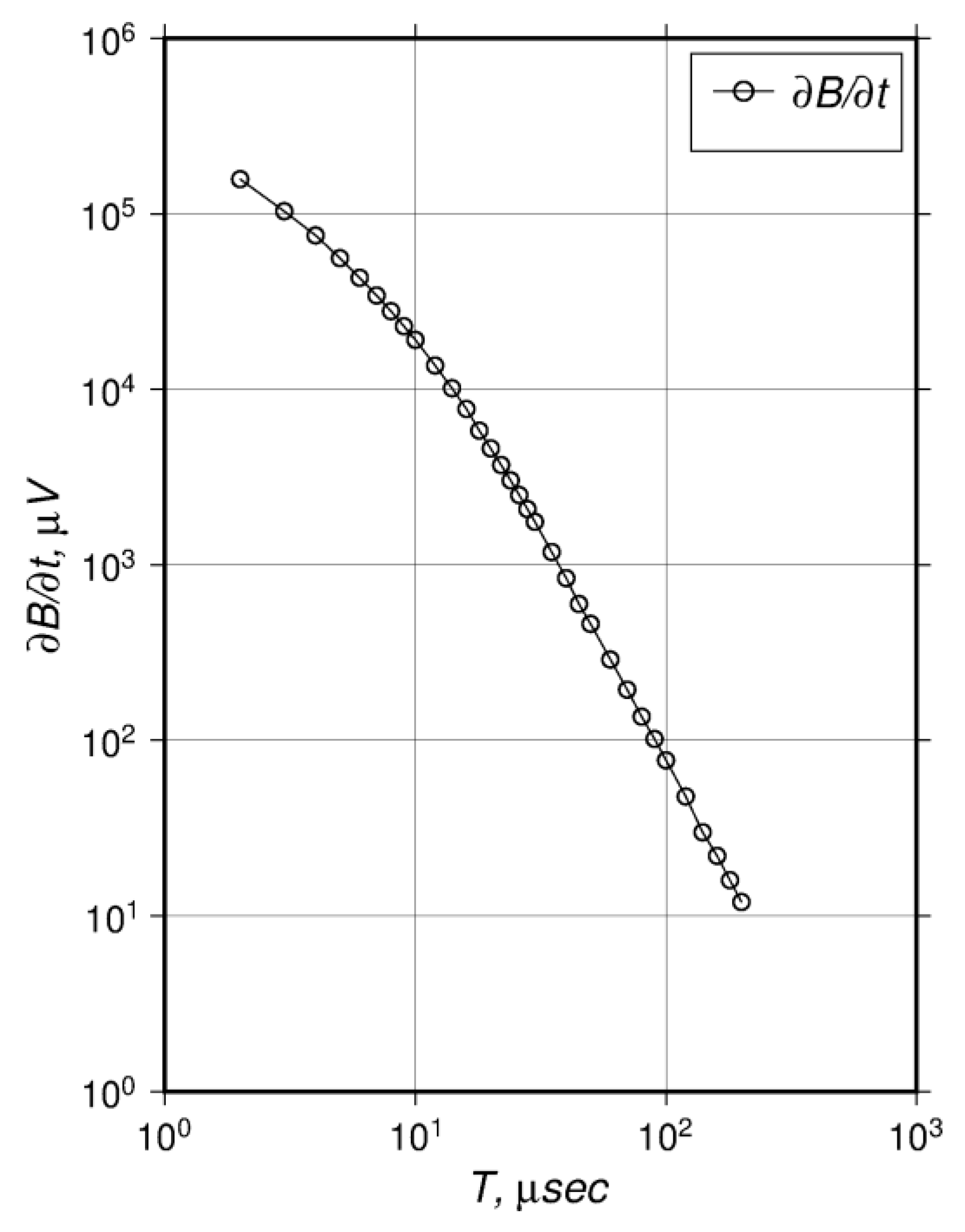
The measured voltage as a function of time (Equation (3)) after a steady current (square wave form) is abruptly turned off in the source loop at time t = 0, is used as experimental data for the TEM method, and is called the decay curve.

The decay curve is typically plotted on a bi-logarithmic scale (Figure 1).

3. Construction of Model

There are several techniques (also known as transformations) that are typically applied for determination of the approximate 1D distribution of the underground resistivity on the basis of experimental TEM data. The most widely used approach to the central loop TEM data is based on a moving thin sheet approximation of conductive half-space also known as S-inversion [22]. An actual inhomogeneous half-space at time t is characterized by an apparent surface conductance of an effective layer with a thickness approximately equal to the effective skin-depth. This layer is replaced by a conductive sheet of zero thickness with the apparent conductance S_τ positioned at the effective depth h_τ. For such a thin sheet model and for the late transient time, the value of S_τ can be found analytically [19,20,21]:

$$V_t=\frac{3IQq}{16\mathsf{\pi }{S}_{\tau }}\frac{1}{{\left(h_{\tau }+t/{\mu }_0{S}_{\tau }\right)}^4}$$

(4)

The values of interest S_τ and h_τ cannot be resolved simultaneously from Equation (4) for a certain time delay t. Several approaches exist to resolve this problem, however the so-called “differential” [23], based on the ratio of the measured signal to its first time derivative, is quite common. In this case the apparent conductivity of the thin sheet corresponding to the time delay t can be written as:

$$S_{\tau }=16{\left(\frac{\mathsf{\pi }}{3IQq}\right)}^{1/3}\frac{1}{{\mu }_0{}^{4/3}}\cdot \frac{{\left|V_t\right|}^{5/3}}{{\left({V^{\prime }}_t\right)}^{4/3}}$$

(5)

where ${V^{\prime }}_t$ is the first time derivative of the measured voltage, which can be calculated as a first difference from the decay curve (Equation (3)).

Having the values of the apparent conductivity and the effective depth from the simultaneous solution of Equations (4) and (5) and plotting them as S_τ(h_τ) for the same time delay t, the approximate 1D resistivity distribution can be calculated from such a plot as a relation of first differences (Figure 2):

$$\rho (h)=\mathsf{\Delta }h/\mathsf{\Delta }S.$$

(6)

The 1D model’s parameters (i.e., the layer’s thickness and resistivity) can be calculated based on the formal dependence of resistivity with the depth (Equation (3)) which is the result of the transformation.

The idea of the algorithm is as follows. Since the ρ(h) curve (Figure 2) is more or less a weighted averaging of true resistivity, we can suppose that the true resistivity of the layer has to be closer to the curve’s extrema (max/min), so for a crude approximation we have to find these values. The extrema can be easily found by finding the abscissa values where derivative of resistivity with respect to depth are equal to zero:

$$\frac{\partial \rho (h)}{\partial h}=0.$$

Exploiting the same idea, the thickness of layers can also be calculated. The inflection points of the resistivity curve ρ(h) relate to the zero values of the second derivative of this curve with respect to depth $\frac{{\partial }^2\rho }{\partial h^2}=0$. So, in such a way we can obtain the preliminary approximation of the 1D model’s parameters by finding the zeros of first and second derivative of the resistivity curve ρ(h) Equation (6).

The derivatives can be estimated in several ways. The simplest approach is the direct application of the finite difference formulas to the mentioned ρ(h) curve or by calculating some approximation function for which the derivatives can be easily calculated analytically. Since the noise level increases with time in the attenuating TEM signals and differentiation enhances it, we applied the piecewise spline approximation to the experimental curve ρ(h). In that case, the derivatives are obtained using polynomial coefficients, which are available for each node. We even omit calculation of the first derivative in our algorithm. See next section.

4. Step-by-Step Description of the Algorithm for Express Analysis

1. Loading and rescaling data. Time delay values T(i) have to be in seconds and the voltages induced in a receiver loop at certain time delay V(i) have to be in volts.

2. For further calculations, the log10(T(i)) and log10(V(i)) are used.

3. Since the experimental TEM data in our case have slightly irregular logarithmic steps, we calculate the new regularly spaced delay time grid with the step 0.05 in log10(T(i)), which corresponds to 20 values per order in time.

4. Interpolation of measured voltage decay values by cubic spline for the new regular time sequence based on the three independent experimental data sets, created by choosing every third value from the irregular experimental sequence and subsequently averaging them to obtain a single regularly spaced decay curve.

The nearby layers with different resistivity cause the decay curve slope to change, so such an approach to interpolation provides that the conductive layer of interest is detected by at least three measurements at subsequent delays, otherwise the data is treated as measurement noise and averaging will reduce the influence of such data on the resulting model.

5. The derivatives of the averaged decay curve are calculated for each regularly spaced time node based on the piecewise polynomial coefficients returned by the spline algorithm.

6. The experimental curve interpolated in such a way as well as the derivatives are used in the S-inversion algorithm. So, subsequent steps from 7 to 11 are repeated for each time delay i.

7. The experimental values of the auxiliary function φ(m) are calculated:

$${\phi }_i{(m)}_{\exp }=\frac{3\mathsf{\mu }Qq}{\mathsf{\pi } r^3}\frac{E_i{}^{\prime }}{E_i{}^2}.$$

This function φ(m) is based on asymptotic expressions for the transient process of the decaying electromagnetic field in the conducting halfspace, r is the side of the source loop, E_i = ΔV/I, and E_i’ = ΔV’/I.

8. The value m_i at which the experimental and the theoretical functions φ(m) coincide is found by a numerical minimization algorithm:

m_i = m, @ φ(m)_theor = φ(m)_exp.

The theoretical values of the function φ(m) are defined by the formula:

$${\varphi }_{}{(m)}_{theoret}=\frac{(3-96m^2+128m^4) {(1+4m^2)}^{5/2}}{m^2{(3-8m^2)}^2}.$$

9. The integral conductance is calculated using values of m_i:

$$S(i)=S_i=\frac{3Qq}{\mathsf{\pi } r^4}\frac{m_i(3-8m_i^2)}{{(1+4m_i^2)}^{7/2}}\frac{1}{E_i}.$$

10. The depth to the conductive thin sheet is calculated by the formula:

h_i = 0.75 m_i r.

11. Having the values of the apparent conductivity S(t) and the effective depth h(t) the approximate 1D resistivity distribution ρ(h) is calculated as a relation of first differences:

$$\frac{\partial h}{\partial S}\left(i\right)=\frac{h_i-h_{i-1}}{S_i-S_{i-1}}.$$

12. Calculating the spline coefficients for each node of the ρ(h) curve.

13. Calculating the second derivative of the ρ(h) curve.

14. Analyzing node by node, we find the abscissa value where the second derivative changes its sign.

15. The case when the three successive nodes are changing the sign of the second derivative to opposite is considered as measurement noise, and is not accounted as a layer boundary. Only the case when the sign of the second derivative changes after two or more successive nodes with the similar sign is considered as a layer boundary.

16. For each detected layer the maximum or minimum resistivity value is calculated depending on the sign of the second derivative. This approach allows us to omit the use of the first derivative.

17. Output of results.

The algorithm was realized in the GNU Octave programming language [24].

5. Results

The application of the developed algorithm is demonstrated on real experimental TEM data, which were acquired with the in-loop configuration. Single-turn square loops with side of 20 m × 20 m and 10 m × 10 m were used as transmitting and receiving loops, respectively. Recorded data is represented in

Table 1. Experimental transient electromagnetic (TEM) data.

T (μs)	V (μV/A)	T (μs)	V (μV/A)
2.00	157,650.0	28.00	2080.0
3.00	103,650.0	30.00	1760.0
4.00	75,500.0	35.00	1185.0
5.00	55,950.0	40.00	840.0
6.00	43,250.0	45.00	599.5
7.00	34,350.0	50.00	462.0
8.00	27,900.0	60.00	289.0
9.00	22,950.0	70.00	195.0
10.00	19,150.0	80.00	136.5
12.00	13,700.0	90.00	102.0
14.00	10,150.0	100.00	77.0
16.00	7750.0	120.00	48.0
18.00	5825.0	140.00	30.0
20.00	4610.0	160.00	22.0
22.00	3715.0	180.00	16.0
24.00	3030.0	200.00	12.0
26.00	2500.0

, where the first column is the time delay (in μs) from the beginning of the transient process and the second column is the electromotive force normalized on the current in the source loop (in μV/A) induced in the receiving loop. The appropriate experimental decay curve is plotted on a bi-logarithmic scale in Figure 1.

As a result of the application the developed algorithm to the experimental data (steps 1 to 11) we obtained the numerical array represented in

Table 2. Results of application the S-transformation to the experimental data.

T (μs)	V (μV)	h (m)	ρτ (ohm)
2.00	157,650.0000	6.3252	12.5688
3.00	103,650.0000	6.3545	8.4572
4.00	75,500.0000	6.4167	6.4676
5.00	55,950.0000	6.5825	5.4449
6.00	43,250.0000	6.7494	4.7705
7.00	34,350.0000	6.9232	4.3022
8.00	27,900.0000	7.0971	3.9560
9.00	22,950.0000	7.2829	3.7029
10.00	19,150.0000	7.4689	3.5050
12.00	13,700.0000	7.8586	3.2336
14.00	10,150.0000	8.2499	3.0546
16.00	7750.0000	8.6332	2.9269
18.00	5825.0000	9.1297	2.9095
20.00	4610.0000	9.5295	2.8529
22.00	3715.0000	9.9202	2.8106
24.00	3030.0000	10.3140	2.7850
26.00	2500.0000	10.7072	2.7705
28.00	2080.0000	11.1064	2.7680
30.00	1760.0000	11.4754	2.7580
35.00	1185.0000	12.4371	2.7768
40.00	840.0000	13.3414	2.7959
45.00	599.5000	14.3542	2.8769
50.00	462.0000	15.1162	2.8714
60.00	289.0000	16.6327	2.8970
70.00	195.0000	18.0137	2.9126
80.00	136.5000	19.4046	2.9573
90.00	102.0000	20.5604	2.9512
100.00	77.0000	21.8013	2.9864
120.00	48.0000	24.0163	3.0200
140.00	30.0000	26.6827	3.1953
160.00	22.0000	28.3008	3.1453
180.00	16.0000	30.2586	3.1960
200.00	12.0000	32.1546	3.2481

.

The appropriate resistivity curve as well as the 1D resistivity model which is the result of our algorithm (steps 12 to 17) are shown in Figure 2.

6. Discussions and Conclusions

The transformation mentioned above as well as other similar ones (e.g., [25]) yield qualitative information about geological cross-sections. For the effective interpretation of such results, additional information is required for referencing (i.e., wells logging data, geological information, results of other geophysical methods, etc.), and even the correlation of such TEM results from several neighboring sites allows the reliability to be improved. Therefore, simple approximate schemes for TEM data analysis have often been proposed [26,27].

The proposed rapid approach for determining the approximate 1D model of background conductivity, despite its simplicity, can be successfully applied in a number of practical cases. First, it can be applied at each field site right after taking the measurements to immediately assess the acquired data quality and crude comparison of the obtained resistivity cross section with the expected one, which can be known before as the additional geological information about the place under study, which allows optimization of the logistics of field works. Secondly, it can be used to construct 2D and/or 3D pseudo models, which will not be sufficiently precise, but main objects of interest should be highlighted so that the suspicious zones and places for further detailed study can be revealed without the involvement of time-consuming modeling and inversion algorithms. Finally, it can provide the initial 1D models for the further application of the EM inversions.

Obviously, the second and third conclusions have become less relevant recently because of the significant progress in computers as well as in computational algorithms. Even so, the simple models with between three and five layers are used as the starting model for the inversions [27]. However, in field conditions where the deployment of source and receiver loops consumes up to 90% of working time, the simple but reliable classical approach to express analysis is acceptable for supporting the decision undertaking to optimize the logistics of field works and quickly assess the danger state of geological medium.

The proposed method can be used for big data approaches and allows parallelization [9]. Thanks to the time series approach [11], the proposed method can also be used for other artificial intelligence tasks.