Stochastic Neighbor Embedding Feature-Based Hyperspectral Image Classification Using 3D Convolutional Neural Network

Abstract

The ample amount of information from hyperspectral image (HSI) bands allows the non-destructive detection and recognition of earth objects. However, dimensionality reduction (DR) of hyperspectral images (HSI) is required before classification as the classifier may suffer from the curse of dimensionality. Therefore, dimensionality reduction plays a significant role in HSI data analysis (e.g., effective processing and seamless interpretation). In this article, a sophisticated technique established as t-Distributed Stochastic Neighbor Embedding (tSNE) following the dimension reduction along with a blended CNN was implemented to improve the visualization and characterization of HSI. In the procedure, first, we employed principal component analysis (PCA) to reduce the HSI dimensions and remove non-linear consistency features between the wavelengths to project them to a smaller scale. Then we proposed tSNE to preserve the local and global pixel relationships and check the HSI information visually and experimentally. Lastly, it yielded two-dimensional data, improving the visualization and classification accuracy compared to other standard dimensionality-reduction algorithms. Finally, we employed deep-learning-based CNN to classify the reduced and improved HSI intra- and inter-band relationship-feature vector. The evaluation performance of $95.21\%$ accuracy and $6.2\%$ test loss proved the superiority of the proposed model compared to other state-of-the-art DR reduction algorithms.

1. Introduction

Hyperspectral imaging (HSI) captures a very large number of wavelengths of information that are spectrally separated by a narrow spectral waveband (i.e., 10 nm). HSI is usually used for satellite-image and land-cover analysis [1]. Now it is also used in various applications such as medical image analysis and diagnosis [2], food quality identification [3], material property detection [4], cultural heritage digitalization [5], forensic analysis [6], forest analysis [7], etc. [8,9,10]. Many researchers have been working to develop HSI recognition systems [11]. They are still facing some problems, such as more than a hundred image bands with the high resolution being included in HSI the image, which is highly informative but requires large memory and needs more processing time. In addition, the large number of bands yielding high dimensionality [11] is the main reason for the Hughes effect, which also significantly reduces the classification accuracy performance, known as the curse of dimensionality. Moreover, it has an overfitting problem, a major problem in machine learning algorithms [12]. As the HSI dataset contains many features, it degrades the classification performance because of the overfitting problem. Some researchers have found that similar spectral properties may be included in HSI for different objects [13]. For instance, the components used for construction, parking garages, and rooftops are similar [14], which indicates that their spectral signatures are difficult to distinguish. Ren et al. proposed a feature-extraction (FE) and DR method to recognize the HSIs based on these considerations. Their main goal was to solve the problems by reducing the dimensions and implementing effective feature extraction [15]. Furthermore, they used linear-type FE for DR, but this fails in cases where the mean and covariance are not enough to define the example datasets. Many algorithms are used in the HSI domain, such as a DR; principle component analysis (PCA) also finds undesirable linear correlations between the variables or features. In addition, this algorithm may fail because of the inefficiency of the extracted features. Moreover, it cannot ensure how many principal components should be considered. Some researchers proposed linear discriminant analysis (LDA) to solve this problem [16]. The main problem of LDA is that it cannot interpret new features because the number of components must be set manually. Some researchers proposed singular value decomposition (SVD) algorithms to solve the LDA problems [17]. Although SVD has many advantages to solving the DR problem, it is not easy to understand the data-transformation mechanism. Some researchers proposed the independent component analysis (ICA) method to solve the above problem. However, the major problem of the method is that it is oblivious to isolate the features that only extract the initial signals from the measurements [18]. Lastly, some researchers proposed kernel PCA (KPCA) to solve the problem, but it requires a longer computation time.

Recently Mateen et al. have proposed the t-Distributed Stochastic Neighbor Embedding (tSNE) [19] dimensionality-reduction algorithm for better image visualization and classification. The philosophy behind reducing and visualizing the dimensionality is to attain successful data processing and be quickly assimilated by a human analyst. Inspired by this concept, we proposed an extended tSNE and deep learning algorithms to solve the FE and DR problems and increase the HSI domain’s performance accuracy. The major contributions of this study are given below.

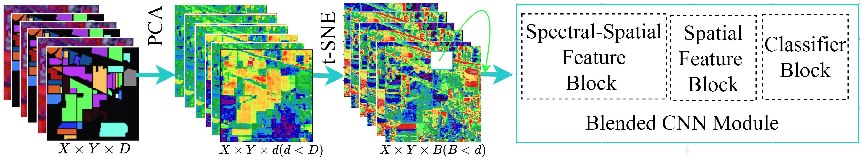
• We proposed a modified tSNE through the PCA algorithm to solve the visualization, dimensionality, and computational complexity problem. PCA is used to discover the irrelevant feature bands, aiming to increase the performance of tSNE. The tSNE preserves the intra- and inter-band relationship of the HSI, which is the most effective feature of the HSI for classification and visualization.
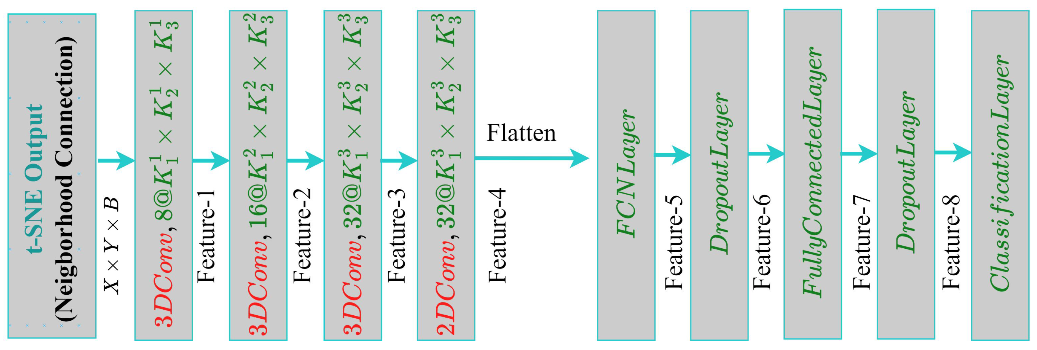
• We designed a new blended CNN architecture for feature extraction and classification, which is a sequential combination of 3D- and 2D-CNN to incorporate the spatial and spectral information of HSI, where the combined spectral information contains the wavelengths of the bands and the spatial information contains the location information of the band.
• Two benchmark HSI datasets were used to evaluate the proposed system, namely Indian Pines and SalinusA. Finally, the state-of-the-art comparison table proves the superiority of the proposed model over the mentioned systems.

We organized the study as a sequence with a literature review provided in Section 2. Section 3 demonstrates the different hyperspectral image datasets, although finally, we show the performance accuracy for only one dataset. The proposed methodology and each part of the study are described in Section 4. The evaluation performance is demonstrated in Section 5. Finally, the conclusions and future work are described in the Section 6.

2. Related Work

Many researchers have been working to develop hyperspectral image classification using various methodologies. Most researchers followed two steps: (i) hand-crafted feature extraction and the (ii) classification. Many researchers used an artificial neural network, k-nearest neighbour, parallelized maximum likelihood, logistic regression, or maximum distance classification algorithm to extract the efficient features from the hyperspectral images [20]. Zhong et al. employed an iterative SVM to classify hyperspectral images. They mainly extracted the principal components from the original image. They concatenated them with the original image to make the data cube fed to the SVM to produce the initial classification map. In addition, a Gaussian-filter map was employed to yield the spatial information from the previous map [21]. The existing methods use only spatial information, though many researchers think that spatial–spectral information is more effective than only spatial information. Shambulinga et al. employed SVM along with PCA and a guided image filter to classify hyperspectral images and achieved a good performance with a radial basis kernel (RBF) [22]. Later, they used LDA to reduce the dimensionality of the hyperspectral images [23,24,25]. Recently, researchers have focused on deep learning algorithms, which show efficiency in various domains such as vision [26,27,28,29,30] and NLP. Researchers have developed hyperspectral image classification to identify the efficiency of the various levels of the features. The deep-learning-based CNN model was trained with various levels of feature dimensions and used to identify the real artefact of the hyperspectral images [31,32]. Aydemir et al. employed deep learning approaches to classify hyperspectral images, using individual deep learning for each sensor [33]. In addition, they employed three kinds of clustering to solve the unlabeled problem: subtractive, modified k-means, and mean-shift clustering. They also exploited the labeled and unlabeled samples. Bidari et al. also employed a deep learning algorithm to classify hyperspectral images [34]. In addition, more recently, many researchers have proposed deep learning, including some dimension reduction to improve the efficiency of the hyperspectral-image-classification model [31,35,36,37,38,39,40]. Liu et al. applied a deep learning approach to classify and reconstruct hyperspectral images using MDL40w and achieved a 94.00% performance [41]. Yang et al. employed deep learning algorithms based on spatial and spectral correlations for enhancing the hyperspectral image classification [42]. They mainly employed four deep learning models, namely, 2D-CNN, 3D-CNN, recurrent 2D-CNN, and recurrent 3D-CNN, for classification and achieved a good performance accuracy. Although the existing method achieved a good performance, their computational complexity was great because of the high dimensionality. To solve this challenge, we propose PCA to reduce the dimensionality and then tSNE to calculate the relationship among the bands. Finally, we apply BlendedCNN to extract the final feature and classification purpose.

3. Dataset

In this work, two publicly available benchmark datasets (Indian Pines and SalinusA) were used. The datasets’ descriptions are given below. Among the various types of sensors, both of the examined image sets were collected using NASA AVIRIS sensors.

Table 1. Description of hyperspectral sensors.

Sensors	Organization	No. of Bands	Wavelength Range ($\mathsf{\mu }$m)
AVIRIS	NASA	224	0.40–2.50
AISA	Spectral Imaging Ltd.	286	0.45–0.90
CASI	Itres Research	288	0.43–0.87
PROBE-1	Earth Search Science Inc.	128	0.40–2.45

describes the various hyperspectral sensors. These data can be dwonloaded from the following link: https://www.ehu.eus/ccwintco/index.php/Hyperspectral_Remote_Sensing_Scenes (accessed on 1 April 2023).

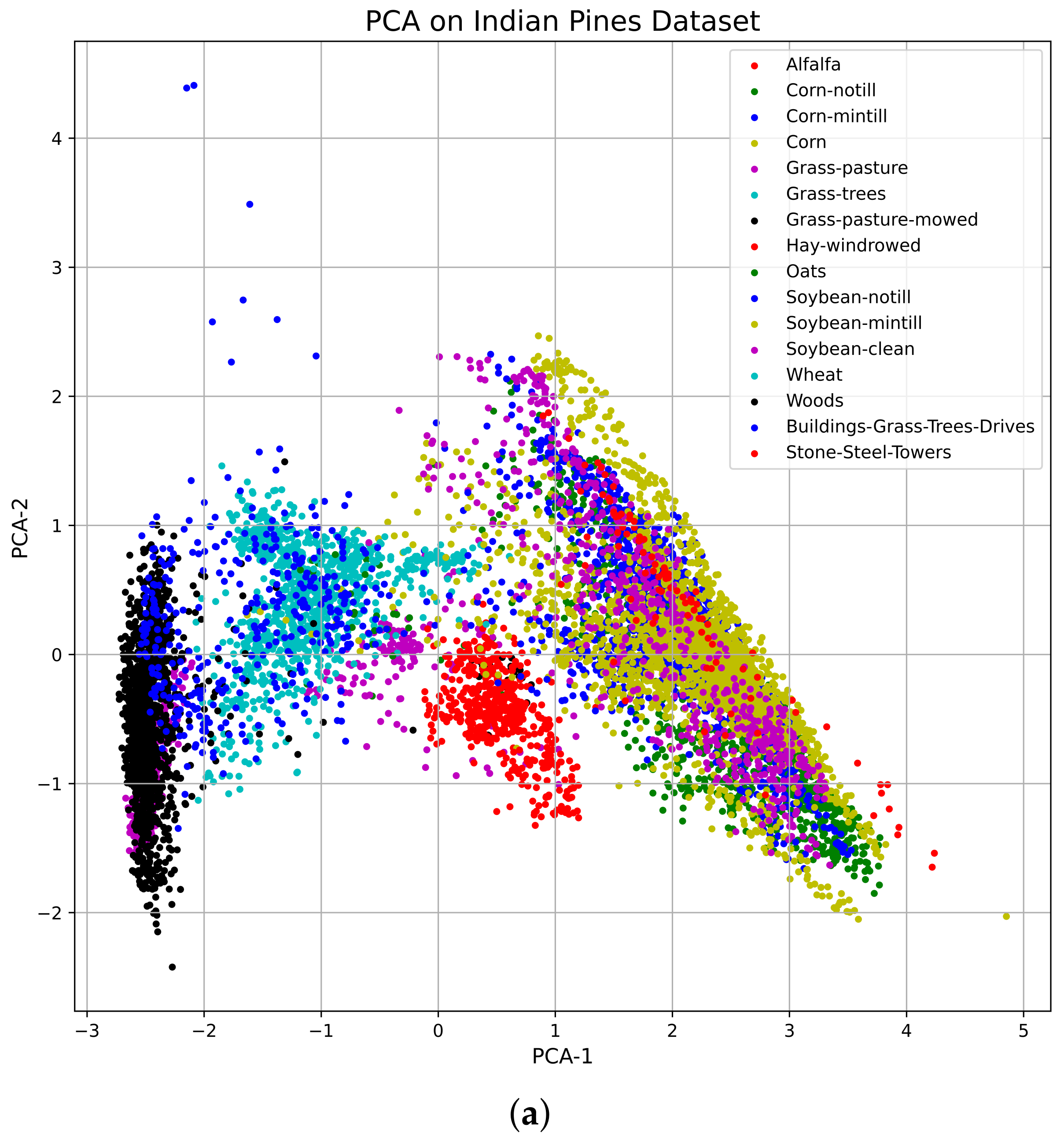
3.1. Indian Pines

The Indian Pines dataset was captured by NASA using Airborne Visible/Infrared Imaging Spectrometers (AVIRIS). The AVIRIS sensor uses a spectral range from $0.2$ to $2.4$ $\mathsf{\mu }$m, generating 224 unique bands. The number of collected bands was attenuated to 200 by eradicating 20 water-suction bands for the experiment. The spatial resolution of the images is 20 m per pixel, and the pixel size is $145\times 145$. For the experimental setup, it was downsampled to $73\times 73$ pixels, and the number of bands was 200. Indian Pines comprises 16 ground-truth classes containing different types of crops (e.g., corn, soybeans, and wheat) [43]. Figure 1 pictorially shows the dataset with a false-color composite image, ground-truth image, and corresponding class labels.

3.2. Salinas

The NASA AVIRIS sensor also collects the Salinas image set at Salinas Valley, California. The Salinas image dataset also contains 224 spectral bands. The size of each band is $512\times 217$ pixels. During the preprocessing for the experiment, 20 water-contaminated bands were reduced. The Salinas dataset contains classes of 16 ground-truth objects illustrating vegetables, bare soils, and vineyard fields. The collected image has been downsampled to $83\times 86$ with 200 bands. 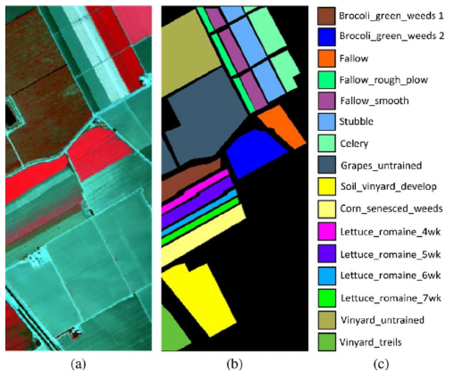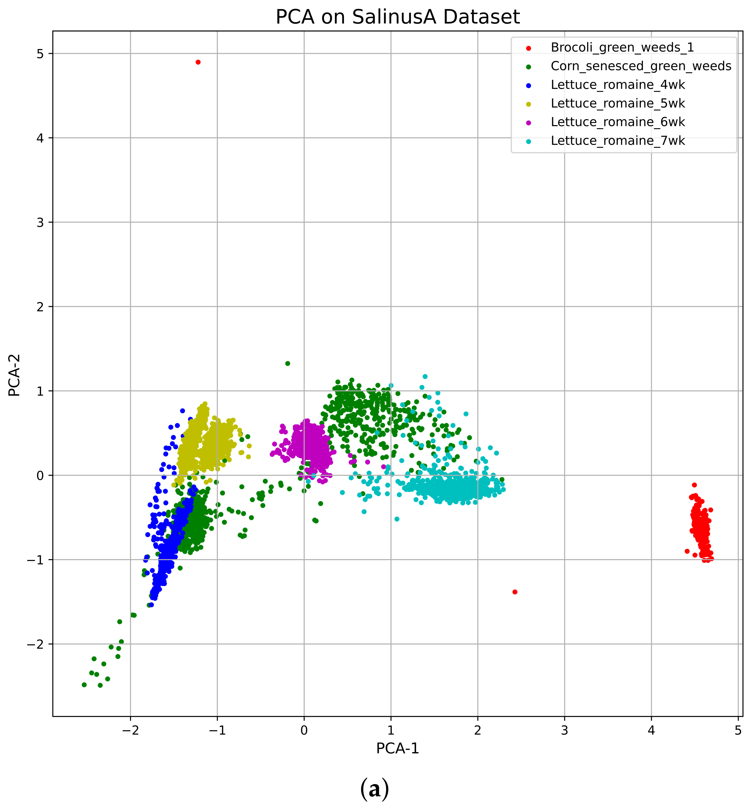Figure 2 illustrates the dataset with a false-color composite image and ground-truth image with the corresponding class labels.

4. Proposed Methodology

There are several advantages to the huge number of image bands in hyperspectral images; this high dimensionality is one of the biggest challenges to deal with while processing [44]. Although many existing studies deal with the high-dimensional bands with PCA or a similar solo method, we focus here on a multistage dimension-reduction method that makes our model different and unique from others. In our study, we first scaled in the preprocessing stage with a min–max scalar model. Then the standardized image is given as input for the feature extraction, dimension-reduction method, and classification. The whole process of the proposed study can be divided into three parts. The first one is feature extraction and efficient feature selection. The second one is to calculate the inter-and intraclass relationship between the spectral bands with visualization. The third one is the classification module. Our working flow chart of the proposed model for hyperspectral images is shown in Figure 3. The algorithm of the proposed method is described in Algorithm 1.

Let a 3D hyperspectral data cube be used as input data that is denoted by $I\in R^{M\times N\times D}$; here, the original input image is defined by I; the width, height, and bands are denoted by M, N and D, respectively, of the HSI. D spectral bands are included in each HSI pixel I. Let the categories of the land be denoted by C. Then the formula of a one-hot label vector can be written as $Y=(y_1,y_2,\dots ,y_C)\in R^{1\times 1\times C}$. Although the land-cover classes are not always distinct in hyperspectral images, most of it can be mixed because of the large intraclass variability and low interclass similarity into I [43]. We proposed the tSNE algorithm to calculate the intra-and interclass relationship to reduce this problem. As we said, hyperspectral images contain a high-dimensional band, which can reduce the speed and efficiency of the tSNE approach. To reduce the dimensions first, we used conventional DR algorithm PCA to remove the spectral redundancy over the original hyperspectral data (I).

Algorithm 1 Proposed Method Pseudocode

Input: Set of Input Dataset $P_i\in P\left(n\right)$ with dimension $X\times Y\times D$

Number of Samples: N, 70% for Training and 30% for Test

Output: Set of predicted class $s_i$

$\mathbf{Dimension}\mathbf{Reduction}\leftarrow PCA(X\times Y\times D)$

$\mathbf{Inter}\mathbf{and}\mathbf{Intra}\mathbf{Class}\mathbf{Feature}\leftarrow tSNE(X\times Y\times d)$

define BlendedCNNModel(input=$X\times Y\times B$, outputs=ClassificationLayer):

$SpectralSpatialFeature\leftarrow Spectral-Spatial\left(input\right)$

$SpatialFeature\leftarrow Spatial-Feature\left(SpectralSpatialFeature\right)$

$PredictedClass\leftarrow Classifier\left(SpatialFeature\right)$

return PredictedClass

while $i\ne NumEpochs$ do

$\hspace{1em}$// For Training

while $Batch\ne NumberBatchTraining$ do

$\hspace{1em}\hspace{1em}PredictedClass\leftarrow Model\left(Batch\right)$

$\hspace{1em}\hspace{1em}Loss\leftarrow Criterion(PredictedClass,Trai{n}_{C}lass)$

$\hspace{1em}\hspace{1em}Updatetheloss\leftarrow Loss.backward\left(\right),Optimizer.Step\left(\right)$

// For Testing

while $Batch\ne NumberBatchTesting$ do

$\hspace{1em}\hspace{1em}PredictedClass\leftarrow Model\left(Batch\right)$

$\hspace{1em}\hspace{1em}Output\leftarrow CPerformanceMatrix(PredictedClass,TestClass)$

The dimensions of each section where PCA reduced the total count of spectral bands from D to d are shown in Figure 3. shows the dimension of each section where PCA decreases the number of spectral bands from D to d. After applying the tSNE on the reduced data, we got the new dimension d to B. Although spatial information kept their dimension unchanged in every stage, spectral dimension decreased in every stage which is very important to identify any earth objects from the hyperspectral image. After applying PCA and tSNE, we got the new feature vector which is also a data cube that can be written as $F_x\in R^{M\times N\times B}$, here the output feature is denoted by $F_x$ which is mainly come from the tSNE and PCA modification of original dataset X, in the same way width, height and band are denoted by M, N and B respectively. We fed the final feature vector into a 3D Blended Convolution Neural Network (BlendedCNN) Classifier for the classification.

4.1. Principle Component Analysis (PCA) for HSI

HSI is usually applied for a particular application that does not significantly affect all the bands. Moreover, if the number of bands and input features increase, the classifier can be impacted badly to achieve a good performance in such application areas [45]. To minimize these limitations and extract potential features from high-dimension spectral data, it is crucial to select potential bands from the high-dimensional bands [46]. The key goal of the band selection is to project the original hyperspectral data onto a lower-dimensional subspace to represent the data accurately. These feature-extraction methods can be linear or nonlinear.

PCA is a popular approach to extracting features from hyperspectral images because these data contain multiple spectral data bands. PCA can extract details about the object’s emission and reflection properties based on the scene. PCA analyzes the covariance matrix of these data and extracts the principle components, which produce some new variables that are the output of a linear combination of the original spectral bands. Although it produces multiple variations, there are some priorities among them. Based on the priority property, it retained the most effective and relevant information. In summary, we selected the dimension with the larger eigenvalues. The first principal component describes the major input variability, and the second identifies the next maximum variability [47].

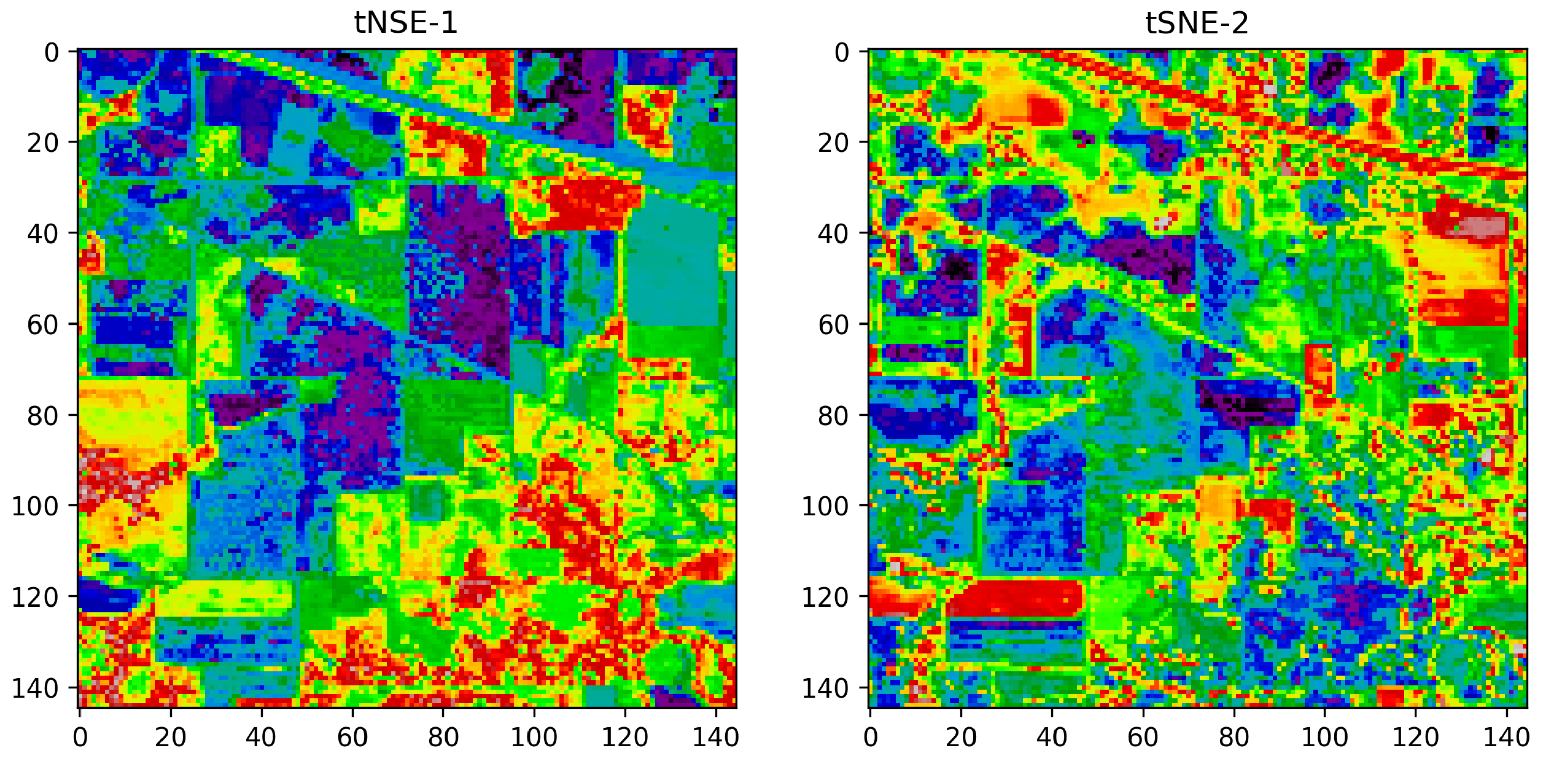
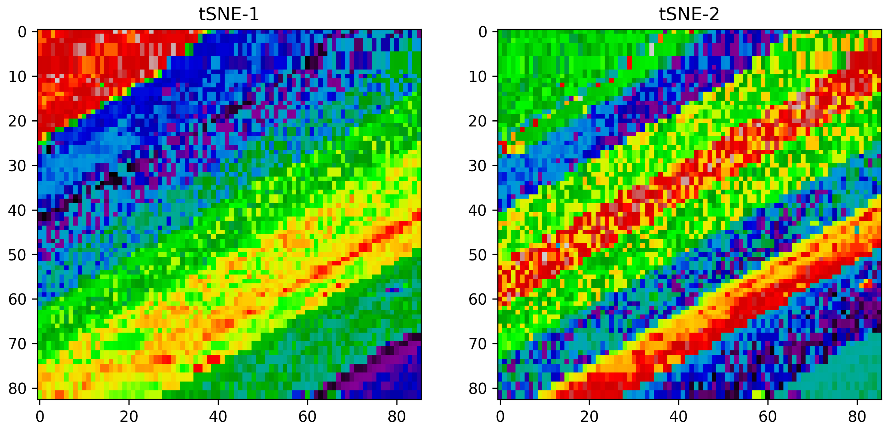
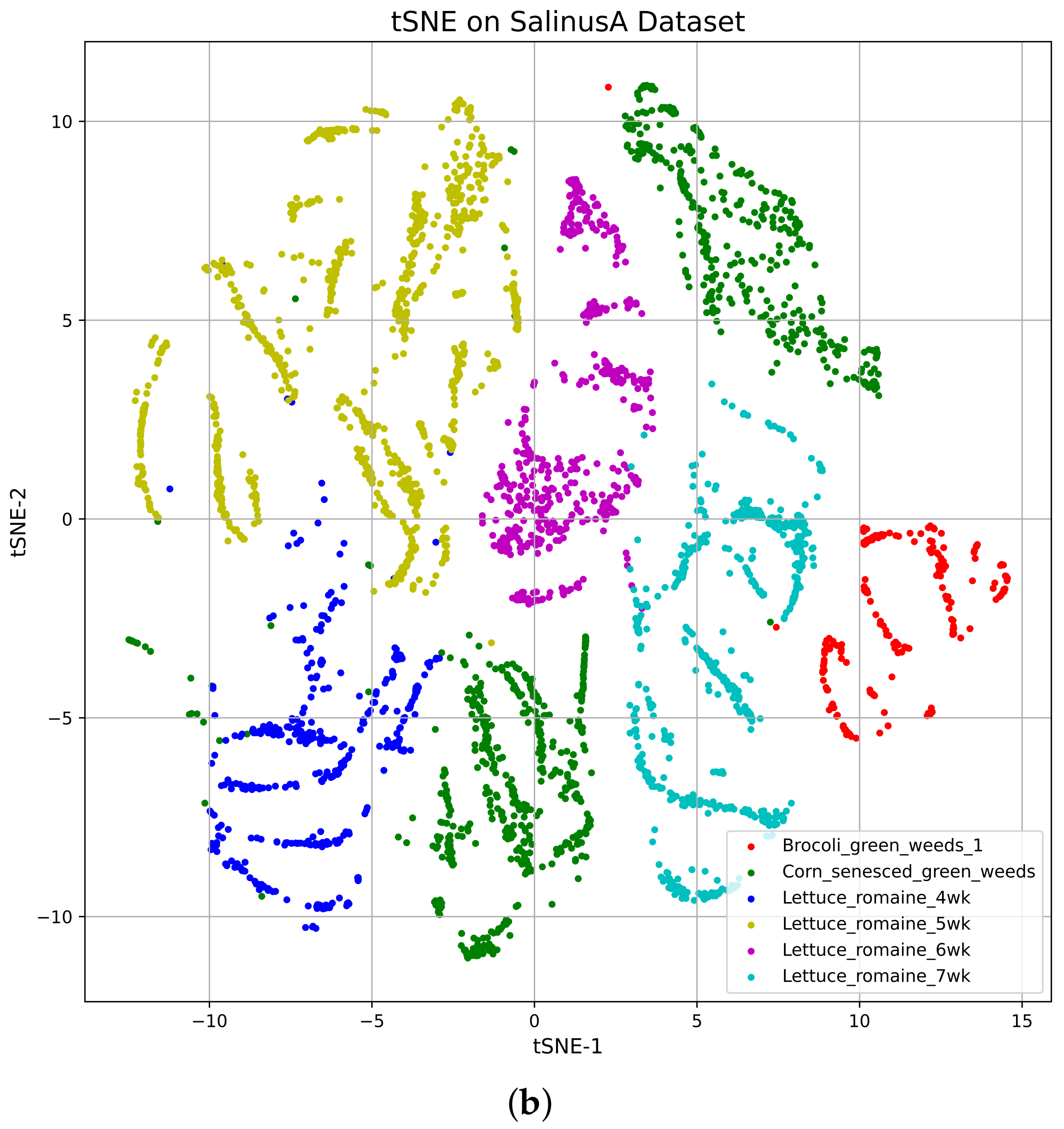
4.2. t-Distributed Stochastic Neighbor Embedding (tSNE)

We fed the reduced HSI potential feature to the tSNE to compute the inter- and intra- relationship among the spectral bands [19,48]. The main reason to use tSNE is the multidimensional scaling property and tremendous capacity to measure high-dimensional data to lower dimensions. The multidimensional scaling property and the enormous ability to reduce high-dimensional data to lower dimensions are the main reasons for using tSNE. The idea behind this algorithm is can be two-fold: The first stage is the Stochastic Neighbour Embedding (SNE) approach which is applied to the data points as an alternative projecting method of high dimensional Euclidean distance among the data point into a conditional probabilitie [19,48]. The conditional probability $P_{j|i}$ which is mainly express the relationship between two data points $x_j$ and $x_i$ can be described using the following Equation (1).

$$P_{j|i}=\frac{exp\frac{-{\parallel x_i-x_j\parallel }^2}{2{\sigma }_i^2}}{{\sum }_{i\ne k}exp\frac{-{\parallel x_i-x_k\parallel }^2}{2{\sigma }_i^2}}$$

(1)

Then, the probabilities are mathematically represented in the original feature space, just like in the following Equation (2).

$$P_{i,j}=\frac{(P_{i|j}+P_{j|i})}{2n}$$

(2)

where n is the dimension of the collection of results. The tSNE algorithm takes an input variable named "perplexity" and can be specified as a seamless calculation of an approximate number of neighbours [49]. Mathematically it can be expressed as

$$\begin{array}{c}\hfill Perp\left(P_i\right)=2^{H\left(P_i\right)}\end{array}$$

where $H\left(P_i\right)$ is the Shannon entropy, $P_i$ is measured in bits.

$$\begin{array}{c}\hfill H\left(P_i\right)=-\sum _j{P}_{j|i}{log}_2{P}_{j|i}\end{array}$$

This approach can dynamically adjust the variance ${\sigma }_i$ depending on the pairwise distance of the points to ensure the adequate number of neighbours overlaps with the user-provided perplexity [50]. To prevent traffic congestion the student t-distribution is used by tSNE with a specific degree of independence. The probability of low dimension $q_{ij}$ can be expressed quantitatively using another representation as in the following Equation (3).

This approach can dynamically adjust the variance ${\sigma }_i$ depending on the pairwise distance of the points to guarantee the active number of neighbours overlaps with the user-provided perplexity.

$$q_{ij}=\frac{{(1+{\parallel m_i-m_j\parallel }^2)}^{-1}}{{\sum }_{i\ne j}{(1+{\parallel m_i-m_j\parallel }^2)}^{-1}}$$

(3)

After that, the tSNE method finds the ways to project the input data $x_i$ into a lower dimension as $m_i$ look like as a Kullback–Leibler [51] approach by calculating the divergence between $p_{ij}$ and $q_{ij}$ and to achieved this tSNE employed a gradient-based approach. In tSNE, the parameters such as the number of components 2, verbose a, perplexity 40, and the number of iterations 300 have been used, which provide the best two components of the image.

Although tSNE better visualizes the data than PCA, there are still some disadvantages of tSNE; for example, it may take more time when the dataset is too large [19,48]. For this purpose, PCA is used for dimension reduction first, and then tSNE is applied to the reduced PCA features. Therefore, the processing time increases greatly. After that, the BlendedCNN, a deep convolutional neural network is applied to obtain a better classification accuracy, preserving both spatial–spectral relations of the HSI pixels.

Vizualization of the TSNE

The main goal of the tSNE is to preserve the local and global relationship between pixels. This tSNE algorithm provides a better-reduced dimension and better visualizes the data for linearly inseparable class data such as in the Indian Pines images. Figure 4 and Figure 5 the two main components after the tSNE algorithm for the Indian Pines and Salinas datasets, respectively. From this output, it can be shown that it provides the maximum information, like the ground-truth reference image.

The scatter plot of the outcome has been shown in Figure 6 and Figure 7 for Indian Pines and Salinas respectively. Figure illustrates the scatter plot for all classes of the Indian pines and SalinasA data set after dimension reduction using PCA and tSNE. Here it is clear that many classes are overlapped, and some classes are visually separated. A comparison discussion between PCS and tSNE is that many classes are clustered smoothly. Class Alfalfa in red color is more separated, and the Grass-pasture-mowed class in black colour is also separated from other classes. On the other hand, all other classes also show their separation from other classes. This statistical variation helps the improvement in the classification of the dataset.

4.3. BlendedCNN Architecture for HSI Classification

In this study, BlendedCNN—a spectral-spatial 3D-CNN accompanied by a spatial 2D-CNN—is utilized to classify hyperspectral images. BlendedCNN is a hybrid deep neural network that is created using a mixture of 3D and 2D CNN models and is intended for HSI image classification. The 3D-CNN model in this model maintains the spatial-spectral data from a set of spectral bands.

A 2D-CNN model is additionally introduced to the 3D-CNN in order to preserve and learn more about the spatial relationship between the HSI bands. In Figure 8, a visual representation of the network model is provided. This model primarily consists of three components: classification, 2D convolution of spatial information, and 3D convolution of spectral information. Our architecture began with a 3D convolution [52] to extract spectral data from HSI, which primarily convolved a 3D kernel with the 3D input tensor after which spectral feature of the convolution is formed by using the 3D kernel over various bands on the input layer.

The activation value $a_{m,n}^{p,q,r}$ at the $(p,q,r)$ for the $n^{th}$ feature map and at $m^{th}$ layer, calculated with the following equations.

$$a_{m,n}^{p,q,r}=\varphi (b_{m,n}+\sum _{\alpha =1}^{d_{l-1}}\sum _{\beta =-\zeta }^{\zeta }\sum _{\theta =-\gamma }^{\gamma }\sum _{\sigma =-\delta }^{\delta }{w}_{m,n,\alpha }^{\sigma ,\theta ,\beta }\times a_{m-1,\alpha }^{p+\sigma ,q+\theta ,r+\beta })$$

(4)

In the Equation (4), $2\zeta +1$ is the kernel depth along a spectral dimension, and other parameters are the same as in Equation (5).

In order to feed the 2D CNN with 2D data, the 3D data was first convolved with the 2D kernels. However, the convolution process is the same as the previous one by computing the sum of the dot product among the input data and kernel. In addition, here a stride is used, aiming to stride over the input data to extract the spatial dimension. After that, the feature from the convolution is fed into the activation function to perform the non-linearity property of the model. At the spatial position of the 2D convolution, the activation value is calculated according to the following equation.

$$a_{m,n}^{p,q}=\varphi (b_{m,n}+\sum _{\alpha =1}^{d_{l-1}}\sum _{\theta =-\gamma }^{\gamma }\sum _{\sigma =-\delta }^{\delta }{w}_{m,n,\tau }^{p,q},\times a_{m-1,\alpha }^{p+\sigma ,q+\theta })$$

(5)

where $(p,q)$ is the spatial position, $n^{th}$ is the feature index of the $m^{th}$ layer index, and the final feature is denoted by $a_{m,n}^{p,q}$. In addition, the activation function bias parameter is denoted by $\varphi$, $b_{m,n}$.

CNN parameters, such as the bias b and kernel weight w, can typically be trained with a gradient descent optimization method using supervised strategies [53]. In traditional 2D-CNNs, only spatial dimensions are added to measure the 2D discriminatory function maps, preserving all the image features of the prior layer. At the same time, the spectral information preserved in several bands and the spatial information can be obtained for the issue of HSI classification. The 2D-CNNs cannot manage the spectral results. Moreover, the 3D-CNN kernel can concurrently retrieve the spectral and spatial information from the input image data. To take advantage of the 2D- and 3D-CNNs’ automated feature-learning capability, a hybrid HSI classified feature-learning system called BlendedCNN is proposed. Figure 3 shows the data flow diagram of the BlendedCNN network. It consists of three 3D convolutions, one 2D convolution (Equation (4)), the other (Equation (5)), and three completely linked layers. Just before the flattening layer, the 2D convolution is implemented by considering that spatial information inside the various spectral bands is highly discriminated against without a serious decline of spectral information, which is essential for HSI details. It can be shown that the largest number of variables is found in the first dense layer. In the final layer, we used neurons, the same as the label of the Indian Pines dataset, which is 16.

In summary, the total sample dataset in the final layer depends on the number of classes in the dataset. For the Indian Pines dataset, the total number trainable parameters in our proposed network $5,122$, and 176. The backpropagation algorithm with Adam optimizer is used here to randomly initialize and train the model with a softmax loss function [54].

5. Experimental Setups and Results

In this work, we used the Indian Pines and SalinasA datasets, which contain 16 input classes each [43]. For all datasets, a dimension-reduction approach is applied first and takes the major dimensions of these datasets. Second, this research uses a BlendedCNN classification framework to train a classifier system that ensures that the properties of the system studied and trained on a common basis are passed and carefully designed to a new model for the target classes expected. The network used throughout the training methodology was explicitly configured with the metadata of the bounding boxes. To prevent the parameters learned from coevolutionary layers from pre-training, for the first stage of training, only the network head is trained independently with the training of hundreds of datasets of images. In contrast, all the foundation layers remain protected. Then, the training dataset tunes the global layers to form the BlendedCNN classification, which could benefit from the normalized features of large-scale data. In the training experiments, the batch size is 256 and the number of epoch is 100. The proposed classification model is implemented using the deep learning framework.

5.1. Experimental Settings

The image was first scaled in the preprocessing stage with a min–max scalar model. Then the standardized image was given as input for the dimension-reduction method. Here, tSNE was used as our DR algorithm. In tSNE, parameters including the number of components 2, verbose a, perplexity 40, and number of iterations 300 are used, which provide the best two components of the image. Then, this reduced dataset was split in a ratio of 70 and 30 as the training set and test set, respectively, for both input and ground-truth images. We used 256 as a batch size to obtain a stable model and trained the model for 100 iterations without batch normalization and data accumulation. After that, the output image was resized to prepare the image cube.

Then the image cube was used as input for the BlendedCNN model for classification, and the detailed information is given in

Table 2. Output dimension of the proposed BlendedCNN Model.

Layer (Type)	Output Shape	Parameter #
Input Layer	(None, 224, 224, 2, 1)	0
Conv3d Layer	(None, 25, 25, 2, 1)	0
Conv3d Layer	(None, 23, 23, 1, 8)	152
Conv3d Layer	(None, 21, 21, 1, 16)	1168
Conv2D Layer	(None, 19, 19, 64)	9280
Flatten Layer	(None, 23,104)	0
FCN Layer	(None, 256)	5,914,880
Dropout Layer	(None, 256)	0
Dense Layer	(None, 128)	32,896
Dropout Layer	(None, 128)	0
Output Layer	(None, 21, 21, 1, 16)

. The BlendedCNN model consists of one input layer, two $3D$ layers, one $2D$ layer, and one flattened layer, the sandwich combination of three dense and two dropout layers. Here the total and trainable parameter numbers are the same, and the value is $5,960,440$. For the non-trainable parameters, the number is 0. To implement the system, we used the Python programming language and Google colab.

To carryout the experiment We used the TensorFlow framework of Python programming [55] in the Google Colab environment with Pro edition. There are 25 GB RAM in the environment and a GPU named Tesla $P100$ [56]. Because it is open source, utilizes the idea of a computational graph, is adaptable, and works with the least amount of resources possible, Tensorflow is seen as a godsend to deep learning models. For the initial image processing task, we utilized the OpenCV Python library [57]. The image collection is also transformed into a byte stream for storage using the pickle package. For analyzing mathematical and statistical datasets, Pandas and Numpy are utilized, providing versatility when manipulating matrices. Plotting the various kinds of graph figures requires the usage of Matplotlib [57]. The training was performed for each dataset for 100 epochs while we used $0.000005$ as the initial learning rate on account of higher fluctuation during the Adam optimizer with Nesterov momentum [58,59]. Here different types of parameter tuning had been performed for the learning rate and optimization of two study classes.

5.2. Performance Accuracy with Indian Pines Dataset

The classification performance of the suggested technique using the Indian pines dataset is shown in

Table 3. Comparison of classification performance analysis for Indian Pines dataset [43].

	Recall	Precision	F1 Score	Test Loss	TA	KA	OA	AA	Time
SVD [43]	6	0	4	98	3.9	0	3.9	6.25	n/a
ICA [43]	85	92	94	27.23	94.16	93.37	94.2	85.12	n/a
NMF [43]	93	89	94	42.62	94.25	93.44	94.25	92.89	n/a
KPCA (Cosine) [43]	94	94	94	37.82	93.97	93.13	93.97	90.69	n/a
KPCA (RBF) [43]	85	87	85	96.82	85.49	83.35	85.49	81.36	n/a
MKPCA (Cosine + Linear) [43]	96	96	96	23.95	95.75	95.16	95.76	89.96	n/a
MKPCA (Cosine + RBF) [43]	95	95	94	23.75	94.53	93.75	94.53	90.73	n/a
SVM [60]	n/a	n/a	n/a	n/a	n/a	85.3	83.10	79.03	n/a
2D-CNN [61]	n/a	n/a	n/a	n/a	n/a	89.48	87.96	86.14	1.3
3D-CNN [62]	n/a	n/a	n/a	n/a	n/a	91.10	89.98	91.58	10.6
Proposed	95	99	97	6.2	98.21	98.10	98.34	95.21	4.42

. We compared the suggested method to other approaches, including Non-negative matrix factorization (NMF), Independent component analysis (ICA), Singular value decomposition (SVD), Kernel Principle Component Analysis (KPCA), and Multiple KPCA (MKPCA) with Cosine and RBF kernel, in order to demonstrate the effectiveness of the proposed approach. Figure 9 shows some classified images with the proposed and previous existing methods [43].

The classification accuracy performance is listed in Table 3, and it can be seen that SVD(Singular Value Decomposition) and BlendedCNN provide the least performance measures in all points of view. ICA and BlendedCNN provide moderate performance in all cases with $85.12\%$ Average Accuracy(AA). NMF and blended CNN algorithms provide $92.89\%$ of average accuracy, which is far better than SVD and ICA algorithms. Different kernels show different accuracy values compared to KPCA and MKPCA. Among them, the combination of Cosine and RBF in the kernel in MKPCA provides better average accuracy of $90.73\%$. On the other hand, the proposed tSNE and BlendedCNN show the best performance for the studied dataset, $95.21\%$, the highest among the studied methods. Thus, it can be concluded that tSNE with the BlendedCNN algorithm outperforms the studied baseline approaches. The tSNE algorithm provides quick saturation of the training accuracy in only 25 epochs with an accuracy of almost $100\%$. NMF provides near accuracy after 70 epochs. All others, i.e., KPCA with different kernels and ICA, are almost similar. However, SVD provides the lowest training accuracy. Therefore, it is easily shown that tSNE provides the best training accuracy on this example dataset. The testing accuracies of the studied methods are presented in Figure 10, and it can be seen that the testing accuracy of the proposed method is higher than that of all the baseline methods. It provides quick saturation in the accuracy after only 20 epochs with an accuracy of almost $98\%$. MKPCA with RBF and cosine kernel provides near accuracy after 95 epochs.

5.3. Performance Accuracy with SalinasA Dataset

The performance comparison of the proposed model with the state-of-the-art models for the SalinasA dataset is demonstrated in

Table 4. Comparison classification performance analysis for SalinasA dataset [31].

Method Name	Training Accuracy	Testing Accuracy	Time (s)
SVM [60]	N/A	92.95	N/A
2D-CNN [61]	N/A	97.08	2.0
3D-CNN [62]	N/A	93.96	15.2
HybridSN [31]	N/A	99.71	9.00
Proposed	99.99	99.96	5.63

. The output of the Salinas dataset after applying tSNE given on Figure 5. The Figure 7 visualizes the scatter plot of the clusters of different classes after PCA and tSNE applied. The Figure 11 illustrate the classification map or prediction of the proposed model using the SalinasA dataset. The visualization image Figure 11a,b seem to be the same because of the prediction performance near the 100%, and it showed the same as the original or ground truth images.

In the Table 4, we have shown the comparison of the proposed study with the most widely used method, namely SVM [60], 2D-CNN [61], 3D-CNN [62] and HybridSN method [31]. The training and testing data ratio is the same as in the previous study of Indian pines. The Table 4 conclude that the proposed model outperformed the existing method for the SalinasA dataset. In the same way, the classification map of the proposed method is better than the existing method also, the small segment maps also higher than the existing system.

6. Conclusions

In this research, the performance of the different DR algorithms is compared with the proposed tSNE after PCA and BlendedCNN method. It can be seen that the proposed method outperforms the baseline methods on real hyperspectral datasets. Various classification performance analysis terms, such as the test loss rate, over accuracy (OA), average accuracy (AA), precision, recall, and F1 score, are also shown. From the above analysis, it can be concluded that the proposed method can provide a better separation among the input classes of interest and address the curse of dimensionality issues. The tSNE preserves the local and global relationship of the pixel values, and PCA provides reduced-dimensional data. BlendedCNN preserves the spatial and spectral information of the reduced dataset for better classification of hyperspectral images. The main limitation of this work is that we used a multistage dimension-reduction method, which seems not to be smart, although it decreased the computational complexity of the system. In the future, we will extend the proposed deep learning model with different modalities such as spatial attention, temporal attention, spectral attention, dilated convolution, etc. and limit the learnable parameters in the explainable number without compromising the computational complexity, efficiency, and performance.

References

- Lebedev, A.; Zavarzin, V.; Gemonov, A. Vegetation Cover Change in Kologrivsky Forest Nature Reserve Detected using Landsat Satellite Image Analysis. IOP Conf. Ser. Earth Environ. Sci. 2020, 507, 012016. [Google Scholar] [CrossRef]
- Fei, B. Chapter 3.6—Hyperspectral imaging in medical applications. In Data Handling in Science and Technology; Amigo, J.M., Ed.; Elsevier: Amsterdam, The Netherlands, 2020; Volume 32, pp. 523–565. [Google Scholar] [CrossRef]
- Contributors. In Hyperspectral Imaging for Food Quality Analysis and Control; Sun, D.W., Ed.; Academic Press: San Diego, CA, USA, 2010; pp. 9–11. [CrossRef]
- Ziemann, A.; Theiler, J. Material Detection in Hyperspectral Imagery in Support of Nuclear Nonproliferation. 2016. Available online: https://public.lanl.gov/jt/Papers/Ziemann_Theiler_ANS2016_v2.pdf (accessed on 1 January 2023).
- Bai, D.; Messinger, D.W.; Howell, D. A pigment analysis tool for hyperspectral images of cultural heritage artifacts. In Proceedings of the Algorithms and Technologies for Multispectral, Hyperspectral, and Ultraspectral Imagery XXIII, Anaheim, CA, USA, 11–13 April 2017; Velez-Reyes, M., Messinger, D.W., Eds.; International Society for Optics and Photonics, SPIE: Bellingham, WA, USA, 2017; Volume 10198, pp. 429–443. [Google Scholar] [CrossRef]
- Edelman, G.; Gaston, E.; van Leeuwen, T.; Cullen, P.; Aalders, M. Hyperspectral Imaging for Non-Contact Analysis of Forensic Traces. Forensic Sci. Int. 2012, 223, 28–39. [Google Scholar] [CrossRef] [PubMed]
- Kibria, K.A.; Chowdhury, A.A.; Miah, A.S.M.; Shahriar, M.R.; Pervin, S.; Shin, J.; Rashid, M.M.; Sarkar, A.R. Bangladeshi Land Cover Change Detection with Satelite Image Using GIS Techniques. In Machine Intelligence and Data Science Applications: Proceedings of MIDAS 2021, Cumilla, Bangladesh, 26–27 December 2021; Springer: Berlin/Heidelberg, Germany, 2022; pp. 125–143. [Google Scholar]
- Mukundan, A.; Tsao, Y.M.; Cheng, W.M.; Lin, F.C.; Wang, H.C. Automatic Counterfeit Currency Detection Using a Novel Snapshot Hyperspectral Imaging Algorithm. Sensors 2023, 23, 2026. [Google Scholar] [CrossRef] [PubMed]
- Huang, H.Y.; Hsiao, Y.P.; Mukundan, A.; Tsao, Y.M.; Chang, W.Y.; Wang, H.C. Classification of Skin Cancer Using Novel Hyperspectral Imaging Engineering via YOLOv5. J. Clin. Med. 2023, 12, 1134. [Google Scholar] [CrossRef] [PubMed]
- Mukundan, A.; Huang, C.C.; Men, T.C.; Lin, F.C.; Wang, H.C. Air Pollution Detection Using a Novel Snap-Shot Hyperspectral Imaging Technique. Sensors 2022, 22, 6231. [Google Scholar] [CrossRef]
- Chang, C. Hyperspectral Data Processing: Algorithm Design and Analysis; John Wiley & Sons: New York, NY, USA, 2013. [Google Scholar] [CrossRef]
- Bu, C.; Zhang, Z. Research on Overfitting Problem and Correction in Machine Learning. J. Phys. Conf. Ser. 2020, 1693, 012100. [Google Scholar] [CrossRef]
- Zhao, W.; Du, S. Spectral–spatial feature extraction for hyperspectral image classification: A dimension reduction and deep learning approach. IEEE Trans. Geosci. Remote Sens. 2016, 54, 4544–4554. [Google Scholar] [CrossRef]
- Momeni, R.; Aplin, P.; Boyd, D. Mapping Complex Urban Land Cover from Spaceborne Imagery: The Influence of Spatial Resolution, Spectral Band Set and Classification Approach. Remote Sens. 2016, 8, 88. [Google Scholar] [CrossRef]
- Ren, J.; Zabalza, J.; Marshall, S.; Zheng, J. Effective Feature Extraction and Data Reduction in Remote Sensing Using Hyperspectral Imaging. Signal Process. Mag. 2014, 31, 149–154. [Google Scholar] [CrossRef]
- Bandos, T.V.; Bruzzone, L.; Camps-Valls, G. Classification of Hyperspectral Images with Regularized Linear Discriminant Analysis. IEEE Trans. Geosci. Remote Sens. 2009, 47, 862–873. [Google Scholar] [CrossRef]
- Menon, V.; Du, Q.; Fowler, J.E. Fast SVD with Random Hadamard Projection for Hyperspectral Dimensionality Reduction. IEEE Geosci. Remote Sens. Lett. 2016, 13, 1275–1279. [Google Scholar] [CrossRef]
- Falco, N.; Benediktsson, J.A.; Bruzzone, L. Spectral and Spatial Classification of Hyperspectral Images Based on ICA and Reduced Morphological Attribute Profiles. IEEE Trans. Geosci. Remote Sens. 2015, 53, 6223–6240. [Google Scholar] [CrossRef]
- Maaten, L.V.D.; Hinton, G.E. Visualizing Data using t-SNE. J. Mach. Learn. Res. 2008, 9, 2579–2605. [Google Scholar]
- Shambulinga, M.; Sadashivappa, G. Hyperspectral Image Classification using Convolutional Neural Networks. Int. J. Adv. Comput. Sci. Appl. 2021, 12, 702–708. [Google Scholar]
- Zhong, S.; Chang, C.I.; Zhang, Y. Iterative support vector machine for hyperspectral image classification. In Proceedings of the 2018 25th IEEE International Conference on Image Processing (ICIP), Athens, Greece, 7–10 October 2018; pp. 3309–3312. [Google Scholar]
- Shambulinga, M.; Sadashivappa, G. Hyperspectral Image Classification using Support Vector Machine with Guided Image Filter. Int. J. Adv. Comput. Sci. Appl. 2019, 10, 271–276. [Google Scholar] [CrossRef]
- Shambulinga, M.; Sadashivappa, G. Supervised Hyperspectral Image Classification using SVM and Linear Discriminant Analysis. Int. J. Adv. Comput. Sci. Appl. 2020, 11, 0111050. [Google Scholar] [CrossRef]
- Miah, A.S.M.; Rahim, M.A.; Shin, J. Motor-Imagery Classification Using Riemannian Geometry with Median Absolute Deviation. Electronics 2020, 9, 1584. [Google Scholar] [CrossRef]
- Miah, A.S.M.; Rashid, M.M.; Arahman, R.M.; Hossain, T.; Sujon, M.M.; Nafisa, N.; Mohammad, H.; Sin, J. Alzheimer’s Disease Detection Using CNN Based on Effective Dimensionality Reduction Approach. In Advances in Intelligent Systems and Computing, Proceedings of the 3rd International Conference on Intelligent Computing and Optimization 2020 (ICO 2020), Huai Khot, Thailand, 8–9 October 2020; Springer: Cham, Switzerland; Volume 1324, pp. 801–811.
- Miah, A.S.M.; Shin, J.; Hasan, M.A.M.; Rahim, M.A. BenSignNet: Bengali Sign Language Alphabet Recognition Using Concatenated Segmentation and Convolutional Neural Network. Appl. Sci. 2022, 12, 3933. [Google Scholar] [CrossRef]
- Miah, A.S.M.; Shin, J.; Hasan, M.A.M.; Rahim, M.A.; Okuyama, Y. Rotation, Translation and Scale Invariant Sign Word Recognition Using Deep Learning. Comput. Syst. Sci. Eng. 2023, 44, 2521–2536. [Google Scholar] [CrossRef]
- Shin, J.; Musa Miah, A.S.; Hasan, M.A.M.; Hirooka, K.; Suzuki, K.; Lee, H.S.; Jang, S.W. Korean Sign Language Recognition Using Transformer-Based Deep Neural Network. Appl. Sci. 2023, 13, 3029. [Google Scholar] [CrossRef]
- Miah, A.S.M.; Hasan, M.A.M.; Shin, J. Dynamic Hand Gesture Recognition using Multi-Branch Attention Based Graph and General Deep Learning Model. IEEE Access 2023, 11, 4703–4716. [Google Scholar] [CrossRef]
- Hasan, M.; Miah, A.S.M.; Hossain, M.M.; Hossain, M.S. LL-PMS8: A time efficient approach to solve planted motif search problem. J. King Saud Univ.-Comput. Inf. Sci. 2022, 34, 3843–3850. [Google Scholar] [CrossRef]
- Roy, S.K.; Krishna, G.; Dubey, S.R.; Chaudhuri, B.B. HybridSN: Exploring 3-D–2-D CNN feature hierarchy for hyperspectral image classification. IEEE Geosci. Remote Sens. Lett. 2019, 17, 277–281. [Google Scholar] [CrossRef]
- Wang, Y.; Ning, D.; Feng, S. A novel capsule network based on wide convolution and multi-scale convolution for fault diagnosis. Appl. Sci. 2020, 10, 3659. [Google Scholar] [CrossRef]
- Aydemir, M.S.; Bilgin, G. Semisupervised hyperspectral image classification using deep features. IEEE J. Sel. Top. Appl. Earth Obs. Remote. Sens. 2019, 12, 3615–3622. [Google Scholar] [CrossRef]
- Kumar, D.; Kumar, D. Hyperspectral Image Classification Using Deep Learning Models: A Review. J. Phys. Conf. Ser. 2021, 1950, 012087. [Google Scholar] [CrossRef]
- Devassy, B.M.; George, S. Dimensionality reduction and visualisation of hyperspectral ink data using t-SNE. Forensic Sci. Int. 2020, 311, 110194. [Google Scholar] [CrossRef]
- Luo, B.; Hussain, A.; Mahmud, M.; Tang, J. Advances in brain-inspired cognitive systems. Cogn. Comput. 2016, 8, 795–796. [Google Scholar]
- Fırat, H.; Asker, M.E.; Hanbay, D. Classification of hyperspectral remote sensing images using different dimension reduction methods with 3D/2D CNN. Remote. Sens. Appl. Soc. Environ. 2022, 25, 100694. [Google Scholar] [CrossRef]
- Ladi, S.K.; Panda, G.; Dash, R.; Ladi, P.K. A Pioneering Approach of Hyperspectral Image Classification Employing the Cooperative Efforts of 3D, 2D and Depthwise Separable-1D Convolutions. In Proceedings of the 2022 IEEE 2nd International Symposium on Sustainable Energy, Signal Processing and Cyber Security (iSSSC), Gunupur, India, 15–17 December 2022; pp. 1–6. [Google Scholar]
- Nayak, O.; Khandare, H.; Parida, N.K.; Giri, R.; Janghel, R.R.; Govil, H. Hyperspectral Image Classification using Hybrid Deep Convolutional Neural Network. Proc. J. Phys. Conf. Ser. 2022, 2273, 012028. [Google Scholar] [CrossRef]
- Butt, M.H.F.; Ayaz, H.; Ahmad, M.; Li, J.P.; Kuleev, R. A Fast and Compact Hybrid CNN for Hyperspectral Imaging-based Bloodstain Classification. In Proceedings of the 2022 IEEE Congress on Evolutionary Computation (CEC), Padua, Italy, 18–23 July 2022; pp. 1–8. [Google Scholar]
- Liu, S.; Shi, Q.; Zhang, L. Few-Shot Hyperspectral Image Classification with Unknown Classes Using Multitask Deep Learning. IEEE Trans. Geosci. Remote Sens. 2021, 59, 5085–5102. [Google Scholar] [CrossRef]
- Yang, X.; Ye, Y.; Li, X.; Lau, R.Y.K.; Zhang, X.; Huang, X. Hyperspectral Image Classification with Deep Learning Models. IEEE Trans. Geosci. Remote Sens. 2018, 56, 5408–5423. [Google Scholar] [CrossRef]
- Hossain, M.M.; Hossain, M.A. Feature Reduction and Classification of Hyperspectral Image Based on Multiple Kernel PCA and Deep Learning. In Proceedings of the 2019 IEEE International Conference on Robotics, Automation, Artificial-intelligence and Internet-of-Things (RAAICON), Dhaka, Bangladesh, 29 November–1 December 2019; pp. 141–144. [Google Scholar] [CrossRef]
- Hossain, M.M.; Hossain, M.A.; Al Mamun, M.; Hossain, M.M. Feature Reduction Based on the Fusion of Spectral and Spatial Transformation for Hyperspectral Image Classification. In Proceedings of the 2020 IEEE Region 10 Symposium (TENSYMP), Dhaka, Bangladesh, 5–7 June 2020; pp. 150–153. [Google Scholar] [CrossRef]
- Hughes, G. On the mean accuracy of statistical pattern recognizers. IEEE Trans. Inf. Theory 1968, 14, 55–63. [Google Scholar] [CrossRef]
- Jia, X.; Kuo, B.; Crawford, M.M. Feature Mining for Hyperspectral Image Classification. Proc. IEEE 2013, 101, 676–697. [Google Scholar] [CrossRef]
- Bartholomew, D.J. Principal Components Analysis. In International Encyclopedia of Education, 3rd ed.; Peterson, P., Baker, E., McGaw, B., Eds.; Elsevier: Oxford, UK, 2010; pp. 374–377. [Google Scholar] [CrossRef]
- Kabir, M.H.; Mahmood, S.; Al Shiam, A.; Musa Miah, A.S.; Shin, J.; Molla, M.K.I. Investigating Feature Selection Techniques to Enhance the Performance of EEG-Based Motor Imagery Tasks Classification. Mathematics 2023, 11, 1921. [Google Scholar] [CrossRef]
- García-Alonso, C.R.; Pérez-Naranjo, L.M.; Fernández-Caballero, J.C. Multiobjective evolutionary algorithms to identify highly autocorrelated areas: The case of spatial distribution in financially compromised farms. Ann. Oper. Res. 2014, 219, 187–202. [Google Scholar] [CrossRef]
- Gisbrecht, A.; Schulz, A.; Hammer, B. Parametric nonlinear dimensionality reduction using kernel t-SNE. Neurocomputing 2015, 147, 71–82. [Google Scholar] [CrossRef]
- Kingman, J.F.C. Information Theory and Statistics. By Solomon Kullback. Pp. 399. 28s. 6d. 1968. (Dover.). Math. Gaz. 1970, 54, 90. [Google Scholar] [CrossRef]
- Li, Y.; Zhang, H.; Shen, Q. Spectral-Spatial Classification of Hyperspectral Imagery with 3D Convolutional Neural Network. Remote Sens. 2017, 9, 67. [Google Scholar] [CrossRef]
- Miao, S.; Wang, J.Z.; Liao, R. Chapter 12-Convolutional Neural Networks for Robust and Real-Time 2-D/3-D Registration. In Deep Learning for Medical Image Analysis; Zhou, S.K., Greenspan, H., Shen, D., Eds.; Academic Press: Cambridge, MA, USA, 2017; pp. 271–296. [Google Scholar] [CrossRef]
- Zhang, Z. Improved Adam Optimizer for Deep Neural Networks. In Proceedings of the 2018 IEEE/ACM 26th International Symposium on Quality of Service (IWQoS), Banff, AB, Canada, 4–6 June 2018; pp. 1–2. [Google Scholar] [CrossRef]
- Abadi, M.; Agarwal, A.; Barham, P.; Brevdo, E.; Chen, Z.; Citro, C.; Corrado, G.S.; Davis, A.; Dean, J.; Devin, M.; et al. Tensorflow: Large-scale machine learning on heterogeneous distributed systems. arXiv 2016, arXiv:1603.04467. [Google Scholar]
- Tock, K. Google CoLaboratory as a platform for Python coding with students. Rtsre Proc. 2019, 2–1, 1–13. [Google Scholar]
- Gollapudi, S. OpenCV with Python. In Learn Computer Vision Using OpenCV; Springer: Berlin/Heidelberg, Germany, 2019; pp. 31–50. [Google Scholar]
- Glorot, X.; Bengio, Y. Understanding the difficulty of training deep feedforward neural networks. In Proceedings of the Thirteenth International Conference on Artificial Intelligence and Statistics, Sardinia, Italy, 13–15 May 2010; pp. 249–256. [Google Scholar]
- Dozat, T. Incorporating Nesterov momentum into Adam. In Proceedings of the Workshop given at International Conference on Learning Representation, San Juan, Puerto Rico, 2–4 May 2016. [Google Scholar]
- Melgani, F.; Bruzzone, L. Classification of hyperspectral remote sensing images with support vector machines. IEEE Trans. Geosci. Remote Sens. 2004, 42, 1778–1790. [Google Scholar] [CrossRef]
- Makantasis, K.; Karantzalos, K.; Doulamis, A.; Doulamis, N. Deep supervised learning for hyperspectral data classification through convolutional neural networks. In Proceedings of the 2015 IEEE International Geoscience and Remote Sensing Symposium (IGARSS), Milan, Italy, 26–31 July 2015; pp. 4959–4962. [Google Scholar]
- Hamida, A.B.; Benoit, A.; Lambert, P.; Amar, C.B. 3-D deep learning approach for remote sensing image classification. IEEE Trans. Geosci. Remote Sens. 2018, 56, 4420–4434. [Google Scholar] [CrossRef]