
Modelling of Electric Power Generation Plant Based on Gas Turbines with Agricultural Biomass Fuel

 , and
, and
Abstract
:1. Introduction
2. Materials and Methods
- Characterization of fuel based on agricultural biomass;
- References to model-based studies: thermodynamic, techno-economic, simulation, and mathematical;
- Description of mathematical models;
- Control system description;
- Matlab/Simulink simulation model of the whole system.
- Characterization of Biomass as fuel
- Power required: 1 kW
- 1 kW = 860 kcal/h, equivalence
- PCI: 4.384 (kcal/kg). Average value of the PCI of the coffee stem taken from Table 2
- 1 cal = 4.1855 kJ, equivalence
- B.
- References of studies based on different methods
- C.
- Description of the Mathematical Models
- Air and the products of combustion are considered ideal gases;
- The specific heats are considered constant for the products of combustion, air, and injected steam;
- The flow through the nozzles (compressor) is described as a polytropic, one-dimensional, and uniform adiabatic process;
- The energy storage and transport delay in the compressor, turbine, and combustion chamber are relatively small, which is why steady state equations are applied;
- The kinetic energy at the inlet of the gas flow in the compressor and turbine is considered negligible;
- The mass flow of air through the compressor is controllable by means of the blades at the inlet.
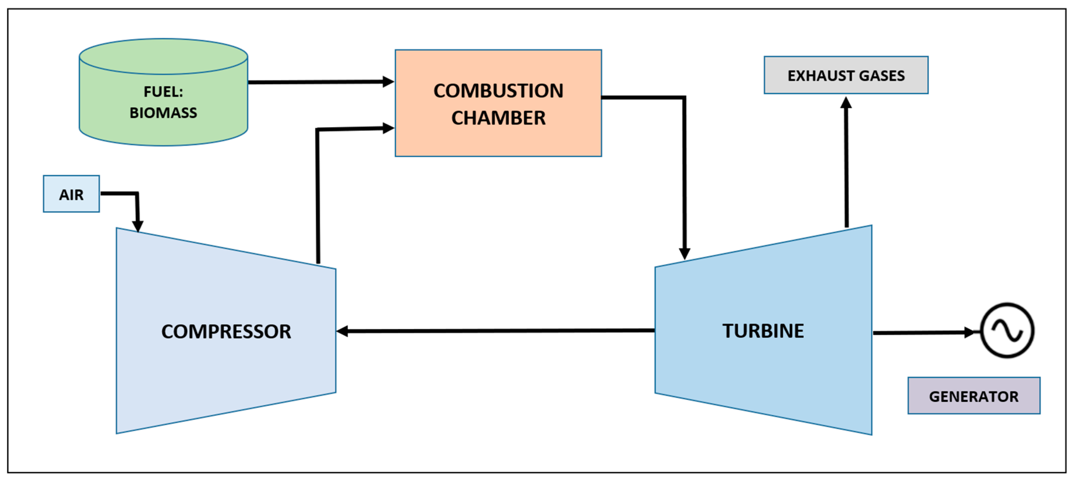
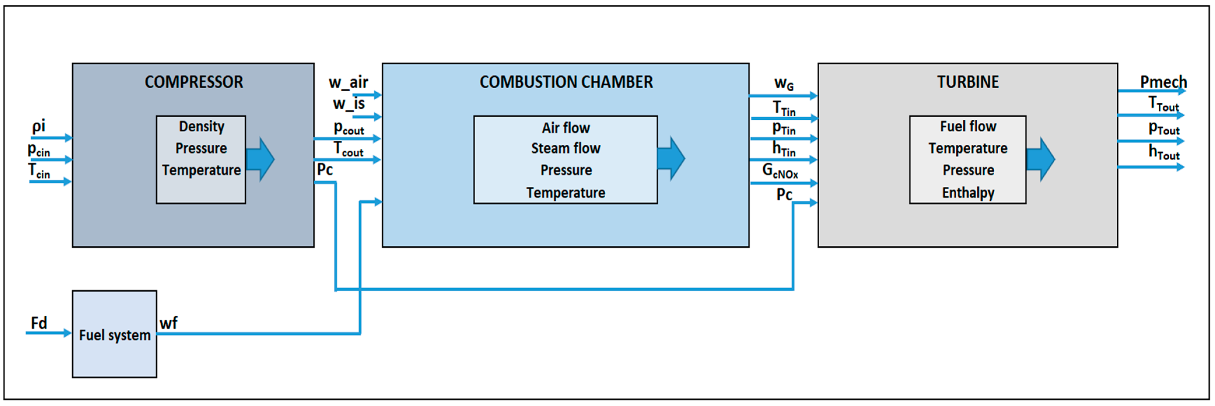
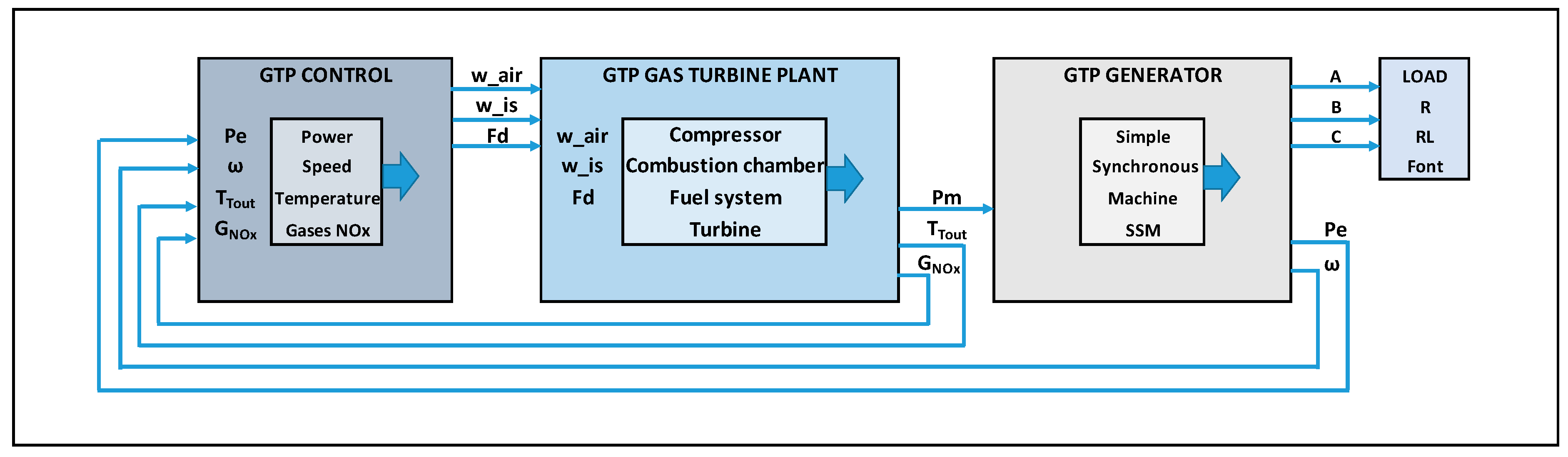
- Fuel system (valve with actuator)
- Compressor
- Combustion chamber
- Turbine
- Electric generator
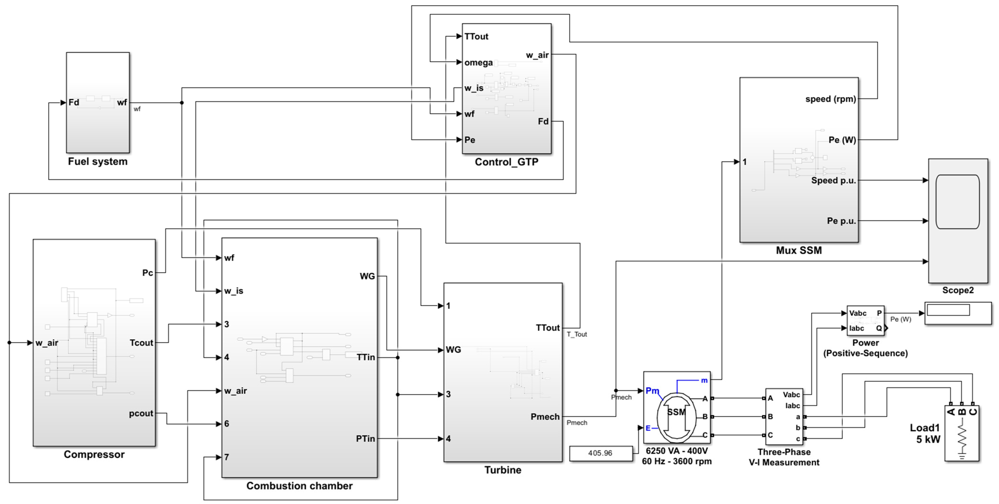
- Fuel System
- 2.
- Compressor
- 3.
- Combustion chamber
- 4.
- Turbine
- 5.
- Electric Generator
- D.
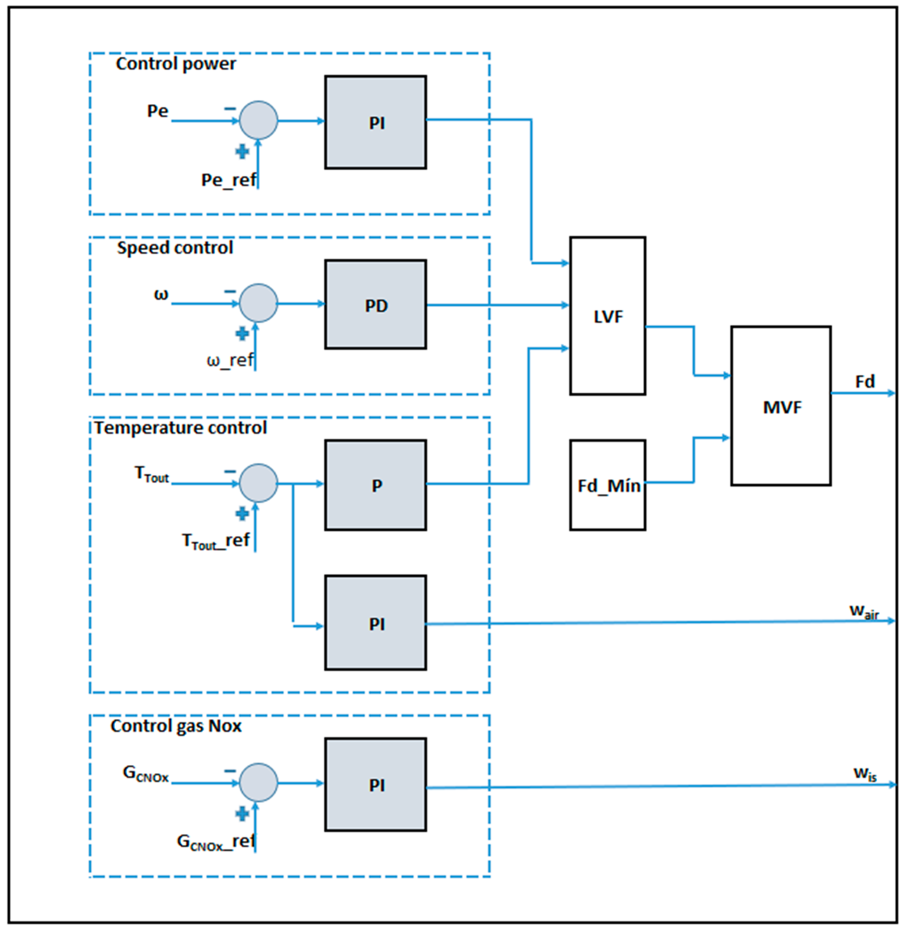
- Description of the control system
- Delivered mechanical power: Pmech, in W;
- Rotational speed (related to electrical frequency): ω in rad/s;
- Exhaust gas temperature: TTout in °K;
- Exhaust gas composition (NOx and CO content): gcNOx in p.p.m.
- Fuel flow: conversion of fuel quantity Fd to p.u.;
- Air flow (inlet guide vane position): wair in kg/s;
- Steam (or water) injection flow into the combustion chamber: wis in kg/s.
- Power control Pe: this is implemented with the electrical power signal Pe coming from the generator GTP (Gas Turbine Plant); this in turn receives the mechanical power signal Pmech coming from all of the dynamics of the GTP. This signal is subtracted from the reference signal Pe_ref, and the result of the subtraction is integrated in the PI controller generating the required dynamic power signal according to the requirements of the load and the dynamic behavior of the other signals;
- Speed control: similar to power control, the rotor speed signal ω comes from the GTP generator and performs a similar procedure; it is subtracted from a reference value ω_ref, and the result of the subtraction is derived in the PD controller generating the required dynamic speed signal according to the requirements of the load and the dynamic behavior of the other signals. This control must be considered in safety conditions so that the turbine does not lose balance and overspeed;
- Temperature Control TTout: the temperature signal comes from the Turbine block, and the temperature value is the highest of the compression and expansion process that occurs inside the plant; this parameter is important to control so that the temperature level does not exceed the upper temperature limit that the plant can withstand;
- Control of Outlet gases NOx: although a more robust and complex control of this block is not carried out, as it requires a deeper and more detailed development, it is important to take into account what it produces as a result in the outlet gases and pollutant components, as well as with the working temperatures; the behavior is reviewed as its process results in the steam flow of gases wis are the steam mass flow injection;
- LVF Block (Minimum Value Selector): this allows discrimination of the lowest value signal coming from the power, speed, and temperature controls, with the power signal predominating, without disregarding the other signals that are considered more for plant safety procedures, in terms of speed overflow and temperature level overshoot;
- MVF Block (Maximum Value Selector): this also complements the system, as it allows the higher signal of the two incoming signals to pass, which are the ones coming from the LVF block and Fd_Mín; this last block is very important as it provides the minimum flow signal that must be injected to the plant so that it does not shut down and maintains the flame of the combustion system.
- E.
- Matlab/Simulink simulation model of the whole system.
- GTP Control (Gas Turbine Plant);
- Fuel System;
- Compressor;
- Combustion Chamber;
- Gas Turbine;
- Simple Synchronous Machine (SSM);
- Simple Synchronous Machine (SSM) output multiplexer: speed in rpm, electrical power Pe (W);
- Three-phase outputs;
- Three-phase resistive load.
3. Discussion of Results
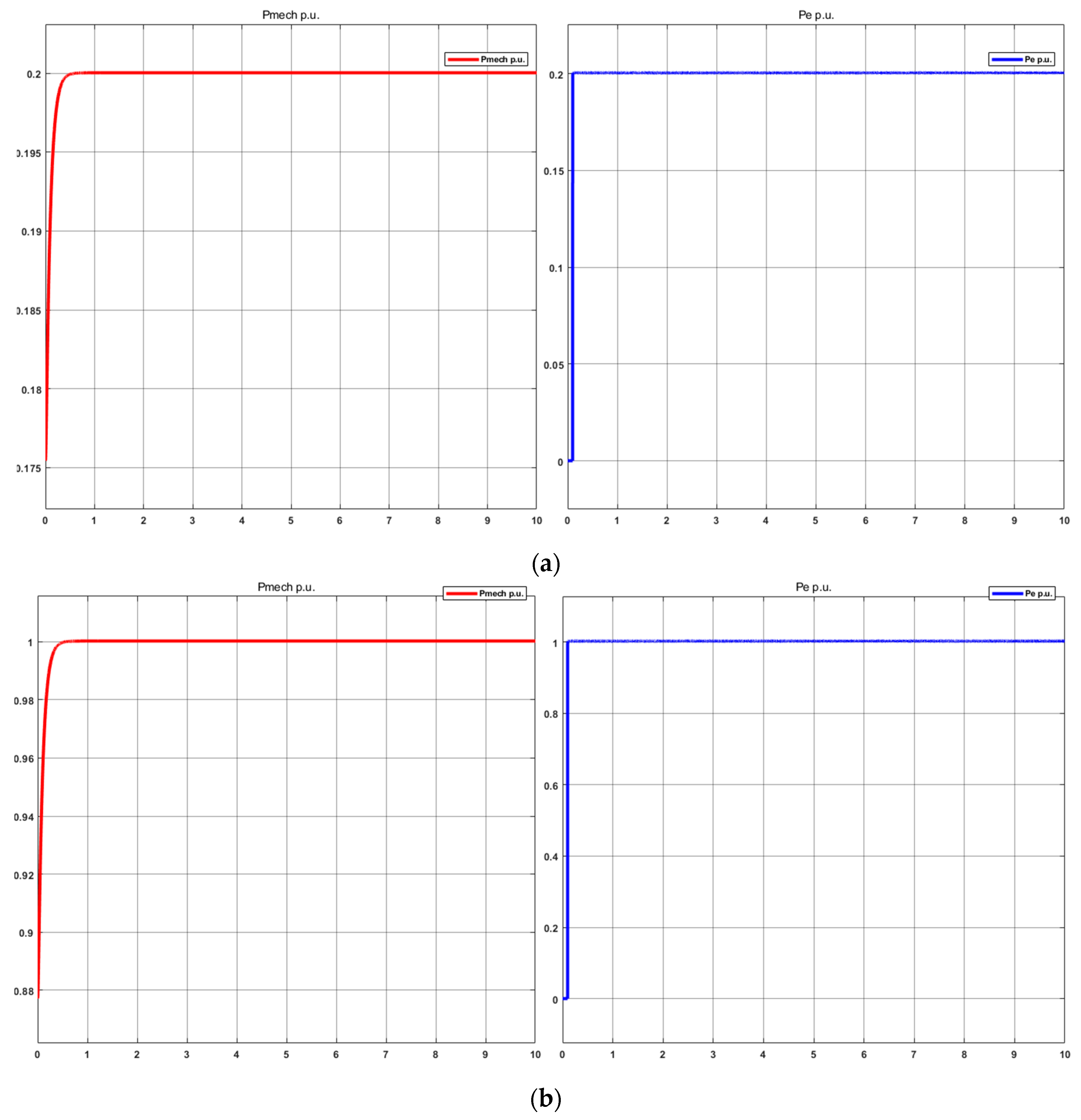
- Checking of nominal values:
- 2.
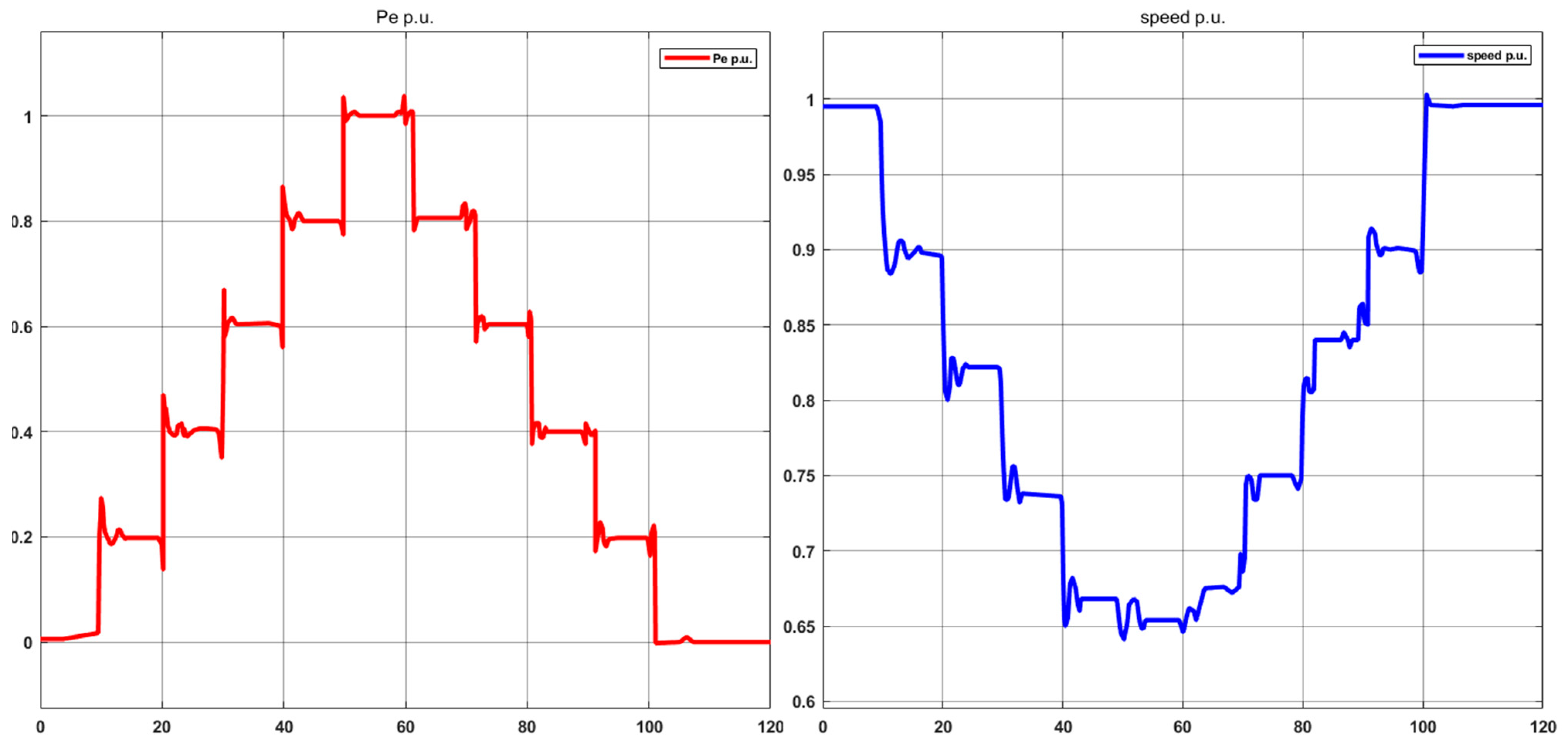
- Dynamic load requirement variation:
- The average settling times for state transitions resulting from variations in the load requirement of a 1 kW are: 3.76 s for up states and 2.92 s for the down states, with the times being slightly lower for down states;
- Although the dynamic behavior of the flows referenced in Table 16 shows a certain regularity and proportionality oriented towards a linear behavior, these behaviors are not reflected in the establishment times; because a more stable system is not available for these variations, work continues on the regularization of the control strategies used;
- There is a logical behavior in the fuel flow consumption, which is reflected in the variation in the air flow and mass flow, as more fuel flow is required when there is a higher load requirement, and with the opposite behavior being observed when there is a lower load requirement, requiring less fuel flow, air flow, and mass flow of steam;
- The rotor speed variation in the simple synchronous machine presents more irregularities due to the behavior of the non-linear parameters of the mathematical model, which are translated in the simulation into more abrupt changes due to the transitions in the load requirement states. The control strategies must be able to linearize the damping factor and the deviation from the nominal operating speed.
- 3.
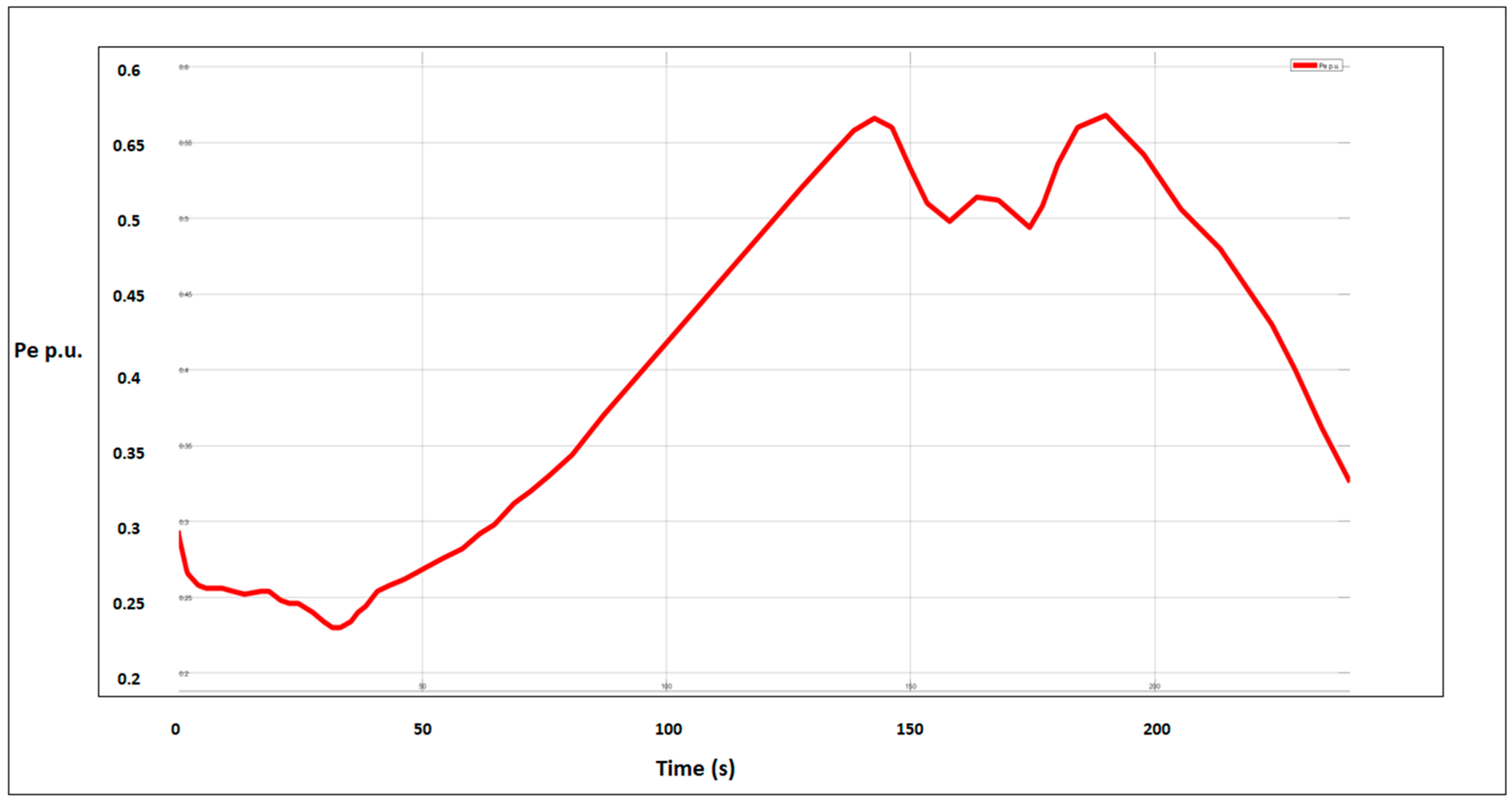
- Contrast variation in consumption profile and plant model
- There is a drop in load from hours 1 to 4, which is observed in the simulation between 0 and 40 s;
- From hour 5 to hour 12 in the Excel graph and from 50 to 150 s in the simulation, there is a higher demand for load;
- From 13 to 18 h, there is a decrease in the demand for load, which is also observed in the simulation between 130 and 180 s;
- There is an increase in consumption again between 18 and 20 h, which is observed in the simulation between 180 and 190 s;
- Finally, from hour 21 to 24 and from 190 to 240 s in the simulation, there is a drop in the demand for load.
- A classification of the studies consulted is proposed and generated, whether they are thermodynamic, techno-economic, based on simulation with specialized software, and mathematical, which is the main object of this work. The proposal is made in this way because, in all of the reference consultations, no differentiation is made, which generates confusion and mixture between models, which does not indicate that the models discard each other;
- Mathematical verification of each equation implemented in each subsystem of the plant, initially in Excel and later in Matlab/Simulink in the simulations which were carried out.
- Detailed presentation of all mathematical models, with equations, parameters, and values obtained if they are calculations, constants, and units. In most references which were consulted, especially articles, no further details of the models can be found;
- Results were obtained for a proposal for small-scale generation, facilitating sizing, where the gas turbine model is the most suitable plant option for these applications, as it provides fewer complex calculations, dynamics, and control. The mathematical model was mostly linear with the application of algebraic equations, and the most dynamic sequences are found in the fuel and control systems;
- The load requirements determine the fuel flow requirements, which affects the air and steam mass flows; consequently, it also affects the mechanical power, electrical power, rotor speed, and transition times both up and down, affecting the stability and reliability of the system. To improve this behavior, the responses of the control strategies must be further adjusted and sensitized;
- For an integration application in a hybrid microgrid where more energy resources are involved, control strategies more akin to a management system must be considered and developed.
4. Conclusions
Author Contributions
Funding
Institutional Review Board Statement
Informed Consent Statement
Data Availability Statement
Conflicts of Interest
References
- Herbert, G.M.J.; Krishnan, A.U. Quantifying Environmental Performance of Biomass Energy. Renew. Sustain. Energy Rev. 2016, 59, 292–308. [Google Scholar] [CrossRef]
- Yilmaz, F.; Ozturk, M.; Selbas, R. Design and Thermodynamic Assessment of a Biomass Gasification Plant Integrated with Brayton Cycle and Solid Oxide Steam Electrolyzer for Compressed Hydrogen Production. Hydrog. Energy 2020, 45, 34620–34636. [Google Scholar] [CrossRef]
- Trninić, M.; Stojiljković, D.; Manić, N.; Skreiberg, Ø.; Wang, L.; Jovović, A. A Mathematical Model of Biomass Downdraft Gasification with an Integrated Pyrolysis Model. Fuel 2020, 265, 116867. [Google Scholar] [CrossRef]
- Ordys, A.W.; Pike, A.W.; Johnson, M.A.; Katebi, R.M.; Grimble, M.J. Process Models. In Modelling and Simulation of Power Generation Plants; Springer: Berlin/Heidelberg, Germany, 2000; Chapter 4; pp. 144–208. [Google Scholar]
- Saravanamuttoo, H.I.H.; Cohen, H.; Rogers, G.F.C. Introduction. In Gas Turbine Theory, 5th ed.; Pearson: London, UK, 2013; Chapter 1; pp. 38–44. [Google Scholar]
- Jurado, M.F.; Cano, O.A. Capítulo 5 Microturbina de Gas. In Generación Eléctrica Distribuida Con Microturbina de Gas; Koobeht International, European Union: Jaén, Spain, 2005; pp. 187–205. [Google Scholar]
- Ortega, V.M. Modelado y Simulación Dinámica de Esquemas de Cogeneración. Doctorado Thesis, Universidad Autónoma de Nuevo León, Monterrey, Mexico, 2001. [Google Scholar]
- Hussain, A.; Seifi, H. Dynamic Modeling of a Single Shaft Gas Turbine. IFAC Control. Power Plants Power Syst. 1992, 25, 43–48. [Google Scholar] [CrossRef]
- Serrato Monroy, C.C.; Lesmes Cepeda, V. Metodología Para El Cálculo de Energía Extraída a Partir de La Biomasa En El Departamento de Cundinamarca, Ingeniería; Universidad Distrital: Bogotá, Colombia, 2016; p. 79. [Google Scholar]
- Ramirez Balaguera, L.F.; Barrera Ojeda, D.F. Potencial Energético de La Biomasa Residual Pecuaria Del Departamento de Cundinamarca–Colombia, Ingeniería; Universidad Distrital: Bogotá, Colombia, 2017; p. 147. [Google Scholar]
- Pozzobon, V.; Salvador, S.; Bézian, J. Biomass Gasification under High Solar Heat Flux_Advanced Modelling_Elsevier Enhanced Reader. Fuel 2018, 214, 300–313. [Google Scholar] [CrossRef]
- Toklu, E. Biomass Energy Potential and Utilization in Turkey. Renew. Energy 2017, 107, 235–244. [Google Scholar] [CrossRef]
- Nunes, L.J.R.; Matias, J.C.O.; Catalão, J.P.S. Biomass in the Generation of Electricity in Portugal: A Review. In Renewable and Sustainable Energy Reviews; Elsevier Ltd.: Amsterdam, The Netherlands, 2017; pp. 373–378. [Google Scholar] [CrossRef]
- Caliano, M.; Bianco, N.; Graditi, G.; Mongibello, L. Analysis of a Biomass-Fired CCHP System Considering Different Design Configurations. Energy Procedia 2017, 105, 1683–1691. [Google Scholar] [CrossRef]
- Ashok, S.; Balamurugan, P. Biomass Gasifier Based Hybrid Energy System for Rural Areas. In Proceedings of the 2007 IEEE Canada Electrical Power Conference, EPC, Montreal, QC, Canada, 25–26 October 2007; pp. 371–375. [Google Scholar] [CrossRef]
- Gómez, B.S. Diseño e Implementación de Un Sistema de Aprovechamiento de Residuos Orgánicos y Generación de Energía Renovable, Ingeniería; Universidad ECCI: Bogotá, Colombia, 2017; p. 89. [Google Scholar]
- CIGEPI. Eficiencia de Calderas Para El Uso de Biomasa; Superintendencia de Industria y Comercio: Antioquia, Colombia, 2017; p. 68.
- UPME; IDEAM; COLCIENCIAS; UIS. Anexo B Muestreo y Caracterización de La Biomasa Residual En Colombia. In Atlas del Potencial Energético de la Biomasa Residual en Colombia; República de Colombia ministerio de Minas y Energía: Bogotá, Colombia, 2013; pp. 131–142. [Google Scholar]
- Jiang, R.; Tong Wang, T.; Shao, J.; Guo, S.; Zhu, W.; Jun Yu, Y.; Lin Chen, S.; Hatano, R. Modeling the Biomass of Energy Crops: Descriptions, Strengths and Prospective. J. Integr. Agric. 2017, 16, 1197–1210. [Google Scholar] [CrossRef]
- UPME; Aene. Potencialidades de Los Cultivos Energéticos y Residuos Agrícolas en Colombia. In Resumen Ejecutivo; República de Colombia ministerio de Minas y Energía: Bogotá, Colombia, 2003; D.#ANC-631-03,REVISON 1; pp. 98–129. [Google Scholar]
- Cao, Y.; Mihardjo, L.W.W.; Dahari, M.; Tlili, I. Waste Heat from a Biomass Fueled Gas Turbine for Power Generation via an ORC or Compressor Inlet Cooling via an Absorption Refrigeration Cycle: A Thermoeconomic Comparison. Appl. Therm. Eng. 2021, 182, 116117. [Google Scholar] [CrossRef]
- Cirillo, D.; Di Palma, M.; La Villetta, M.; Macaluso, A.; Mauro, A.; Vanoli, L. A Novel Biomass Gasification Micro-Cogeneration Plant: Experimental and Numerical Analysis. Energy Convers. Manag. 2021, 243, 114349. [Google Scholar] [CrossRef]
- Elfasakhany Ashraf. Investigation of Biomass Powder as a Direct Solid Biofuel in Combustion. Ain Shams Eng. J. 2021, 12, 2991–2998. [Google Scholar] [CrossRef]
- Hussain, C.M.I.; Norton, B.; Duffy, A. Comparison of Hybridizing Options for Solar Heat, Biomass and Heat Storage for Electricity Generation in Spain. Energy Convers. Manag. 2020, 222, 113231. [Google Scholar] [CrossRef]
- Akrami, E.; Ameri, M.; Rocco, M.V. Developing an Innovative Biomass-Based Power Plant for Low-Carbon Power Production: Exergy and Exergoeconomic Analyses. Therm. Sci. Eng. Prog. 2020, 19, 100662. [Google Scholar] [CrossRef]
- Roy, D.; Samanta, S.; Ghosh, S. Performance Assessment of a Biomass Fuelled Advanced Hybrid Power Generation System. Renew. Energy 2020, 162, 639–661. [Google Scholar] [CrossRef]
- Bisht, A.S.; Thakur, N.S. Small Scale Biomass Gasification Plants for Electricity Generation in India: Resources, Installation, Technical Aspects, Sustainability Criteria & Policy. Renew. Energy Focus 2019, 28, 112–126. [Google Scholar] [CrossRef]
- Sandoval, L.P.; Díaz, C.A. Sustainability Aspects of Biomass Gasification Systems for Small Power Generation. Renew. Sustain. Energy Rev. 2020, 134, 110180. [Google Scholar]
- Herrera, I.; Rodríguez-Serrano, I.; Lechón, Y.; Oliveira, A.; Krüger, D.; Bouden, C. Sustainability Assessment of a Hybrid CSP/Biomass. Results of a Prototype Plant in Tunisia. Sustain. Energy Technol. Assess. 2020, 42, 100862. [Google Scholar] [CrossRef]
- Rey, J.R.C.; Pio, D.T.; Tarelho, L.A.C. Biomass Direct Gasification for Electricity Generation and Natural Gas Replacement in the Lime Kilns of the Pulp and Paper Industry: A Techno-Economic Analysis. Energy 2021, 237, 321–330. [Google Scholar] [CrossRef]
- Krzysztof, S.; Maciej, Z.; Wojciech, G.; Rafal, F. The Operation of a Micro-Scale Cogeneration System Prototype–A comprehensive experimental and numerical analysis. Fuel 2021, 295, 1–18. [Google Scholar]
- Safarian, S.; Ebrahimi Saryazdi, S.M.; Unnthorsson, R.; Richter, C. Artificial Neural Network Integrated with Thermodynamic Equilibrium Modeling of Downdraft Biomass Gasification-Power Production Plant. Energy 2020, 213, 491–512. [Google Scholar] [CrossRef]
- Chiñas-Palacios, C.; Vargas-Salgado, C.; Aguila-Leon, J.; Hurtado-Pérez, E. A Cascade Hybrid PSO Feed-Forward Neural Network Model of a Biomass Gasification Plant for Covering the Energy Demand in an AC Microgrid. Energy Convers. Manag. 2021, 232, 113896. [Google Scholar] [CrossRef]
- Cerinski, D.; Baleta, J.; Mikulčić, H.; Mikulandrić, R.; Wang, J. Dynamic Modelling of the Biomass Gasification Process in a Fixed Bed Reactor by Using the Artificial Neural Network. Clean Eng. Technol. 2020, 1, 100029. [Google Scholar] [CrossRef]
- Ribó-Pérez, D.; Herraiz-Cañete, Á.; Alfonso-Solar, D.; Vargas-Salgado, C.; Gómez-Navarro, T. Modelling Biomass Gasifiers in Hybrid Renewable Energy Microgrids; a Complete Procedure for Enabling Gasifiers Simulation in HOMER. Renew. Energy 2021, 174, 501–512. [Google Scholar] [CrossRef]
- Ahluwalia, K.S.; Domenichini, R. Dynamic Modelling of a Combined Cycle Plant. ASME 1989, 79160, V004T09A009. [Google Scholar]
- Hung, W.W. Dynamic Simulation of Gas-Turbine Generating Unit. IEE Proc. 1991, 138, 342–350. [Google Scholar] [CrossRef]
- Rowen, W.I. Simplified Mathematical Representations of Heavy Duty Gas Turbines. ASME 1983, 105, 865–869. [Google Scholar] [CrossRef]
- Barker, W.; Cronin, M. Speedtronic Mark IV Control System, Alsthom Gas Turbine Reference Library. 2000, Volume 4193A. Available online: https://vdocuments.mx/ger-4193a-speedtronic-mark-vi-turbine-control-system-2021-4-6-speedtronica.html?page=1 (accessed on 20 April 2023).
- Yacobucci, R.B. A Control System Retrofit for a GE Frame 5 Turbine Generator Unit. IEEE Trans. Energy Convers. 1991, 6, 225–230. [Google Scholar] [CrossRef]
- Jurado, F.; Ortega, M.; Cano, A. Neuro-Fuzzy Controller for Gas Turbine in Biomass-Based Electric Power Plant. Electr. Power Syst. Res. 2002, 60, 123–135. [Google Scholar] [CrossRef]
- Zhu, Z.; Wang, X.; Xie, D.; Gu, C. Control Strategy for MGT Generation System. Energies 2019, 12, 3101. [Google Scholar] [CrossRef]
- Jonathan, A.E.; Olubiwe, M.; Okozi, S.O.; Agubor, C.K. Exhaust Temperature Control of Heavy Duty Gas Turbine Due to Incremental Load Demand. Int. J. Eng. Res. Technol. 2018, 7, 420–426. [Google Scholar] [CrossRef]
- Shankar, G.; Mukherjee, V. Load-Following Performance Analysis of a Microturbine for Islanded and Grid Connected Operation. Int. J. Electr. Power Energy Syst. 2014, 55, 704–713. [Google Scholar] [CrossRef]
- El-Sharif, I.A.; El-Fandi, M.M. Micro Gas Turbine Simulation and Control. In Proceedings of the Conference for Engineering Sciencies and Technology (CEST), Castelverde, Libya, 25–27 September 2018; pp. 1–10. [Google Scholar]
- Shakur, S.A.; Jain, S.K. Micro-Turbine Generation Using Simulink. Int. J. Electr. Eng. 2012, 5, 95–110. [Google Scholar]
- Guda, S.R.; Wang, C.; Nehrir, M.H. Modeling of Microturbine Power Generation. Electr. Power Compon. Syst. 2006, 34, 1027–1041. [Google Scholar] [CrossRef]
- Singh, N.K.; Tiwari, P.; Srivastava, J. Simulation Of Microturbine Generation System For Unbalance Grid Power. Int. J. Eng. Res. Technol. 2013, 2, 967–974. [Google Scholar]
- Abdollahi, S.E.; Vahedi, A. Dynamic Modelling of Micro-Turbine Generation Systems Using Matlab/Simulink. Renew. Energy Power Qual. J. 2005, 1, 146–152. [Google Scholar] [CrossRef]
- Herrador, C.M. Modelado En Matlab-Simulink de Generadores Eléctricos Conectados a La Red; Universidad de Sevilla: Sevilla, Spain, 2016. [Google Scholar]
- Chiguano, B.A. Estimación de Parámetros Eléctricos de La Máquina Sincrónica Utilizando Matlab-Simulink. Bachelor’s Thesis, Escuela Politecnica Nacional, Quito, Ecuador, 2018. [Google Scholar]
- Sistemas de Generación. Generadores Síncronos y Asíncronos. Available online: https://biblus.us.es/bibing/proyectos/abreproy/4991/fichero/4+Sistemas+de+generaci%C3%B3n.pdf (accessed on 4 April 2023).
- Sistema Interconectado Nacional. Indicadores de Pronósticos Oficiales de Demanda. Available online: https://www.xm.com.co/consumo/informes-demanda/indicadores-de-pronosticos-oficiales-de-demanda (accessed on 2 April 2023).
- Consejo Nacional de Operaciones-CNO. Acuerdo 1303 Por el Cual se Actualizan los Procedimientos Para la Gestión Integral de la Demanda. Available online: https://www.cno.org.co/content/acuerdo-1303-por-el-cual-se-actualizan-los-procedimientos-para-la-gestion-integral-de-la (accessed on 2 April 2023).
- Enel-Codensa. Innovación y Sostenibilidad. Available online: https://www.enel.com.co/es/medio-ambiente-desarrollo-sostenible.html (accessed on 2 April 2023).


| Source | Advantages | Disadvantages |
|---|---|---|
| [11] | Renewable energy source | May require processing |
| [12] | Reduction of greenhouse gas emissions | Combustion generates ash and tar |
| [13] | Waste reduction | Limited availability |
| [14] | Contribution to rural development | Requires space and resources |
| [15] | Local production | Can compete with food production |
| Type of Crop | Type of Waste | LCV (kcal/kg) | Energy Potential (TJ/Year) | Energy Potential (GWh/Year) |
|---|---|---|---|---|
| Oil Palm | Fart | 3.988 | 239.29 | 66.471 |
| Fibre | 4.274 | 618.24 | 171.733 | |
| Palm rachis | 4.021 | 601.11 | 166.974 | |
| Panelera Cane | Bagasse | 4.456 | 9524.84 | 2645.791 |
| Leaves—Bud | 4.007 | 2866.22 | 796.173 | |
| Coffee | Pulp | 4.259 | 217.76 | 60.489 |
| Cisco | 4.430 | 100.73 | 27.981 | |
| Stems | 4.384 | 1165.21 | 323.67 | |
| Corn | Stubble | 3.429 | 318.01 | 88.336 |
| Tusa | 3.390 | 97.27 | 27.019 | |
| Doormat | 3.815 | 110.88 | 30.8 | |
| Rice | Tamo | 3.113 | 143.98 | 39.995 |
| Husk | 3.603 | 49.63 | 13.787 | |
| Banana | Banana rachis | 1.809 | 12.05 | 3.347 |
| Banana stem | 2.032 | 79.15 | 21.986 | |
| Rejected banana | 2.488 | 7.4 | 2.056 | |
| Plantain | Plantain rachis | 1.808 | 10.03 | 2.786 |
| Plantain stem | 2.032 | 65.88 | 18.3 | |
| Rejected plantain | 2.480 | 6.16 | 1.711 |
| Equation | Parameter | Description | Value | Unit |
|---|---|---|---|---|
| PE | Energy Potential | [TJ/year] | ||
| Mass of dry residue | [t/year] | |||
| E | Energy of the residue per unit mass | [TJ/t] | ||
| A | Cultivated area | [ha/year] | ||
| Crop yield | [t main product/ha planted] | |||
| Mass of residue generated from the cultivation | [t of waste/t of main product] | |||
| Dry residue fraction | [t dry residue/t wet residue] | |||
| “k” “i” | Biomass classification Types of waste biomass | [t/year] | ||
| Unit conversion constant | 1 × 10⁻⁶ | |||
| The overall energy potential of agricultural waste biomass | ||||
| PCI | Lower Caloric Value of the residue | [TJ/t] |
| Equation | Parameter | Description | Value | Unit |
|---|---|---|---|---|
| Biomass | Biomass quantity | |||
| Power | Power required | [kW] | ||
| PCI | Lower Calorific Value | |||
| PCI | Lower Calorific Value | 4.384 | ||
| cal | 1 calorie | 4.1855 | kJ | |
| cal | Product | 18.349232 | ||
| Power required | ||||
| Biomasa | Quantity of biomass required to produce 1 kW | 0.215 |
| Source | Description | Process | Contribution |
|---|---|---|---|
| [2] | The complete evaluation of the thermodynamic performance of an integrated biomass-supported combined plant is investigated. For thermodynamic investigation, the mass, energy, entropy, and exergy balance relationships of the modelled plant and sub-plants are applied. | Biomass gasification | It performs a comprehensive thermodynamic calculation of the combined cycle supported by biomass gasification to produce electric heat, fresh water, and hydrogen. |
| [21] | Gasification modelling procedures fall into two main categories: equilibrium and kinetic models. | Biomass gasification | Develop a code using MATLAB software to apply the GA procedure for the purpose of system optimization from thermodynamic and economic perspectives. |
| [22] | It presents the simulation of a real mCHP plant, based on a biomass gasifier coupled to an internal combustion engine (ICE), in the Aspen Plus environment to predict the system behavior. | Biomass gasification | The model reproduces the operation of the syngas cleaning unit, the ICE, and the thermal recovery system. In particular, the thermal recovery system has been reproduced by implementing the detailed geometrical characteristics of the actual heat exchangers of the mCHP with Aspen EDR environment. |
| [23] | They propose computational fluid dynamics (CFD) simulation validated against experiments. | Biomass gasification | The results showed that all models can represent biomass combustion in a reasonable way. Biomass gasification is completed at a temperature of 1050 °K. |
| [3] | They develop and implement a zero-dimensional model for downdraft biomass gasification in fixed-bed or slow-bed gasifiers. | Biomass gasification | The proposed model considers the main gasification sub-processes (drying, pyrolysis, gasification) and their products. The model successfully predicts the conversion behaviors of different types of biomasses during a gasification process in terms of yield and product composition. |
| Source | Description | Process | Contribution |
|---|---|---|---|
| [24] | The study shows that various techno-economic parameters have significant effects on the reduction of the normalized cost of electricity—LCOE in different power plant configurations. | CSP-biomass-TES hybrid power plant. | In the paper, they model and simulate three power plant configurations to calculate the cost of electricity for each. |
| [25] | They propose a novel concept of BECCS (Bioenergy with carbon capture and storage) for energy production. | Downdraft gasifier | The innovative energy system presented is defined based on the integration of a downdraft gasifier, an external combustion gas turbine, an MCFC section, an organic Rankine cycle and a cryogenic CO2 capture. The proposed system is modelled and analyzed on the basis of exergy and exergy-economic analysis. |
| [26] | They evaluate the performance of an advanced biomass-fueled hybrid power generation system and model a modern biomass-based electrochemical power generation system. | Biomass gasifier, SOFC, Direct Combustion GT and ORC. | They present a detailed parametric study of the system to exhibit thermo-economic and environmental behaviors. |
| [27] | They present the latest statistical data on energy generation from bioenergy resources using available sources. | Biomass gasification | They include descriptions of gasification conversion routes, with their sustainability conditions, as well as the government policies necessary for their implementation in the Indian context. |
| [28] | A review of the sustainability aspects of biomass gasification and the use of biomass synthesis gas for small-scale power generation is presented, taking the UN Sustainable Development Goals (ODS) as a frame of reference. | Synthesis gas from biomass | The sustainability framework provided by the ODS, together with the concepts of energy transition and the energy trilemma, give bioenergy great importance in what should be its participation in an energy matrix geared towards distributed energy systems. |
| [29] | It assesses the feasibility of new renewable energy systems, and analyses the sustainability impact of these technologies along the entire supply chain in the environmental, social, and economic pillars. | Systems of Renewable energy | They consider not only the cost of energy but also the environmental and socio-economic impacts involved throughout the life cycle of the technology. |
| [30] | They present an analysis to achieve the EU’s goals of a climate-neutral economy by 2050, highlighting that an adjustment of the current economy to one based on renewable raw materials (bioeconomic) must take place. | Bioeconomic | They stress that renewable solutions should be introduced into our existing production chain and should be conceived not as immediate solutions, but as long-term solutions, to be used as early as possible and improved over time. |
| [31] | They present an analysis of micro-scale biomass-fueled applications, with wood, straw, energy crop plants, and agricultural products being the most used fuels. | Applications Microscale | They study various types of boilers for each type of biomass, resulting from different fuel properties and investors’ expectations (e.g., in relation to price and operational parameters such as the convenience of use). |
| Source | Description | Process | Contribution |
|---|---|---|---|
| [32] | They point out that there are very few published studies on the modelling of biomass gasification based on the ANN method and even fewer in the field of fixed-bed downdraft gasifiers. | Biomass gasification based on the ANN method | They develop an integrated ANN model with a thermodynamic equilibrium approach for the downstream biomass gasification integrated power generation unit, which aims to predict the net power output of systems derived from various types of biomass feedstocks under atmospheric pressure and various operating conditions. |
| [33] | It presents an Artificial Neural Network (ANN) based model hybridized with a Particle Swarm Optimization (PSO) algorithm for a Biomass Gasification Plant (BGP) to estimate the amount of biomass needed to produce the syngas required to satisfy the energy demand. | Biomass gasification plant | The proposed model is compared with two traditional ANN models: Backward Feedback Propagation (FF-BP) and Forward Cascade Propagation (CF-P). ANNs are trained in MATLAB software using a real historical data set from a BGP located in the Distributed Energy Resources Laboratory of the Universitat Politècnica de València in Spain. |
| [34] | They researched about the possibility of using NARX ANN in a fixed-bed downdraft gasifier to predict syngas composition for lower data logging frequency. | Biomass downdraft fixed-bed downdraft gasifier | They obtain results from an open-loop network consisting of input and output layers connected with a hidden layer of 5 neurons. The application of the network allows online prediction and control of the gasification process. |
| [35] | They present two case studies that combining PV, biomass gasifier and batteries; one in Honduras and the other in Zambia. | Biomass gasification | The simulation resulting from the research allowed to review the performance of a gasifier in two HRES case studies that combine PV, biomass gasifier and batteries; one in Honduras and the other in Zambia. |
| Source | Description | Process | Contribution |
|---|---|---|---|
| [4] | The book presents comprehensive information on CC combined cycle and CHP combined heat and power cycle systems. | Biomass gasification | It presents in detail the mathematical, control, and simulation models of gas turbine, steam turbine, and combined gas turbine-based power plants. From the book the following references are highlighted [8,28,36,37,38,39,40], being the basis for the development and application of gas turbines. |
| [6] | The book presents comprehensive information on distributed generation using gas microturbines, apart from mathematical models, it highlights control models and microgrid applications. | Distributed electricity generation with gas microturbine | Control models and micro-grid oriented applications are highlighted. |
| [7] | In the Thesis, it is applied the dynamic models described in the book [27] by generating simulations of gas, steam, and combined cycle turbine plants, which validate the models for his own application. | Modeling and dynamic simulation of cogeneration schemes | It presents simulations of gas, steam, and combined cycle turbine plants, which validate the models for their own application. |
| [41] | It presents an application of mathematical models oriented to simulation and control based on neuro-fuzzy controllers, controlling several scenarios of variation of power, torque, active, and reactive load. | Neuro-fuzzy Control | Neuro-fuzzy controller applied to various scenarios of variation of power, torque, active, and reactive load. |
| [42,43,44,45,46,47,48,49] | They are based on the same mathematical and control models | Gas turbine | There is no great detail of the mathematical models, calculations, or parameters of each subsystem, each study focuses its development on specific applications. |
| Equation | Parameter | Description | Value | Unit | Procedure |
|---|---|---|---|---|---|
| Wf | Fuel mass flow. | 2.889 × 10⁻⁴ | kg/s | Calculation | |
| kff | System Gain. | 1 | No Unit | Parameter | |
| τf | System time constant. | 0.01 | s | Parameter | |
| e1 | Valve positioner. | dynamic | No Unit | Calculation | |
| a, b, c | Valve parameters. | 10, 1, 0 | No Unit | Parameter | |
| e2 | Internal positioning signal. | dynamic | No Unit | Calculation | |
| MF | Minimum fuel signal. | 0.8 | p.u. | Calculation | |
| kf | Feedback coefficient. | 1 | No Unit | Parameter | |
| Fd | Fuel demand signal. | 1 | p.u. | Calculation | |
| Turbine speed. | 188.45 | rad/s | Calculation | ||
| τ | System time delay. | 0.01 | s | Parameter |
| Equation | Parameter | Description | Value | Unit | Procedure |
|---|---|---|---|---|---|
| wa | Air mass flow inside the compressor. | 5.767 × 10⁻¹ | kg/s | Calculation | |
| A0 | Compressor outlet area. | 1.2 × 10⁻² | m2 | Parameter | |
| η∞c | Polytropic compressor efficiency. | 0.9 | No Unit | Parameter | |
| ρi | Inlet air density. | 1.21 | kg/m3 | Parameter | |
| pcin | Inlet air pressure. | 15.62 | Pa | Parameter | |
| ma | Polytropic index. | 1.417 | No Unit | Calculation | |
| rc | Pressure ratio (pout/pin). | 10 | No Unit | Calculation | |
| γa | (cpa/cva) Specific heat ratio for air (constant). | 1.411 | No Unit | Calculation | |
| cpa | Specific heat of air at constant pressure. | 1.012 | J/(kg °K) | Parameter | |
| cva | Specific heat of air at constant volume. | 0.717 | J/(kg °K) | Parameter | |
| rc | Pressure ratio (pout/pin). | 10 | No Unit | Calculation | |
| pcout | Outlet air pressure | 156 | Pa | Calculation | |
| Tcout | Outlet air temperature | 547 | °K | Calculation | |
| Tcin | Inlet air temperature. | 288 | °K | Parameter | |
| Pc | Compressor power consumption | 1820 | W | Calculation | |
| ∆hI | isoentropic enthalpy change. Corresponding to the compression of Pcin with respect to Pcout | 2.698 × 10⁵ | J/kg | Calculation | |
| ηc | Total compressor efficiency. | 0.863 | No Unit | Calculation | |
| ηtrans | Transmission efficiency from turbine to compressor. | 0.99 | No Unit | Parameter | |
| ηc | Total compressor efficiency. | 0.863 | No Unit | Calculation | |
| cpair | Specific heat of air at constant pressure. | 1005 | J/(kg °K) | Parameter | |
| Rair | Ideal gas constant for air. | 287 | J/(kg °K) | Parameter |
| Equation | Parameter | Description | Value | Unit | Procedure |
|---|---|---|---|---|---|
| wG | Outlet gas mass flow. | 5.77 × 10⁻¹ | kg/s | Calculation | |
| wis | Steam mass flow injection. | 2.9 × 10⁻⁵ | kg/s | Calculation | |
| wf | Fuel mass flow to the turbine. | 2.88 × 10⁻⁴ | kg/s | Calculation | |
| Equation for the energy of combustion at temperature 25 °C, is cleared for TTin. | |||||
| cpg | Specific heat of flue gases | 1144 | J/(kg °K) | Parameter | |
| cps | Specific heat of steam. | 2005 | J/(kg °K) | Parameter | |
| cpa | Specific heat of air. | 1005 | J/(kg °K) | Parameter | |
| TTin | Turbine inlet gas temperature. | 1420 | °K | Calculation | |
| ∆h25 | Specific enthalpy of reaction at the reference temperature, (25 °C). | (−4.0 × 10⁷) | J/(kg) | Parameter | |
| Tis | Steam temperature. | 601 | °K | Parameter | |
| PTin | Loss of combustion chamber pressure. | 159 | Pa | Calculation | |
| ∆p | Loss of pressure in the combustion chamber. | 2.698 | Pa | Calculation | |
| k1, k2 | Pressure loss coefficients | 1 | No Unit | Parameter | |
| R | Universal gas constant for flue gases | 287 | J/(kg °K) | Constante | |
| Am | Cross-sectional area of the combustion chamber. | 1 | m2 | Parameter | |
| Tref | Reference combustion temperature. | 1000 | °K | Parameter | |
| href | Reference flue gas enthalpy. | 1.2 × 10⁶ | J/kg | Parameter | |
| hTin | Turbine inlet gas enthalpy. | 1.685 × 10⁶ | J/kg | Calculation |
| Equation | Parameter | Description | Value | Unit | Procedure |
|---|---|---|---|---|---|
| Ttout | Gas temperature at the turbine outlet. | 763 | °K | Calculation | |
| rT | pTout/pTin Turbine pressure ratio. | 6.29 × 10⁻² | No Unit | Calculation | |
| pTout | Turbine outlet air pressure. | 9.4 | Pa | Calculation | |
| η∞T | Polytropic turbine efficiency | 0.9 | No Unit | Parameter | |
| γcg | cpg/cvg, Specific heat ratio for flue gases. | 1.33 | No Unit | Calculation | |
| wG | Turbine gas mass flow | 5.77 × 10⁻¹ | kg/s | Calculation | |
| ATo | Turbine outlet area | 0.14 | m2 | Parameter | |
| η∞T | Polytropic turbine efficiency | 0.9 | No Unit | Parameter | |
| ρTin | Inlet gas density | 3.778 × 10⁻⁴ | kg/m3 | Calculation | |
| pTin | Turbine inlet air pressure. | 159 | Pa | Calculation | |
| mcg | Polytropic flue gas index. | 1.384 | No Unit | Calculation | |
| ρTin | Inlet gas density | 3.778 × 10⁻⁴ | kg/m3 | Calculation | |
| mcg | Polytropic flue gas index. | 1.384 | No Unit | Calculation | |
| rT | pTout/pTin Turbine pressure ratio. | 6.29 × 10⁻² | No Unit | Calculation | |
| ηT | Overall turbine efficiency. | 0.931 | No Unit | Calculation | |
| ∆hI cpg Rcg | Isentropic enthalpy change. Specific heat of flue gas. Ideal gas constant for gas. | 1.27 × 10⁴ 1144 287 | J/(kg °K) J/(kg °K) J/(kg °K) | Calculation Parameter Parameter | |
| hTout | Enthalpy of the turbine exhaust gases. | 1.697 × 10⁶ | J/kg | Calculation | |
| PT | Mechanical power delivered by the turbine. | 6820 | W | Calculation | |
| Pc | Power required by the compressor. | 1820 | W | Calculation | |
| Pmech | Net mechanical power available in the turbine. | 5000 | W | Calculation |
| Advantages | Disadvantages |
|---|---|
| Synchronous Generator | |
| Greater efficiency | Greater complexity |
| Increased stability | Requires an excitation source |
| Lower long-term cost | Higher initial cost |
| Reactive power | Increased maintenance |
| Good power quality | Accurate grid synchronization |
| Low noise | Increased inertia |
| Greater responsiveness to load variations | Increased sensitivity to network disturbances |
| Accuracy in frequency control | |
| Asynchronous generator | |
| Simplicity | Lower efficiency |
| Does not require an excitation source | Lower power quality |
| Lower initial cost | Slower response time |
| No regular maintenance required | No regular maintenance required |
| Increased capacity to withstand network disturbances | |
| Equation | Parameter | Description | Value | Unit | Procedure |
|---|---|---|---|---|---|
| Δω(t) | Deviation from nominal operating speed | dynamic | rad/s | Calculation | |
| H | Inertia constant | 3 | s | Parameter | |
| Tm | Mechanical torque | N/m | Parameter | ||
| Te | Electromagnetic torque | N/m | Parameter | ||
| kd | Damping factor | 64.3 | pu | Calculation | |
| ω(t) | Mechanical rotor speed | 188.45 | rad/s | Parameter | |
| ω0 | Nominal operating rotor speed | 188.45 | rad/s | Calculation |
| Control | Parameter | Description | Value | Units |
|---|---|---|---|---|
| Electrical Power: Pe | Pe_pu | Signal power generator | 1 | p.u. |
 | Pe_set_pu | Reference signal generator power | ||
| PI_Pe | Proportional—Integral | |||
| P | Proportional | |||
| I | Integral | |||
| Rotor Speed: ω | ω_pu | Rotor speed of operation | p.u. | |
 | ω_set_pu | Reference rotor speed of operation | p.u. | |
| PID_ ω | Proportional—Integral—Derivative | |||
| P | Proportional | |||
| I | Integral | |||
| D | Derivative | |||
| Temperature: TTout | T_Tout_pu | Turbine outlet temperature | ||
 | Función CR | Radiation field | ||
| T_Tout_set_pu | Outlet reference temperature Turbine | |||
| FunciónT | Termocouple | |||
| P_T_Tout | Proportional_T_Tout | |||
| P | Proportional | |||
| PI_w_air | Proportional—Integral airflow | |||
| P | Proportional | |||
| I | Integral | |||
| Gases NOx: gcNOx | gcNOx | Mass flow of NOx | ||
 | wis | Steam mass flow inyection. | 2.9 × 10⁻⁵ | kg/s |
| wf | Fuel mass flow to the turbine. | 2.88 × 10⁻⁴ | kg/s | |
| fGT2 | Experimental curve: NOx steam mass flow to fuel ratio | |||
| gcNOx_set | Reference mass flow of NOx | |||
| Delay | 0.001 | |||
| Dead Zone | −0.1–0.1 | |||
| PI_w_is | Proportional—Integral mass flow of steam | |||
| P | Proportional | 0.0002 | ||
| I | Integral | 0.001 |
| Load (W) | Upward Transition Time (s) | Downward Transition Time (s) | wf (kg/s) Fuel Flow | wa (kg/s) Airflow | wis (kg/s) Steam Mass Flow |
|---|---|---|---|---|---|
| 1000 | 3.5 | 1.4 | 5.77938 × 10⁻⁵ | 0.115351848 | 5.80188 × 10⁻⁶ |
| 2000 | 5.2 | 3.7 | 0.000115588 | 0.230703695 | 1.16038 × 10⁻⁵ |
| 3000 | 3 | 2.5 | 0.000173381 | 0.346055543 | 1.74056 × 10⁻⁵ |
| 4000 | 4 | 3.5 | 0.000231175 | 0.46140739 | 2.32075 × 10⁻⁵ |
| 5000 | 3.1 | 3.5 | 0.000288969 | 0.576759238 | 2.90094 × 10⁻⁵ |
| Hour Day | Load Variation in W Reference File Figure 9 (W) | Load Variation in p.u. of the Simulation in Figure 10 (p.u.) | wf (kg/s) Fuel Flow | wa (kg/s) Airflow | wis (kg/s) Steam Mass Flow |
|---|---|---|---|---|---|
| 1–4 | 1486 1360 | 0.3 0.26 | 0.0000858815868 0.000078599568 | 0.1714128455336 0.156878512736 | 0.00000862159368 0.0000078905568 |
| 5–12 | 1499 2201 | 0.3 0.55 | 0.000078599568 0.0001272041538 | 0.1729124195524 0.2538894165676 | 0.00000869701812 0.2538894165676 |
| 13–18 | 2194 2034 | 0.57 0.48 | 0.0001272041538 0.0001175525892 | 0.2530819536344 0.2346256580184 | 0.2530819536344 0.2346256580184 |
| 18–20 | 2034 2202 | 0.48 0.56 | 0.0001175525892 0.0001272619476 | 0.2346256580184 0.2540047684152 | 0.2346256580184 0.2540047684152 |
| 21–24 | 2127 1587 | 0.45 0.38 | 0.0001272619476 0.0000917187606 | 0.2453533798452 0.1830633821412 | 0.2453533798452 0.00000920758356 |
Disclaimer/Publisher’s Note: The statements, opinions and data contained in all publications are solely those of the individual author(s) and contributor(s) and not of MDPI and/or the editor(s). MDPI and/or the editor(s) disclaim responsibility for any injury to people or property resulting from any ideas, methods, instructions or products referred to in the content. |
© 2023 by the authors. Licensee MDPI, Basel, Switzerland. This article is an open access article distributed under the terms and conditions of the Creative Commons Attribution (CC BY) license (https://creativecommons.org/licenses/by/4.0/).
Share and Cite
Rico-Riveros, L.F.; Trujillo-Rodríguez, C.L.; Díaz-Aldana, N.L.; Rus-Casas, C. Modelling of Electric Power Generation Plant Based on Gas Turbines with Agricultural Biomass Fuel. Electronics 2023, 12, 1981. https://doi.org/10.3390/electronics12091981
Rico-Riveros LF, Trujillo-Rodríguez CL, Díaz-Aldana NL, Rus-Casas C. Modelling of Electric Power Generation Plant Based on Gas Turbines with Agricultural Biomass Fuel. Electronics. 2023; 12(9):1981. https://doi.org/10.3390/electronics12091981
Chicago/Turabian StyleRico-Riveros, Luis Fernando, César Leonardo Trujillo-Rodríguez, Nelson Leonardo Díaz-Aldana, and Catalina Rus-Casas. 2023. "Modelling of Electric Power Generation Plant Based on Gas Turbines with Agricultural Biomass Fuel" Electronics 12, no. 9: 1981. https://doi.org/10.3390/electronics12091981