Lightweight Deep Learning Model for Real-Time Colorectal Polyp Segmentation

Abstract

In colonoscopy, computer vision and artificial intelligence technology have enabled the automatic detection of the location of polyps and their visualization. These advancements have facilitated considerable research in the field. However, deep learning models used in the segmentation problem for capturing various patterns of polyps are becoming increasingly complex, which has rendered their operation in real time difficult. To identify and overcome this problem, a study was conducted on a model capable of precise polyp segmentation while increasing its processing speed. First, an efficient, high-performance, and lightweight model suitable for the segmentation of polyps was sought; the performance of existing segmentation models was compared and combined to obtain a learning model that exhibited good accuracy and speed. Next, hyperparameters were found for the MobileNetV3-encoder-based DeepLabV3+ model and, after tuning the hyperparameters, quantitative and qualitative results were compared, and the final model was selected. The experimental results showed that this model achieved high accuracy, with a Dice coefficient of 93.79%, while using a limited number of parameters and computational resources. Specifically, the model used 6.18 million parameters and 1.623 giga floating point operations for the CVC-ClinicDB dataset. This study revealed that increasing the amount of computation and parameters of the model did not guarantee unconditional performance. Furthermore, for the search and removal of polyps in cases in which morphological information is critical, an efficient model with low model complexity and high accuracy was proposed for real-time segmentation.

1. Introduction

Colorectal cancer is a malignant tumor that occurs in the mucous membranes of the colon or rectum. Malignant tumors not only grow indefinitely, but also involve transfer to surrounding tissues, causing the destruction of the body’s tissues, which can result in death if the normal function of the body is obstructed. Furthermore, if it is not removed through chemotherapy or surgery, cancer is rarely alleviated naturally and is more likely to continue to grow.

The symptoms of colorectal cancer include changes in bowel habits, rectal bleeding, abdominal tumors, abdominal pain, unprecedented weight loss, and anemia. Because these clinical symptoms may be caused by diseases other than colon cancer, additional tests such as colon angiography, blood tests, and colonoscopy should be conducted [1,2]. Records have revealed that of more than 1.9 million patients suffering from colorectal cancer, more than 930,000 deaths have been reported worldwide, and the risk of this disease is statistically proven [1]. The continuous increase in the mortality rate of colorectal cancer can be attributed to the failure to detect cancer at an early stage.

An effective method for the early detection of colorectal cancer is colonoscopy, which involves the visual diagnosis of diseases in the large intestine by inserting a charged-couple device camera or fiber optic camera into the intestine through the rectum. Colonoscopy enables visual checking of the rectum and large intestine and, because this process is noninvasive, colon diseases can be evaluated with low risk. Furthermore, because polyps are highly likely to develop into cancer, removing them before they do is critical. Colonoscopy facilitates polyp removal, which is an effective method for preemptively preventing cancer and reducing mortality [1,3].

Advancements in computer vision technology have enabled the automatic detection of polyps in colonoscopy images. Furthermore, algorithms based on deep learning exhibit a considerable improvement in performance compared with existing segmentation algorithms and strength in finding polyps with complex patterns. However, recent studies have focused only on accuracy, resulting in increased model complexity and hardware dependence. Furthermore, these models are difficult to operate in real time.

In this study, to improve the convenience of operation, we proposed an efficient model that can be driven in real time with high accuracy and low computational complexity. The studied model exhibited a Dice coefficient of more than 93% and a computational amount of 1.623 giga floating point operations (GFLOPs) in the CVC-ClinicDB dataset, which proved that it has a very fast execution speed and a sufficient level of performance for determining the complex patterns of polyps compared with previous studies.

2. Related Works

Deep learning is a subset of machine learning based on artificial neural networks. One of the primary advantages of deep learning is its ability to handle large amounts of complex data, such as images, audio, and text. Furthermore, deep learning has been demonstrated to outperform traditional machine learning algorithms. Therefore, deep learning was proposed for the segmentation of polyps in colonoscopy.

2.1. Colonoscopy Polyp Segmentation Algorithms

Recently, there have been several proposed studies on region segmentation in the medical imaging field. These studies aim to improve the accuracy of medical image analysis, which is essential for computer-aided diagnosis and treatment planning. Region segmentation involves identifying and segmenting specific regions of interest, such as organs or tissues, in medical images. Chen et al. [4] proposes a new model for cerebrovascular segmentation from time-of-flight magnetic resonance angiography (TOF-MRA), which is a crucial step in computer-aided diagnosis. Deep learning models have shown powerful feature extraction for cerebrovascular segmentation, but they require a large number of labeled datasets, which are expensive and professional. To address this issue, this paper proposes a generative consistency for semi-supervised (GCS) model that utilizes the rich information contained in the feature map. The GCS model uses the generated data from labeled, unlabeled, and perturbed unlabeled sources to constrain the segmentation model. It also calculates the consistency of the perturbed data to improve feature mining ability. This paper proposes a new model as the backbone of the GCS model that transfers TOF-MRA into graph space and establishes correlation using a transformer. The experiments prove the effectiveness of the proposed model on TOF-MRA representations and the GCS model with state-of-the-art semi-supervised methods using the proposed model as the backbone. Overall, the paper highlights the importance of the GCS model in cerebrovascular segmentation.

Wu et al. [5] proposes a weakly supervised cerebrovascular segmentation network with shape prior and model indicator to overcome the challenges of labeling cerebral vessels, which require neurology domain knowledge and can be extremely laborious. The proposed approach uses a statistic model as noisy labels and a transformer-based architecture that utilizes Hessian shape prior as soft supervision to improve the learning ability of the network to tubular structures for accurate predictions on refined cerebrovascular segmentation. The paper also introduces an effective label extension strategy to combat overfitting towards noisy labels as model training, which only requires a few manual strokes on one sample as an indicator to guide model selection in validation. The experiments on a public TOF-MRA dataset from the MIDAS data platform demonstrate the superior performance of the proposed method, achieving a Dice score of 0.831 ± 0.040 in cerebrovascular segmentation.

Isensee et al. [6] proposed a new method for multi-class segmentation of MRI volumes that outperforms state-of-the-art methods. The authors introduced the nnU-Net architecture, which consists of a series of densely connected convolutional layers with shortcut connections, and a training approach that adjusts the difficulty of the segmentation task according to the ability of the network during training. This self-adapting method ensures that the network focuses on the most difficult cases during training, which leads to better performance on the test set. The authors evaluated nnU-Net on a large-scale multi-class brain tumor segmentation challenge dataset and showed that it achieved state-of-the-art performance. The authors also demonstrated the versatility of nnU-Net by applying it to three additional datasets for brain and liver segmentation, achieving top performance on each dataset. nnU-Net has the potential to significantly improve the accuracy and efficiency of multi-class segmentation of MRI volumes, which can have important clinical applications.

Colonoscopy polyp segmentation algorithms have also been studied extensively in recent years, with various models proposed for accurate and efficient polyp segmentation. One such model is ResUNet++ [7], which is a modified version of U-Net [8]. ResUNet++ adds several blocks such as the squeeze-and-excite block (S&E block) [9], atrous spatial pyramid pooling (ASPP), attention block [10], and residual block [11] to the existing U-Net framework. The residual block prevents gradient vanishing and gradient explosion as the neural network’s layer deepens, while the S&E block recalibrates feature maps through convolution to consider the importance of the channel. However, obtaining detailed information becomes difficult as the depth of the neural network increases because the feature map size decreases. To address this problem, ASPP is used in ResUNet++ to maintain detailed information and enable precise prediction in pixel units. To further improve the model’s performance, Jha et al. [12] added conditional random field (CRF) [13] and test-time augmentation (TTA) [14] to ResUNet++. CRF is a probabilistic model that facilitates precise prediction of pixel labels, while TTA averages the probability of predicted values of augmented images. The proposed model achieved a 4% performance improvement over the existing ResUNet++ with a Dice coefficient of 85% or more for the KVASIR-SEG dataset. Another model proposed by Srivastava et al. [15] is MSRF-Net, which is designed to segment polyps of various sizes. MSRF-Net consists of an encoder, an MSRF-sub network, a shape stream [16], and a decoder. The encoder comprises two consecutive S&E blocks and each encoder output connects to the MSRF-sub network. The MSRF-sub network comprises several dual-scale dense fusion blocks, which process each feature map extracted from the encoder, exchange information between scales, preserve low-level features, and maintain resolution while improving information flow. The feature map then passes through the shape stream block, which improves spatial accuracy. The decoder comprises a triple attention block and connects to the MSRF-sub network and the previous decoder output via a residual connection. In the decoder, the S&E block calculates the scale of each channel. MSRF-Net can shape and classify polyps of various sizes and exhibits excellent segmentation performance. However, the technique shows poor performance in low-contrast images.

Zhang et al. [17] proposed TransFuse, a model that improves the efficiency of global contextual modeling while maintaining low-level details. TransFuse consists of two parallel branches that process information differently: a transformer branch and a CNN branch. The transformer branch restores information about local details, starting from the global context, while the CNN branch progressively increases the receptive field and encodes features from local to global information. The feature maps of the same resolution generated from the two branches are inputted into the BiFusion module. The BiFusion module selectively fuses information and the resulting multi-scale fused feature maps are used to generate the segmented image via residual connections. TransFuse captures global information without building a deep network while maintaining low-level details by utilizing the strengths of CNNs and transformers.

Wang et al. [18] proposed the SSFormer model to preserve both global and local features. In the encoder, the pyramid transformer encoder structure of PVTv2 [19] was applied. Overlapping patch embedding was used to preserve local features such as convolution. The decoder demonstrates a structure called a progressive local decoder, which uses local emphasis (LE) and stepwise feature aggregation (SFA). The LE module emphasizes local features using the feature maps extracted from each transformer encoder through a convolutional neural network (CNN), which exists in each layer of the pyramid. Thus, there are as many LE modules (blocks) as the number of transformers. In the case of transformers, the residual connection plays a crucial role owing to the low correlation between the images of each depth. The SFA module is proposed to implement the residual connection. In this module, the LE images of the previous layer, starting from the deepest LE image of the encoder, are added or connected and a linear projection is performed, which proceeds to the first LE image of the encoder. This approach reflects both the local information of the shallow layer and the global information of the deep layer, and the model achieved the best segmentation performance in multiple polyp and skin lesion datasets.

2.2. Lightweight Deep Learning Classification Models

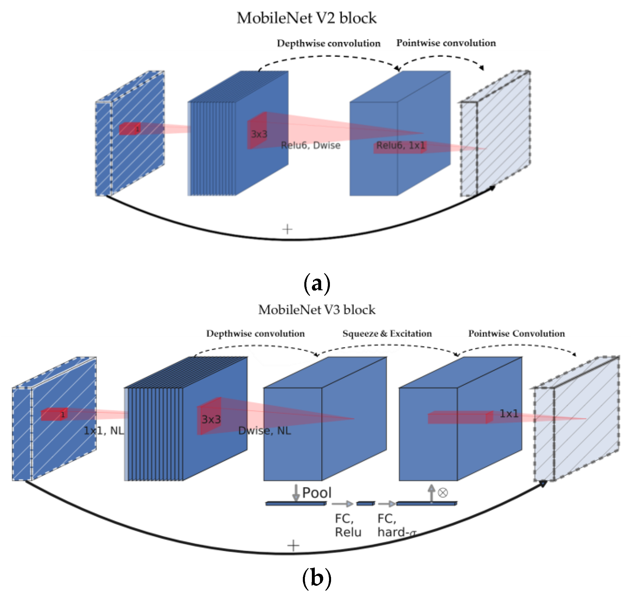
Howard et al. [20] proposed MobileNetV3, a lightweight model with improved performance compared with the previous MobileNetV2 [21] model. In this model, a building block with S&E was added to the existing bottleneck structure as shown as Figure 1, and a platform-aware neural architecture search (NAS) [22] and NetAdapt [23] were proposed to determine an efficient network structure; furthermore, layers were redesigned. Platform-aware NAS was used to optimize each block of the neural network, and NetAdapt played a role in finding optimal filter parameters by automatically fine-tuning the network created from NAS in a complementary manner to platform-aware NAS. This process helped to design an efficient network by considering the processing speed, not simply performance. By contrast, in MobileNetV3, the structure of the existing model was modified. First, the filter with a spatial resolution of 7 × 7 in the final stage was replaced with a 1 × 1 filter to obtain rich features, but with slightly more computation. This phenomenon resulted in the removal of layers that occupied a high amount of computation, which improved the structure of the final stage without deteriorating performance. Furthermore, the number of 3 × 3 filters of the existing model was reduced by half, and the activation function of the second half of the model was changed from ReLU [24] to Swish [25], which is a nonlinear function, rendering model quantization useful with a reduction in the number of calculations. This model exhibited a high level of performance and a latency of 13 to 50 ms in the classification problem using a smartphone; it also achieved a high level of performance and fast processing speed in the semantic segmentation problem for high-resolution images.

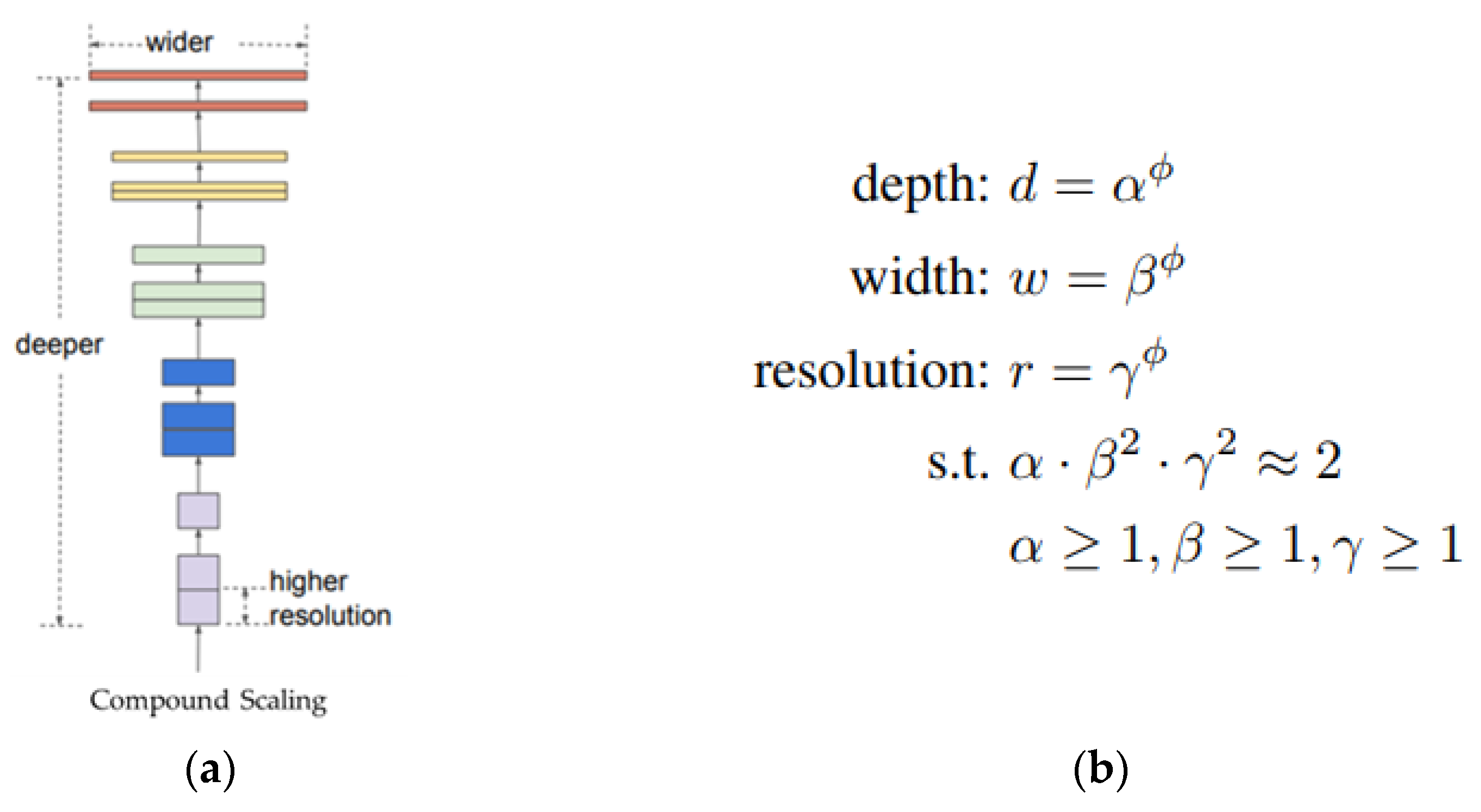
Tan et al. [26] determined the optimal combination of model depth, width, and resolution through a study on model scaling and proposed EfficientNet, which reduces model parameters. As shown as Figure 2, this study confirmed that the increase in accuracy from the increase in the depth, width, and resolution of the network rapidly decreased from a certain point; on this basis, it proposed a technique that can optimally balance depth, width, and resolution, called compound scaling. Therefore, EfficientNet, which applies compound scaling around FLOPs in a search space such as MnasNet [22], develops models up to B7 while increasing the scale (ϕ) based on the initial model B0, which enables calculations tailored to hardware specifications. The performance of the model is efficiently improved by applying techniques such as mobile inverted bottleneck and S&E. As a result of this study, EfficientNet achieved high accuracy and low computational complexity compared with existing convolution-based models with high FLOPs.

3. Methods

3.1. Model Structure

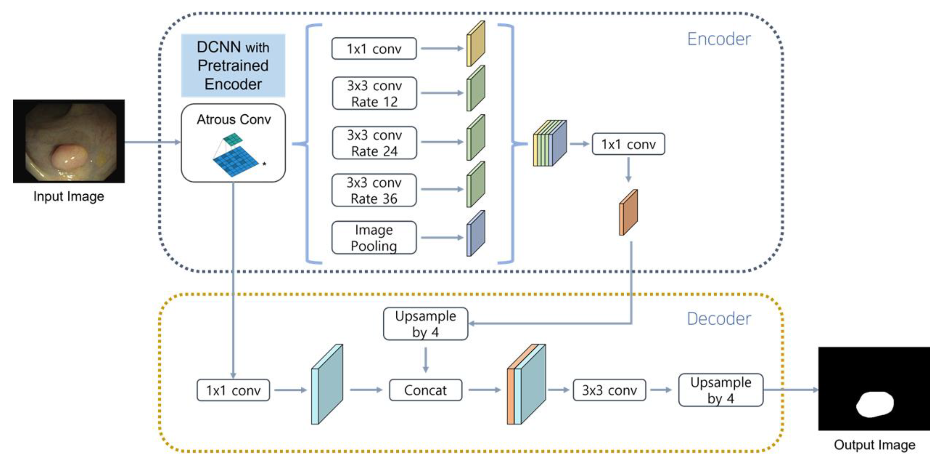
In this study, a pre-trained neural network was used as an encoder for the segmentation model. The encoder of DeepLabV3+ [27] consisted of DCNN and ASPP, in that order. In this model, DCNN played a role in compressing the information of the input data and ASPP played a role in extracting feature maps of various resolutions using the result of DCNN as an input. The pre-trained neural network received colonoscopy images as an input and played a role in extracting high-quality feature maps required by the segmentation model. This measure replaced the feature map of the encoder that the existing segmentation model had and was used as the output of the residual connection and encoder.

The decoder retained the structure of the existing segmentation model. Specifically, the structure of DeepLabV3+ was used without modification, and the decoder receiving the feature map and the result value from the encoder composed of a pre-trained neural network was trained to create a mask that was as similar as possible to the split mask of the training dataset. The model structure is displayed in Figure 3.

An efficient model suitable for segmentation of polyps was sought, and the final model was selected after performance comparison of models. Subsequently, the hyperparameters of the model were adjusted.

3.2. Experimental Details

3.2.1. Datasets

Fan et al. [28] introduced a dataset combining five polyp segmentation datasets. Each dataset has public confidence in the existing polyp segmentation task as CVC-ClinicDB [29], CVC-ColonDB [30], EndoScene [31], ETIS [32], and Kvasir [33]. Furthermore, 90% of this dataset was used as training data and the remaining 10% was used as a test dataset. In this study, the model was trained through the five-polyp segmentation dataset and the test was conducted only for CVC-ClinicDB among the existing test sets. The details of the datasets are presented in

Table 1. Metadata about polyp segmentation datasets used in the experiment.

Dataset	Resolution	Number of Patients	Number of Items
CVC-ClinicDB	384 × 288	23	612
CVC-ColonDB	500 × 574	15	300
EndoScene	500 × 574; 384 × 288	36	912
ETIS	1255 × 966	44	196
Kvasir	from 720 × 576 up to 1920 × 1072	N/A	500 images in polyp class

.

3.2.2. Loss Function

In this study, the loss functions used for training the segmentation model were binary cross-entropy (BCE) loss [34], Dice loss [35], Focal loss [36], and a combined loss function that combines these loss functions. The BCE loss is used to minimize the distribution between the predicted value and the original, which is used to increase the accuracy of each pixel by calculating the difference between the distributions for each pixel. By contrast, Dice loss is a universal division performance indicator. In the binary segmentation problem, Dice loss can be defined as a loss function that measures the similarity between masks while balancing precision and recall for the prediction mask by calculating the F1-score for the prediction and original masks. In addition to BCE and Dice loss, Focal loss is a modified version of BCE loss that down-weights the contribution of well-classified examples and focuses more on hard examples. It can improve the performance of the model in imbalanced datasets by assigning higher weights to misclassified examples. All of these loss functions have a scale between 0 and 1 and, the closer the two loss functions are to 0, the higher the similarity with the actual value. The formula for each loss is as follows:

$${Loss}_{BCE}=\left(\mathrm{y}-1\right)\mathrm{l}\mathrm{o}\mathrm{g}\left(1-\widehat{\mathrm{y}}\right)-\mathrm{y}\log \widehat{\mathrm{y}}$$

(1)

$${Loss}_{Dice}=1-\left(2\mathrm{y}\widehat{\mathrm{y}}+1\right)/\left(\mathrm{y}+\widehat{\mathrm{y}}+1\right)$$

(2)

$${Loss}_{Focal}=-\mathsf{\alpha }\mathrm{y}{\left(1-\widehat{\mathrm{p}}\right)}^{\mathsf{\gamma }}\mathrm{l}\mathrm{o}\mathrm{g}\left(\widehat{\mathrm{p}}\right)-\left(1-\mathrm{y}\right){\widehat{\mathrm{p}}}^{\mathsf{\gamma }}\mathrm{l}\mathrm{o}\mathrm{g}(1-\widehat{\mathrm{p}})$$

(3)

In the case of BCE (1), $\mathrm{y}$ denotes the actual value of each pixel and $\widehat{\mathrm{y}}$ denotes the predicted value of each pixel. In the Dice loss function (2), $\mathrm{y}$ denotes the actual mask and $\widehat{\mathrm{y}}$ denotes the predicted mask. Finally, for Focal loss (3), $\mathrm{y}$ denotes the actual value of each pixel and $\widehat{\mathrm{p}}$ denotes an estimate of the probability of the positive class, which is calculated based on the predicted value. The focusing parameter, γ, determines the extent to which highly confident and accurate predictions contribute to the overall loss function. Finally, the hyperparameter α plays a crucial role in balancing precision and recall by adjusting the weighting of errors for the positive class. Specifically, the value of α determines the degree to which errors for the positive class are penalized or rewarded, thus affecting the overall performance of the model.

3.2.3. Experimental Details

In this study, the pytorch [37] framework was used for training and testing of the model, and all training processes were performed on an i7-10700F with an RTX 2060 super 8GB graphics card. To prevent model overfitting, the dataset was divided into 80% training data, 10% validation data, and 10% test data. Besides, the model image was resized to 288 × 384, the size of the CVC-ClinicDB dataset for testing. Finally, to ensure fairness in the model learning process, each model in our experiments was trained on eight different training/validation partitions that were generated from distinct random seeds. The reported results are the average of the aggregated performance metrics across all partitions.

Meanwhile, there are some differences in experimental details in the model exploration process and the hyperparameter tuning process. AdamW [38] was used as the optimizer for the model learning [36]. In this model, the learning rate is set to 1 × 10⁻³ and the weight reduction rate was set to 1 × 10⁻² to determine the optimal minima while minimizing the divergence of the loss function. Next, in the case of models to be used as encoders (MobileNetV3, EfficientNet, and RegNet), pre-training was performed on the ImageNet dataset. Besides, the number of training iterations was set to 1000 and the patience for early stopping of training was set to 50 to extract the maximum accuracy from the model. Finally, the Gaussian noise, flip, and coarse dropout [39] augmentation techniques were applied through the Albumentation [40] library.

On the other hand, in the hyperparameter tuning process, the number of training iterations was set to 100 and patience was set to 15 to evaluate the influence of the hy-perparameters quickly and fairly; training was conducted excluding the Gaussian noise technique included in the selection process. Finally, optimizers were defined as hyperparameters and performance was compared to various optimizers after model adoption. The details of the experimental environment are presented in

Table 2. Experiment details for model training.

Training Environments	Model Comparison	Hyperparameter Tuning
Hardware	i7-10700F, 32GB RAM, RTX 2060 super 8GB
Optimizers	AdamW (Learning rate: 1 × 10−3, weight decay: 1 × 10−2)	AdamW, AdamP [41], DiffGrad [42], Ranger [43], SGDW, and Yogi [44]
Image resolution	288 × 384
Pre-trained dataset	ImageNet
Epoch	1000	100
Patience	50	15
Data augmentation	Gaussian Noise (p = 0.3), HorizontalFlip (p = 0.3), VerticalFlip (p = 0.3), CoarseDropout (max_holes = 8, max_height = 10, max_width = 10, fill_value = 0, p = 0.2)	HorizontalFlip (p = 0.3), VerticalFlip (p = 0.3), CoarseDropout (max_holes = 8, max_height = 10, max_width = 10, fill_value = 0, p = 0.2)

.

4. Results

4.1. Model Exploration for Polyp Segmentation Models

To create a polyp segmentation model with fast processing speed, this study proposed a segmentation and an encoder model with a high level of performance while maximizing computational efficiency. In the case of the segmentation model, U-Net and DeepLabV3+, which exhibit a faster processing speed and superior performance in segmenting medical images than other models, were used as test subjects.

In the encoder, the scope is limited to CNN-based models instead of transformer-based models because transformer modules have a large amount of computation and the global feature map generated by the model makes it difficult to consider detailed information in the decoder stage, requiring a large amount of computation to compensate for this. In this study, the standard of the lightweight model was set as the number of parameters of 10 M; as a result, MobileNetV3, EfficientNet, and RegNet [45] were selected as target encoders. Information on these models can be obtained in

Table 3. Information on models selected as encoders. Top1-acc has the same meaning as accuracy and is based on the ImageNet dataset.

Models	Detailed Model	Parameters (M)	Top1-acc
MobileNetV3	MobileNetV3-L 0.75	4.0	73.3%
EfficientNet	EfficientNet-B3	10.0	81.6%
RegNet	RegNetY-1.6GF	6.3	76.3%

.

4.2. Comparison of Polyp Models

Table 4. Results for comparison experiments between models. The term “Val Dice” refers to the average Dice score obtained by validating the model on the validation dataset, following eight training iterations. The bolded values indicate the highest level of performance for each respective metric.

Method	Val Dice (%)	Test Dice (%)	Parameters (M)	GFLOPs
U-Net (MobileNetV3)	93.42	92.45	18.64	4.795
U-Net (EfficientNet)	92.01	90.86	33.88	6.278
U-Net (RegNet)	91.56	89.51	55.27	8.808
DeepLabV3+ (MobileNetV3)	94.03	92.23	6.18	1.623
DeepLabV3+ (EfficientNet)	93.75	92.73	28.25	4.351
DeepLabV3+ (RegNet)	93.21	92.05	45.61	5.718

presents the results of the experiment in the environment in which the selected model and encoder were proposed. The performance between the models was compared to the complexity of the models through the Dice coefficient to consider the accuracy, the number of parameters that can quantify the degree of light weight of the model, and the GFLOPs index. Parameters are variables of deep learning models and, as the number increases, more complex problems can be solved. In the case of FLOPs, the number of floating-point operations required to execute the model indicates the sum of addition and multiplication operations theoretically performed in the model.

In terms of accuracy, U-Net and DeepLabV3+ exhibited satisfactory performance. DeepLabV3+ achieved a Dice coefficient of 92% or more in all encoders, which revealed robustness to changes in encoders. In the case of U-Net, the deviation according to the encoder was not small, which revealed the disadvantage of low learning stability. In terms of the number of parameters and the amount of computation, the MobileNetV3 model has significant advantages over other lightweight models when used as an encoder. In terms of accuracy, MobileNetV3 revealed comparable performance to models using EfficientNet, which proved its competitiveness. Therefore, in this experiment, DeepLabV3+ was adopted as the segmentation model and MobileNetV3 was adopted as the pre-learning encoder.

4.3. Hyperparameter Tuning

In the experimental model composed of MobileNetV3 and DeepLabV3+, the output stride, decoder channel, and atrous rate are defined as key variables. Furthermore, the loss function and optimizer in the learning process can affect the learning performance of the model and are thus also included in the experiment. In this experiment, the influence of the features was observed by comparing the performance while adjusting the value of each hyperparameter, and the correlation between features was subsequently observed through the combination of each feature. Finally, a model with improved performance was proposed.

4.3.1. Output Stride

The output stride is the size difference between the input image and the final feature map of the encoder and is a hyperparameter that can determine the amount of information compression. In this study, the performance was compared by reducing the basic factor from 16 to 8 times, but, as shown in

Table 5. Performance comparison for the output stride. The bolded values indicate the highest level of performance for each respective metric.

Output Stride	Val Dice (%)	Test Dice (%)	GFLOPs
8	90.89	90.97	4.220
16 (Baseline)	91.72	91.86	1.623

, also reducing the output stride degraded model performance. This is because accurate segmentation is difficult because of the inability to compress information for segmentation in cases in which regional information is crucial. Therefore, the polyp boundary may not be precisely formed or the polyp may not be properly recognized. Furthermore, as the size of the image to be processed by the model doubled, the amount of computation increased by more than two times, indicating that this variable is not suitable for a real-time polyp segmentation model.

4.3.2. Decoder Channel

The decoder channel is the number of convolution filters of the ASPP module and is adjusted to determine the density of the information of the final feature map of the ASPP module. However, in the case of this hyperparameter, accuracy can be increased, but the amount of calculation increases as well; therefore, setting it appropriately is critical. In this experiment, we determined the optimal number of kernels by comparing the basic parameter of 256 and 196, 288, and 384 channels. In terms of the prediction mask, the model trained with the basic channel and 288 decoder channels accurately captured the border and pattern of polyps, but the quality of the segmentation images was relatively low owing to the lack of information in 196 cases. Furthermore, in the case of 388 cases, the variance of the feature map was too high; thus, uniform segmentation quality was not observed. The results are presented in

Table 6. Performance comparison for decoder channels. The bolded values indicate the highest level of performance for each respective metric.

Decoder Channel	Val Dice (%)	Test Dice (%)	GFLOPs
256 (Baseline)	91.72	91.86	1.623
196	92.09	91.96	1.260
288	92.24	92.27	1.845
384	92.22	91.60	2.628

.

4.3.3. Atrous Rate

The atrous rate denotes the interval of atrous convolution within the model. DeepLabV3+ has three atrous convolution blocks for spatial pyramid pooling; therefore, the parameter must also be set to three integers. The point of attention in this experiment was the increase in segmentation performance for small polyps, which could be attributed to the fact that the existing model did not exhibit suitable performance for small polyps. This process was evaluated through comparison between images instead of quantitative evaluation. The basic ratio was 12/24/36 and the experimental parameters were 8/16/32 and 8/22/36; when adjusting the interval scale, it was tested whether both large and small polyps could be divided well. In the quantitative evaluation of model performance, parameters of 8/22/36 demonstrated the best performance, and the amount of computation was maintained when reducing the atrous rate. An image comparison of this experiment clearly revealed the difference. When the atrous rate was lowered to 8/16/32, precise segmentation was possible for small polyps, but the limitation of not capturing the shape of polyps in large polyps was revealed. In the case of an atrous rate of 8/22/32, small polyps were captured better than in the existing model, and although a loss of contextual information was observed in large polyps, a segmentation mask was created that preserved the information well compared with that of 8/16/32 The results are presented in

Table 7. Performance comparison for the atrous rate. The bolded values indicate the highest level of performance for each respective metric.

Atrous Rate	Val Dice (%)	Test Dice (%)	GFLOPs
12/24/36 (Baseline)	91.72	91.86	1.623
8/16/32	91.07	90.80	1.623
8/22/36	92.59	92.12	1.623

.

4.3.4. Loss Function

The loss function is a function that defines the error between the predicted and ground truth during model training. In the case of the loss function, because the result of the model can change depending on the design point of view, it is a significant variable that can change the performance of the model depending on the definition of the formula. The loss function in the segmentation problem is divided into a distribution-based function, a region-based function, and a boundary-based function. Among these functions, the most widely used ones are the distribution-based cross-entropy and focal functions and the region-based Dice function.

In this experiment, we compared the performance of BCE loss, Dice loss, Dice + Focal loss, and BCE + Dice loss, which recorded good performance in the study proposed by Ma et al. [46]. When the two loss functions were combined, the experiment was conducted without weighting. The results are presented in

Table 8. Performance comparison for the loss function. The bolded values indicate the highest level of performance for each respective metric.

Loss Function	Val Dice (%)	Test Dice (%)	GFLOPs
BCE + Dice (baseline)	91.72	91.86	1.623
BCE	91.15	90.59	1.623
Dice	91.63	91.76	1.623
Dice + Focal	92.19	91.86	1.623

.

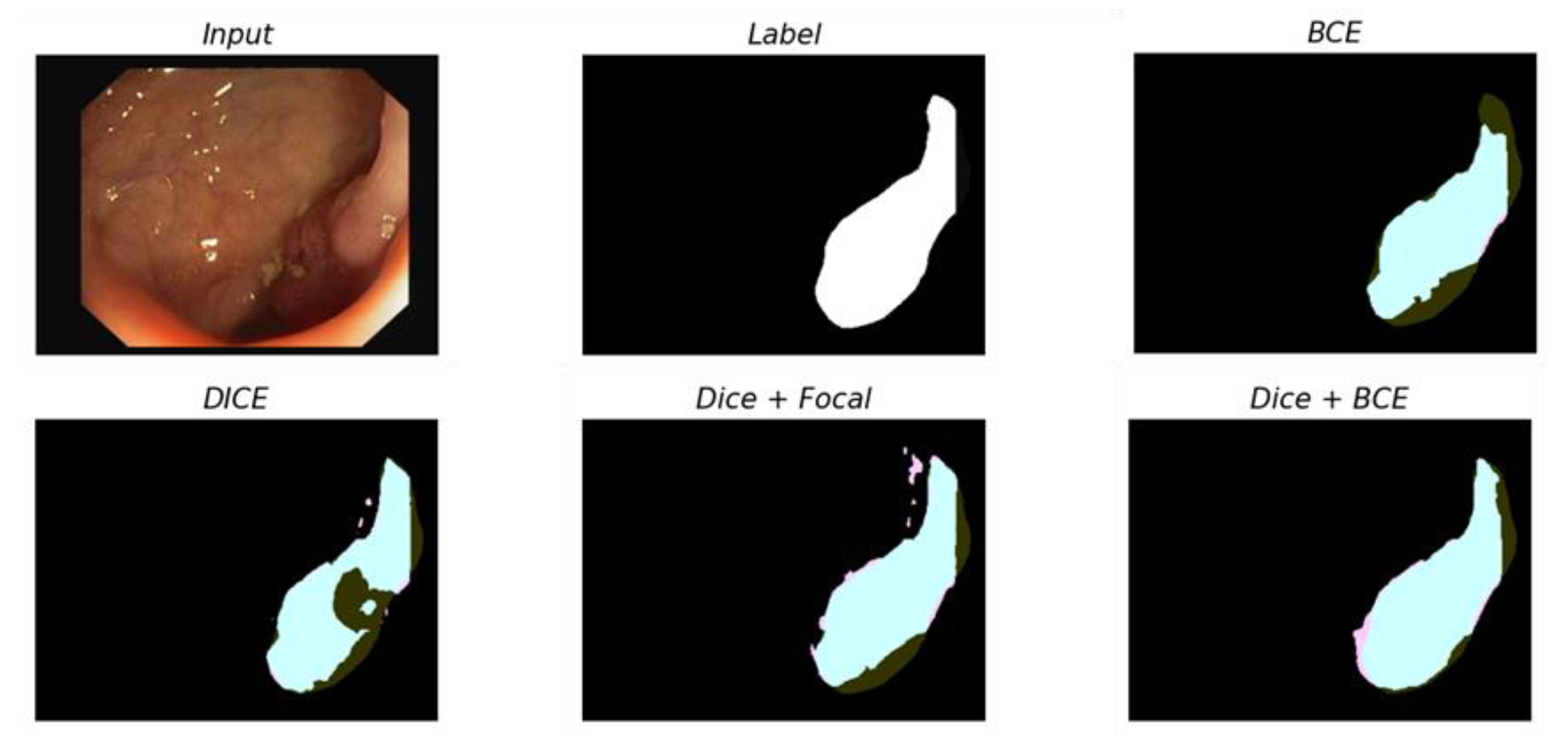
All models showed similar or identical accuracy, except for BCE, and the amount of computation did not differ. However, in the prediction mask, the difference in the loss function could be confirmed. In the case of BCE function, the predictive mask itself was dense, but it did not accurately capture the overall shape of the polyps; this disadvantage has been highlighted especially for large polyps. The Dice function found the polyp area well, but demonstrated poor performance in terms of localization. In the case of the loss function, by adding the Dice and Focal functions, the shape of the polyp was found accurately and the border was well segmented; however, polyp detection often occurred in areas other than polyps, which indicated the risk of false positives. By contrast, the loss function using BCE and Dice could overcome all of these limitations. As shown in prediction masks, this loss function has a complementary role between the BCE and Dice functions; thus, both global context and local information can be properly utilized. Unlike the Dice + focal function, it is also confirmed that there are almost no false positive pixels.

4.3.5. Optimizers

The optimizer is used to find parameters that minimize the loss function in training and is a critical hyperparameter in determining model performance. Stochastic gradient descent (SGD) [47], Adam [48], and Nesterov accelerated gradient are widely used optimizers [49]. Various optimizers developed from these models exhibit a faster learning speed and higher optimization performance than existing functions. In this study, based on the visualization of learning strategies for multiple optimizers conducted by Novik et al. [50,51,52], five optimizers with optimal learning strategies were selected. AdamW, AdamP, DiffGrad, Ranger, SGDW, and Yogi were tested in our experiment, and the experimental results are presented in

Table 9. Performance comparison for optimizers. The bolded values indicate the highest level of performance for each respective metric.

Optimizers	Val Dice (%)	Test Dice (%)	GFLOPs
AdamW (baseline)	91.72	91.86	1.623
AdamP	92.07	91.31	1.623
DiffGrad	92.97	92.41	1.623
Ranger	94.95	93.18	1.623
SGDW	57.21	28.41	1.623
Yogi	90.67	90.84	1.623

.

Among all optimizers, Ranger exhibited the best performance, achieving an accuracy higher than 93%. This optimizer, together with DiffGrad, reduced the loss in the training phase at a very high speed, and its learning efficiency was also high. By contrast, in the case of SGDW, proper learning was impossible because of the divergence of the loss function during the training phase. For segmented images generated by each model, it was found that all optimizers except SGDW preserved the global context, but AdamW, DiffGrad, and Ranger achieved precise results in terms of localization. In particular, for the Ranger optimizer, the quality of the mask significantly improved because almost no false positive pixels were observed compared with other functions.

4.4. Final Model Selection

The optimal model for the real-time segmentation of polyps in colonoscopy images was found and its hyperparameters were adjusted to minimize the increase in computational complexity while improving performance. In this experiment, a novel model with optimal performance was proposed through ablation study. First, the BCE + Dice loss function and Ranger optimizer, which revealed a significant performance improvement in previous experiments, were applied to the model. Next, experiments were conducted on the combination of decoder channel and atrous rate to compare the performance of the three cases.

For this experiment, the number of iterations and patience were changed to 1000 and 50, respectively, in the same environment as the hyperparameter adjustment process. These parameters were set to accurately capture polyps by optimizing the model to the data. The experimental results, as shown in

Table 10. Results of ablation study for final model selection. The bolded values indicate the highest level of performance for each respective metric.

Method	Val Dice (%)	Test Dice (%)	GFLOPs
DeepLabV3+ + MobileNetV3 (Baseline)	94.03	92.23	1.623
Ranger + decoder channel	95.83	93.52	1.845
Ranger + atrous rate	96.35	93.79	1.623
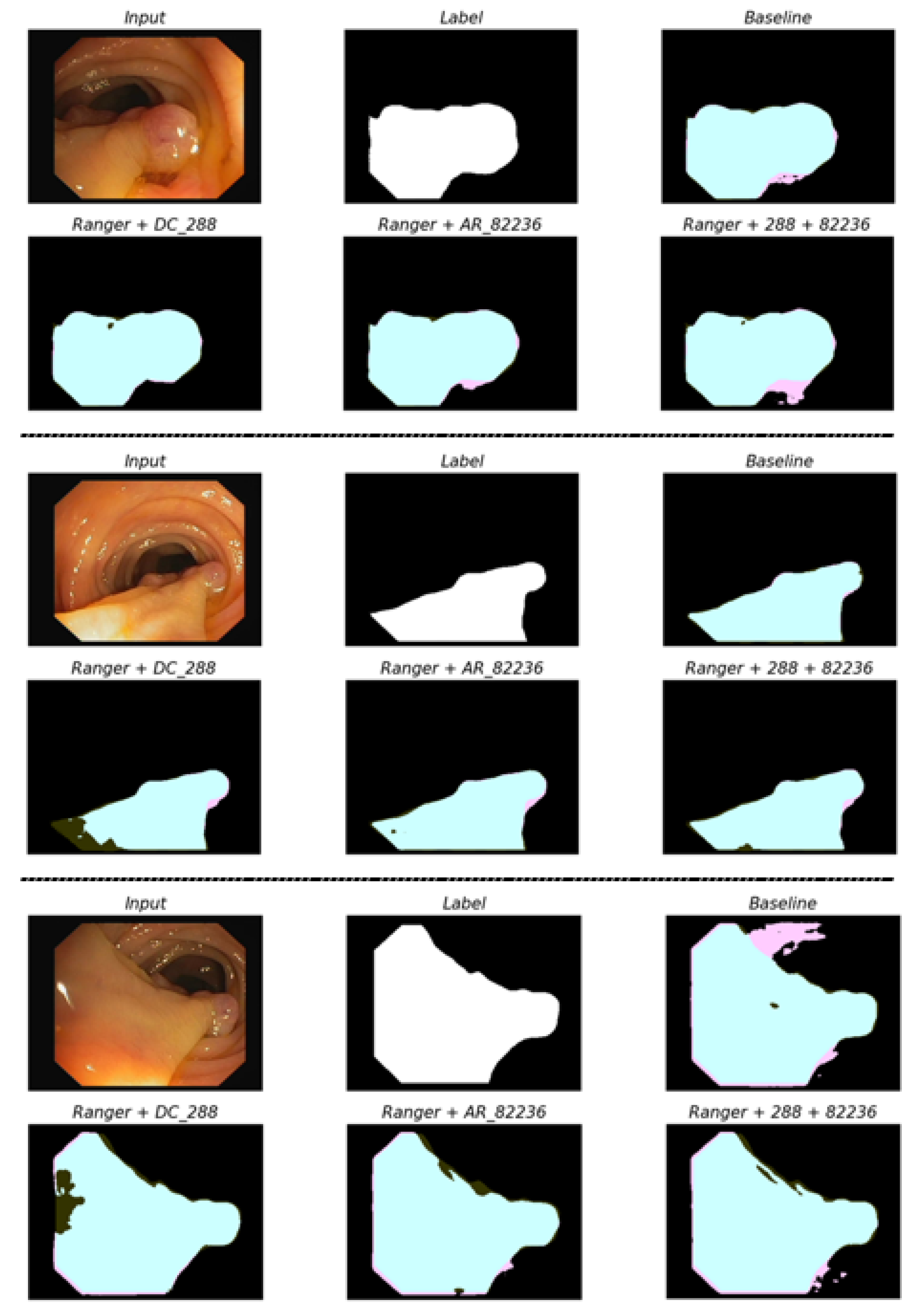
Ranger + atrous rate + decoder channel	96.21	93.24	1.845

, are supported by the visual comparisons of images between the models in Figure 4. Contrary to expectations, accuracy was highest when only the atrous rate was adjusted. When the atrous rate and the decoder channel were simultaneously adjusted, the performance degraded compared with individual adjustments. This phenomenon can be interpreted as a conflicting problem between the reduction in the atrous rate, which increases the localization quality of the small size of the model, and the increase in the decoder channel, which can deteriorate the localization quality by increasing the variance of model parameters.

When considering the segmentation mask, as shown in Figure 5, all three models exhibited higher localization performance and global performance than the basic model for the resulting mask in most images. However, in the case of the decoder channel, the quality was low in terms of localization instead of generating the boundary as similar as possible to the label. When the atrous rate was adjusted, the boundary was more unstable than that of other models and a hole occurred in the polyp mask. However, both the shape and detail of the polyp were captured effectively. Finally, when both parameters were adjusted, the disadvantages of the two models were compensated for in some cases; however, in the case of some polyps, the quality was slightly degraded. This phenomenon can be determined to be a poor approach in terms of stability compared with using the two parameters individually.

This experiment confirmed that the model adjusted for the atrous rate exhibited high accuracy and almost no degradation in speed. Therefore, in this study, the model adjusted for the atrous rate was selected as the final model.

5. Discussion

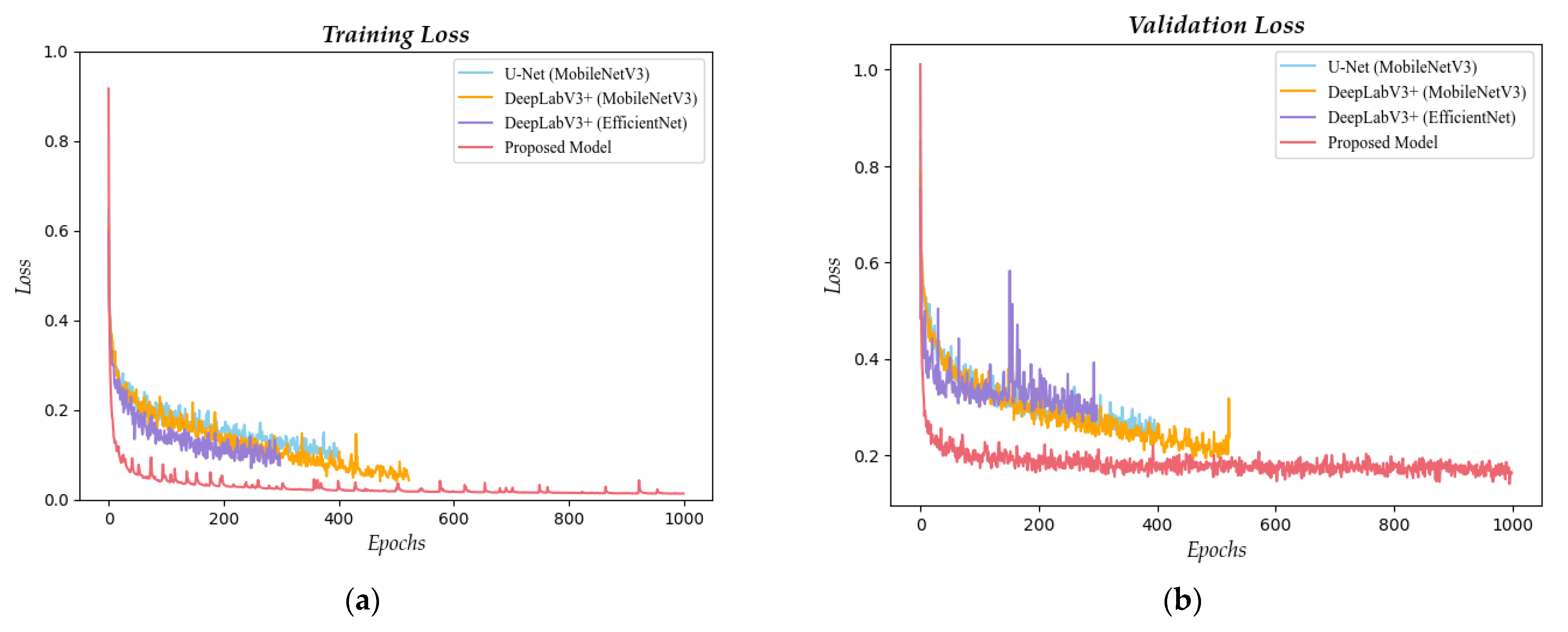
In this study, model search and selection, hyperparameter tuning, and final model adoption were performed to create a model with a high level of performance and a fast processing speed. The modified DeepLabV3+ model using MobileNetV3 as an encoder revealed a Dice coefficient of 93.79% and an operation amount of 1.623 GFLOPs in the CVC-ClinicDB dataset; the comparison between other models proved that the model exhibited reasonable performance in both processing speed and accuracy. Also, As shown in Figure 6, our proposed model converged faster and achieved lower loss compared to the previous models. This model improved accuracy by nearly 2% compared to the TransFuse-S model and reduced the computational amount by 180 times; this indicates that complicating the model is not the correct approach to improving accuracy.

Table 11. Performance comparison of proposed and existing models on CVC-ClinicDB.

Method	Test Dice (%)	Parameters (M)	GFLOPs
TransFuse-S	91.80	26.30	286.36
ResUNet++ + CRF	92.03	4.07	26.668
DoubleUNet	92.39	29.29	91.052
HarDNet-MSEG	93.20	66.47	1.017
MSRFNet	94.20	18.38	158.116
SSFormer	94.47	66.20	25.224
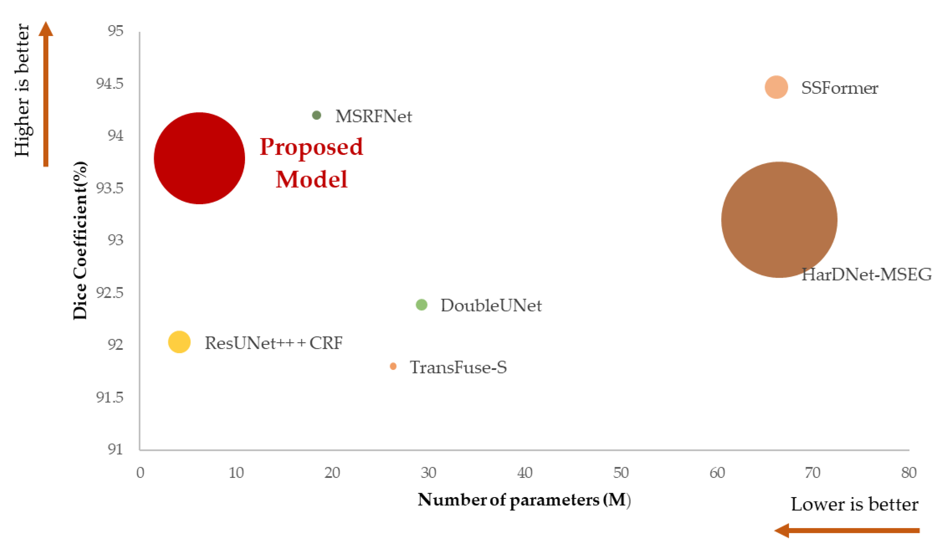
Proposed Model	93.79	6.18	1.623

presents a comparison of the performance of the proposed model to that of the existing model.

Colonoscopy is a screening tool optimized for observing and removing polyps. However, distinguishing polyps using the naked eye is difficult in several cases; therefore, the polyp area should be segmented using morphological information in addition to location and size information. The lightweight segmentation model proposed in this study can solve these tasks in real time in real medical settings and is expected to be a screening algorithm with a comparative advantage over object detection methods based on high accuracy.

However, in this study, distinguishing cases where polyps do not exist is not possible, as the dataset does not contain data with no polyps; this may cause a problem of false positive detection of polyp regions even when no polyps exist. This model also exhibited poor performance in accurately segmenting all polyp patterns, and its applicability in a limited environment by learning and inferring a model for still images through a graphical processing unit remains unclear.

6. Conclusions

The model developed in this study balances high accuracy and fast processing speed, focusing on a polyp segmentation model that can be used in real time. The results of the study revealed that increasing the complexity and amount of computation of the model to increase existing accuracy may not be effective. We tried to prove that a high level of performance can be achieved even with a low amount of computation and model scale by combining existing lightweight models and optimizing them. DeepLabV3+ was used as a split model and MobileNetV3 as an encoder, achieving a high level of performance of 92.23% Dice coefficient, 1.623 GFLOPs operation amount, and 6.18 M parameters in the CVC-ClinicDB dataset. After adjusting the parameters, the amount of computation and model parameters were maintained, the Dice coefficient was increased to 93.79%, and a faster and more precise segmentation model was proposed than the existing model as shown in Figure 7.

In the future, to overcome the mentioned limitations, the following follow-up studies are suggested. The specificity of the execution speed and false positives in the colonoscopy video should be verified through the image data, including integrating images without polyps into the training data. To verify whether the lightweight split model can be run in harsh environments through CPU testing, studies should also be conducted to improve generalization performance and optimize models that maintain real-time properties and loss functions.

References

- Sawicki, T.; Ruszkowska, M.; Danielewicz, A.; Niedźwiedzka, E.; Arłukowicz, T.; Przybyłowicz, K.E. A review of colorectal cancer in terms of epidemiology, risk factors, development, symptoms and diagnosis. Cancers 2021, 13, 2025. [Google Scholar] [CrossRef] [PubMed]
- Sohn, D.K.; Kim, M.J.; Park, Y.; Suh, M.; Shin, A.; Lee, H.Y.; Im, J.P.; Cho, H.-M.; Hong, S.P.; Kim, B.-H.; et al. The Korean guideline for colorectal cancer screening. J. Korean Med. Assoc. 2015, 58, 420. [Google Scholar] [CrossRef]
- Baxter, N.N. Association of Colonoscopy and Death from colorectal cancer. Ann. Intern. Med. 2009, 150, 1. [Google Scholar] [CrossRef] [PubMed]
- Chen, C.; Zhou, K.; Wang, Z.; Xiao, R. Generative consistency for semi-supervised cerebrovascular segmentation from TOF-MRA. IEEE Trans. Med. Imaging 2023, 42, 346–353. [Google Scholar] [CrossRef] [PubMed]
- Wu, Q.; Chen, Y.; Huang, N.; Yue, X. Weakly-supervised cerebrovascular segmentation network with shape prior and model indicator. In Proceedings of the 2022 International Conference on Multimedia Retrieval, Newark, NJ, USA, 27–30 June 2022. [Google Scholar]
- Isensee, F.; Jaeger, P.F.; Kohl, S.A.; Petersen, J.; Maier-Hein, K.H. NNU-net: A self-configuring method for deep learning-based biomedical image segmentation. Nat. Methods 2020, 18, 203–211. [Google Scholar] [CrossRef]
- Jha, D.; Smedsrud, P.H.; Riegler, M.A.; Johansen, D.; Lange, T.D.; Halvorsen, P.; Johansen, H.D. ResUNet++: An Advanced Architecture for Medical Image Segmentation. In Proceedings of the 2019 IEEE International Symposium on Multimedia (ISM), San Diego, CA, USA, 9–11 December 2019. [Google Scholar]
- Ronneberger, O.; Fischer, P.; Brox, T. U-Net: Convolutional Networks for Biomedical Image Segmentation. In Proceedings of the Medical Image Computing and Computer-Assisted Intervention–MICCAI 2015: 18th International Conference, Munich, Germany, 5–9 October 2015; Springer International Publishing: Cham, Switzerland, 2015; pp. 234–241. [Google Scholar]
- Hu, J.; Shen, L.; Sun, G. Squeeze-and-excitation networks. In Proceedings of the 2018 IEEE/CVF Conference on Computer Vision and Pattern Recognition, Salt Lake City, UT, USA, 18–23 June 2018. [Google Scholar]
- Li, H.; Xiong, P.; An, J.; Wang, L. Pyramid Attention Network for semantic segmentation. arXiv 2018. [Google Scholar] [CrossRef]
- He, K.; Zhang, X.; Ren, S.; Sun, J. Deep residual learning for image recognition. In Proceedings of the 2016 IEEE Conference on Computer Vision and Pattern Recognition (CVPR), Las Vegas, NV, USA, 27 June–30 June 2016. [Google Scholar]
- Jha, D.; Smedsrud, P.H.; Johansen, D.; de Lange, T.; Johansen, H.D.; Halvorsen, P.; Riegler, M.A. A comprehensive study on colorectal polyp segmentation with resunet++, conditional random field and test-time augmentation. IEEE J. Biomed. Health Inform. 2021, 25, 2029–2040. [Google Scholar] [CrossRef]
- Lafferty, J.D.; Profile, V.; McCallum, A.; Pereira, F.C.N.; Metrics, O.M.V.A. Conditional random fields. In Proceedings of the Eighteenth International Conference on Machine Learning, San Francisco, CA, USA, 28 June–1 July 2001; Available online: https://dl.acm.org/doi/10.5555/645530.655813 (accessed on 15 March 2023).
- Shanmugam, D.; Blalock, D.; Balakrishnan, G.; Guttag, J. Better aggregation in test-time augmentation. In Proceedings of the 2021 IEEE/CVF International Conference on Computer Vision (ICCV), Montreal, QC, Canada, 10–17 October 2021. [Google Scholar]
- Srivastava, A.; Jha, D.; Chanda, S.; Pal, U.; Johansen, H.; Johansen, D.; Riegler, M.; Ali, S.; Halvorsen, P. MSRF-net: A multi-scale residual fusion network for Biomedical Image Segmentation. IEEE J. Biomed. Health Inform. 2022, 26, 2252–2263. [Google Scholar] [CrossRef]
- Sun, J.; Darbehani, F.; Zaidi, M.; Wang, B. Saunet: Shape attentive U-net for interpretable medical image segmentation. In Proceedings of the Medical Image Computing and Computer Assisted Intervention—MICCAI 2020, Lima, Peru, 4–8 October 2020; pp. 797–806. [Google Scholar]
- Zhang, Y.; Liu, H.; Hu, Q. Transfuse: Fusing transformers and cnns for medical image segmentation. In Proceedings of the Medical Image Computing and Computer Assisted Intervention—MICCAI 2021, Strasbourg, France, 27 September–1 October 2021; pp. 14–24. [Google Scholar]
- Wang, J.; Huang, Q.; Tang, F.; Meng, J.; Su, J.; Song, S. Stepwise feature fusion: Local guides global. In Proceedings of the Medical Image Computing and Computer Assisted Intervention–MICCAI 2022: 25th International Conference, Singapore, 18–22 September 2022; Springer Nature: Cham, Switzerland, 2022; pp. 110–120. [Google Scholar]
- Wang, W.; Xie, E.; Li, X.; Fan, D.-P.; Song, K.; Liang, D.; Lu, T.; Luo, P.; Shao, L. PVT V2: Improved baselines with pyramid vision transformer. Comput. Vis. Media 2022, 8, 415–424. [Google Scholar] [CrossRef]
- Howard, A.; Sandler, M.; Chen, B.; Wang, W.; Chen, L.-C.; Tan, M.; Chu, G.; Vasudevan, V.; Zhu, Y.; Pang, R.; et al. Searching for MobileNetV3. In Proceedings of the 2019 IEEE/CVF International Conference on Computer Vision (ICCV), Seoul, Republic of Korea, 27 October–2 November 2019. [Google Scholar]
- Sandler, M.; Howard, A.; Zhu, M.; Zhmoginov, A.; Chen, L.-C. MobileNetV2: Inverted residuals and linear bottlenecks. In Proceedings of the 2018 IEEE/CVF Conference on Computer Vision and Pattern Recognition, Salt Lake City, UT, USA, 18–22 June 2018. [Google Scholar]
- Tan, M.; Chen, B.; Pang, R.; Vasudevan, V.; Sandler, M.; Howard, A.; Le, Q.V. MnasNet: Platform-aware neural architecture search for mobile. In Proceedings of the 2019 IEEE/CVF Conference on Computer Vision and Pattern Recognition (CVPR), Long Beach, CA, USA, 15–20 June 2019. [Google Scholar]
- Yang, T.-J.; Howard, A.; Chen, B.; Zhang, X.; Go, A.; Sandler, M.; Sze, V.; Adam, H. NetAdapt: Platform-aware neural network adaptation for mobile applications. In Proceedings of the European Conference on Computer Vision (ECCV), Munich, Germany, 8–14 September 2018; pp. 289–304. [Google Scholar]
- Agarap, A.F. Deep learning using rectified linear units (ReLU). arXiv 2018. [Google Scholar] [CrossRef]
- Ramachandran, P.; Zoph, B.; Le, Q.V. Searching for activation functions. arXiv 2017. [Google Scholar] [CrossRef]
- Tan, M.; Le, Q. Efficient Net: Rethinking Model Scaling for Convolutional Neural Networks. 2019. Available online: https://proceedings.mlr.press/v97/tan19a.html (accessed on 15 March 2023).
- Chen, L.-C.; Zhu, Y.; Papandreou, G.; Schroff, F.; Adam, H. Encoder-decoder with atrous separable convolution for Semantic Image segmentation. In Proceedings of the European Conference on Computer Vision (ECCV), Munich, Germany, 8–14 September 2018; pp. 833–851. [Google Scholar]
- Fan, D.-P.; Ji, G.-P.; Zhou, T.; Chen, G.; Fu, H.; Shen, J.; Shao, L. PraNet: Parallel reverse attention network for polyp segmentation. In Proceedings of the Medical Image Computing and Computer Assisted Intervention—MICCAI 2020, Lima, Peru, 4–8 October 2020; pp. 263–273. [Google Scholar]
- Bernal, J.; Sánchez, F.J.; Fernández-Esparrach, G.; Gil, D.; Rodríguez, C.; Vilariño, F. WM-Dova Maps for accurate polyp highlighting in colonoscopy: Validation vs. saliency maps from physicians. Comput. Med. Imaging Graph. 2015, 43, 99–111. [Google Scholar] [CrossRef] [PubMed]
- Tajbakhsh, N.; Gurudu, S.R.; Liang, J. Automated polyp detection in colonoscopy videos using shape and context information. IEEE Trans. Med. Imaging 2016, 35, 630–644. [Google Scholar] [CrossRef] [PubMed]
- Vázquez, D.; Bernal, J.; Sánchez, F.J.; Fernández-Esparrach, G.; López, A.M.; Romero, A.; Drozdzal, M.; Courville, A. A benchMarchk for endoluminal scene segmentation of colonoscopy images. J. Healthc. Eng. 2017, 2017, 1–9. [Google Scholar] [CrossRef] [PubMed]
- Silva, J.; Histace, A.; Romain, O.; Dray, X.; Granado, B. Toward embedded detection of polyps in WCE images for early diagnosis of colorectal cancer. Int. J. Comput. Assist. Radiol. Surg. 2013, 9, 283–293. [Google Scholar] [CrossRef]
- Jha, D.; Smedsrud, P.H.; Riegler, M.A.; Halvorsen, P.; de Lange, T.; Johansen, D.; Johansen, H.D. Kvasir-SEG: A segmented polyp dataset. In MultiMedia Modeling, Proceedings of the 26th International Conference, MMM 2020, Daejeon, South Korea, 5–8 January 2020; Proceedings, Part II; Springer International Publishing: Cham, Switzerland, 2019; Volume 11962, pp. 451–462. [Google Scholar]
- Ma, Y.-D.; Liu, Q.; Quan, Z. Automated image segmentation using improved PCNN model based on cross-entropy. In Proceedings of the 2004 International Symposium on Intelligent Multimedia, Video and Speech Processing, Hong Kong, China, 20–22 October 2004. [Google Scholar]
- Sudre, C.H.; Li, W.; Vercauteren, T.; Ourselin, S.; Jorge Cardoso, M. Generalised dice overlap as a deep learning loss function for highly unbalanced segmentations. In Proceedings of the Deep Learning in Medical Image Analysis and Multimodal Learning for Clinical Decision Support, Québec City, QC, Canada, 14 September 2017; pp. 240–248. [Google Scholar]
- Lin, T.-Y.; Goyal, P.; Girshick, R.; He, K.; Dollar, P. Focal loss for dense object detection. IEEE Trans. Pattern Anal. Mach. Intell. 2020, 42, 318–327. [Google Scholar] [CrossRef]
- Paszke, A.; Gross, S.; Massa, F.; Lerer, A.; Bradbury, J.; Chanan, G.; Killeen, T.; Lin, Z.; Gimelshein, N.; Antiga, L.; et al. Pytorch: An Imperative Style, High-Performance Deep Learning Library. Available online: https://papers.nips.cc/paper/9015-pytorch-an-imperative-style-high-performance-deep-learning-library (accessed on 15 March 2023).
- Loshchilov, I.; Hutter, F. Decoupled weight decay regularization. arXiv 2017. [Google Scholar] [CrossRef]
- DeVries, T.; Taylor, G.W. Improved regularization of convolutional neural networks with cutout. arXiv 2017. [Google Scholar] [CrossRef]
- Buslaev, A.; Iglovikov, V.I.; Khvedchenya, E.; Parinov, A.; Druzhinin, M.; Kalinin, A.A. Albumentations: Fast and flexible image augmentations. Information 2020, 11, 125. [Google Scholar] [CrossRef]
- Heo, B.; Chun, S.; Oh, S.J.; Han, D.; Yun, S.; Kim, G.; Uh, Y.; Ha, J.-W. Adamp: Slowing down the slowdown for momentum optimizers on scale-invariant weights. arXiv 2020. [Google Scholar] [CrossRef]
- Dubey, S.R.; Chakraborty, S.; Roy, S.K.; Mukherjee, S.; Singh, S.K.; Chaudhuri, B.B. Diffgrad: An optimization method for Convolutional Neural Networks. IEEE Trans. Neural Netw. Learn. Syst. 2020, 31, 4500–4511. [Google Scholar] [CrossRef] [PubMed]
- Lessw2020 Lessw2020/Ranger-Deep-Learning-Optimizer: Ranger—A Synergistic Optimizer Using Radam (Rectified Adam), Gradient Centralization and Lookahead in one Codebase. Available online: https://github.com/lessw2020/Ranger-Deep-Learning-Optimizer (accessed on 15 March 2023).
- Zaheer, M.; Reddi, S.; Sachan, D.; Kale, S.; Kumar, S. Adaptive methods for nonconvex optimization. Adv. Neural Inf. Process. Syst. 2018, 31, 9815–9825. [Google Scholar]
- Radosavovic, I.; Kosaraju, R.P.; Girshick, R.; He, K.; Dollar, P. Designing network design spaces. In Proceedings of the 2020 IEEE/CVF Conference on Computer Vision and Pattern Recognition (CVPR), Seattle, WA, USA, 13–19 June 2020. [Google Scholar]
- Ma, J.; Chen, J.; Ng, M.; Huang, R.; Li, Y.; Li, C.; Yang, X.; Marchtel, A.L. Loss odyssey in medical image segmentation. Med. Image Anal. 2021, 71, 102035. [Google Scholar] [CrossRef] [PubMed]
- Robbins, H.; Monro, S. A stochastic approximation method. Ann. Math. Stat. 1951, 22, 400–407. [Google Scholar] [CrossRef]
- Kingma, D.P.; Ba, J. Adam: A Method for Stochastic Optimization. In Proceedings of the 3rd International Conference on Learning Representations (ICLR 2015), San Diego, CA, USA, 7–9 May 2015. [Google Scholar]
- Botev, A.; Lever, G.; Barber, D. Nesterov’s accelerated gradient and momentum as approximations to regularised update descent. In Proceedings of the 2017 International Joint Conference on Neural Networks (IJCNN), Anchorage, AK, USA, 14–19 May 2017. [Google Scholar]
- Jettify. Jettify/Pytorch-Optimizer: Torch-Optimizer—Collection of optimizers for pytorch. arXiv. 2022. Available online: https://github.com/jettify/pytorch-optimizer (accessed on 15 March 2023).
- Rosenbrock, H.H. An automatic method for finding the greatest or least value of a function. Comput. J. 1960, 3, 175–184. [Google Scholar] [CrossRef]
- Olech, C. Extremal Solutions of a control system. J. Differ. Equ. 1966, 2, 74–101. [Google Scholar] [CrossRef]
Figure 1.
Block structure of MobileNetV2 (
a) and MobileNetV3 (
b). MobileNetV3 applied the squeeze-and-excite layer to the residual block of the existing MobileNetV2. The original sources of these image are [
20,
21], and slightly modified.
Figure 2.
Structure (
a) and formula (
b) of compound scaling applied to EfficientNet. α, β, and γ are constants determined through small grid search, and
ϕ is a hyperparameter that can be adjusted according to the amount of calculations provided. The original source of these image is [
26], and slightly modified.
Figure 3.
Proposed model. Performance was improved through hyperparameter tuning on the DeeplabV3+ model combined with a lightweight encoder.
Figure 4.
Comparison of segmentation masks between the final combined models. Each prediction mask is compared to the label mask. TP is marked in cyan, TF in black, FP in pink, and FN in dark green.
Figure 5.
Comparison of segmentation masks between the models that changed the loss function. Each prediction mask is compared to the label mask. TP is marked in cyan, TF in black, FP in pink, and FN in dark green.
Figure 6.
Comparison of segmentation masks between the final combined models. The graphs in this figure represent the training loss (a) and validation loss (b) curves for the four models evaluated in this study, including the three best-performing models selected during the model selection process and the proposed model. Specifically, each graph displays the loss curves for the model that achieved the highest Dice score on the test dataset among the respective group of models.
Figure 7.
Graph of performance differences between the comparison models. The X-axis is the number of parameters, the Y-axis is the Dice coefficient, and the size of the circle indicates 1/GFLOPs. The larger the circle, the lower the GFLOPs value.