
Electromechanical Actuator Servo Control Technology Based on Active Disturbance Rejection Control

Abstract
:1. Introduction
2. Materials and Methods
2.1. Control of PMSM
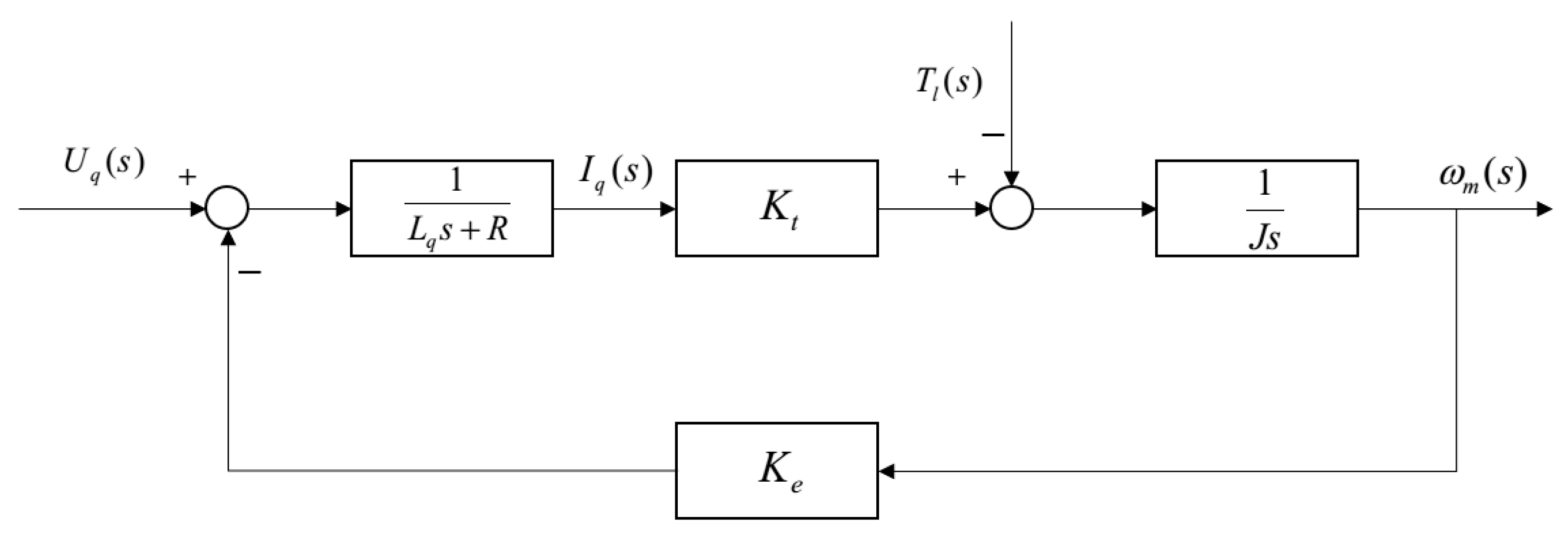
2.1.1. Mathematical Model of PMSM
- 1.
- Stator voltage equationThe stator voltage equation in coordinate system is
- 2.
- Stator flux linkage equationThe stator flux linkage equation in coordinate system is
- 3.
- Electromagnetic torque equationThe electromagnetic torque equation in coordinate system is
- 4.
- Motion equilibrium equationThe equation of motion in coordinate system remains unchanged, which is
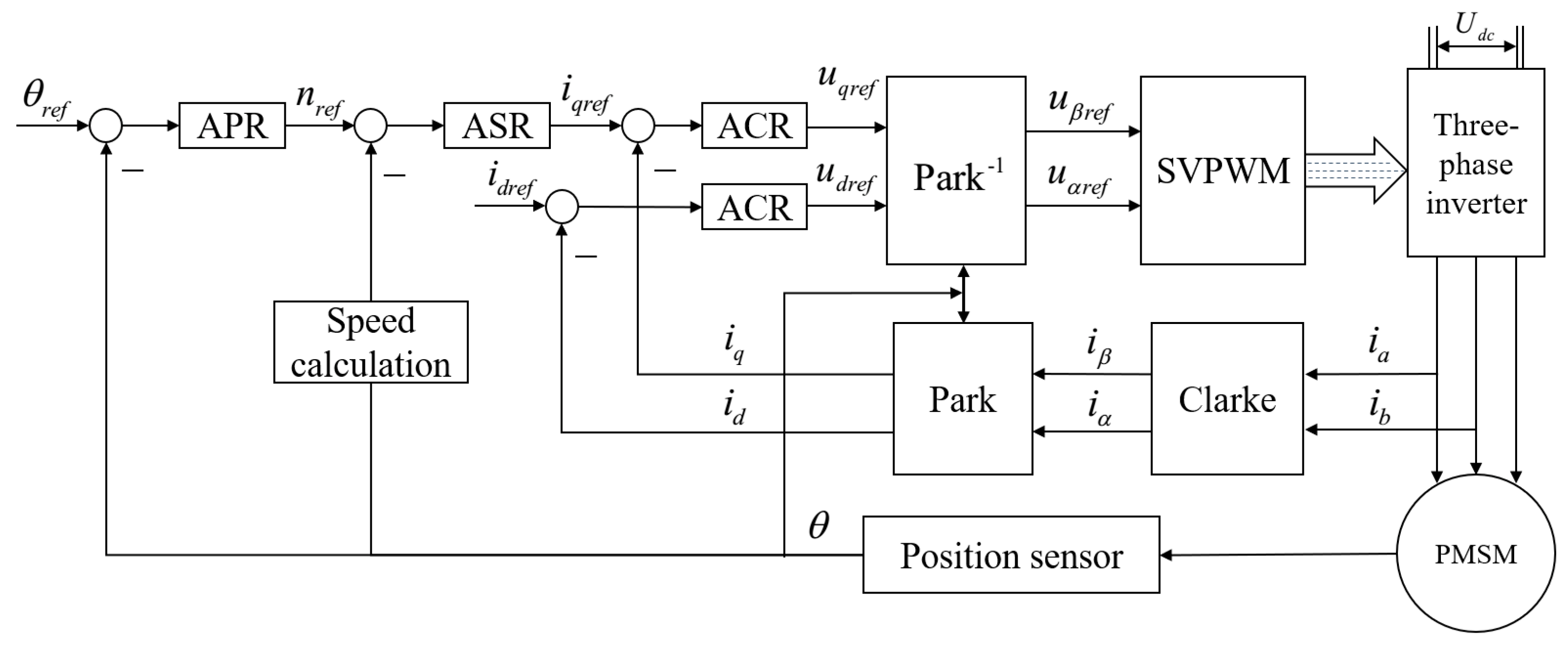
2.1.2. Vector Control Technology
2.1.3. Three Closed-Loop Controller Design
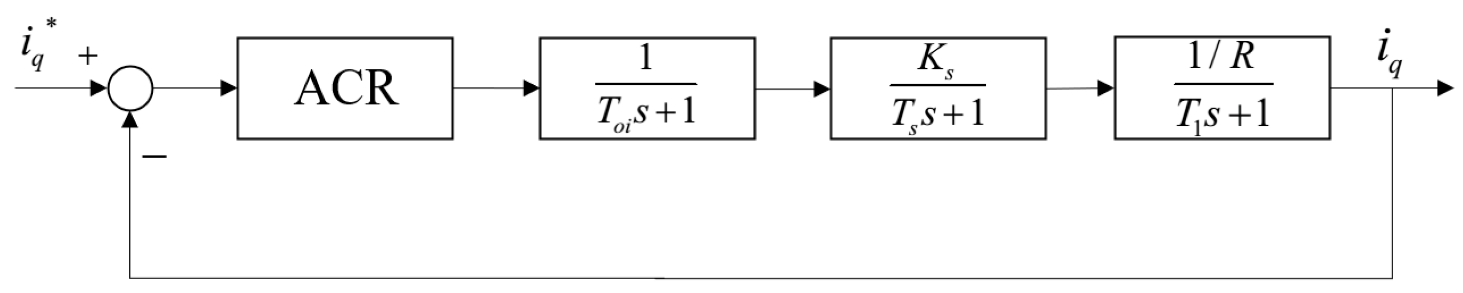
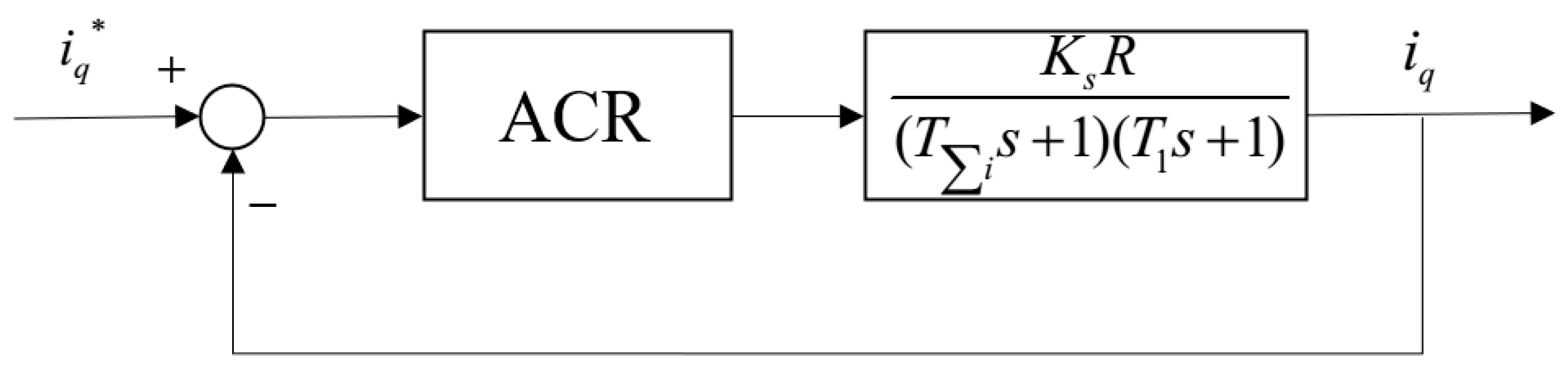
- 1.
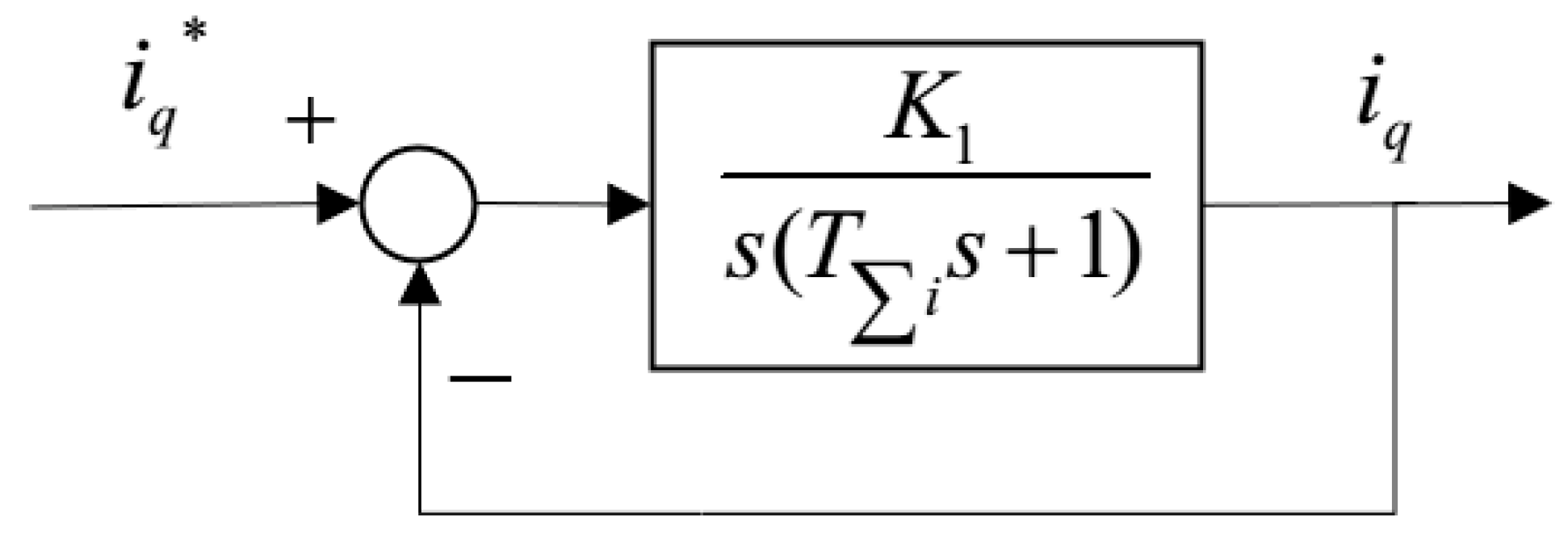
- Current loop design
- 2.
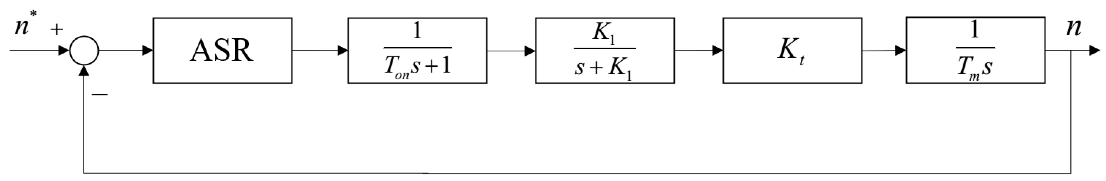
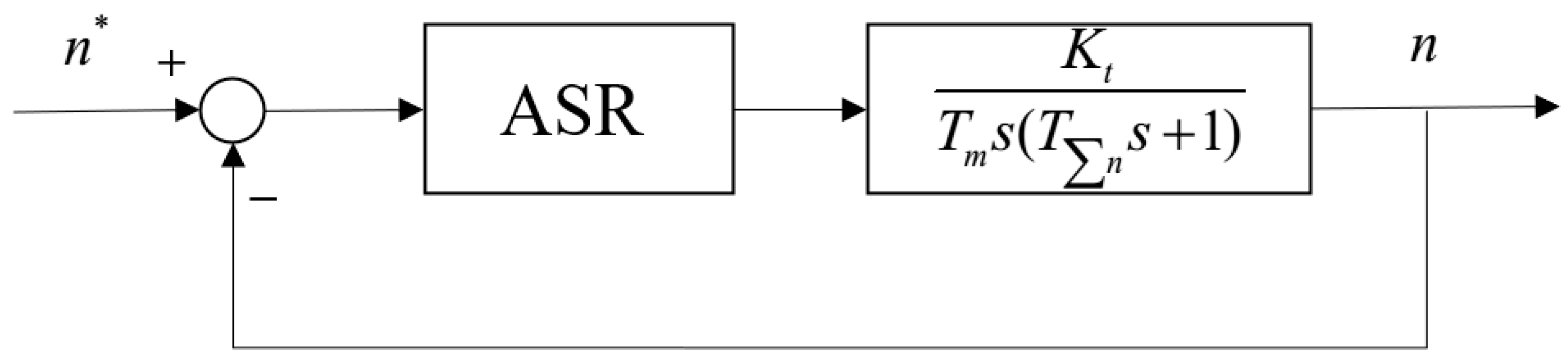
- Speed loop design
- 3.
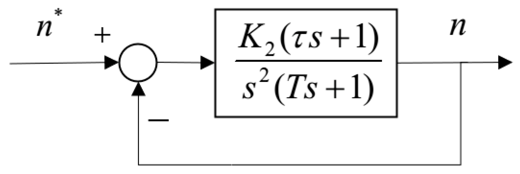
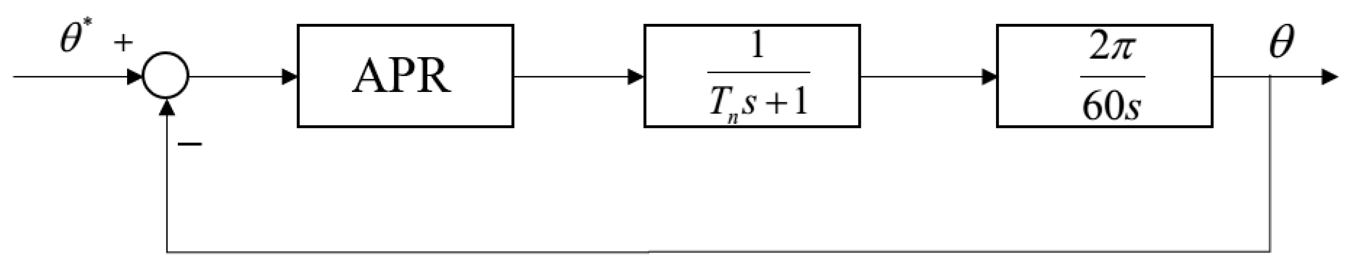
- Position loop design
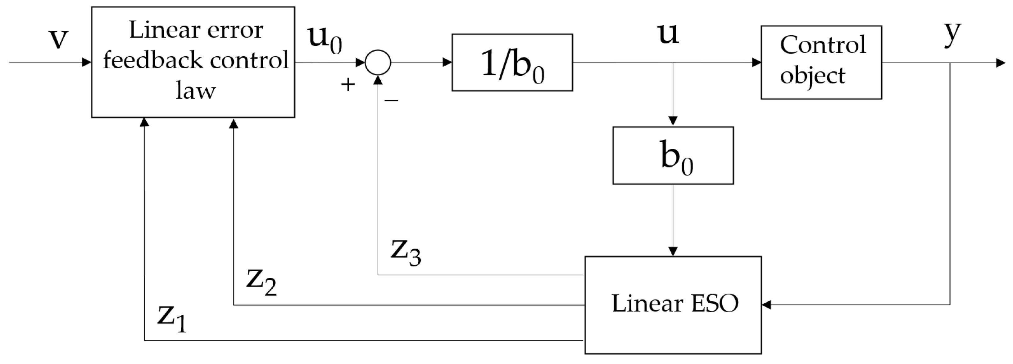
2.2. Linear ADRC
2.2.1. Improved ESO
2.2.2. Linear Error Feedback Control Law
2.3. Design of Linear Active Disturbance Rejection Controller for PMSM
2.3.1. Design of Active Disturbance Rejection Controller for the Speed Loop
2.3.2. Design of the Position Loop ADRC
2.3.3. Stability Analysis of ADRC
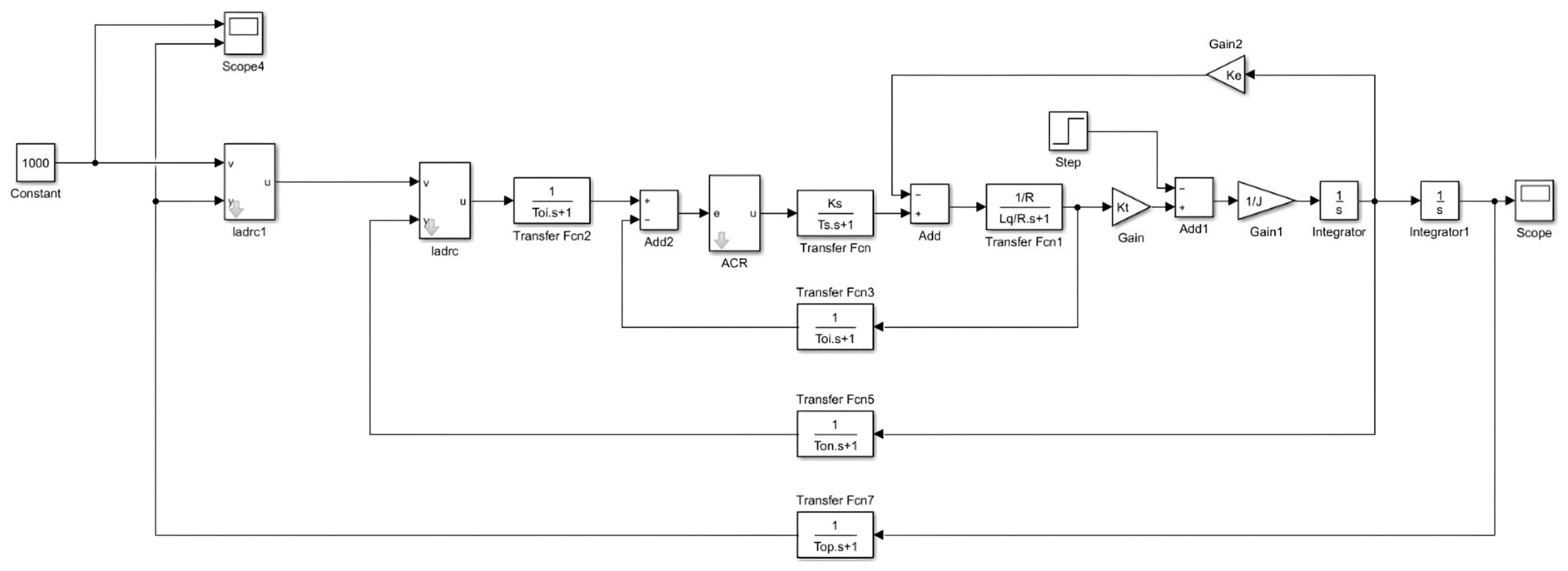
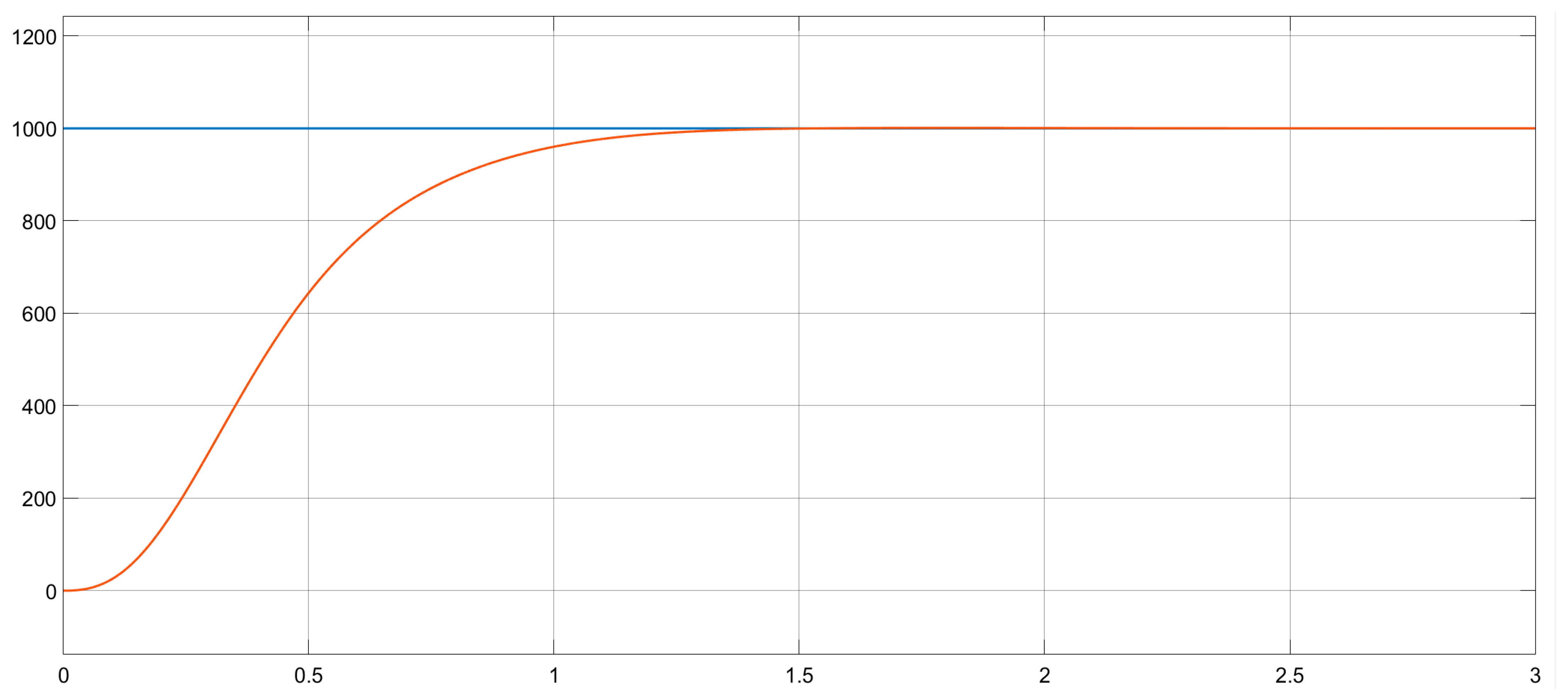
2.4. Simulation of the Linear ADRC System for PMSM
3. Results
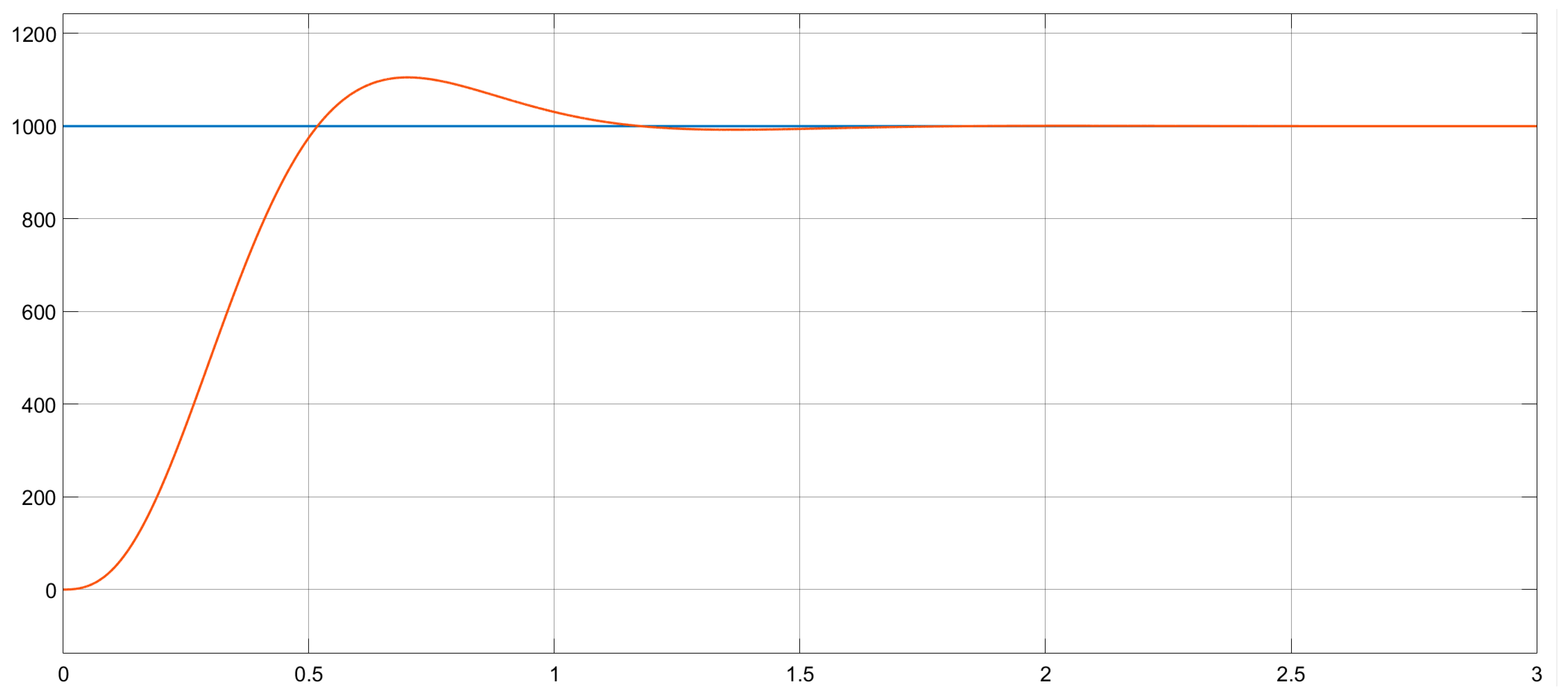
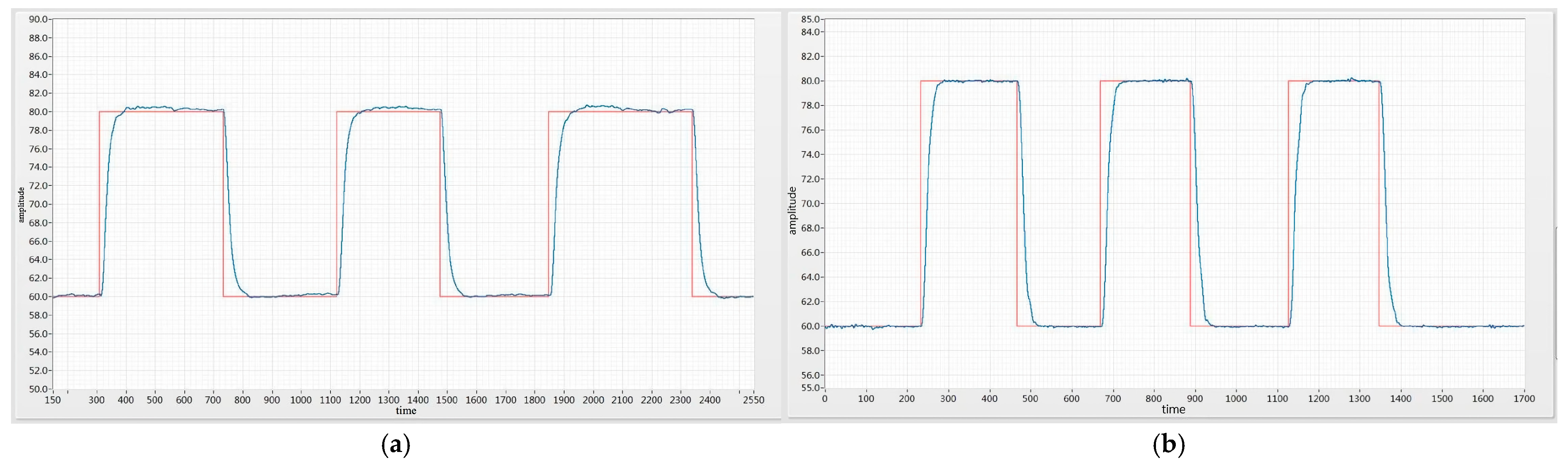
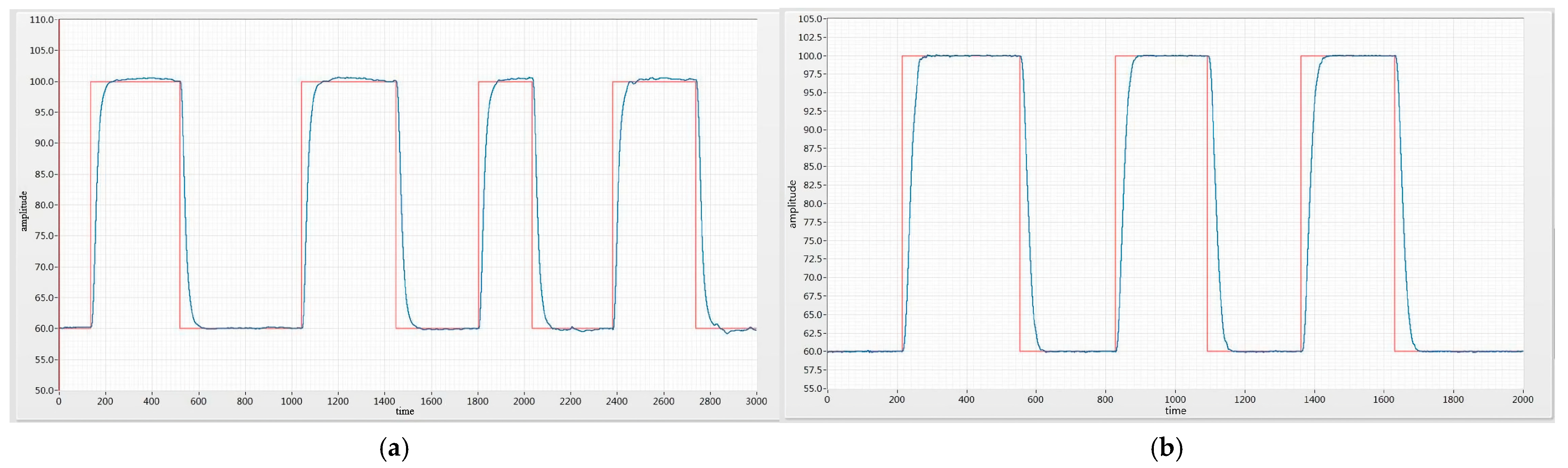
3.1. Load Step Test
3.2. Load Disturbance Test
4. Discussion
- In the aspect of mathematical modeling, the nonlinear factors such as the clearance and friction of the mechanical system are simplified, and the model is not accurate enough, which needs further improvement;
- In terms of the calculation method, the discretization method adopted is the Euler method. The approximate accuracy is not high enough, and it is easy to produce a high-frequency tremor. A better discretization method can be adopted;
- In the system test, the output of the sensor is analog, which is easily affected by noise. The digital sensor can be used to improve the measurement accuracy. The loading mode of the load also needs to be improved.
5. Conclusions
Author Contributions
Funding
Institutional Review Board Statement
Informed Consent Statement
Data Availability Statement
Conflicts of Interest
References
- Wang, F.; Liu, E.; Wang, R.; Zhang, W.; Yang, Y. An approach to improve active disturbance rejection control. Int. J. Control 2020, 93, 1063–1073. [Google Scholar] [CrossRef]
- Fu, C.; Tan, W. Analysis and tuning of reduced-order active disturbance rejection control. J. Frankl. Inst. 2021, 358, 339–362. [Google Scholar] [CrossRef]
- Feng, H.; Guo, B. Active disturbance rejection control: Old and new results. Annu. Rev. Control 2017, 44, 238–248. [Google Scholar] [CrossRef]
- Patelski, R.; Dutkiewicz, P. On the stability of ADRC for manipulators with modelling uncertainties. ISA Trans. 2020, 102, 295–303. [Google Scholar] [CrossRef] [PubMed]
- Fu, C.; Tan, W. Control of unstable processes with time delays via ADRC. ISA Trans. 2017, 71, 530–541. [Google Scholar] [CrossRef] [PubMed]
- Boldea, I.; Tutelea, L.N.; Parsa, L.; Dorrell, D. Automotive Electric Propulsion Systems with Reduced or No Permanent Magnets: An Overview. IEEE Trans. Ind. Electron. 2014, 61, 5696–5711. [Google Scholar] [CrossRef]
- Zhou, C. Research on EMA Digital Servo Control System. Master’s Thesis, Nanjing University of Aeronautics and Astronautics, Nanjing, China, 2013. [Google Scholar]
- Ma, Y. Research and Implementation of Control Strategy for EMA Servo Drive System. Master’s Thesis, Nanjing University of Aeronautics and Astronautics, Nanjing, China, 2018. [Google Scholar]
- Ruiz-Carcel, C.; Starr, A. Data-Based Detection and Diagnosis of Faults in Linear Actuators. IEEE Trans. Instrum. Meas. 2018, 67, 2035–2047. [Google Scholar] [CrossRef]
- Sun, B.; Gao, Z. A DSP-based active disturbance rejection control design for a 1-kW H-bridge DC-DC power converter. IEEE Trans. Ind. Electron. 2005, 52, 1271–1277. [Google Scholar] [CrossRef]
- Gao, Z. Active Disturbance Rejection Control: A paradigm shift in feedback control system design. In Proceedings of the American Control Conference, Minneapolis, MN, USA, 14–16 June 2006. [Google Scholar]
- Qing, Z.; Gao, Z. On Practical Applications of Active Disturbance Rejection Control. In Proceedings of the Chinese Control conference, Beijing, China, 29–31 July 2010. [Google Scholar]
- Zheng, Q.; Gao, L.; Gao, Z. On Validation of Extended State Observer through Analysis and Experimentation. J. Dyn. Syst. Meas. Control 2012, 134, 024505. [Google Scholar] [CrossRef]
- Shi, Z.; Zhang, P.; Lin, J.; Ding, H. Permanent Magnet Synchronous Motor Speed Control Based on Improved Active Disturbance Rejection Control. Actuators 2021, 10, 147. [Google Scholar] [CrossRef]
- Zuo, Y.; Ge, X.; Zheng, Y.; Chen, Y.; Wang, H.; Woldegiorgis, A.T. An Adaptive Active Disturbance Rejection Control Strategy for Speed-Sensorless Induction Motor Drives. IEEE Trans. Transp. Electrif. 2022, 8, 3336–3348. [Google Scholar] [CrossRef]
- Alonge, F.; Cirrincione, M.; D’Ippolito, F.; Pucci, M.; Sferlazza, A. Active disturbance rejection control of linear induction motor. IEEE Trans. Ind. Appl. 2017, 53, 4460–4471. [Google Scholar] [CrossRef]
- Sira-Ramírez, H.; Linares-Flores, J.; García-Rodríguez, C.; Contreras-Ordaz, M.A. On the control of the permanent magnet synchronous motor: An active disturbance rejection control approach. IEEE Trans. Control. Syst. Technol. 2014, 22, 2056–2063. [Google Scholar] [CrossRef]
- Alonge, F.; Cirrincione, M.; D’Ippolito, F.; Pucci, M.; Sferlazza, A. Robust active disturbance rejection control of induction motor systems based on additional sliding-mode component. IEEE Trans. Ind. Electron. 2017, 64, 5608–5621. [Google Scholar] [CrossRef]
- Kato, T.; Xu, Y.; Tanaka, T.; Shimazaki, K. Force control for ultraprecision hybrid electric-pneumatic vertical-positioning device. Inter-Natl. J. Hydromechatronics 2021, 4, 185–201. [Google Scholar] [CrossRef]
- Togawa, T.; Tachibana, T.; Tanaka, Y.; Peng, J. Hydro-disk-type of electrorheological brakes for small mobile robots. Int. J. Hydromechatronics 2021, 4, 99–115. [Google Scholar] [CrossRef]
- Yoo, D.; Yau, S.T.; Gao, Z. Optimal fast tracking observer bandwidth of the linear extended state observer. Int. J. Control 2007, 80, 102–111. [Google Scholar] [CrossRef]
- Yoo, D.; Yau, S.T.; Gao, Z. On Convergence of the Linear Extended State Observer. In Proceedings of the 2006 IEEE Conference on Computer Aided Control System Design, 2006 IEEE International Conference on Control Applications, 2006 IEEE International Symposium on Intelligent Control, Munich, Germany, 4–6 October 2006. [Google Scholar]
- Colgren, R.; Frye, M. The design and integration of electromechanical actuators within the U-2S aircraft. In Proceedings of the Guidance, Navigation, and Control Conference and Exhibit, Beijing, China, 22 August 2012. [Google Scholar]
- Chen, G.; Zeng, M.; Wei, L. Overview of sensorless permanent magnet synchronous motor vector control system. Weite Mot. 2011, 39, 64–67. [Google Scholar]
- Zhu, B. Introduction to Active Disturbance Rejection Control; Beijing University of Aeronautics and Astronautics Press: Beijing, China, 2017. [Google Scholar]


Disclaimer/Publisher’s Note: The statements, opinions and data contained in all publications are solely those of the individual author(s) and contributor(s) and not of MDPI and/or the editor(s). MDPI and/or the editor(s) disclaim responsibility for any injury to people or property resulting from any ideas, methods, instructions or products referred to in the content. |
© 2023 by the authors. Licensee MDPI, Basel, Switzerland. This article is an open access article distributed under the terms and conditions of the Creative Commons Attribution (CC BY) license (https://creativecommons.org/licenses/by/4.0/).
Share and Cite
Fang, Q.; Zhou, Y.; Ma, S.; Zhang, C.; Wang, Y.; Huangfu, H. Electromechanical Actuator Servo Control Technology Based on Active Disturbance Rejection Control. Electronics 2023, 12, 1934. https://doi.org/10.3390/electronics12081934
Fang Q, Zhou Y, Ma S, Zhang C, Wang Y, Huangfu H. Electromechanical Actuator Servo Control Technology Based on Active Disturbance Rejection Control. Electronics. 2023; 12(8):1934. https://doi.org/10.3390/electronics12081934
Chicago/Turabian StyleFang, Qian, Yong Zhou, Shangjun Ma, Chao Zhang, Ye Wang, and Haibin Huangfu. 2023. "Electromechanical Actuator Servo Control Technology Based on Active Disturbance Rejection Control" Electronics 12, no. 8: 1934. https://doi.org/10.3390/electronics12081934