
Obstacle Avoidance Strategy for Mobile Robot Based on Monocular Camera


1
Department of Mechatronics, School of Mechanical Engineering, Hanoi University of Science and Technology, Hanoi 10000, Vietnam
2
Shibaura Institute of Technology, Saitama 337-8570, Japan
*
Author to whom correspondence should be addressed.
Electronics 2023, 12(8), 1932; https://doi.org/10.3390/electronics12081932
Submission received: 4 March 2023
/
Revised: 14 April 2023
/
Accepted: 18 April 2023
/
Published: 19 April 2023
(This article belongs to the Special Issue Machine Learning (ML) and Software Engineering)
Abstract
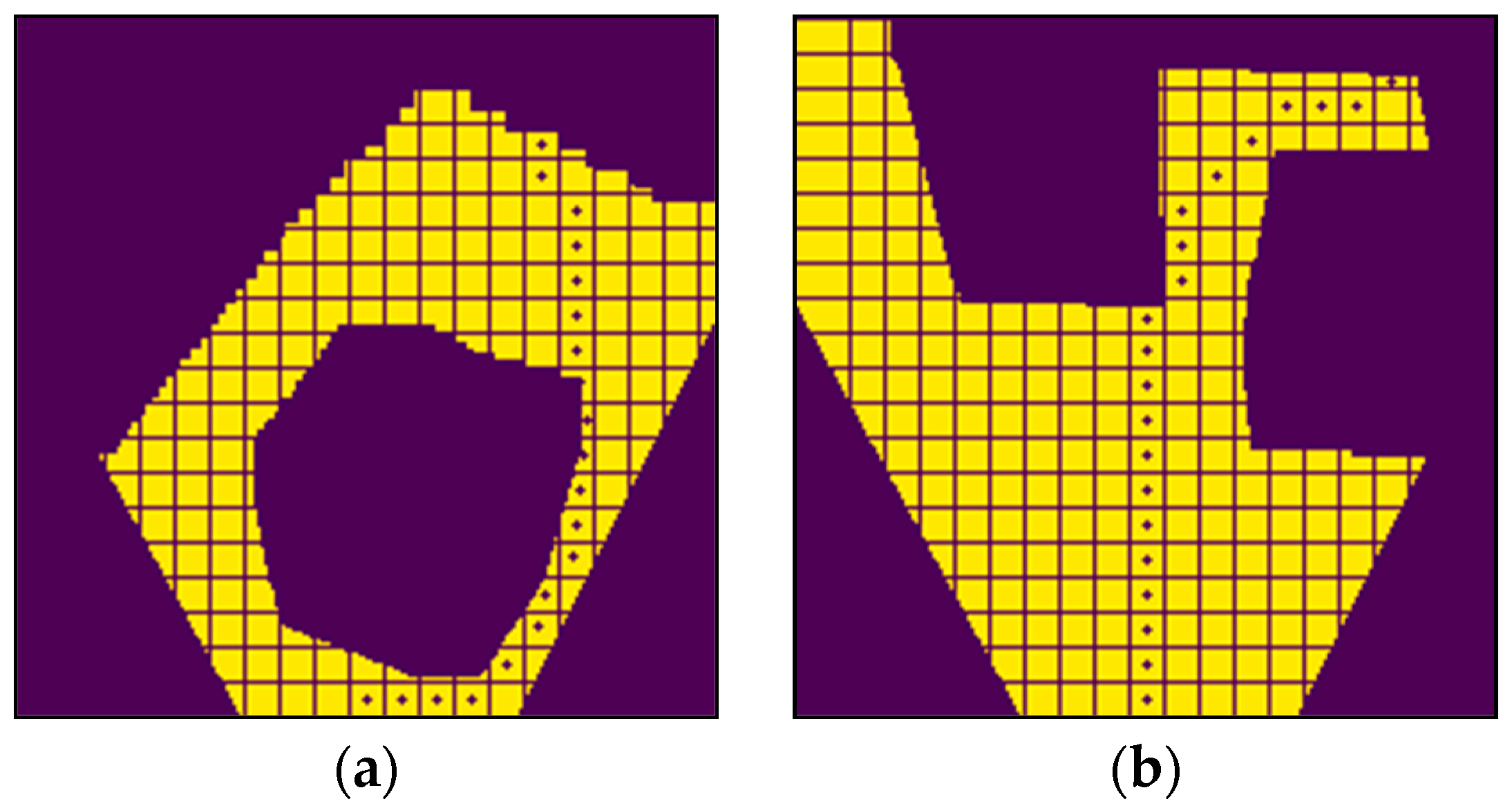
:This research paper proposes a real-time obstacle avoidance strategy for mobile robots with a monocular camera. The approach uses a binary semantic segmentation FCN-VGG-16 to extract features from images captured by the monocular camera and estimate the position and distance of obstacles in the robot’s environment. Segmented images are used to create the frontal view of a mobile robot. Then, the optimized path planning based on the enhanced A* algorithm with a set of weighted factors, such as collision, path, and smooth cost improves the performance of a mobile robot’s path. In addition, a collision-free and smooth obstacle avoidance strategy will be devised by optimizing the cost functions. Lastly, the results of our evaluation show that the approach successfully detects and avoids static and dynamic obstacles in real time with high accuracy, efficiency, and smooth steering with low angle changes. Our approach offers a potential solution for obstacle avoidance in both global and local path planning, addressing the challenges of complex environments while minimizing the need for expensive and complicated sensor systems.
1. Introduction
The capacity to avoid obstacles is the primary goal of autonomous navigation, which demands precision and efficiency. Thus, autonomous mobile robots (AMRs) must be able to identify environmental barriers and design avoidance maneuvers. Sonars [1], infrared (IR) sensors [2], laser scanners [3], and cameras [4] are only a few examples of the many technologies developed to address the challenge of mobile robot navigation. Sonar devices in various mounting configurations were utilized for many years for obstacle detection due to their great low cost, although suffering from large inaccuracy due to reflection [5]. Due to the repeated teaching process, the processing time is extremely lengthy. Because the path finding method can be developed based on the connection between the destination and target point, the navigation process is not ideal. Laser scanners were shown to be trustworthy and accurate. Nevertheless, they become problematic in uncharted territory [6]. Cameras give rich scene information despite their small footprint, inexpensive cost, and high computing power requirements [6]. The proposed method removed those restrictions because low-cost monocular cameras of sufficient precision are now widely available. Because of their perceptual abilities, AMRs recently saw a rise in popularity as a sensing approach based on vision-based navigation [7]. Recent years saw extensive research into monocular depth estimates using deep learning, and the results are encouraging [8]. Hence, real-time image segmentation-based navigation was effectively completed [9].
In many vision-based applications, such as scene understanding, robotic perception, and picture reduction [10,11,12,13,14], semantic segmentation using deep learning (DL) is a fundamental problem. Minae et al. [10] examined DL-based segmentation models that showed remarkable performance in visual image segmentation tests to address lack of regular datasets for evaluating object segmentation. Then, using a shared dataset, Li et al. [11] selected the most appropriate strategy from various structures of semantic segmentation. The ISPRS Vaihingen 2D semantic labeling contest was enhanced in [12] to address this issue. With limited samples, the semi-supervised self-learning method maintained semantic segmentation accuracy. Image semantic segmentation with hierarchical feature fusion (ISHF) was presented by Yang et al. [13] to ensure the accuracy of picture segmentation in deep neural networks. Despite ensuring the accuracy of segmentation, there were issues with improving segmentation speed. Fusic et al. [14] proposed a vision sensor-based DL algorithm to classify obstacles and terrain from the evaluation of the obtained image files. However, the navigation based on scene terrain classification was not ultimately demonstrated. Moreover, the vision-based navigation was enhanced by combining it with the sensor system. Gharajeh et al. [15] proposed mobile robot path planning based on the ANFIS technique. However, to save memory resources and fast processing time in the perception, the authors applied binary semantic segmentation, such as moving and restricted regions. The segmentation framework is now more efficient and lightweight without sacrificing quality. There is now both a global and a local path to the path planning process. The performance of AMRs’ motion depends on environmental perception [15,16,17,18,19,20,21,22,23].
Global path planning is only applicable in well-known environments when utilizing well-known techniques, such as the Dijkstra algorithm [16], the A* algorithm [17], and the rapidly exploring random tree (RRT) search method [18]. In close quarters, we employ local path planning strategies, such as the dynamic window approach (DWA) [19], game-theory-based path planning [20], and the ant colony method [21]. Shaher et al. [16] presented a simple, optimal Dijkstra algorithm-based technique for global path planning. Nevertheless, the technique simply restricted nodes with less random access memory (RAM). As a result, the search was essentially inefficient and slow. Eshtehardian et al. [18] developed a rapid RRT* search algorithm combining with B-spline for a smooth trajectory. Although the standard rapid random tree search algorithm entirely handled MOOPs such as smoothness, shortest path, and collision avoidance, the ideal technique required more memory and processing time. Although it converged slowly, [21]’s ant colony algorithm was trustworthy. Based on the Dijkstra algorithm [16], the A* algorithm was a heuristic search tool [17]. In a large and complicated environment, the A* algorithm alone could not be used for path planning. Yonggang et al. [23] suggested an efficient A* approach combining with the three-time Bezier curve to address the concerns of diverse turning points and steering angles. Enhanced A* algorithms are widely utilized for both global and local path planning due to their fast calculation speeds, path optimization, and other advantages.
The authors successfully design multi-scale fully convolutional network-based semantic segmentation for mobile robot navigation using a low resource system. Then, we completely utilize perspective correction on the segmented image to generate the AMR’s frontal view of the moving environment, which detects the real-time moving area. In addition, the optimized path planning algorithm is implemented based on the monocular camera. Data processing, thus, calls for adequate performance and speed rate despite constrained means. All three costs work together to guarantee the shortest path, the minimum distance to obstacles, and a smooth trajectory. The structure of the paper consists of the following sections: After the introduction, the binary semantic segmentation based on VGG-16 provides two foundational stages of segmentation network architecture and training process. Next, navigation strategy based on ground plane segmentation describes the foundational stages for constructing an optimal obstacle avoidance navigation strategy. In addition, the approach is strengthened and effectively validated in Experimental Results. The conclusion finishes with a summary and a development of future projects.
2. Binary Semantic Segmentation FCN-VGG-16
The suggested binary semantic segmentation based on VGG-16 has two primary components: network architecture and network training. The following two sections elaborate on these two sections (Section 2.1 and Section 2.2).
2.1. Network Architecture
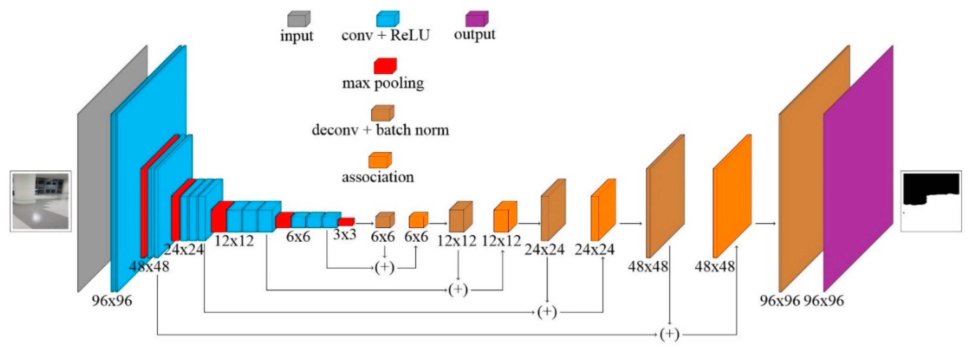
The authors develop a network based on the FCN [24,25,26,27] to accomplish instant pixel-wise labeling while maintaining a decent segmentation outcome. VGG [25] is chosen over AlexNet [26] because of its popularity and more accurate predictions. In contrast to prior work by Shelhamer et al. [27], our binary semantic segmentation based on VGG-16 [7] employs deconvolutional layers at a total of four scales. The authors use different scales to refine their predictions significantly. According to Yang et al. [28], this architecture starts with a low-resolution, rough output prediction and refines it by fusing with prior layers to give both local and global reasoning. VGG-16 is introduced as a convolutional and max pooling layer-based encoder block in this case, as shown in Figure 1. All of the hidden layers rely on linear rectifiers as their activation source. The completed VGG-16 layers are removed from the network. The authors use multiscale fusions to merge features taken from various layers to build the decoder block. The network input is a 96 × 96 × 3 RGB image, and the first scaler’s output is 1/32 of the input image’s size. The network will then be upsampled to the necessary image size of 96 × 96 × 64 by a classifier transforming the shape to 96 × 96 × C. The number of classes C is used for intending to segment semantically. The number of classes C is set to two because we only wish to mark pixels that belong to the ground and those that do not. Ceilings, doorways, and pillars were not labeled because they are unimportant for the majority of robot navigation purposes, although their labels might be simply added if necessary.
2.2. Network Training
The experiments were executed on a server outfitted with specific software and an operating system. To be precise, the server was equipped with Python 3.11.0 and the TensorFlow 1.4 framework and ran on 64-bit Windows 10 Home English. The server was powered by an Intel(R) Core (TM) I7-8750 h processor, operating at either 2.20 GHz or 2.21 GHz.
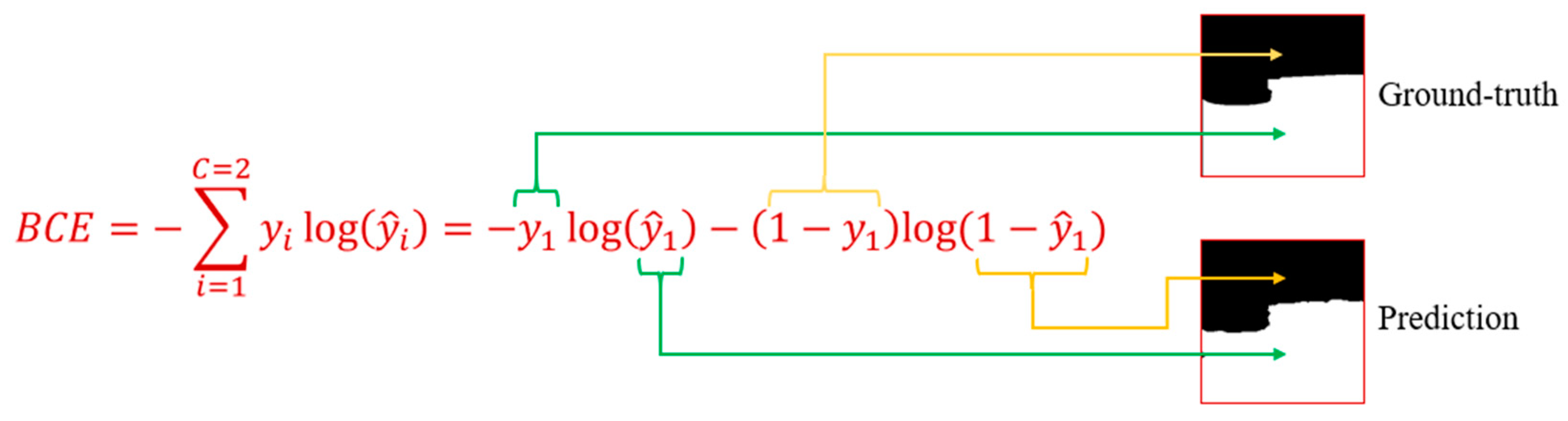
where is the class softmax probability; is the prediction’s ground truth. The dataset is similar to the source of data in [7]. The corridor environment plays an essential role in AMRs motion, which often motivates the authors to gather corridor-specific training datasets. The forecast of FCN-VGG-16 is depicted in detail in Figure 2 based on Equation (1).
Because of the difficulty of categorizing data, the authors settle on cross-entropy loss. For classification models where the output is a probability value between 0 and 1, a standard performance measure is cross-entropy loss, often known as log loss. While cross-entropy and log loss have subtle differences depending on the setting, they are equal for assessing error rates between 0 and 1 in machine learning. When C = 2, it is referred to as binary cross-entropy or BCE in Equation (1).
Network parameters are optimized for binary cross-entropy via one of the SGD variants’ parameter learning strategies. In contrast to the suggestion made by Yang et al. [28], our network’s capabilities were increased through data augmentation, in which the original versions of the training images are used. The training process is sped significantly thanks to the extensive use of transfer learning. The authors use trained VGG models to set the network parameters. The only challenging part is picking the right training environment. After training and validating many different network versions, as shown in [7], the authors settled on the following parameters: the momentum is 0.9, and the learning rate is 0.001; the training procedure is tuned for 300 epochs, and the learning rate is decayed by 10 for every 80 epochs.
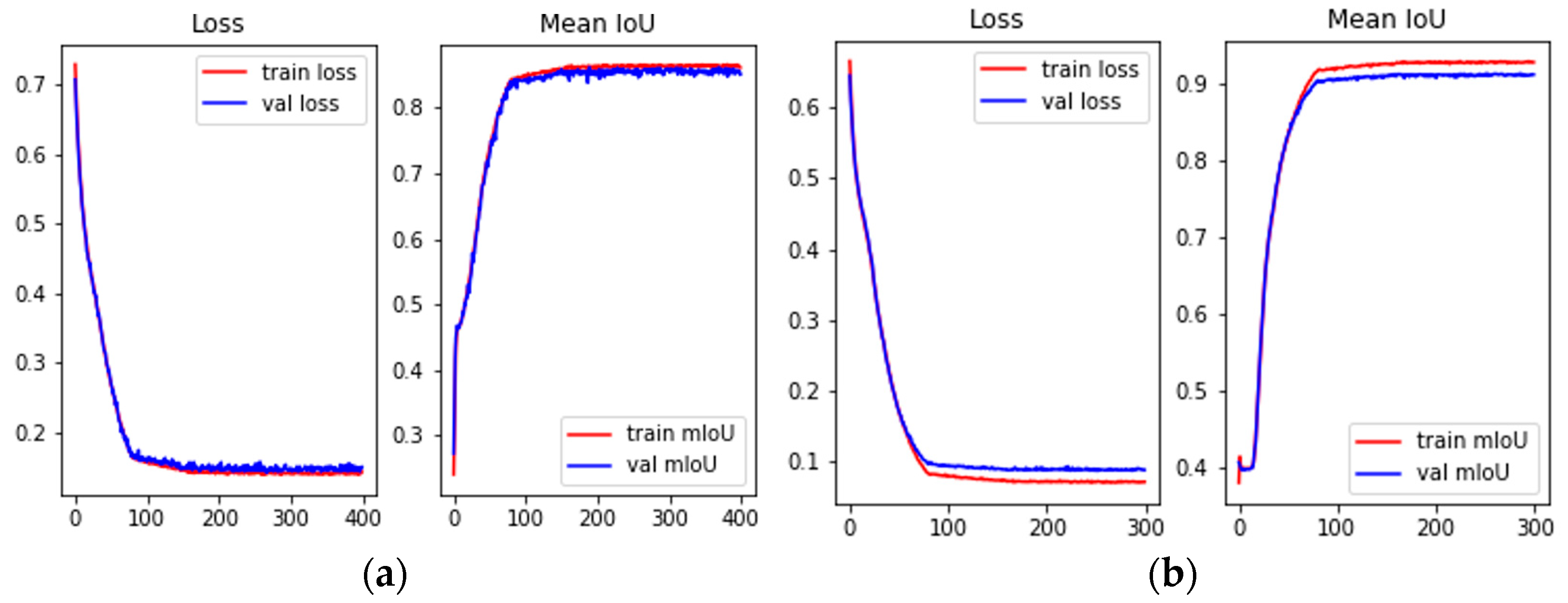
When using a multi-scale FCN for binary semantic segmentation, the authors get two classes, accessible and inaccessible areas. Hence, with limited resources, enough performance and speed rate in data processing is necessary. The image size of 96 × 96 was exclusively chosen. Training times are cut thanks to the widespread use of transfer learning drastically. The authors use pre-trained VGG models to set up the network, with the most complicated part being the choice of training parameters through training and testing numerous network versions in Figure 3. Figure 3a represents the validation mIoU as the noise impacting the quality of the training process and how it can be reduced to speed up the training process. As a result, the accuracy of the forecast will drop. The authors take measures to avoid overfitting by augmenting their data. The method makes it easier to fine-tune the forecast shown in Figure 3b. Additionally, practically eliminating noise will considerably improve the quality of the prediction. The segmentation noise filtering method is finalized using the probabilistic models described in [28].
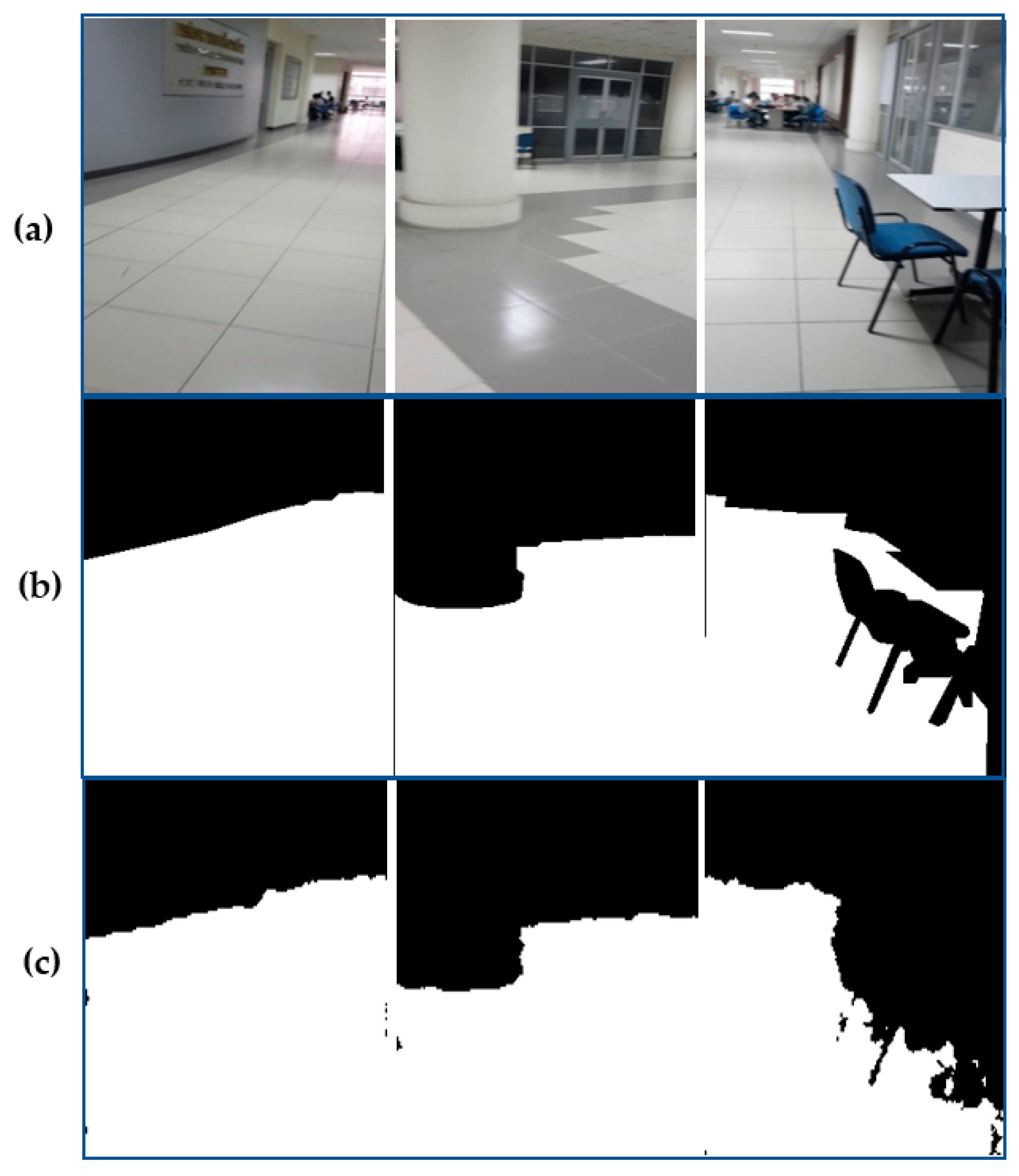
In these difficult scenarios, our network is able to accurately anticipate the ground border, demonstrating its tolerance to different corridor types. The segmentation experiment outcomes in the Ta Quang Buu library setting are depicted in Figure 4.
Finally, the optimal autonomous mobile robot path planning in the next section is guaranteed by the binary semantic segmentation VGG-16’s output results.
3. Navigation Strategy Based on Ground Plane Segmentation
Our proposed approach constructs the fraction map based on the current observation, using the result of the binary semantic segmentation process in which the available area for movement of the arbitrary view will be labeled. Because inaccurate segmentation affects obstacle avoidance results. So, the segmentation model output will be continuously put into the probabilistic model using conditional random fields to filter the noise and uncertainty [29] completely. Furthermore, the quality of the architecture of the segmentation model also affects the results [30]. The navigation strategy of mobile robots includes three sections as follows: In Section 3.1, a perspective correction method is used to alter the ground region extracted from the semantic segmentation result. Section 3.2 provides a sequence of coordinates for precise navigation from the current place to the designated destination, based on a bird’s-eye perspective. Finally, Section 3.3 concludes by discussing the ideal trajectory strategy for mobile robots. These three sections are further upon in the sections that follow.
3.1. Perspective Correction
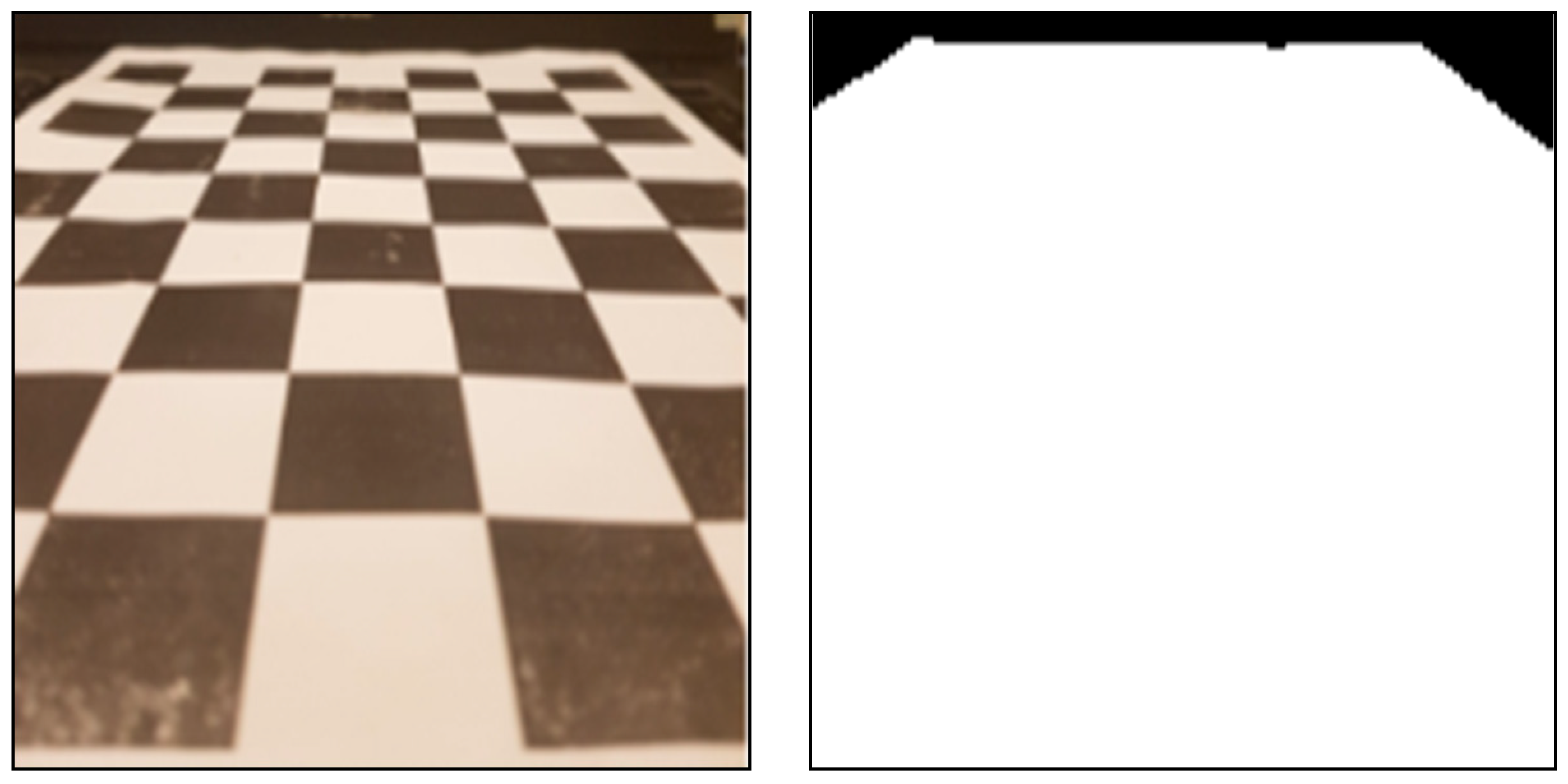
Figure 5 shows the images obtained after the binary semantic segmentation procedure, labeling functional movement (white) and prohibited regions (black). Measurements of the distance to the obstruction were complicated by the strong distortion caused by the perspective of the taken images.
The authors require coordination to be proportional to the actual ground in order to plan the trajectory. To get a rough idea of the connection between world coordinates and image coordinates, we can use a basic matrix multiplication based on the pinhole model and a mathematical camera description. The transformation that maps a point from the world coordinate system to the image coordinate system can be expressed as follows, where p and P denote the image point and the world point, respectively:
where presents the matrix of intrinsic parameters, is the matrix of extrinsic parameters. The intrinsic and extrinsic parameters are internal to the camera; however, the latter can change depending on the camera’s position in the world frame.
The intrinsic and rotational constituents of the extrinsic parameters remain constant, owing to the camera’s configuration mounted on the bird’s eye view of the mobile robot. These parameters are presumed to remain invariant during movement, rendering the approximations calculable only once. Utilizing the correspondence of four points in [31], the front view of the ground plane can be constructed through a transformation matrix. Consequently, our resulting image solely captures the ground plane and the available and unavailable regions. The projective transformation, founded upon the four points, can be described as follows:
Let (x, y) and (x′, y′) be inhomogeneous. Coordinates of a pair of matching points x and x′ are in the world and image plane, and the given n point correspondences satisfy . Then, the transformation H is described such as follows:
with each point correspondence satisfies two constraints:
Hence, H is determined uniquely. Hence, from any four points on the scene plane in Figure 6a, we will obtain four points of arbitrary view in Figure 6b. Finally, transformation H will build any four points of an arbitrary view of a real-time moving environment to any other four points in the frontal view.
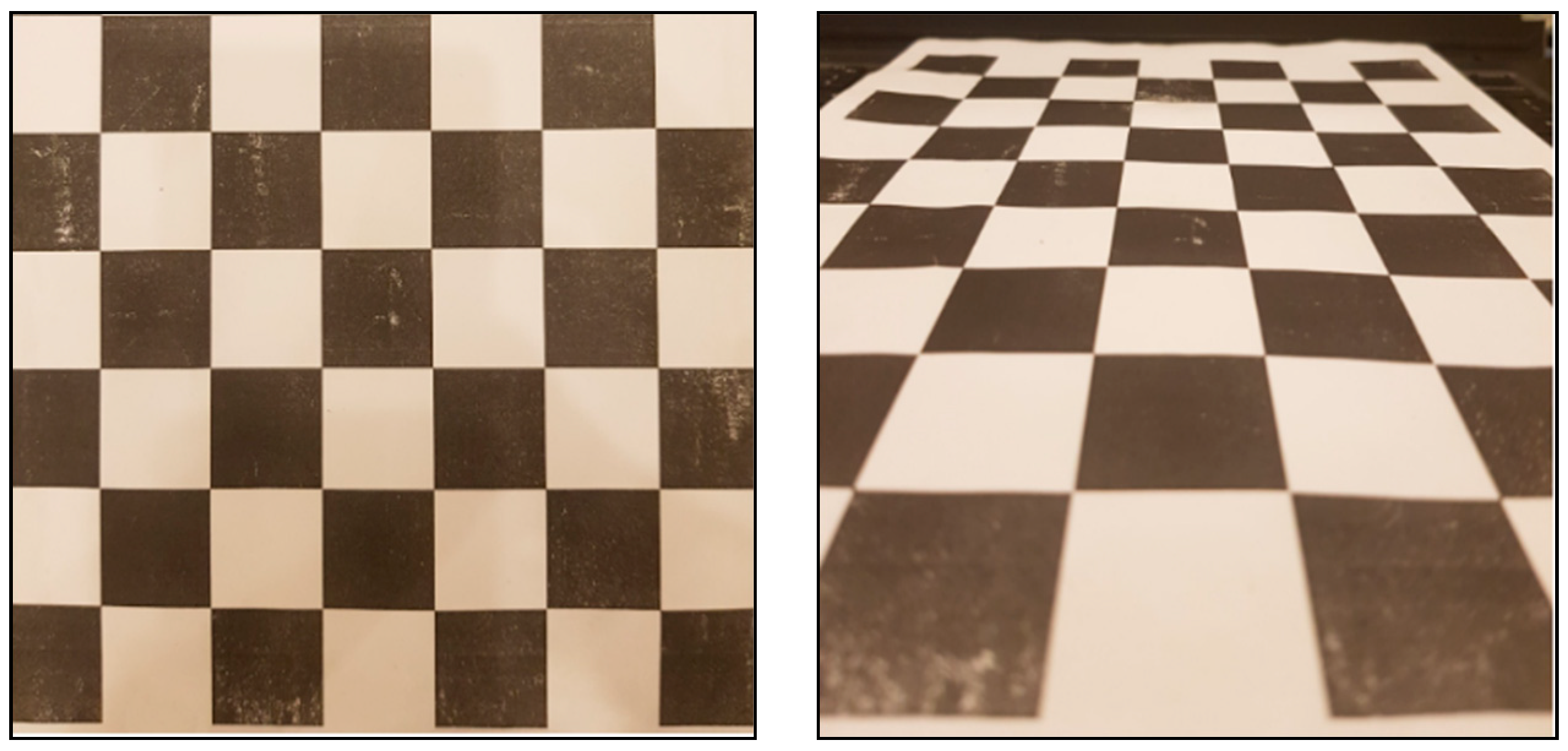
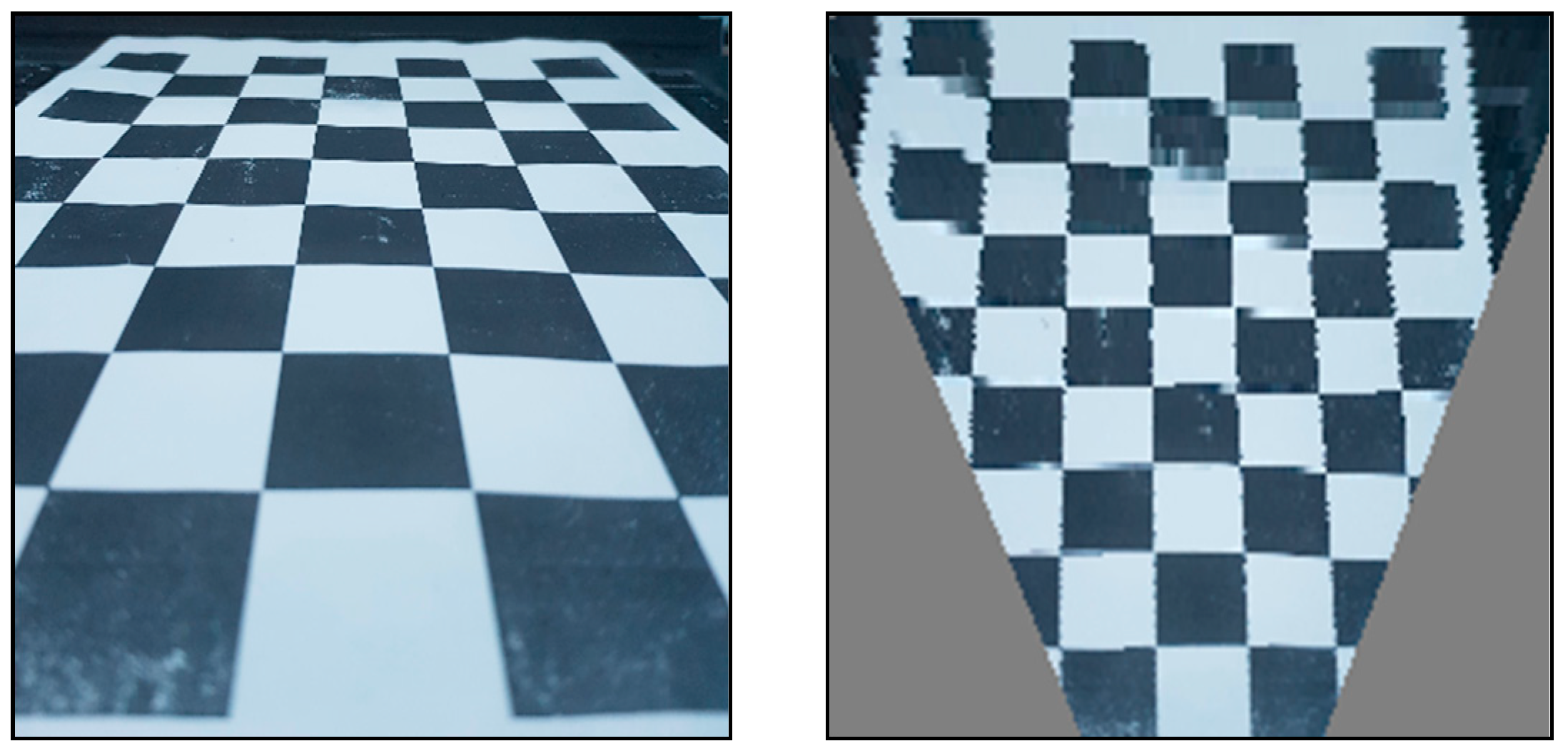
The authors perform the perspective correction of the frontal views by using the checkerboard in Figure 7.
Using the above transformation, the authors can construct the frontal view for a real-time motion to define the available area. Figure 8 shows the segmentation model’s output from frontal view images.
Based on the information perception of the monocular camera bird’s view in Figure 9, mobile robot path planning will be designed entirely.
3.2. Path Planning
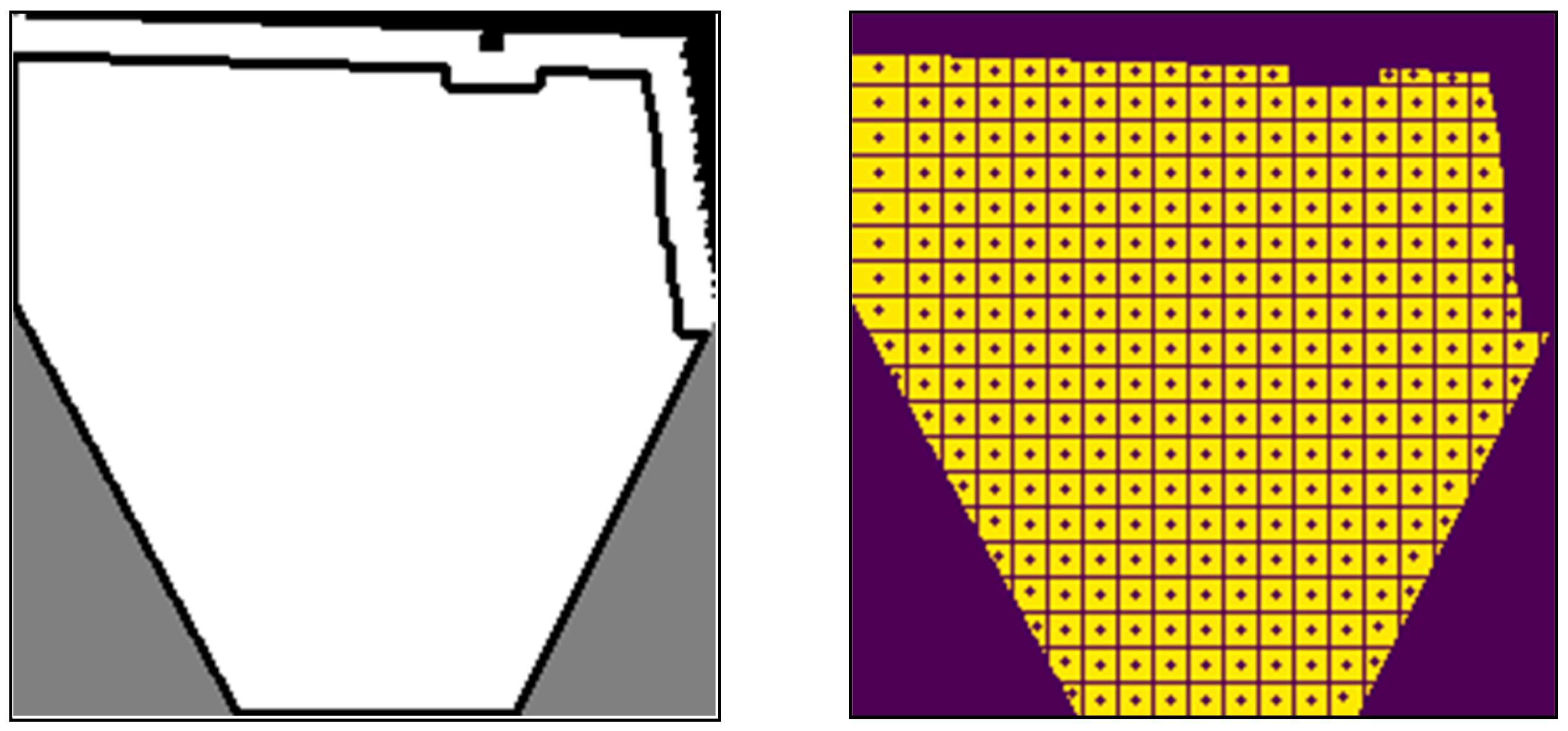
Based on the generated frontal plane, the authors will construct a moving path using a traditional A* algorithm [17]. Firstly, the authors create a collision-free area by scalding up the unavailable place. After that, the image will be divided into grid cells. The current position is determined at the bottom center of the picture. The authors calculate the centers of each cell and use them for the path planning process in Figure 10.
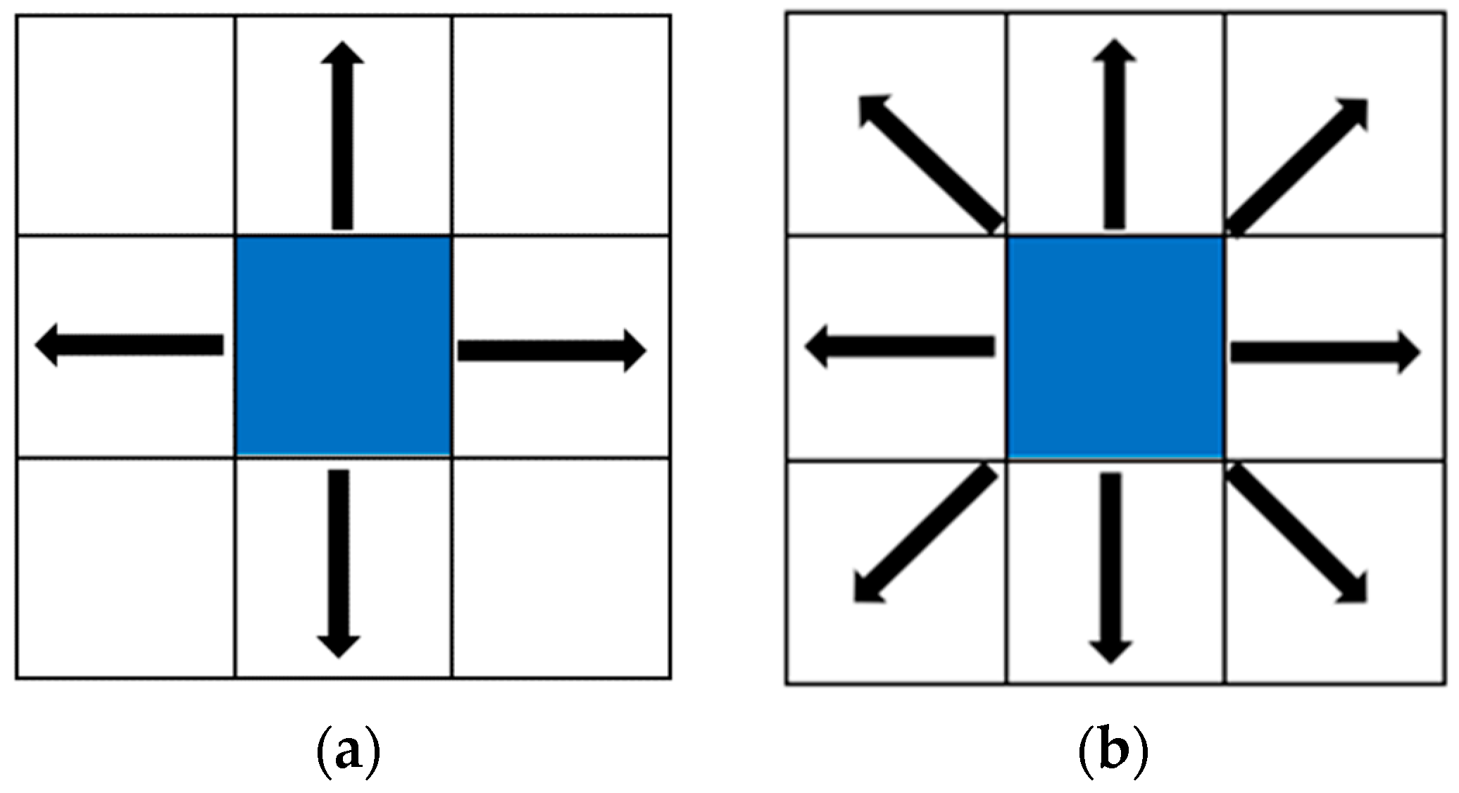
In each mobile robot position, we have five functional movements: left, up—left, straight, up—right, and right. A fundamental aspect of the A* algorithm is its utilization of a heuristic function to estimate the cost to the objective. The heuristic function is a distance-based mathematical estimation of the cost to the target from a given point. By utilizing a heuristic function, the A* algorithm can prioritize points that are likely to be closer to the target, enabling it to identify the shortest path more quickly in Equation (5).
where m represents the current point, f(m) represents the cost evaluation function, h(m) represents the predicted cost from m to G, and g(m) represents the actual cost from m to the next point. The typical heuristic function for distance is the Manhattan distance, as indicated in Equation (6), or the Euclidean geometric distance, as given in Equation (7).
and
is the position of the goal point, and is the coordinate of any point.
Figure 11a shows that the A* algorithm can only search in four directions for neighborhoods when utilizing the Manhattan distance. Figure 11b presents an alternative use of Euclidean distance to study eight neighborhoods. The search process begins at S and then expands to surrounding points. Then, the generation values following are calculated. The generating values are then evaluated using the heuristic function. Finally, the point with the smallest generation value is selected as the next parent point. The search procedure will be repeated until the target point G is located. In a large-scale map, the conventional A* search will generate an enormous number of path points and consume a significant amount of memory.
The heuristic cost is determined by the distance of the current grid cell’s center to the target grid cell’s center, and the path cost is calculated by the distance between the centers of adjacent grid cells. The algorithm repeats the exploration by picking the cell with the lowest price (sum of path cost and heuristic cost) in the priority queue until the picking cell reaches the target (path is found) or the queue is empty (path is not found). If the path is found, the algorithm will construct the absolute path by following the path cost from the target grid cell.
3.3. Trajectory Optimization
After obtaining the path by the A* algorithm, the authors use K points to describe the trajectories and apply the cost function (movement requirement) for the smoothening process. The cost function is constructed based on the necessity of a low steering angle, and a collision-free and continuous path, which is similar to the objective function described as follows:
where , , and are weights of collision cost, path cost, and smooth cost, respectively. Each cost component has a different effect on the result and can be described as follows:
Collision cost Ccollision prevents collision by penalty points that are in the unavailable area and pushes them to the nearest available area:
where are the path coordinates, are the closest collision-free bounding points relative to coordinates p, and is the minimum distance to the nearest obstacle.
Path cost Cpath ensures the continuity of the sequence of coordinates by penalty points goes far from the planned path:
where are the coordinates, are the closest points in the planned path relative to .
Smooth cost Csmooth reduces the steering angle by penalty the sum of the distance of three consecutive points:
where are three consecutive coordinates.
The authors update the optimization using gradient-based methods [32]. In Equation (8), smooth cost Csmooth introduces the risk of inaccuracy. The smooth cost function always decreased the angle between three adjacent coordinates. Thus, the authors apply a weight to the smooth cost based on whether the coordinates fall inside the accessible or unavailable area. When coordinates enter the available area, the update can typically continue. Otherwise, the magnitude of the update will be diminished by the added weight. The influence of the smooth cost remains, but it is less significant than the effect of the collision cost, which will return the coordinates to the available area.
4. Experimental Results
4.1. Proposed Obstacle Avoidance Strategy
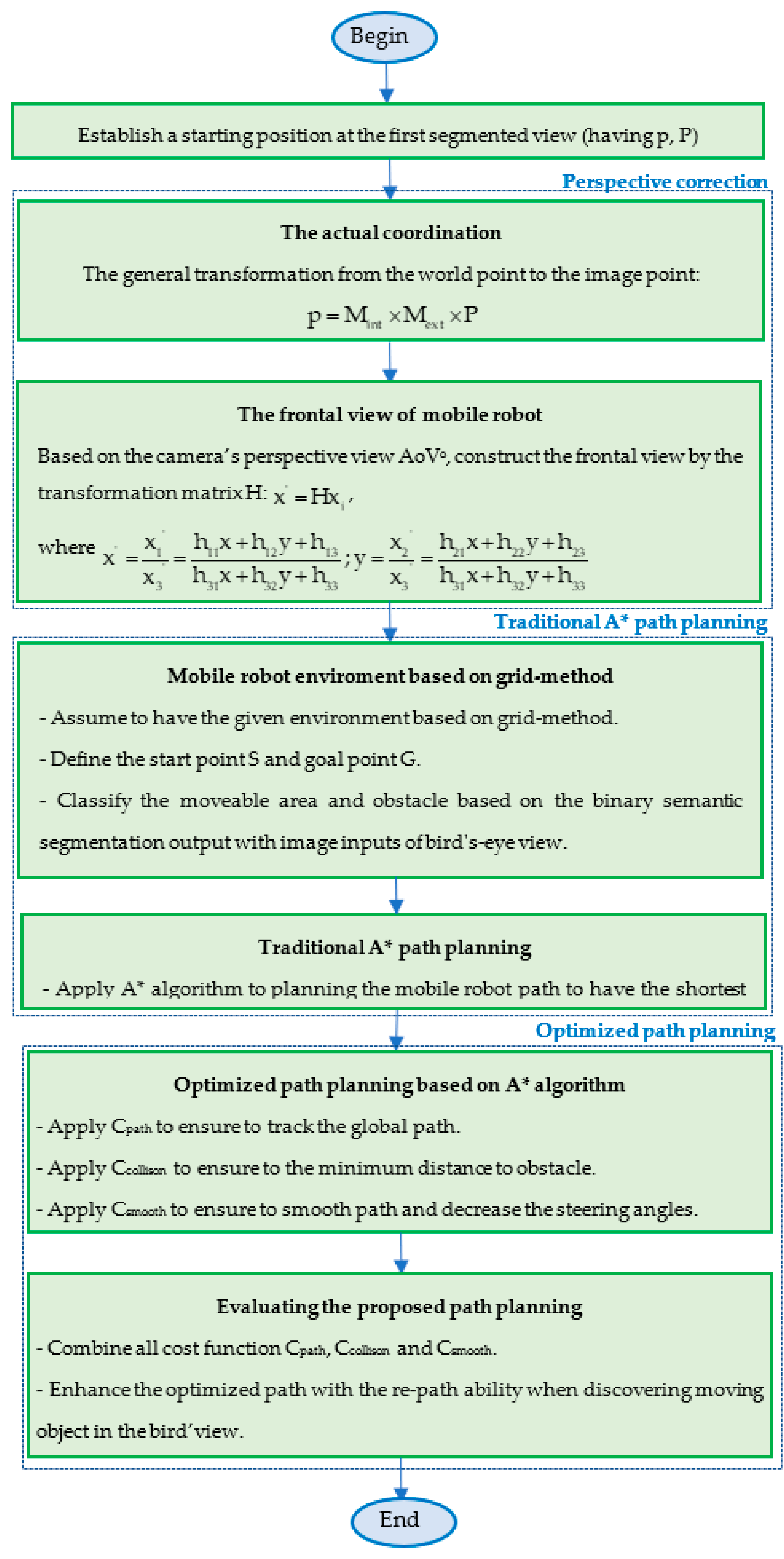
All steps of obstacle avoidance and planning strategy are according to the optimization trajectory workflow in Figure 12 as below.
4.2. Perspective Correction Process
In order to evaluate the created frontal plane, the authors will conduct studies on a checkerboard, which will provide patterns for improved recognition. In the initial experiment, the authors examine the non-obstacle region and assess the cell size in the generated image. The size of the cells in the created plane is proportionate to the size of the original cells in Figure 13. Hence, the cells in a constructed frontal plane can be utilized for qualitative measurement.
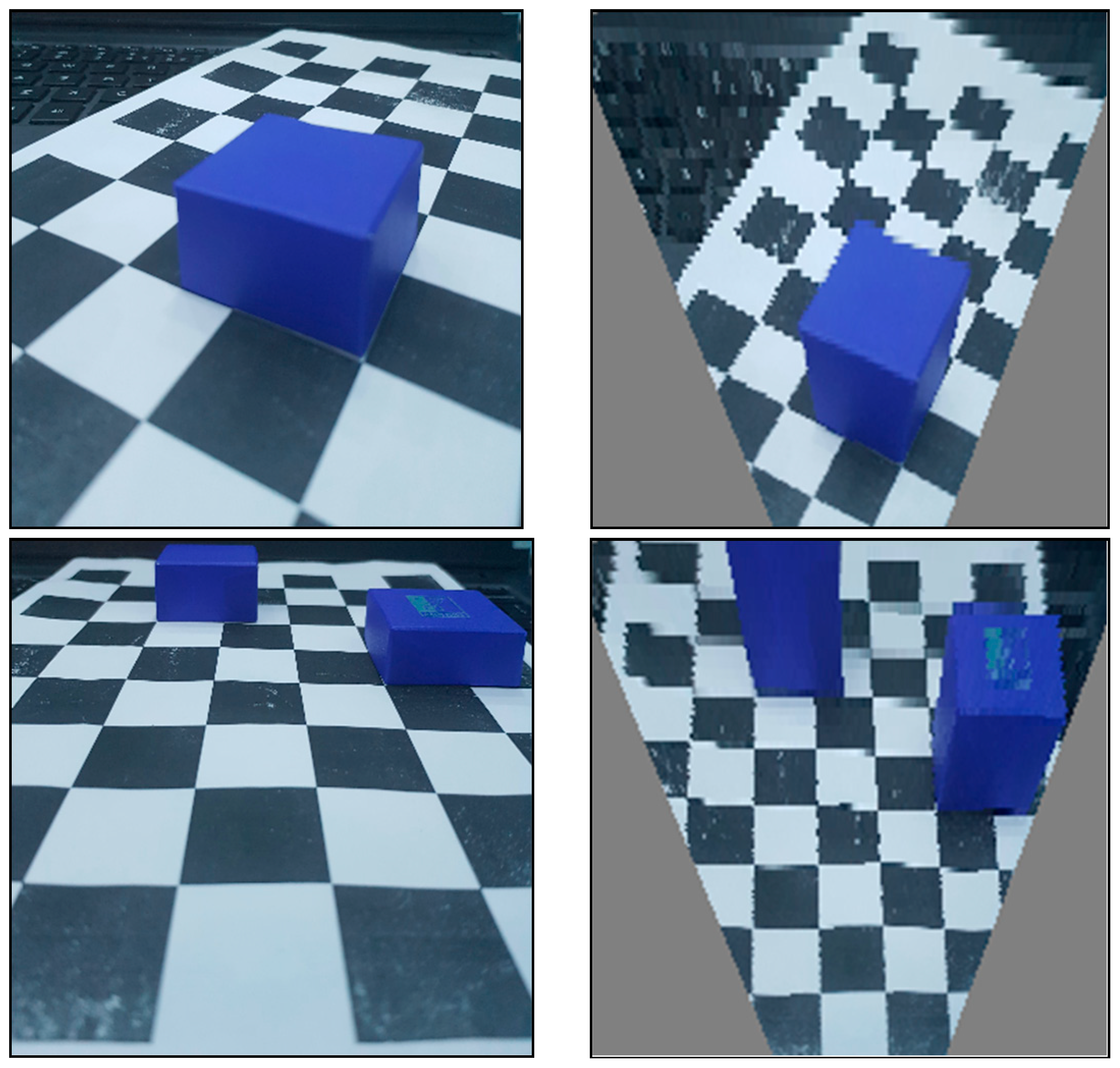
Then, the authors compare the differences between perspective correction with obstructions in various positions. Figure 14 depicts the relative position of an obstruction from an arbitrary and frontal perspective. The checkerboard cells can compare the near function while moving blocks in the checkerboard plane, observing that perspective correction is only performed to the checkerboard plane and causes an inaccuracy in the other plane.
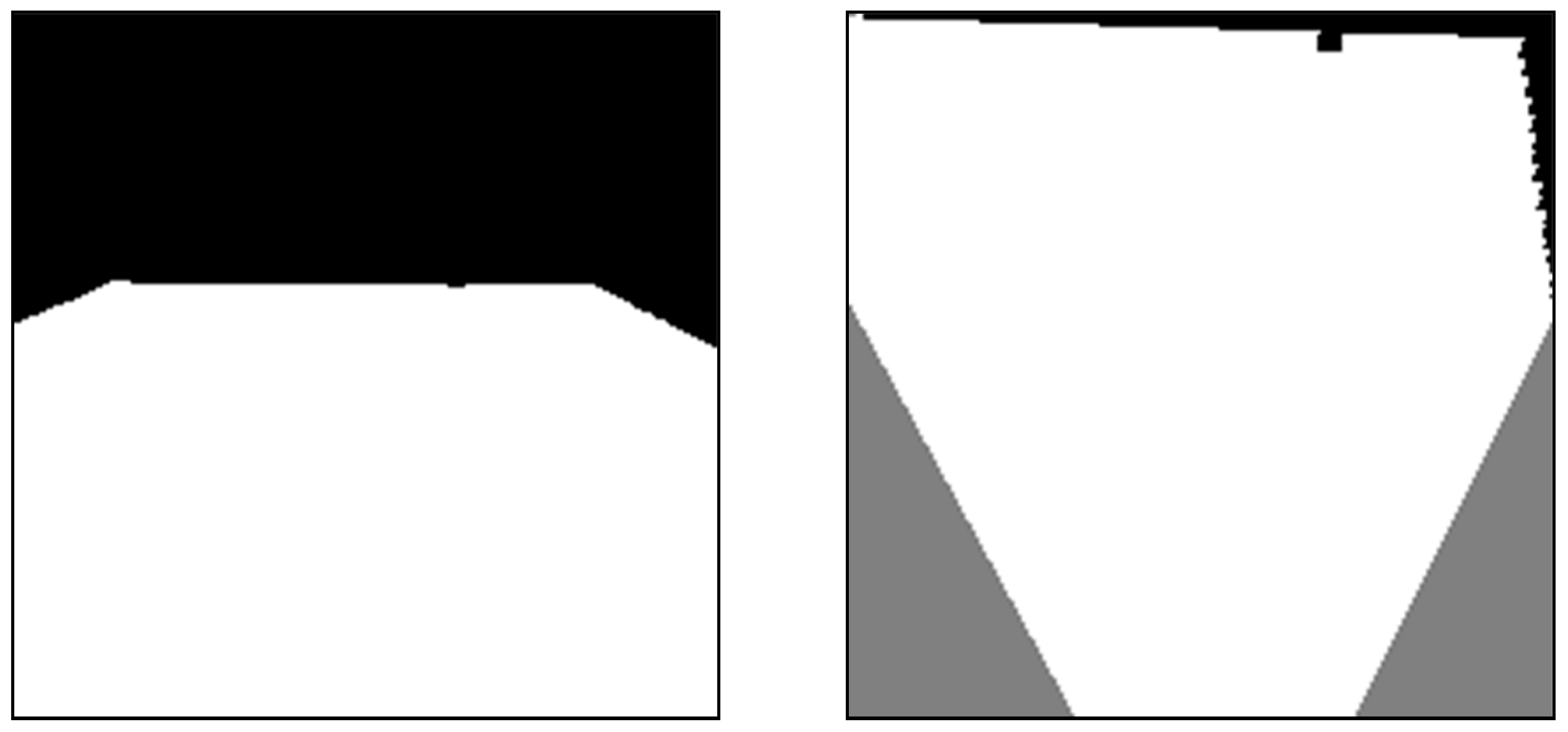
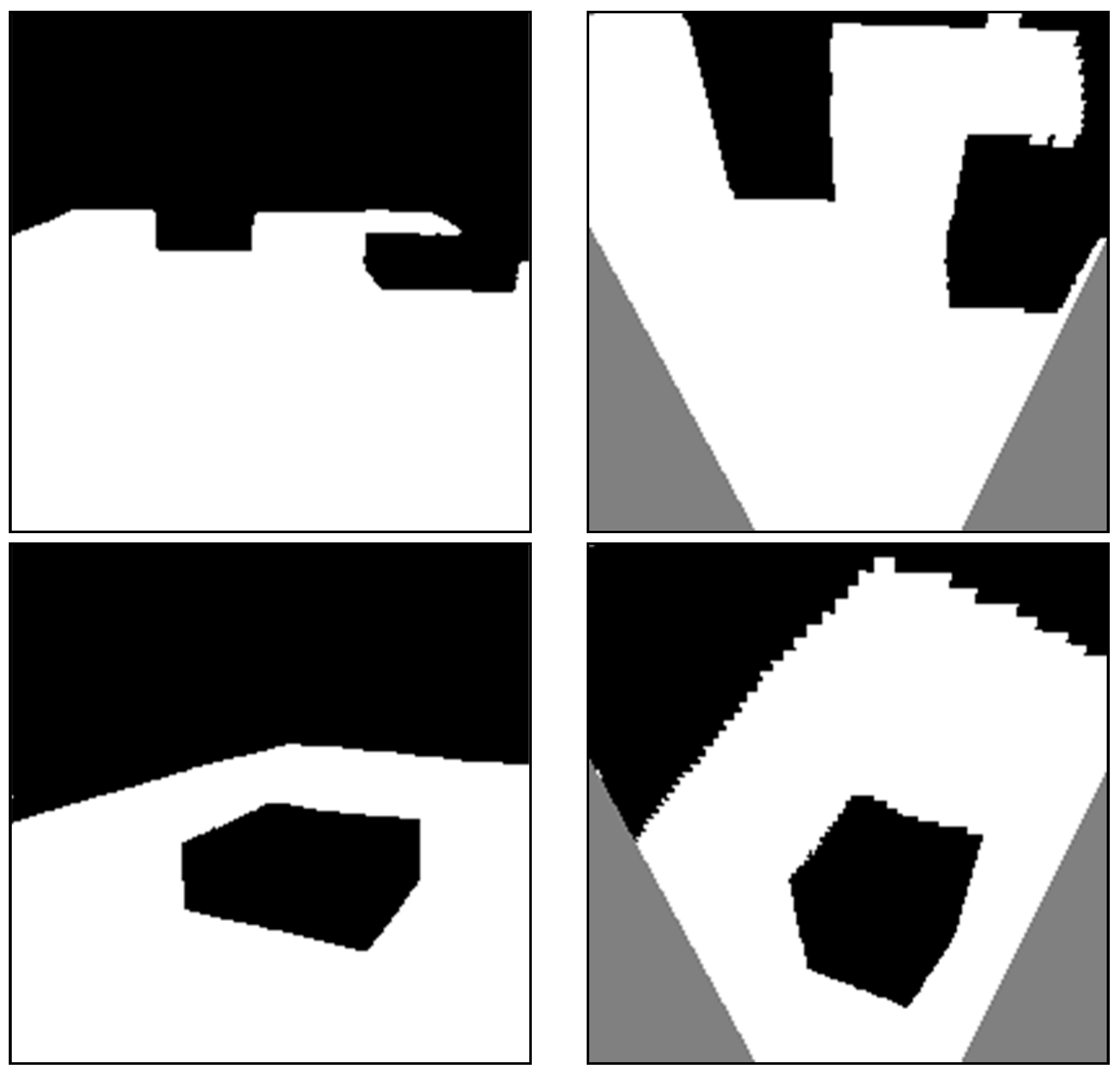
Since the authors treat the unobservable area as an unavailable area for movement, the result of perspective correction can be used to determine four different obstacle positions in Figure 15.
4.3. Path Finding Process
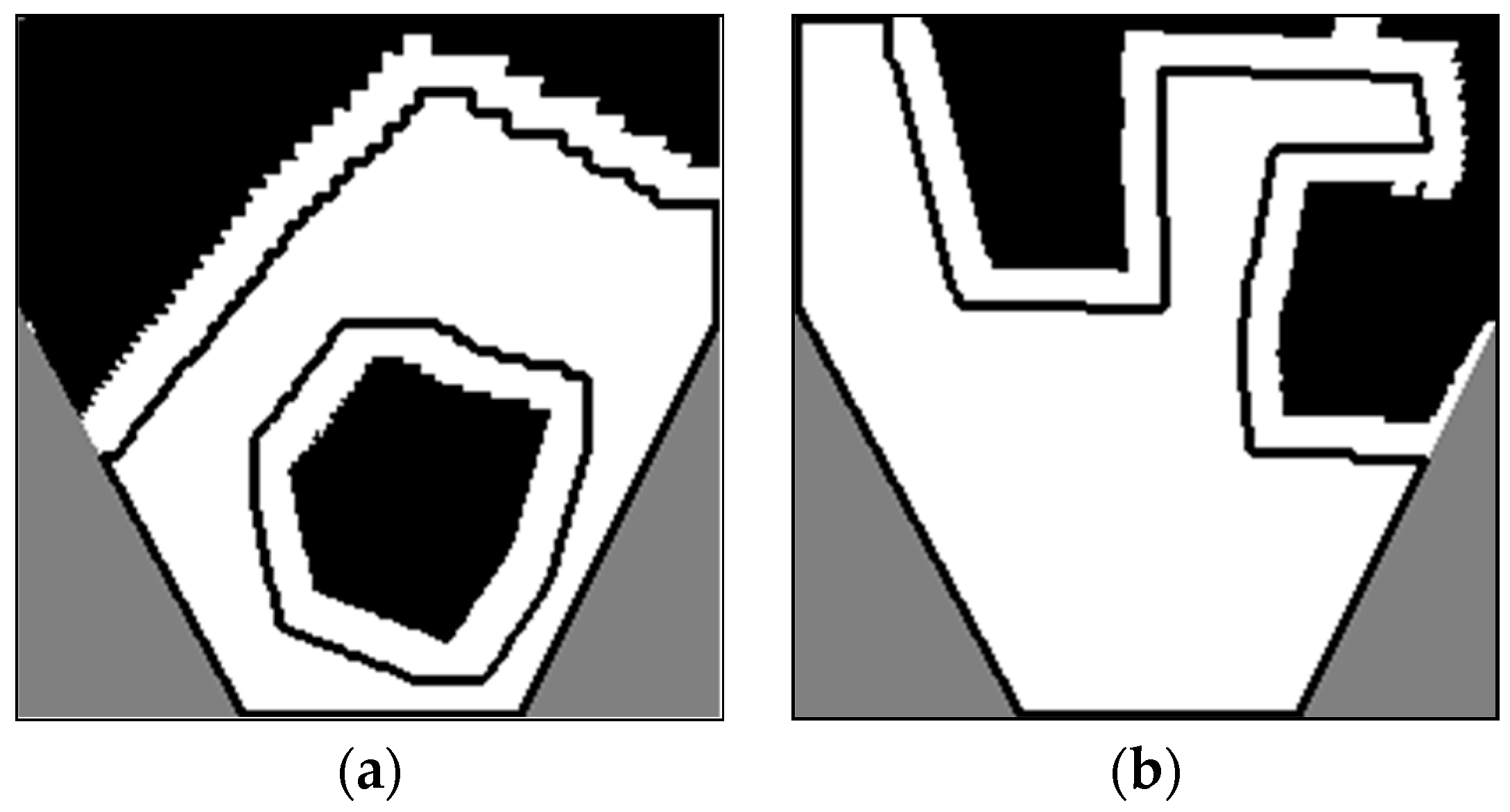
Before implementing the path finding algorithm, the authors establish the collision-free region by considering the path as a sequence of points that locate the mobile robot’s center due to the collision problem. In Figure 16, the collision-free area is delineated by extending the unusable area (black area) by a distance equal to half the mobile robot’s width. The variance in boundary dimension may result in a variable path planning outcome.
The authors apply the A* path planning algorithm to the collision-free region. As the authors plan the path on the observable area, which was rather uncomplicated in Figure 17, the computational cost of the A* algorithm is modest.
4.4. Trajectory Optimization Process
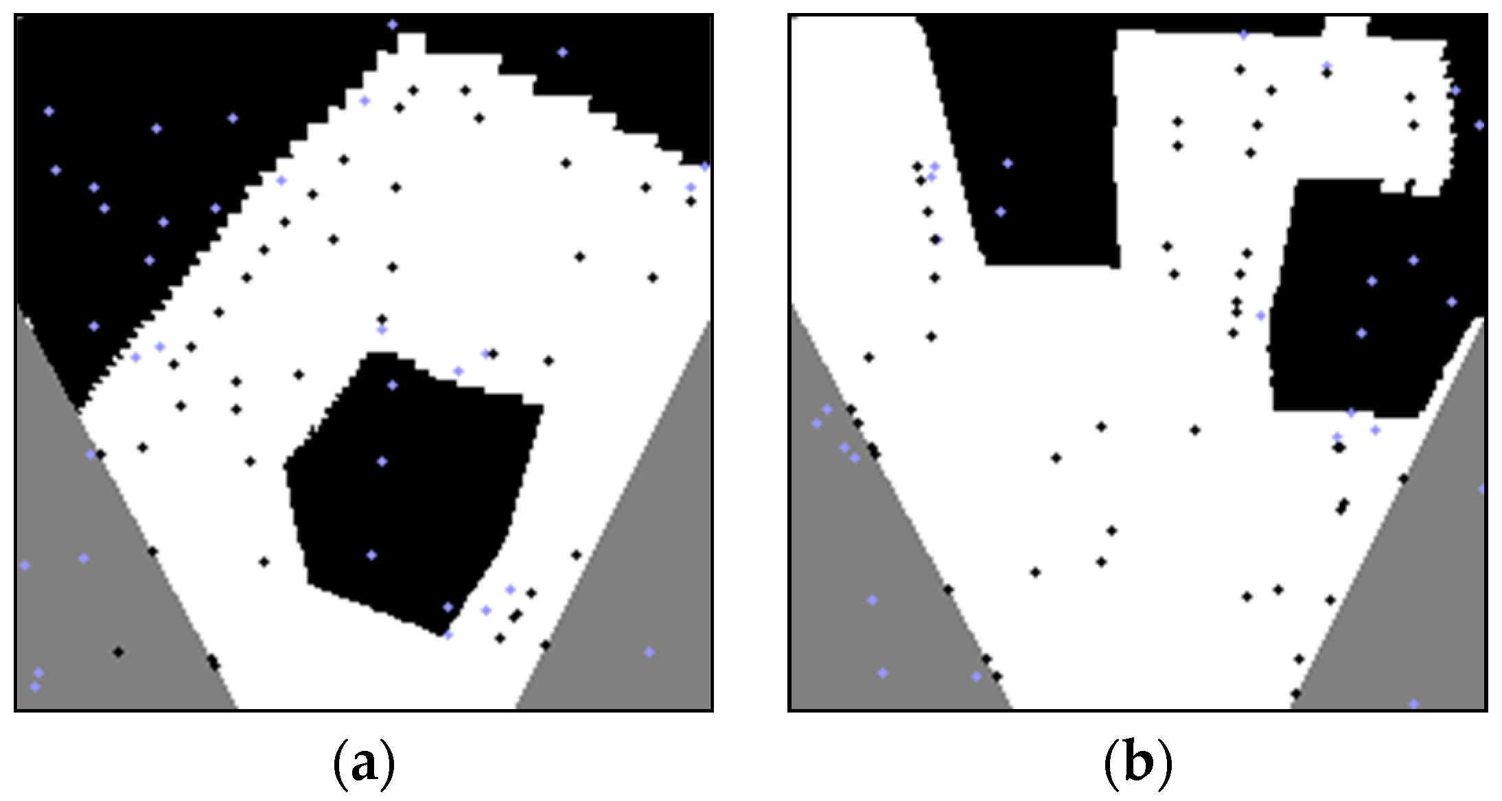
In Figure 18, the authors examine the effect of the collision cost using random blue points and the same method. The empty black spot can be used to store the blue points. There are two possible scenarios in which a mobile robot encounters barriers while moving in real time: Figure 18a depicts the environment for Scenario 1, which features a single obstacle in the bottom center, and Figure 18b depicts the environment for Scenario 2, which features a pair of obstacles at the top. To prevent accidental collisions with obstacles, Ccollision changes blue points to black ones.
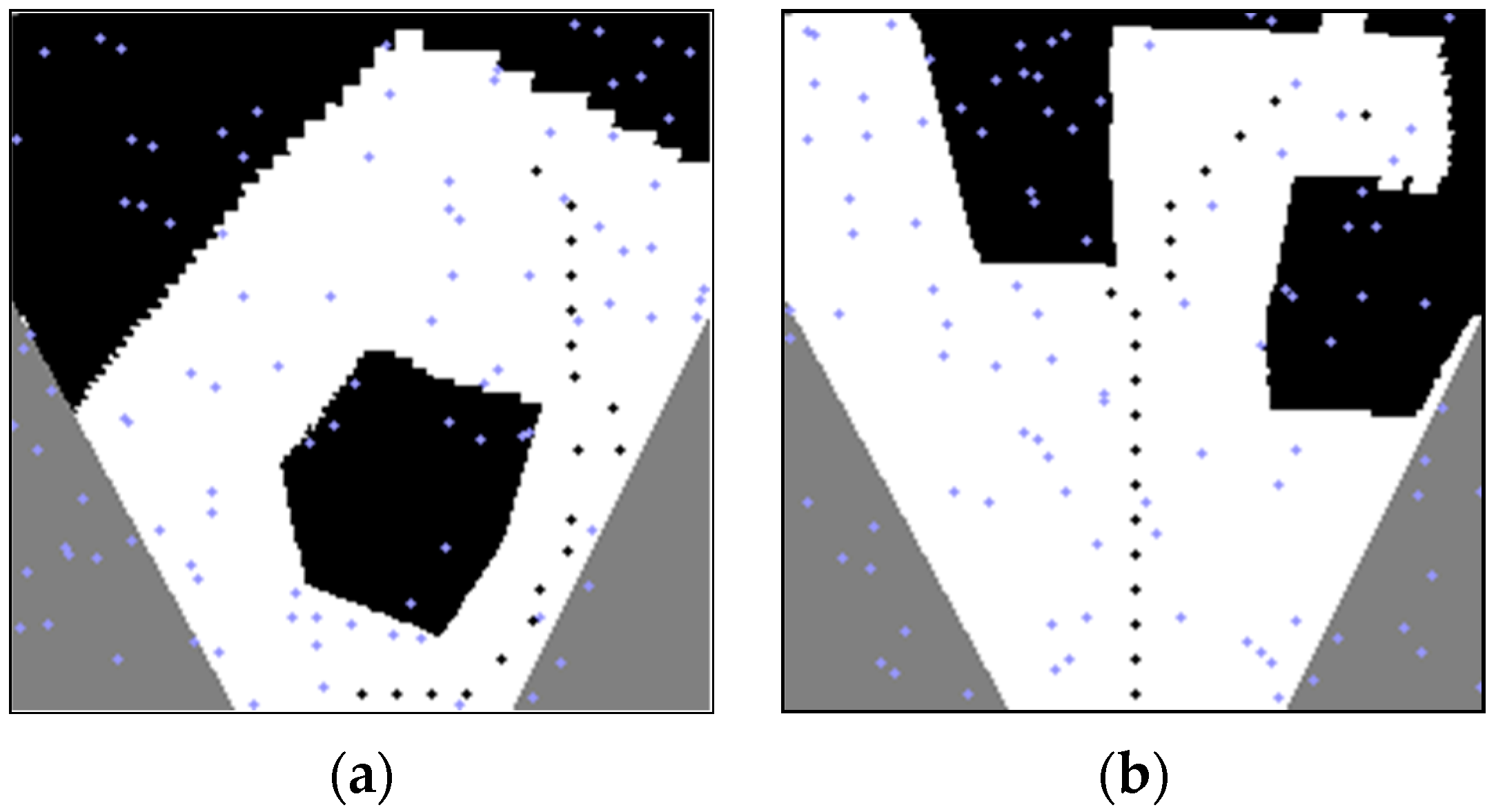
The outcome demonstrates that path cost moves random blue points to the closest points along the intended path in Figure 19.
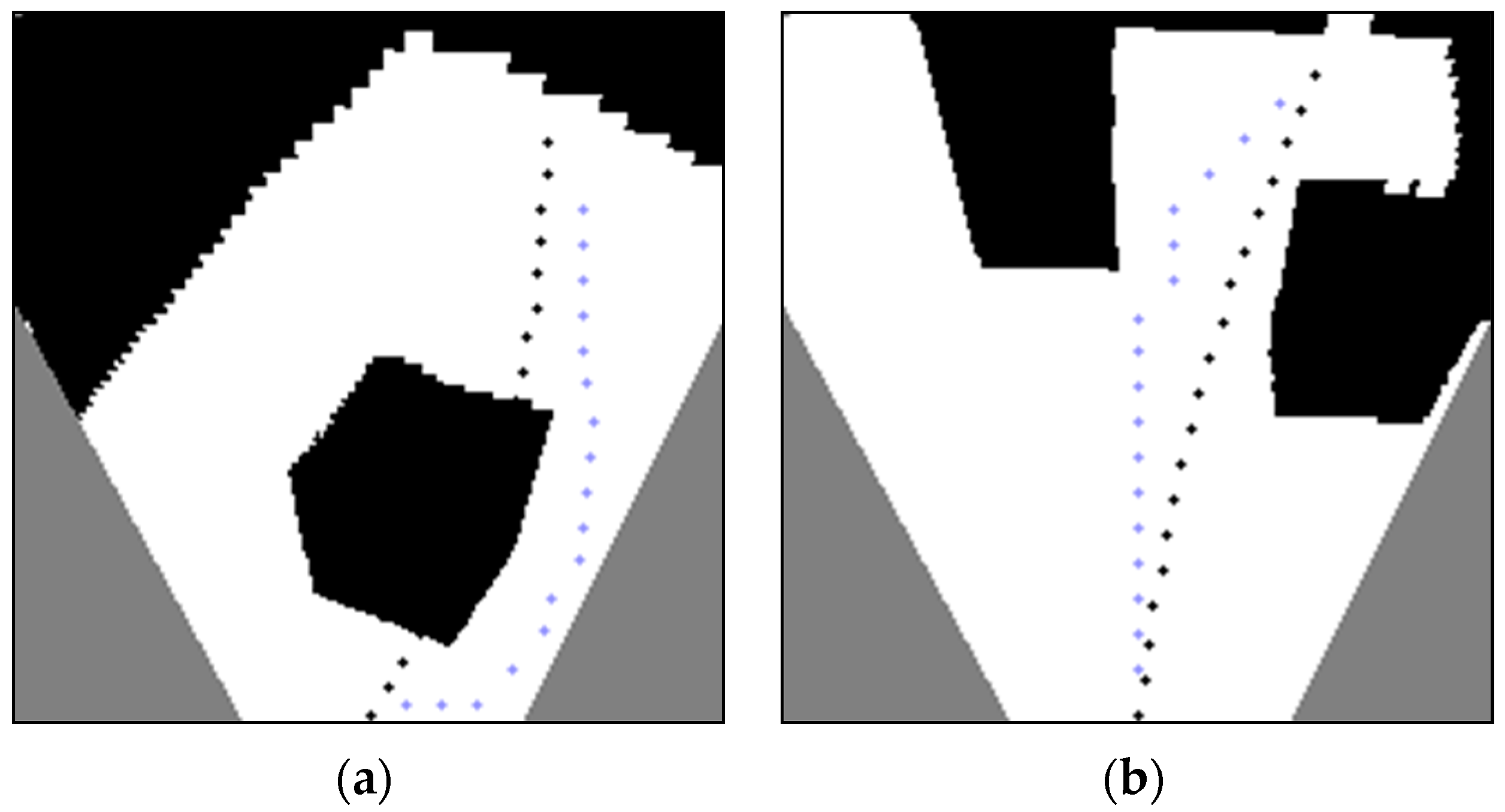
In Figure 20, a comparison is presented between the performance of the original A* path and the path generated by combining the collision cost and smooth cost. To enhance the safety of the autonomous mobile robots (AMRs), the environment is modified to ensure the path remains unobstructed, as depicted by the blue line. Including the additional collision cost in the A* heuristic cost function is a remedy for the potential issue of robot collision (indicated by the black line) when traversing or turning around an obstacle. Application of the traditional A* algorithm may not be sufficient to avoid collisions in such scenarios. Furthermore, the smooth cost decreases the angle between three consecutive path points, leading to a smoother path.
After separately studying path cost, collision cost, and smooth cost, we investigate all cost functions simultaneously and show the final results. The processing time of three scenarios is separately measured to prove the proposed path’s performance in Figure 21.
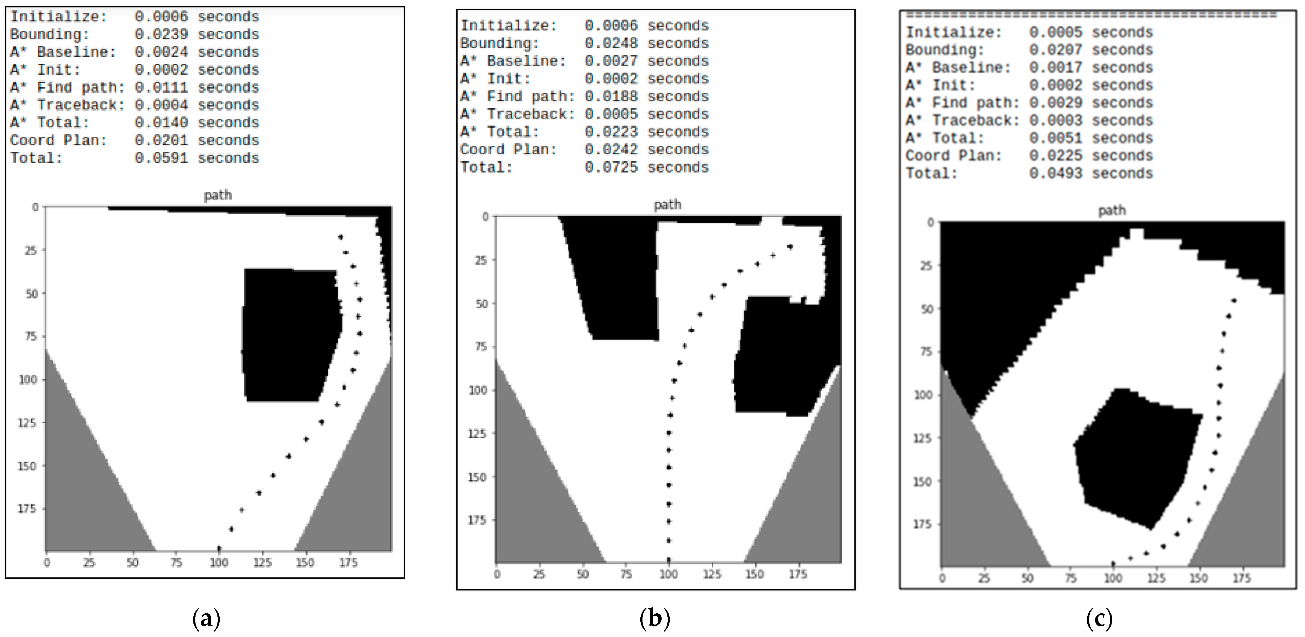
More three situations tested in the simulation are as follows: Scenario 3 has one obstacle in the top right corner of the shifting environment, whereas Scenario 4 has two, and Scenario 5 has one massive obstacle at the base. To validate the quality of the segmentation model’s design, the results are compared to those in [30]. The A* algorithm is first utilized to find the path based on optimized path planning. The overall completion time of the A* algorithm is only 0.0140, 0.0223, and 0.0051 s for Scenarios 1, 2, and 3, respectively. Finally, the enhanced A* algorithm with three cost functions, including path cost, collision cost, and smooth cost, directs the mobile robot to safely avoid obstacles and follow a smooth trajectory to its goal. In Scenario 3, the impressive processing time is 0.0591 s, in Scenario 4 it is 0.0725 s, and in Scenario 5 it is 0.0493 s.
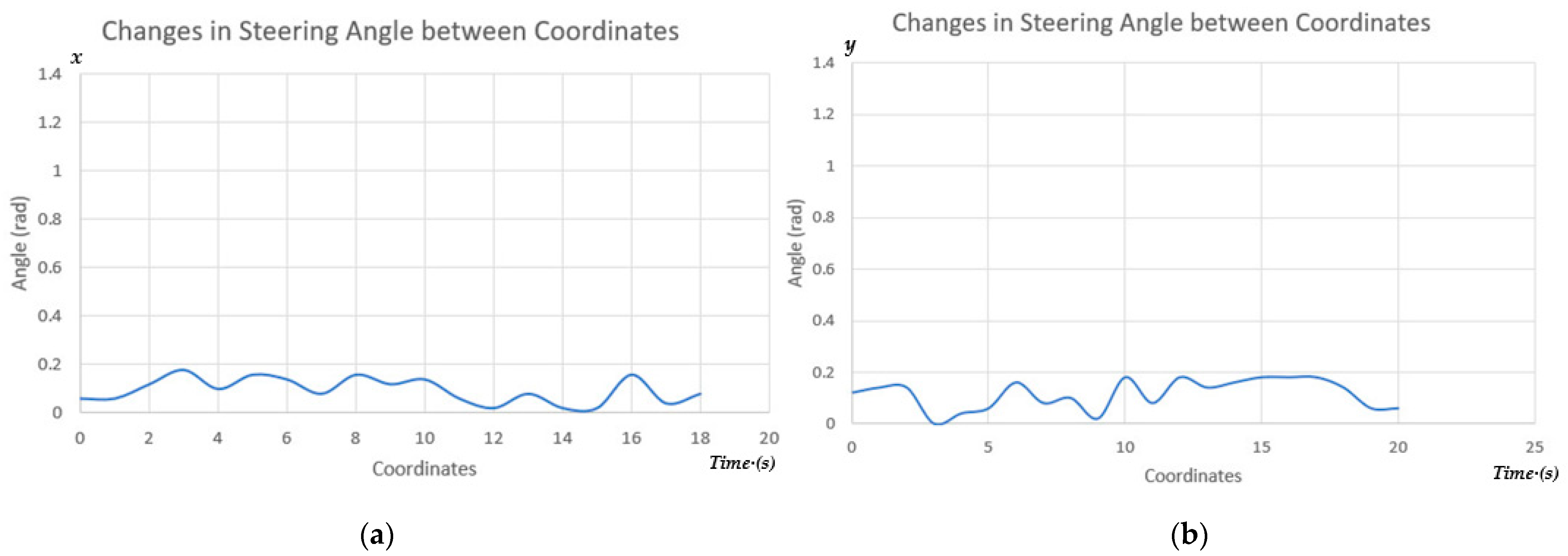
With the successful application of the optimized mobile robot navigation strategy, particularly the process of smoothing the path while maintaining the mobile robot’s safety, the tracking trajectory controlling is robust with steering angle variations of less than 0.2 rad in Figure 22.
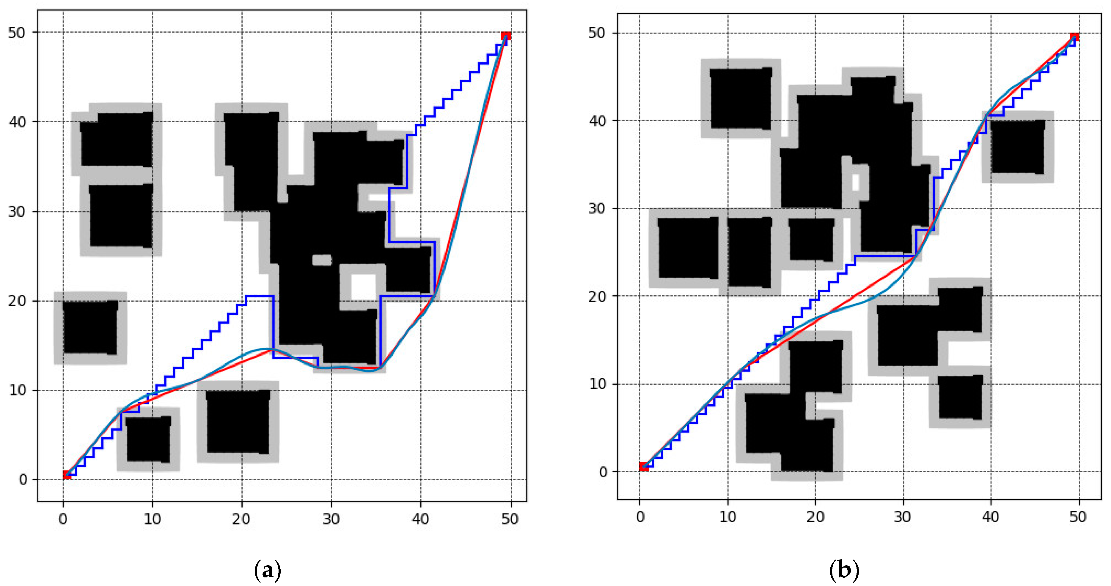
Furthermore, the authors continuously validate the mobile robot path planning performance in two continuous scenarios in Figure 23. The following 50 × 50 grid environments are continuously conducted. The start point S (0, 0) and goal point G (50, 50) were used as simulated test maps. The obstacles appeared randomly in Scenario 6, and the formation of obstacles is more complex in Scenario 7.
In both Scenarios 6 and 7, if only using A* path, the mobile robot will track only the global path and turn too many times. Hence, the A* path requires much more computational scale and memory usage. A* solution is not optimal compared with our improved A* algorithm through the path length and time processing. Furthermore, A* path moves into the serious region around the obstacle defined by collision cost (grey region) in Figure 23. Based on the binary semantic segmentation image results, using path cost and collision cost, the performance of the mobile robot path is better (red lines), in the local area of the frontal view. The path is always a collision-free distance to obstacles. Finally, when adding more smooth costs, our improved A* makes the path smoother (green lines). The trajectory must be shorter than the planning path. Table 1 displays the results of a comparison between the A* algorithm and the suggested A*-based route planning algorithm in terms of the number of path nodes and the length of the paths taken in the aforementioned two cases.
The proposed method significantly reduced the calculation path nodes and path length in the mobile robot’s movement compared to the traditional A* algorithm [17] and improved the Dijkstra algorithm [16]. Moreover, the mobile robot’s trajectory is smoother and more robust when the changed steering angle is reduced in Figure 22. In addition, the proposed path planning still ensured the shortest distance between the start and goal points. The result also consolidates the optimal mobile robot navigation strategy design.
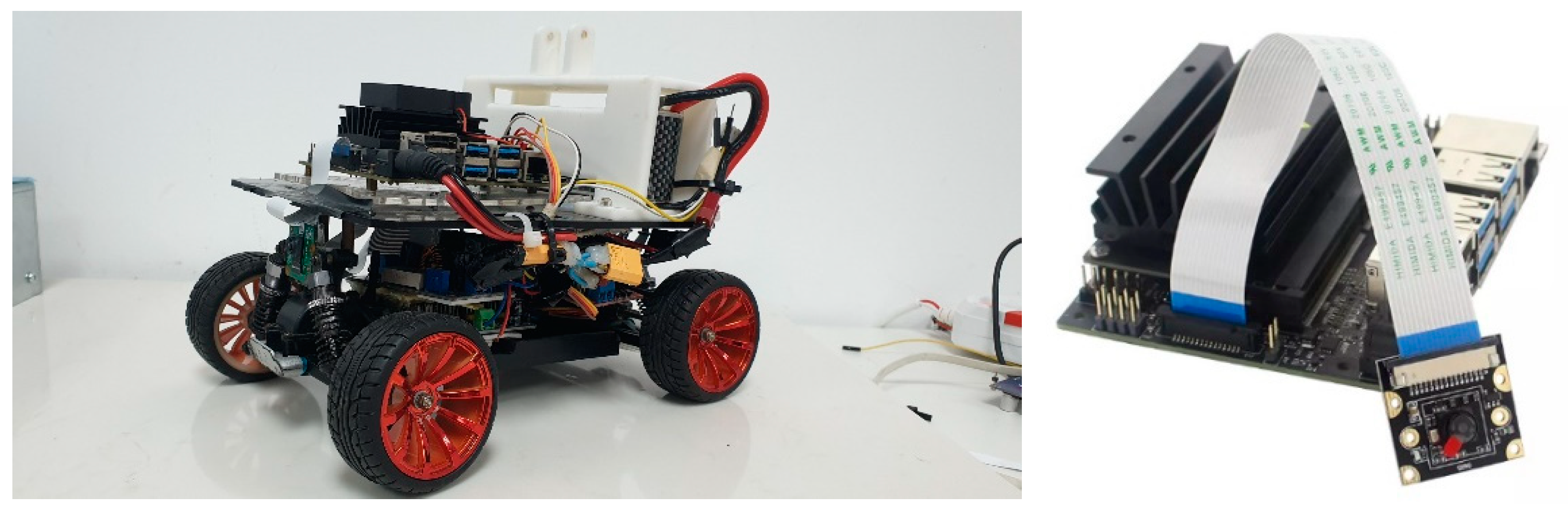
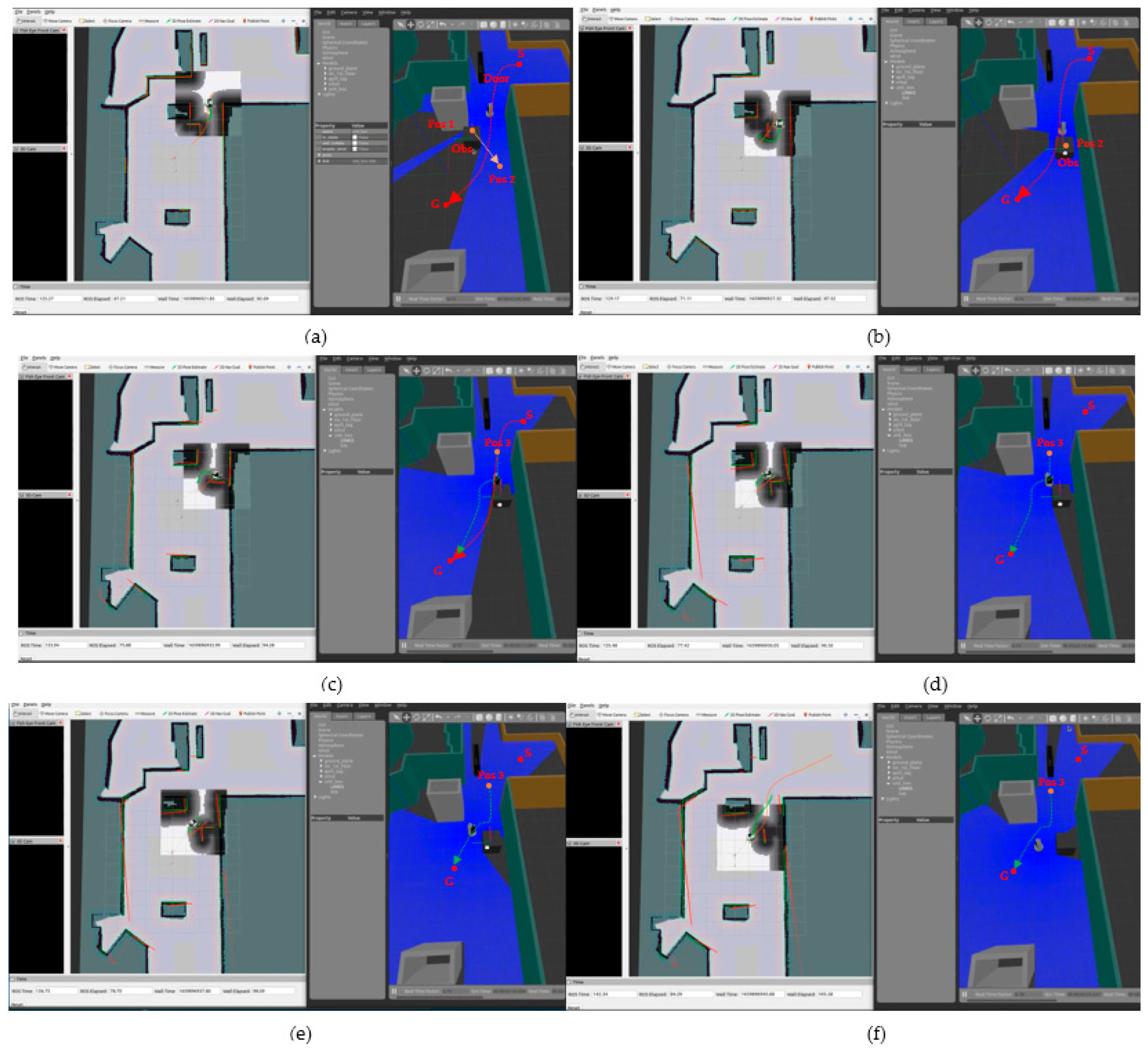
The authors will evaluate the results of the transformation and conclude that semantic segmentation is essential for constructing the frontal perspective of the ground. Then, the mobile robot’s optimal path planning can be created. Practical experimental results improve collision-free zone detecting procedures. Optimized path planning with all of the cost functions and obstacle avoidance will be created once the front view becomes the norm. Figure 24 depicts the four-wheel mobile robot used to test our proposed semantic segmentation, while Figure 25 depicts the same robot navigating a 2.8 m 1.4 m area with four obstacles in Scenario 8. Figure 25 shows how our best obstacle avoidance method [7] replans a safe global path for the mobile robot to travel along, which it then uses to move forward.
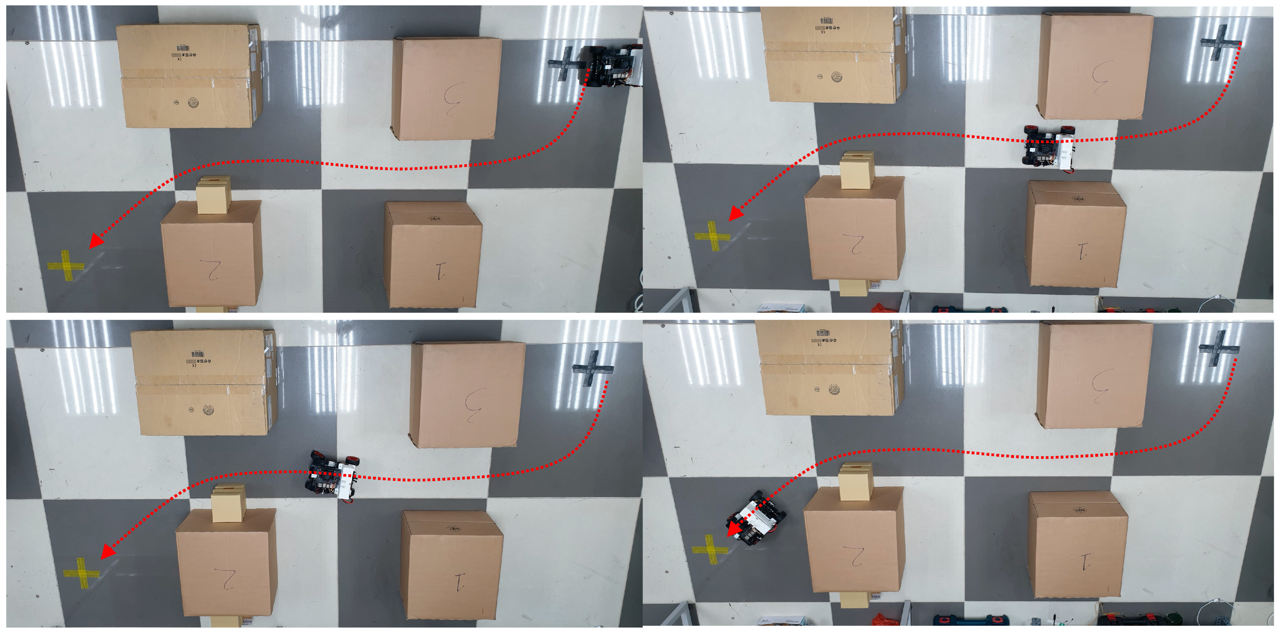
To verify the moving obstacle avoidance, the following experiments are set up in Scenario 9 under ROS environment, in Figure 26: The authors postulate a mobile robot that follows a global path from point A to point B. The obstacle Obs moved from position Pos 1 to Pos 2 with a velocity as 0.2 m/s. The mobile robot’s parameters were as follows: the maximum velocity: 1 m/s, the maximum angular velocity: 25°/s, the angular velocity resolution: 1°/s, the acceleration: 0.25 m/s2, and the angular acceleration: 45°/s2, respectively.
Figure 26 (snapshots (a)–(f)) depicts a mobile robot following a global path determined by the A* algorithm. Then, the mobile robot discovers the obstacle Obs, and the path is modified the local path to becoming the optimized path. Hence, the mobile robot avoids the obstacle successfully at Pos 1, then continues at the new Pos 2 of the moving obstacle. The experimental test is conducted on a mobile robot using the monocular camera in an actual ROS environment. In addition, the optimal mobile robot trajectory strategy ensures the mobile robot’s robust movement while avoiding obstacles. All snapshots of Figure 25 present the mobile robot’s moving process, including as follows:
In Figure 26a, at the start point S, a mobile robot will move to goal point G. The global path is entirely built. In each local area of the frontal view, the mobile robot discovers if it has obstacles in the path. Then, the mobile robot determines the door’s position and adjusts the path to move through the door successfully. Next, the mobile robot movement maintains a safe collision distance from the obstacle Obs at Pos 1, as shown in Figure 26b. Furthermore, when the obstacle moves from Pos 1 to Pos 2, the way will intersect the first global path based on the A* algorithm. In Figure 26c, if the optimized mobile robot path is not successfully implemented, the robot will collide with the obstacle Obs in Figure 26b,c (red dotted lines). The mobile robot velocity is decreased from 1 m/s to a suitable velocity to gain enough time processing of implementing the optimized path. From Figure 26d–f, the mobile robot path is completely re-planned to the new path (green dotted lines). The mobile robot successfully tracks the optimized path from S to G with a collision-free distance to the obstacle of 0.2 m. Our evaluation findings demonstrate that the method successfully detects and avoids obstacles in real time with great precision and efficiency.
5. Conclusions
Path finding in the real world necessitates multi-objective optimization issues, such as optimizing the shortest path, the smallest distance to obstacles, and the smoothest trajectory. However, obstacles may arise when the qualities of the aims contradict. Thus, a multi-objective evolutionary algorithm based on binary semantic segmentation is proposed. Furthermore, data augmentation helps predict challenging situations, such as poor lighting conditions and background clutter. The most important parts of a good obstacle avoidance algorithm are collision-free path planning, a manageable amount of processing time, and minor adjustments to the steering angle. Instead of relying on the option of following an initial reference, as with existing systems, the mobile robots’ navigation technique will be proactive in selecting flexible alternatives in the frontal view. Inputs for a perspective transform are collected from a segmentation map deemed suitable for perspective correction. From the beginning and ending locations of the map, the optimized path based on the A* algorithm will determine the direction of rapid movement.
Moreover, in the trajectory optimization process, with enhanced A* algorithm, the authors create a novel cost function construction based on the need for a path finding, collision-free path with a low steering angle. Collision cost Ccollision prevents collisions caused by penalty points in inaccessible regions and moves them to the nearest available region. Path cost Cpath ensures the continuity of the series of coordinates by assigning penalty points when the path deviates from its intended course. Finally, the expense is streamlined. Csmooth decreases the steering angle by penalizing the distance between three consecutive points. After separately studying each component, the authors integrate the cost function and produce the final results. Authors measure the impressive processing time at each phase to evaluate the performance process and trajectory quality. A mobile robot can move stable and robots with the steering angle variations less than 0.2 rad. The simulation outcomes satisfactorily demonstrate the accuracy and enhancement of the proposed strategy. Our long-term objective is to train the model to distinguish between many different types of interior obstructions by using data from multiple classes. As a result, path planning will function better in a wide range of indoor environments. In addition, the gathered data could be used with sensor systems to deal with intricate issues in the global and local outside environment.
Author Contributions
Conceptualization, T.-V.D. and N.-T.B.; Project Administration, T.-V.D.; Supervision, N.-T.B.; Funding Acquisition: N.-T.B.; Methodology, T.-V.D. and N.-T.B.; Formal Analysis, N.-T.B.; Software, T.-V.D.; Experimental data and system, T.-V.D.; Writing—Review and Editing, T.-V.D. and N.-T.B. All authors have read and agreed to the published version of the manuscript.
Funding
This work was supported by the Centennial SIT Action for the 100th anniversary of Shibaura Institute of Technology entering the top 10 at the Asian Institute of Technology.
Data Availability Statement
The data that support the findings of this study are available on request from the corresponding author, Thai-Viet Dang.
Acknowledgments
The authors express grateful thankfulness to Vietnam-Japan International Institute for Science of Technology (VJIIST), School of Mechanical Engineering, HUST, Vietnam and Shibaura Institute of Technology, Japan.
Conflicts of Interest
The authors declare no conflict of interest.
References
- Raghuvanshi, D.S.; Dutta, I.; Vaidya, R.J. Design and analysis of a novel sonar-based obstacle avoidance system for the visually impaired and unmanned systems. In Proceedings of the International Conference on Embedded Systems (ICES), Coimbatore, India, 3–5 July 2014. [Google Scholar]
- Al-Mallah, M.; Ali, M.; Al-Khawaldeh, M. Obstacles Avoidance for Mobile Robot Using Type-2 Fuzzy Logic Controller. Robotics 2022, 11, 130. [Google Scholar] [CrossRef]
- Murat, L.; Ertugrul, C.; Faruk, U.; Ibrahim, U.; Salih, I.A. Initial Results of Testing a Multilayer Laser Scanner in a Collision Avoidance System for Light Rail Vehicles. Appl. Sci. 2018, 8, 475. [Google Scholar]
- Wang, W.C.; Ng, C.Y.; Chen, R. Vision-Aided Path Planning Using Low-Cost Gene Encoding for a Mobile Robot. Intell. Automat. Soft Comput. 2021, 32, 991–1007. [Google Scholar] [CrossRef]
- Castilloa, G.D.; Skaar, S.; Cardenasb, A.; Fehrc, L. A sonar approach to obstacle detection for a vision-based autonomous wheelchair. Robot. Auton. Syst. 2006, 54, 967–981. [Google Scholar] [CrossRef]
- Abukhalil, T.; Alksasbeh, M.; Alqaralleh, B.; Abukaraki, A. Robot navigation system using laser and monocular camera. J. Theor. Appl. Inf. Technol. 2020, 98, 714–724. [Google Scholar]
- Dang, T.V.; Bui, N.T. Multi-Scale Fully Convolutional Network-Based Semantic Segmentation for Mobile Robot Navigation. Electronics 2023, 12, 533. [Google Scholar] [CrossRef]
- Zhao, C.Q.; Sun, Q.Y.; Zhang, C.Z.; Tang, Y.; Qian, F. Monocular depth estimation based on deep learning: An overview. Sci. China Technol. Sci. 2020, 63, 1612–1627. [Google Scholar] [CrossRef]
- Dong, Q. Path Planning Algorithm Based on Visual Image Feature Extraction for Mobile Robots. Mob. Inf. Syst. 2022, 2022, 4094472. [Google Scholar] [CrossRef]
- Minaee, S.; Boykov, Y.Y.; Porikli, F.; Plaza, A.J.; Kehtarnavaz, N.; Terzopoulos, D. Image Segmentation Using Deep Learning: A Survey. IEEE Trans. Pattern Anal. Mach. Intell. 2022, 44, 3523–3542. [Google Scholar] [CrossRef]
- Li, B.; Shi, Y.; Qi, Z.; Chen, Z. A Survey on Semantic Segmentation. In Proceedings of the 2018 IEEE International Conference on Data Mining Workshops (ICDMW), Singapore, 17–20 November 2018; pp. 1233–1240. [Google Scholar]
- Li, L.; Zhang, W.; Zhang, X.; Emam, M.; Jing, W. Semi-Supervised Remote Sensing Image Semantic Segmentation Method Based on Deep Learning. Electronics 2023, 12, 348. [Google Scholar] [CrossRef]
- Yanga, D.; Du, Y.; Yaoa, H.; Bao, L. Image semantic segmentation with hierarchical feature fusion based on deep neural network. Connect. Sci. 2022, 34, 1772–1784. [Google Scholar] [CrossRef]
- Fusic, S.J.; Hariharan, K.; Sitharthan, R.; Karthikeyan, S. Scene terrain classification for autonomous vehicle navigation based on semantic segmentation method. Trans. Inst. Meas. Control 2022, 44, 2574–2589. [Google Scholar] [CrossRef]
- Gharajeh, M.S.; Jond, H.B. An Intelligent Approach for Autonomous Mobile Robots Path Planning Based on Adaptive Neuro-fuzzy Inference System. Ain Shams Eng. J. 2022, 13, 101491. [Google Scholar] [CrossRef]
- Alshammrei, S.; Boubaker, S.; Kolsi, L. Improved Dijkstra Algorithm for Mobile Robot Path Planning and Obstacle Avoidance. Comput. Mater. Contin. 2022, 72, 5939–5954. [Google Scholar] [CrossRef]
- Xunyu, Z.; Jun, T.; Huosheng, H.; Xiafu, P. Hybrid Path Planning Based on Safe A* Algorithm and Adaptive Window Approach for Mobile Robot in Large-Scale Dynamic Environment. J. Intell. Robot. Syst. 2020, 99, 65–77. [Google Scholar]
- Eshtehardian, S.A.; Khodaygan, S. A continuous RRT*-based path planning method for non-holonomic mobile robots using B-spline curves. J. Ambient. Intell. Humaniz. Comput. 2022. [Google Scholar] [CrossRef]
- Masato, K.; Naoki, M. Local Path Planning: Dynamic Window Approach with Virtual Manipulators Considering Dynamic Obstacles. IEEE Access 2022, 10, 17018–17029. [Google Scholar]
- Nguyen, L.V.; Phung, M.D.; Ha, Q.P. Game Theory-Based Optimal Cooperative Path Planning for Multiple UAVs. IEEE Access 2022, 10, 108034–108045. [Google Scholar] [CrossRef]
- Wang, W.; Zhao, J.; Li, Z.; Huang, J. Smooth Path Planning of Mobile Robot Based on Improved Ant Colony Algorithm. J. Robot. 2021, 2021, 4109821. [Google Scholar] [CrossRef]
- Goldenberg, M. The Heuristic Search Research Framework. Knowl. Based Syst. 2017, 129, 1–3. [Google Scholar] [CrossRef]
- Li, Y.; Jin, R.; Xu, X.; Qian, Y.; Wang, H.; Xu, S.; Wang, Z. A Mobile Robot Path Planning Algorithm Based on Improved A∗ Algorithm and Dynamic Window Approach. IEEE Access 2022, 10, 57736–57747. [Google Scholar] [CrossRef]
- Daniel, A.; Chinnappan, C.V.; Muthu, B.A.; Kumar, R.S.; Sivaparthipan, C.B.; Marin, C.E.M. Fully convolutional neural networks for LIDAR–camera fusion for pedestrian detection in autonomous. Multimed. Tools Appl. 2023. [CrossRef]
- Agus, E.M.; Bagas, Y.S.; Yuda, M.; Hanung, A.N.; Zaidah, I. Convolutional Neural Network featuring VGG-16 Model for Glioma Classification. Int. J. Inform. Vis. 2022, 6, 660–666. [Google Scholar] [CrossRef]
- Elhawary, H.M.; Shapiaib, M.I.; Elfakharany, A. Investigation on the Effect of the Feature Extraction Backbone for Small Object Segmentation using Fully Convolutional Neural Network in Traffic Signs Application. IOP Conf. Ser. Mater. Sci. Eng. 2021, 1051, 012006. [Google Scholar] [CrossRef]
- Shelhamer, E.; Long, J.; Darrell, T. Fully convolutional networks for semantic segmentation. IEEE Trans. Pattern Anal. Mach. Intell. 2017, 39, 640–651. [Google Scholar] [CrossRef]
- Yang, S.; Maturana, D.; Scherer, S. Realtime 3D scene layout from a single image using convolutional neural networks. In Proceedings of the 2016 IEEE International Conference on Robotics and Automation (ICRA), Stockholm, Sweden, 16–21 May 2016; pp. 2183–2189. [Google Scholar]
- Lafferty, J.; Mccallum, A.; Pereira, F. Conditional Random Fields: Probabilistic Models for Segmenting and Labeling Sequence Data. In Proceedings of the 18th International Conference on Machine Learning, San Francisco, CA, USA, 28 June–1 July 2001. [Google Scholar]
- Oršic’, M.; Šegvic, S. Efficient semantic segmentation with pyramidal fusion. Pattern Recognit. 2021, 110, 107611. [Google Scholar] [CrossRef]
- Hartley, R.; Xisserman, A. Multiple View Geometry in Computer Vision; Cambridge University Press: Cambridge, UK, 2000. [Google Scholar]
- Kim, D.; Fessler, J.A. On the Convergence Analysis of the Optimized Gradient Method. J. Optim. Theory Appl. 2017, 172, 187–205. [Google Scholar] [CrossRef]
Figure 1.
Multi-scale fully convolutional network [27].
Figure 1.
Multi-scale fully convolutional network [27].

Figure 2.
Ground truth and prediction in the loss function (BCE).

Figure 3.
Training and validation on training images using mean intersection over union—mIoU as metric: (a) VGG-FCNs-CMU-96 × 96; (b) VGG-FCNs-Augment-96 × 96.
Figure 3.
Training and validation on training images using mean intersection over union—mIoU as metric: (a) VGG-FCNs-CMU-96 × 96; (b) VGG-FCNs-Augment-96 × 96.

Figure 4.
Segmentation results of the Ta Quang Buu library’s environment: (a) raw images; (b) ground truths; and (c) predictions.
Figure 4.
Segmentation results of the Ta Quang Buu library’s environment: (a) raw images; (b) ground truths; and (c) predictions.

Figure 5.
Result of semantic segmentation process.

Figure 6.
A projective transformation is defined by four points on the scene plane: (a) any four points arbitrary view of an environment’s image, and (b) four points in the frontal view after using a projective transformation.
Figure 6.
A projective transformation is defined by four points on the scene plane: (a) any four points arbitrary view of an environment’s image, and (b) four points in the frontal view after using a projective transformation.

Figure 7.
The checker board and the frontal view.

Figure 8.
Source image and constructed frontal plane.

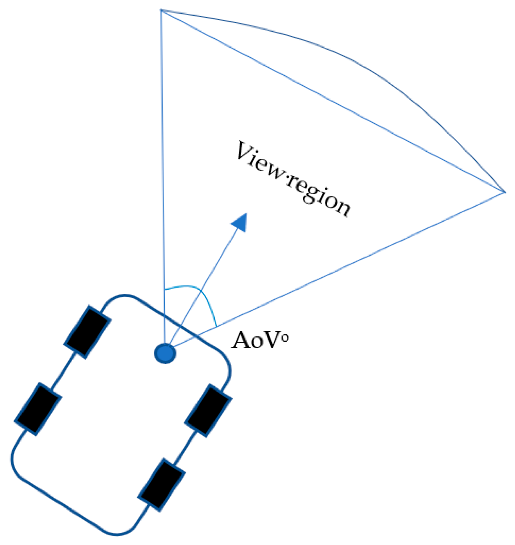
Figure 9.
The mobile robot’s bird view.

Figure 10.
Detect collision-free area and cells division.

Figure 11.
Symmetric path search: (a) four search directions of neighborhood; (b) eight search directions of neighborhood.
Figure 11.
Symmetric path search: (a) four search directions of neighborhood; (b) eight search directions of neighborhood.

Figure 12.
The optimization trajectory workflow.

Figure 13.
Perspective correction on checkerboard.

Figure 14.
Relative obstacle position in frontal plane with four different obstacle positions.

Figure 15.
Perspective correction in semantic segmentation image with four different obstacle positions.
Figure 15.
Perspective correction in semantic segmentation image with four different obstacle positions.

Figure 16.
Determine the bounding of the collision-free area: (a) having one obstacle at the bottom of the environment, (b) having two obstacles at the top of the environment.
Figure 16.
Determine the bounding of the collision-free area: (a) having one obstacle at the bottom of the environment, (b) having two obstacles at the top of the environment.

Figure 17.
Path planning in the collision-free area in the conventional A* path: (a) having one obstacle at the bottom of the environment, (b) having two obstacles at the top of the environment.
Figure 17.
Path planning in the collision-free area in the conventional A* path: (a) having one obstacle at the bottom of the environment, (b) having two obstacles at the top of the environment.

Figure 18.
Effect of the collision cost Ccollision in the enhanced A* path: (a) having one obstacle at the bottom of the environment, (b) having two obstacles at the top of the environment.
Figure 18.
Effect of the collision cost Ccollision in the enhanced A* path: (a) having one obstacle at the bottom of the environment, (b) having two obstacles at the top of the environment.

Figure 19.
Effect of the path cost Cpath in the enhanced A* path: (a) having one obstacle at the bottom of the environment, (b) having two obstacles at the top of the environment.
Figure 19.
Effect of the path cost Cpath in the enhanced A* path: (a) having one obstacle at the bottom of the environment, (b) having two obstacles at the top of the environment.

Figure 20.
Effect of the smooth cost in the enhanced A* path: (a) having one obstacle at the bottom of the environment, (b) having two obstacles at the top of the environment.
Figure 20.
Effect of the smooth cost in the enhanced A* path: (a) having one obstacle at the bottom of the environment, (b) having two obstacles at the top of the environment.

Figure 21.
Final trajectory results with real-time measurement: (a) having one obstacle at the top right of the environment, (b) having two obstacles at the top of the environment, and (c) having one obstacle at the bottom of the environment.
Figure 21.
Final trajectory results with real-time measurement: (a) having one obstacle at the top right of the environment, (b) having two obstacles at the top of the environment, and (c) having one obstacle at the bottom of the environment.

Figure 22.
Changes in steering angle while mobile robot is tracking optimal trajectory: (a) steering angle between coordinates in x axis, (b) steering angle between coordinates in y axis.
Figure 22.
Changes in steering angle while mobile robot is tracking optimal trajectory: (a) steering angle between coordinates in x axis, (b) steering angle between coordinates in y axis.

Figure 23.
Mobile robot path using traditional A* algorithm (blue lines), our improved A* algorithm without smooth cost (red lines), and our improved A* algorithm with all cost functions (green lines): (a) Scenario 6 with random obstacles and (b) Scenario 7 with more complex obstacles.
Figure 23.
Mobile robot path using traditional A* algorithm (blue lines), our improved A* algorithm without smooth cost (red lines), and our improved A* algorithm with all cost functions (green lines): (a) Scenario 6 with random obstacles and (b) Scenario 7 with more complex obstacles.

Figure 24.
Jetson nano-powered mobile robot with 8-megapixel Raspberry Pi camera module.

Figure 25.
Mobile robot path in experimental four obstacles scenarios.

Figure 26.
Optimized trajectory of mobile robot in the experimental moving obstacle scenario in ROS environment with the global path is dotted red lines and the re-path is dotted green lines: (a) Mobile robot moves from the start point S to goal point G, through the gate and avoid the obstacle Obs at Pos 1 (red dotted line); (b) After avoiding the obstacle Obs, mobile robot detect the moving obstacle at Pos 2; (c) The path is changed to ensure the moving obstacle Obs (green dotted line); (d) mobile robot moves successfully according to a new re-path; (e) mobile robot turn left to avoid the conner of the moving Obs; (f) mobile robot reaches to the goal point G with new re-path.


Disclaimer/Publisher’s Note: The statements, opinions and data contained in all publications are solely those of the individual author(s) and contributor(s) and not of MDPI and/or the editor(s). MDPI and/or the editor(s) disclaim responsibility for any injury to people or property resulting from any ideas, methods, instructions or products referred to in the content. |
© 2023 by the authors. Licensee MDPI, Basel, Switzerland. This article is an open access article distributed under the terms and conditions of the Creative Commons Attribution (CC BY) license (https://creativecommons.org/licenses/by/4.0/).
Share and Cite
MDPI and ACS Style
Dang, T.-V.; Bui, N.-T. Obstacle Avoidance Strategy for Mobile Robot Based on Monocular Camera. Electronics 2023, 12, 1932. https://doi.org/10.3390/electronics12081932
AMA Style
Dang T-V, Bui N-T. Obstacle Avoidance Strategy for Mobile Robot Based on Monocular Camera. Electronics. 2023; 12(8):1932. https://doi.org/10.3390/electronics12081932
Chicago/Turabian StyleDang, Thai-Viet, and Ngoc-Tam Bui. 2023. "Obstacle Avoidance Strategy for Mobile Robot Based on Monocular Camera" Electronics 12, no. 8: 1932. https://doi.org/10.3390/electronics12081932
Note that from the first issue of 2016, this journal uses article numbers instead of page numbers. See further details here.