


Multi-Mode Data Generation and Fault Diagnosis of Bearings Based on STFT-SACGAN

State Key Laboratory of Mechanics and Control for Aerospace Structures, Nanjing University of Aeronautics and Astronautics, Nanjing 210016, China
*
Authors to whom correspondence should be addressed.
Electronics 2023, 12(8), 1910; https://doi.org/10.3390/electronics12081910
Submission received: 28 March 2023
/
Revised: 14 April 2023
/
Accepted: 17 April 2023
/
Published: 18 April 2023
(This article belongs to the Topic Machine and Deep Learning)
Abstract
:To achieve multi-mode fault sample generation and fault diagnosis of bearings in a complex operating environment with scarce labeled data. Combining a semi-supervised generative adversarial network (SGAN) and an auxiliary classifier generative adversarial network (ACGAN), a semi-supervised auxiliary classifier generative adversarial network (SACGAN) is constructed in this paper. The network structure and the loss function are improved. A fault diagnosis method based on STFT-SACGAN is also proposed. The method uses a short-time Fourier transform (STFT) to convert one-dimensional time-domain vibration signals of bearings into two-dimensional time-frequency images, which are used as the input of SACGAN. Two multi-mode fault data generation and intelligent diagnosis cases for bearings are studied. The experimental results show that the proposed method generates high-quality multi-mode fault samples with high fault diagnosis accuracy, generalization, and stability.
1. Introduction
With the vigorous development of modern industry, rotating machinery plays a crucial role in intelligent equipment, and its safety is widely concerned [1]. Bearings, as indispensable core transmission components in rotating machinery, under complex operating environments such as high speed and heavy load, is subject to various fault types, such as wear, corrosion, cracks, and deformation [2]. Faulty bearings directly affect the operational reliability of rotating machinery and cause potentially significant accidents, which lead to economic losses and even casualties [3]. Therefore, it is of great research value to carry out bearing fault diagnosis and predictive maintenance.
Traditional data-driven fault diagnosis methods aim to extract effective fault features from original signals to achieve high accuracy, which involves feature extraction and fault recognition [4]. For feature extraction, signal processing technologies are used to obtain effective features, such as the Fourier transform (FT) [5], the short-time Fourier transform (STFT) [6], and the wavelet transform (WT) [7], which convert the original signals in the time domain into the frequency domain or time-frequency domain. For fault recognition, machine learning methods, including k-nearest neighbor (KNN), support vector machines (SVM), and artificial neural networks (ANN), are employed to train classification models using the extracted features to recognize the fault types [8].
In recent years, deep learning-based fault diagnosis methods have gradually become a research hotspot relying on powerful fault feature learning capability and end-to-end diagnosis characteristics, including auto-encoder (AE), deep belief network (DBN), convolutional neural network (CNN), and recurrent neural network (RNN) [9,10]. Although the above models have shown effectiveness in fault diagnosis, they rely on a large amount of labeled data for supervised learning [11]. However, obtaining sufficient labeled fault samples in practical engineering is difficult, which leads to serious overfitting problems with supervised models [12]. Therefore, training accurate and reliable deep learning-based fault diagnosis models using limited labeled fault samples is worth investigating.
The generative adversarial network (GAN) is one of the critical techniques of unsupervised generative models, which can generate new samples similar to existing samples while using only unlabeled samples. Variants of GAN have also received increasing attention in the field of fault diagnosis [13]. SGAN is a semi-supervised generative model improved by GAN, and some scholars have used SGAN to solve fault diagnosis problems in recent years. Pang et al. used CNN as the generator network and the discriminator network for SGAN for single- and compound-fault diagnosis of gears in different gearboxes [14]. Xing et al., based on SGAN, performed feature matching on the intermediate layers of the generator and the discriminator to fully extract the features of the fault samples to achieve bearing fault diagnosis with a small number of labeled samples [15]. Yang et al. converted one-dimensional vibration signals into two-dimensional images by variational mode decomposition as the input to SGAN, and the switchable normalization was used to replace batch normalization and used the trained discriminator to solve the problem of fault diagnosis of rolling bearings [16]. ACGAN is a supervised generative model improved by GAN, and ACGAN has been used to solve multi-mode sample generation and fault diagnosis problems in recent years. Lu et al. proposed a modified ACGAN to improve the training stability under noise interference by gradient penalty and to generate wind turbine primary bearing vibration signal data [17]. Li et al. proposed an improved ACGAN based on Bayesian optimization and the Wasserstein distance to improve fault feature extraction and generation ability for data enhancement and fault diagnosis of wind turbine planetary gearboxes [18]. Li et al. added a classifier to ACGAN to improve the compatibility of discrimination and classification for multi-mode data augmentation and fault diagnosis of bearings and gears [19].
The above studies show that SGAN is a semi-supervised learning mechanism, but it cannot generate multi-mode samples due to the lack of participation in category information. ACGAN can generate multi-mode samples using category labels as auxiliary information, but its supervised learning mechanism requires a large amount of labeled data. To achieve multi-mode fault sample generation and fault diagnosis for bearings with limited labeled data, SACGAN is constructed. Based on SGAN and ACGAN, the network structure and the loss function are improved, and the adversarial learning of the generator and the discriminator is carried out using a small amount of labeled data and a large amount of unlabeled data to improve the multi-mode fault sample generation ability of the generator and the recognition ability of the discriminator. A fault diagnosis method based on STFT-SACGAN is proposed, using STFT to convert one-dimensional time-domain vibration signals of bearings into two-dimensional time-frequency images as the input of SACGAN. To demonstrate the effectiveness and generalization of the proposed method, validation and analysis are carried out on two bearing datasets.
The remaining content of this paper is organized as follows: Section 2 describes the brief theories of GANs. Section 3 details the proposed SACGAN. Section 4 presents the fault diagnosis method based on STFT-SACGAN. Section 5 provides the experimental validation and analysis results. Finally, Section 6 concludes this paper and introduces future work.
2. The Brief Theories of GANs
2.1. GAN
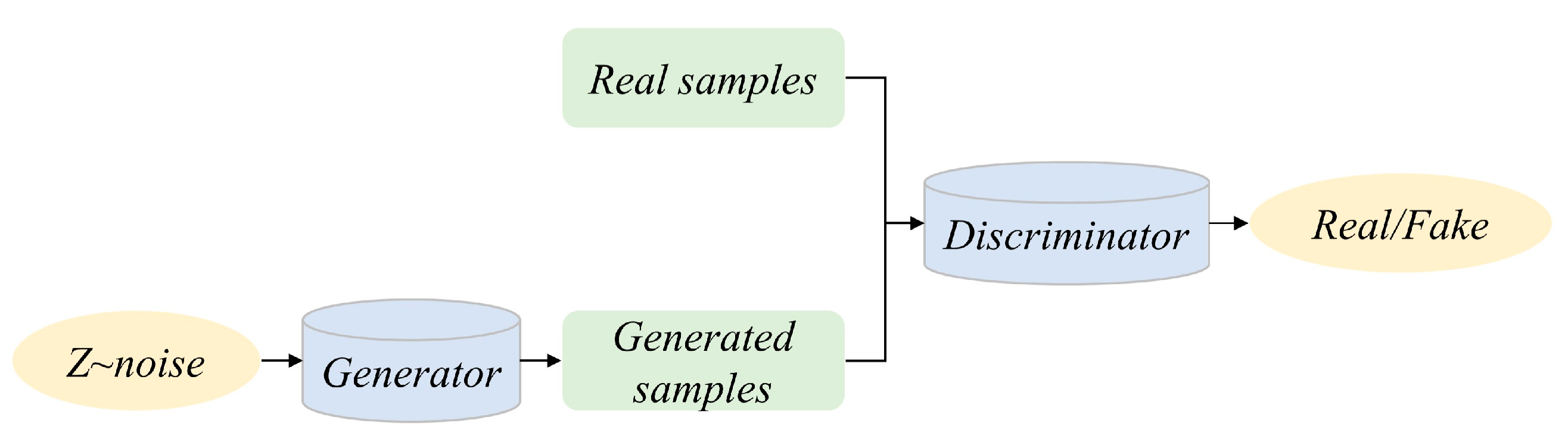
GAN is an unsupervised generative model proposed by Goodfellow et al. in 2014, which is created based on zero-sum game theory and mainly consists of a generator G and a discriminator D [20]. The architecture of a basic GAN is shown in Figure 1. The generator obtains the generative sample G(z) from random noise z, and the discriminator is used to discriminate whether the input sample is a real sample x or a generative sample G(z). Through iterative adversarial training, the performance of the generator and the discriminator are simultaneously improved, eventually reaching Nash equilibrium. The loss function of GAN is defined as:
where Pr(x) and Pz(z) are the prior distributions of x and z, respectively, Ex~Pr(x) denotes the expectation of x from Pr(x), Ez~Pz(z) denotes the expectation of z from Pz(z). The generator’s goal is to minimize V(D,G), while the discriminator’s goal is to maximize V(D,G) in the adversarial training process.
2.2. SGAN
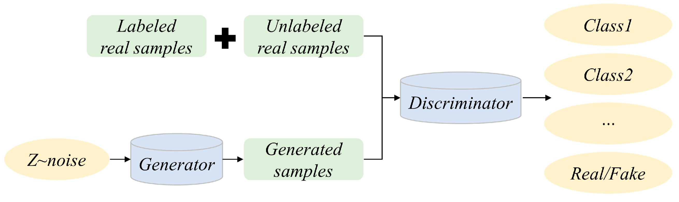
SGAN is a semi-supervised generative model that Augustus Odena et al. proposed in 2016. SGAN extends GAN to semi-supervised scenarios by forcing the discriminator to output category labels [21]. The discriminator of traditional GAN uses a Sigmoid function as the output, while SGAN uses a Softmax function as the output. For a dataset with N categories, the discriminator extends the output to N + 1, including one discriminative output and N categorical output. The architecture of a basic SGAN is shown in Figure 2, and the input of the discriminator consists of three parts: labeled real samples, unlabeled real samples, and generated samples from the generator. The loss function of SGAN is defined as:
where Lg and Ld represent the loss functions of the generator and the discriminator, respectively. Lsupervise and Lunsupervised denote the discriminator’s supervised loss function and the unsupervised loss function, respectively.
2.3. ACGAN
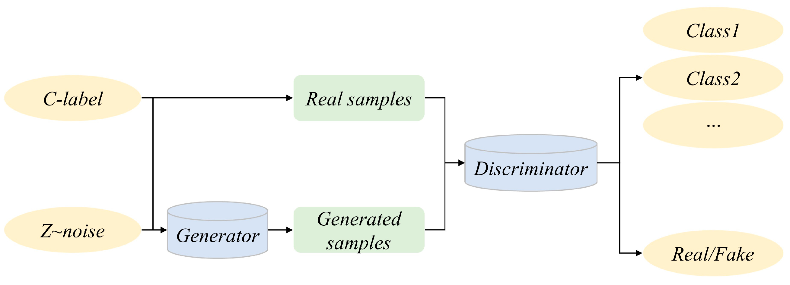
ACGAN is a supervised generative model that Augustus Odena et al. proposed in 2017 [22]. The architecture of the basic ACGAN is shown in Figure 3. By embedding the category labels as auxiliary information into the random noise input, the generator is guided to generate multi-mode samples. Unlike SGAN, the discriminator of ACGAN uses a Sigmoid function and a Softmax function as outputs to achieve discrimination and classification of the input samples. The loss function of ACGAN consists of two components:
where Lsource denotes the loss function used to measure the validity of discriminating samples from x, Lclass denotes the loss function used to measure the validity of sample categories, and cr and cg are labels of x and G(z,cg), respectively. P(c = cr|x) and P(c = cg|G(z,cg)) are the conditional probability distributions of class labels x and G(z,cg), respectively. During adversarial training, the discriminator is trained to maximize Lclass + Lsource, while the generator’s goal is to maximize Lclass − Lsource.
3. The Proposed SACGAN
SACGAN combines the respective features of SGAN and ACGAN and utilizes the semi-supervised learning mechanism of SGAN to improve generation, discrimination, and classification abilities by adversarial training using labeled and unlabeled data, thus transforming ACGAN from supervised learning to semi-supervised learning.
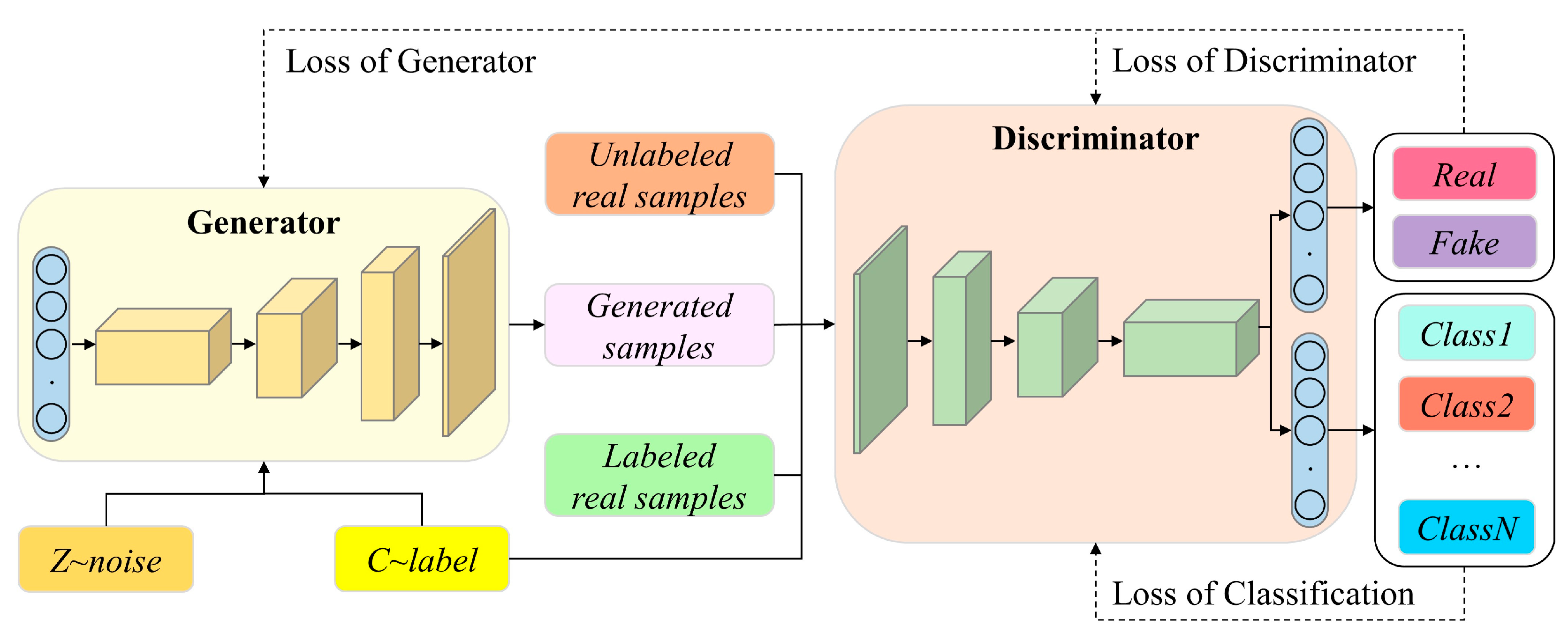
3.1. Architecture of SACGAN
SACGAN refers to the structure of a Deep Convolutional Generative Adversarial Network (DCGAN) [23]. It is designed based on convolutional and deconvolutional networks; the architecture of SACGAN is shown in Figure 4. The generator mainly consists of embedding layers and two-dimensional deconvolutional layers; the input is a random noise vector with a category label vector, and the output is generated samples. The discriminator mainly consists of two-dimensional convolutional layers and fully connected layers, and the input includes labeled real samples, unlabeled real samples, and generated samples from the generator, and the output comprises discrimination results and classification results.
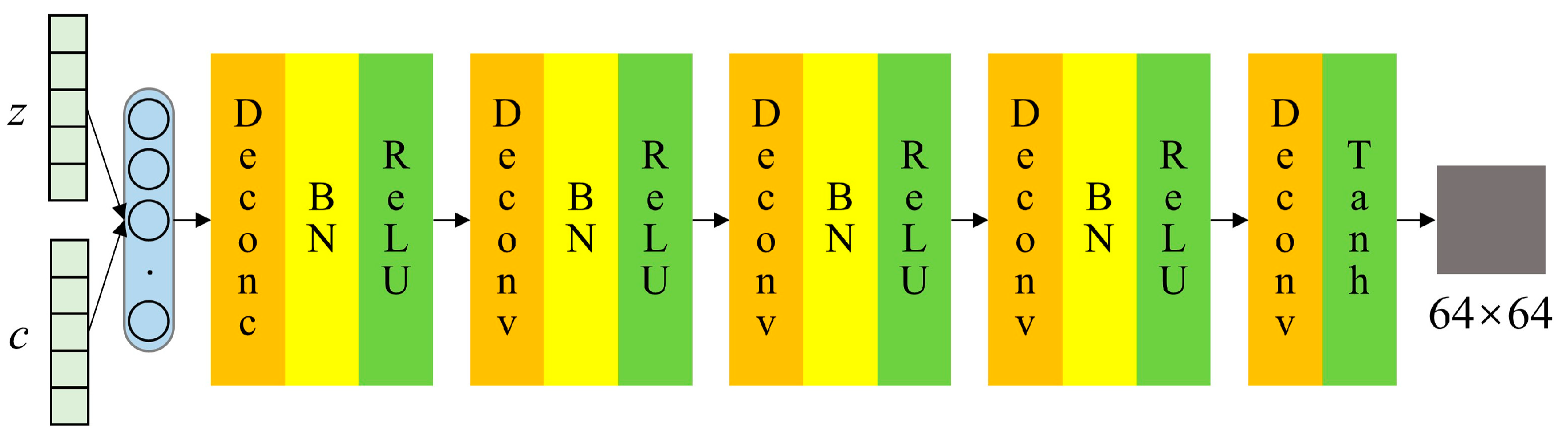
3.2. Structure of Generator
The generator’s input is a 200-dimensional Gaussian random noise vector z with a label vector c. The label vector is first embedded in the noise vector through an embedding layer, followed by deconvolution layers to generate fake samples whose sizes are 64 × 64. The generator contains five deconvolution layers, and the activation function of the first four layers is ReLU, which helps the generator achieve non-linear representations and makes the network easier for training. The activation function of the last layer is Tanh, which limits the output to [−1,1], and BN is executed after each layer to speed up the training convergence and avoid overfitting. The specific structure is shown in Figure 5, and the detailed parameters are shown in Table 1.
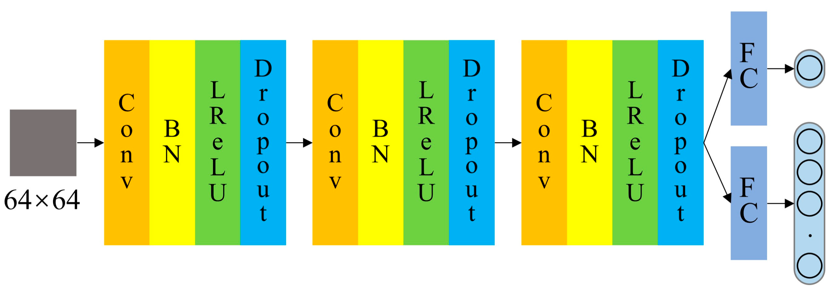
3.3. Structure of the Discriminator
The input of the discriminator is real samples and generated samples, and the output is a discrimination vector with a classification vector. The discriminator contains three convolutional layers, each with a leaky ReLU activation function, which allows the network to learn faster and prevent gradient disappearance. After each convolution, BN is executed first, followed by Dropout, which randomly drops neurons in the network to reduce the risk of overfitting and thus increase the generalization of the discriminator. The last layer contains two fully connected layers, using a Sigmoid function and a Softmax function as outputs for discriminating and classifying the input samples. The specific structure is shown in Figure 6, and the detailed parameters are shown in Table 2.
3.4. Loss Functions of SACGAN
SACGAN is constructed based on SGAN and ACGAN, so the loss functions of SACGAN combine the loss functions of SGAN and ACGAN. More specifically, the loss function of the generator of SACGAN is the same as that of ACGAN, and the loss function of the discriminator is referenced from SGAN, which consists of the supervised loss function of labeled data and the unsupervised loss function of unlabeled data. The specific definitions are as follows:
where LG and LD represent the loss functions of the generator and the discriminator, respectively; and represent the supervised loss and the unsupervised loss of the discriminator, and , are the ratio factors; Pr(x) and Pr(x,y) are the prior distributions of labeled real samples and unlabeled real samples, respectively; c are labels of labeled real samples; and P(c = c|x) and P(c = c|G(z,c)) are the conditional probability distributions of class labels of labeled real samples and generated samples, respectively.
4. Fault Diagnosis Based on STFT-SACGAN
4.1. Data Processing
STFT is a joint time-varying time-frequency analysis method for non-stationary signals that converts one-dimensional time-domain signals into two-dimensional time-frequency images for CNN processing: feature spectra containing both time-domain and frequency-domain information. It uses a fixed-length window function to translate over the time-domain signal, intercepting it and performing a Fourier transform to obtain a local set of spectra for each period [24]. Therefore, STFT is a 2D function of time and frequency, whose calculation formula is defined as:
where x(t) represents the one-dimensional time-domain signal, t and w are the time and the frequency, respectively, and g(t − τ) denotes a window function whose center is at the time τ.
The time and frequency resolutions of the spectrum obtained by STFT depend on the length of the window function, with longer window lengths yielding a lower time resolution and a higher frequency resolution. Therefore, the window length should be chosen reasonably according to the signal to be processed for better analysis [25]. The time and frequency resolutions are calculated as follows:
where Nx is the length of the signal to be processed, Nw is the length of the window function, No is the overlapped length during the translation of the window function, and [·] represents the operation of rounding down.
This paper converts the original one-dimensional vibration signals of bearings into two-dimensional time-frequency images by STFT, which carry richer information and characterize a more complex structural distribution. According to Equations (13) and (14), the time-frequency image after STFT is a two-dimensional matrix of dimension F × T. Let X denote the obtained matrix, and to speed up the convergence of the training process, each element of the matrix X is normalized into the interval [−1,1] according to Equation (16).
4.2. Fault Diagnosis Flow Based on STFT-SACGAN
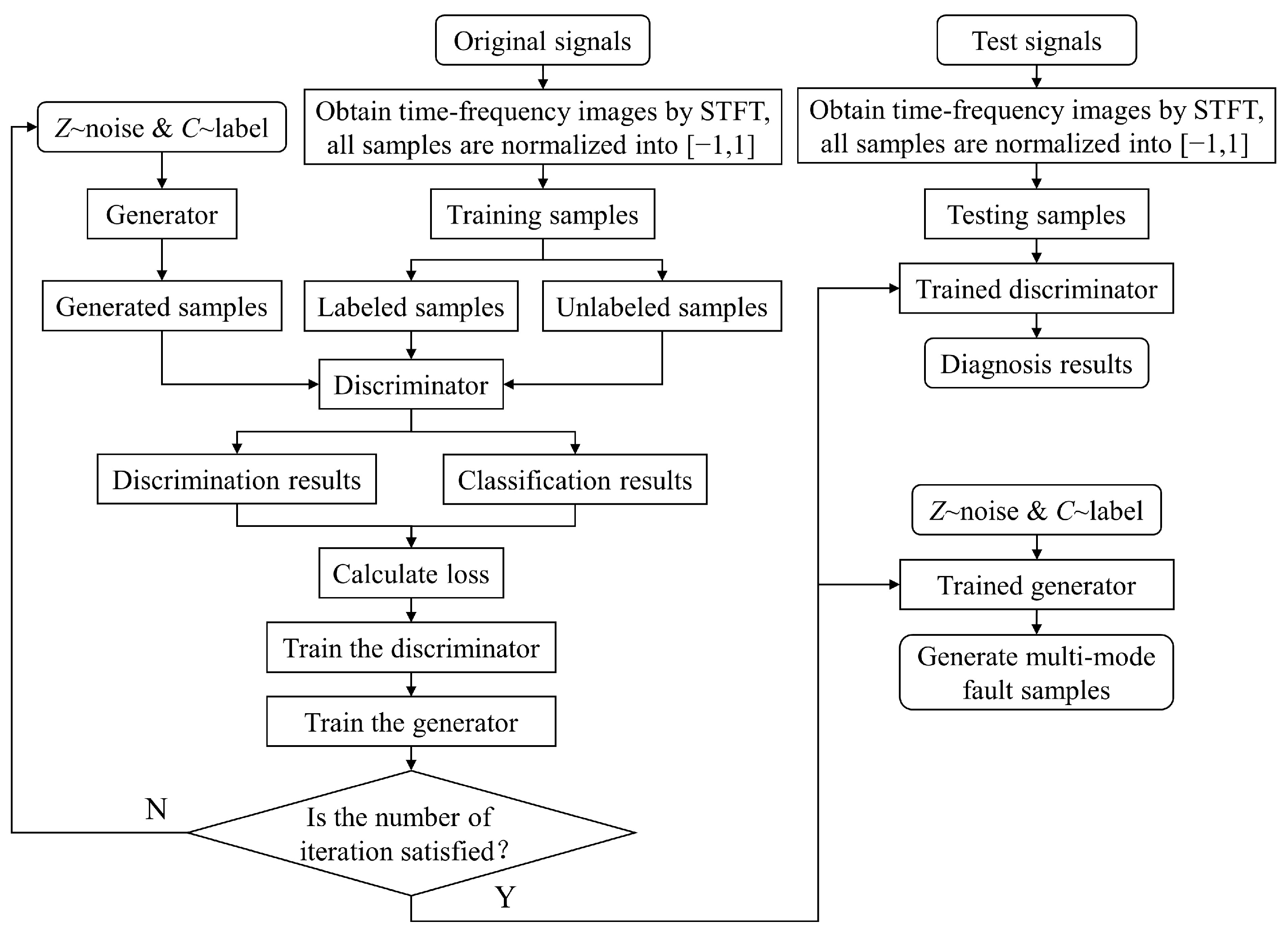
A fault diagnosis method based on STFT-SACGAN is proposed, using the ability of STFT to process non-stationary signals. The original one-dimensional vibration signals of bearings are converted into two-dimensional time-frequency images by STFT as the input of SACGAN. The multi-mode fault sample generation ability of the generator and the recognition ability of the discriminator are improved by adversarial training. The flow of the proposed method is shown in Figure 7, and the main steps are as follows:
- (1)
- Vibration signals of bearings with various fault modes are collected, converted into time-frequency images by STFT, and normalized into the interval [−1,1];
- (2)
- The noise vector z and the label vector c are input to the generator to obtain generated samples;
- (3)
- Labeled real samples, unlabeled real samples, and generated samples from the generator are fed into the discriminator to obtain discrimination and classification results.
- (4)
- Calculate the loss of the generator and the discriminator;
- (5)
- Fix the generator’s weight parameters and optimize the discriminator’s weight parameters;
- (6)
- Fix the discriminator’s weight parameters and optimize the generator’s weight parameters;
- (7)
- Repeat steps 2–6 until the number of iterations is satisfied;
- (8)
- Save the trained model, use the generator to generate multi-mode fault samples, and use the discriminator for fault diagnosis of test signals.
5. Case Study
To demonstrate the effectiveness and generalization of the proposed method, validation and analysis are carried out on two bearing datasets. In those two case studies, the computer is a Core i5-9300H CPU @ 2.40 GHz with 16 GB of Ram and works in the Windows 64-bit operating system, and a GPU(GTX1650) with 4 GB of memory is added to improve the training speed. The programming language is Python 3.8.13, and the deep learning framework is Pytorch 1.10.1. During the training process, the generator and the discriminator of SACGAN use the Adam optimization algorithm [26], and the learning rate is 0.0005. To reduce the fluctuation during training, the exponential decay rates β1 and β2 are set to 0.5 and 0.999, respectively [27]. The batch size is K × 10 (K is the number of category labels), the dropout rate of the discriminator is 0.25, and the number of iterations is 200. In addition, the ratio factors of the loss function Equation (11) are set to 0.5 and 0.5, respectively.
5.1. Case 1 Multi-Mode Data Generation and Fault Diagnosis of Bearings
5.1.1. Introduction and Preprocessing of Bearing Data
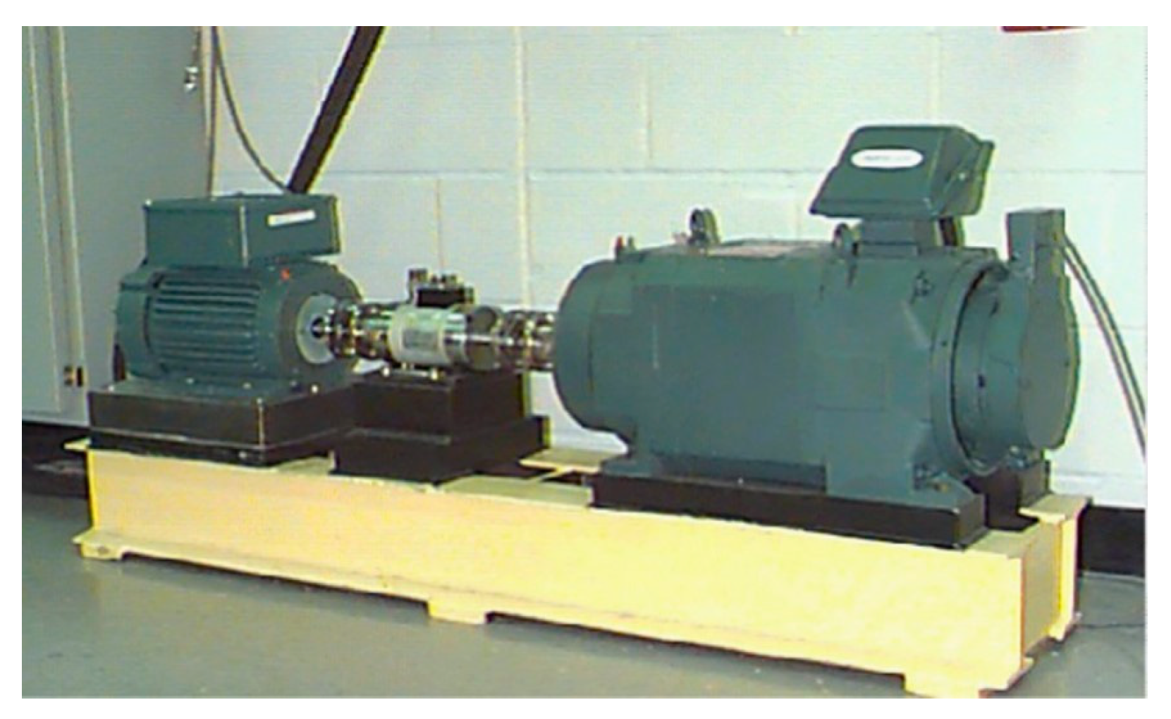
In case 1, the Case Western Reserve University (CWRU)-bearing dataset is used to verify the effectiveness of the proposed method, and the test rig is shown in Figure 8 [28]. Specifically, ten kinds of bearing vibration data under 1797 rpm and 12 kHz sampling frequency are used for analysis. Bearing states include one normal state and nine faulty states, including three fault locations and three fault sizes, as listed in Table 3. The vibration signals from each state are randomly sampled 300 times over 1024 points as available samples, of which 100 samples from each state are used as testing samples. The remaining samples are divided into labeled and unlabeled training samples according to different ratios.
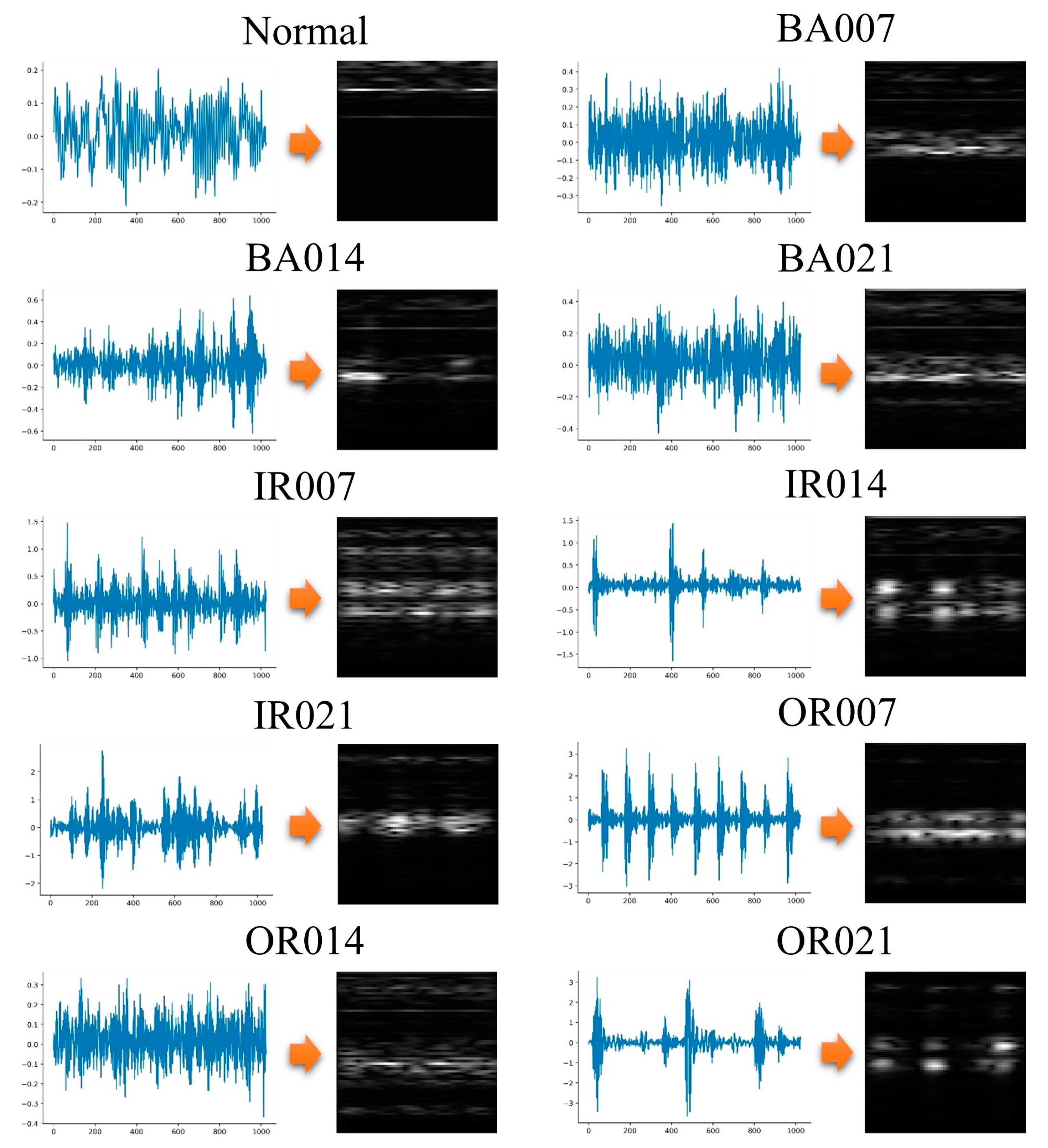
All samples are converted into time-frequency images by STFT. According to Section 3.1, the window function is Hanning window; the window function length Nw and the overlap length No are set to 256 and 250, respectively. The normalized time-frequency matrix is geometrically processed into a 64 × 64 square matrix as the input of SACGAN to accommodate the training of SACGAN and save computation time. The original time-domain vibration signals and the corresponding two-dimensional time-frequency images obtained by conversion are shown in Figure 9. It can be seen that characteristic differences between different states are more significant than the original one-dimensional time-domain vibration signals after conversion.
5.1.2. Quality Evaluation and Comparison of Multi-Mode Generated Samples
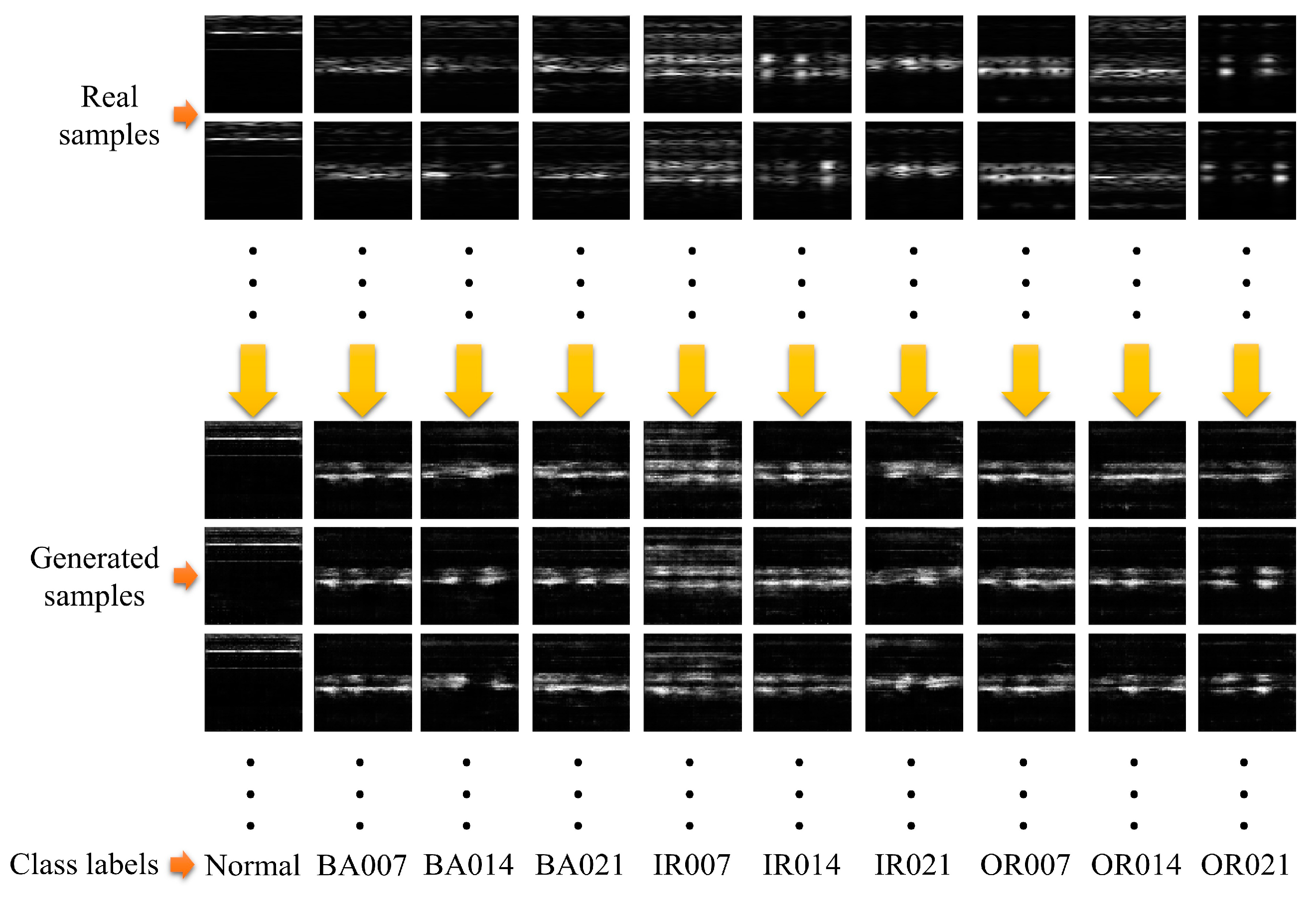
The sample generation ability of the generator is usually verified by evaluating the quality of the generated samples. In this case study, the SAGAN is trained using training samples with a labeling ratio of 0.2 (40 labeled samples and 160 unlabeled samples of each class). The diagrammatic sketch of the real samples and the generated samples is shown in Figure 10. The generated multi-mode samples are highly similar to the real samples.
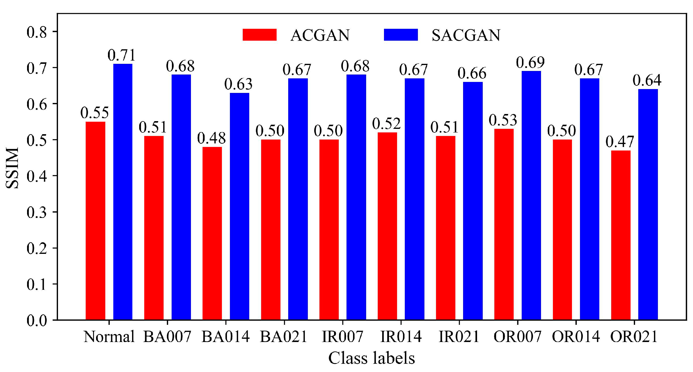
For a more objective evaluation, the structural similarity index measure (SSIM) is used to quantitatively evaluate the quality of the generated multi-mode samples. The SSIM aims to measure the similarity of two images from brightness, contrast, and structure. The range of SSIM values is the interval [−1,1], and larger SSIM values indicate higher similarity between two images [29]. In contrast, the labeled training samples are also used to train the ACGAN, where the parameter structure of the ACGAN is the same as that of the SACGAN. Five pairs of the real samples and the generated samples of each class are randomly selected, and the average SSIM values of the ACGAN and the SACGAN are given in Figure 11. The results show that the average SSIM values of each class of the SACGAN are always larger than those of the ACGAN, meaning that the samples generated by the SACGAN are closer to the real samples.
5.1.3. Fault Recognition with Different Label Ratios
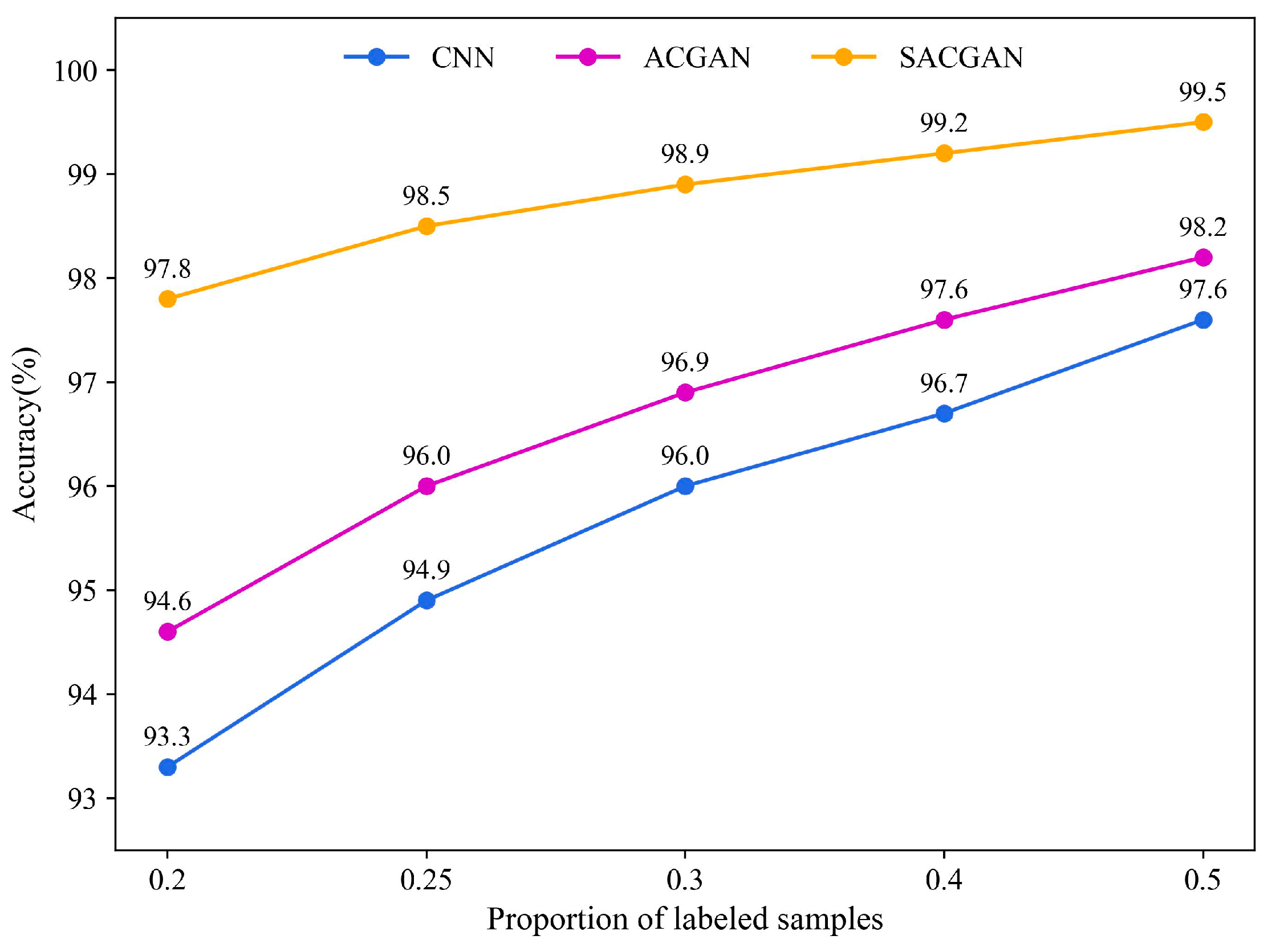
Each class’s training samples are divided into labeled and unlabeled samples in different ratios to train the SACGAN. The labeled samples are also used to train the ACGAN and the CNN model for comparison, where the parameter structure of the ACGAN is the same as the SACGAN. It is worth mentioning that to verify the effectiveness of the discriminator’s structure, the CNN model here is the discriminator of SACGAN that can perform supervised learning. Each group of comparative experiments is repeated ten times, and the average recognition accuracy of the test samples at different label ratios is given in Figure 12. The results show that all three models have high recognition accuracy, indicating the effectiveness of the discriminator structure; the ACGAN and the SACGAN effectively improve the recognition ability of the discriminator through adversarial learning; limiting the number of labeled training samples has a greater impact on the fault recognition ability of the ACGAN and the CNN and the SACGAN can weaken the influence of decreasing labeled training samples and has the highest recognition accuracy under different label ratios.
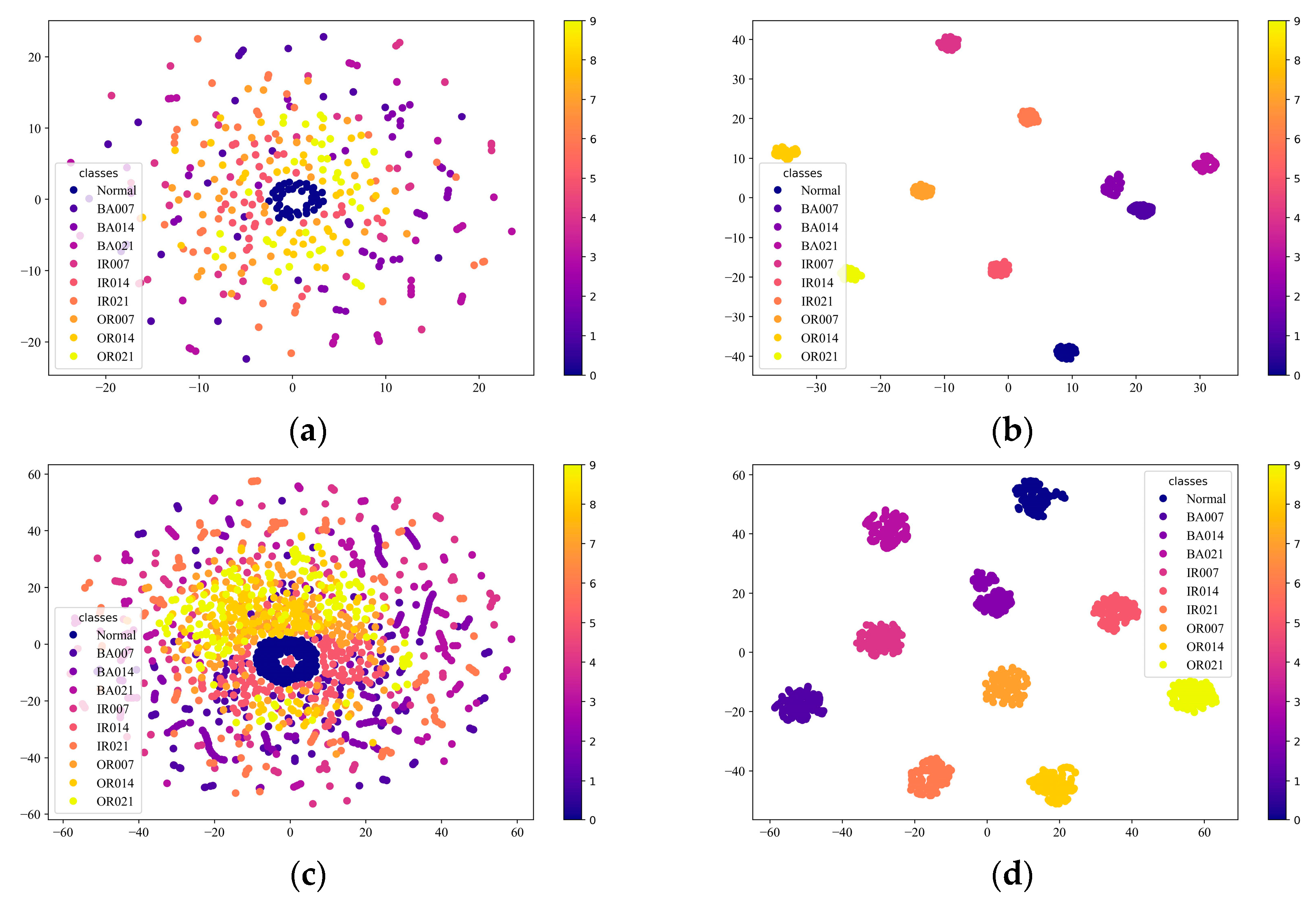
The recognition ability of the model is closely related to its ability to extract effective features, and to observe the distribution of features extracted by the model, the t-SNE (t-Distributed Stochastic Neighbor Embedding) algorithm is used to visualize the distribution of extracted features [30]. The changes in the distribution of labeled training and testing samples with a labeling ratio of 0.2 are shown in Figure 13, which shows that the SACGAN can significantly improve the distribution of samples from a different class, reduce the intra-class distance, and increase the inter-class distance, making it easier to recognize the differences between different classes.
5.2. Case 2 Multi-Mode Data Generation and Fault Diagnosis of Bearings
5.2.1. Introduction and Preprocessing of Bearing Data
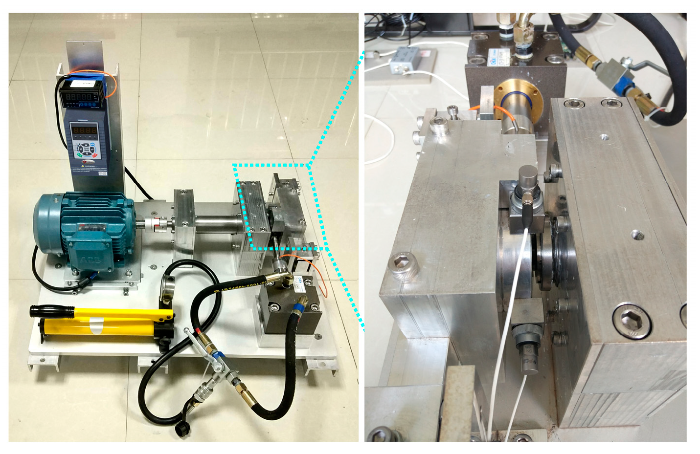
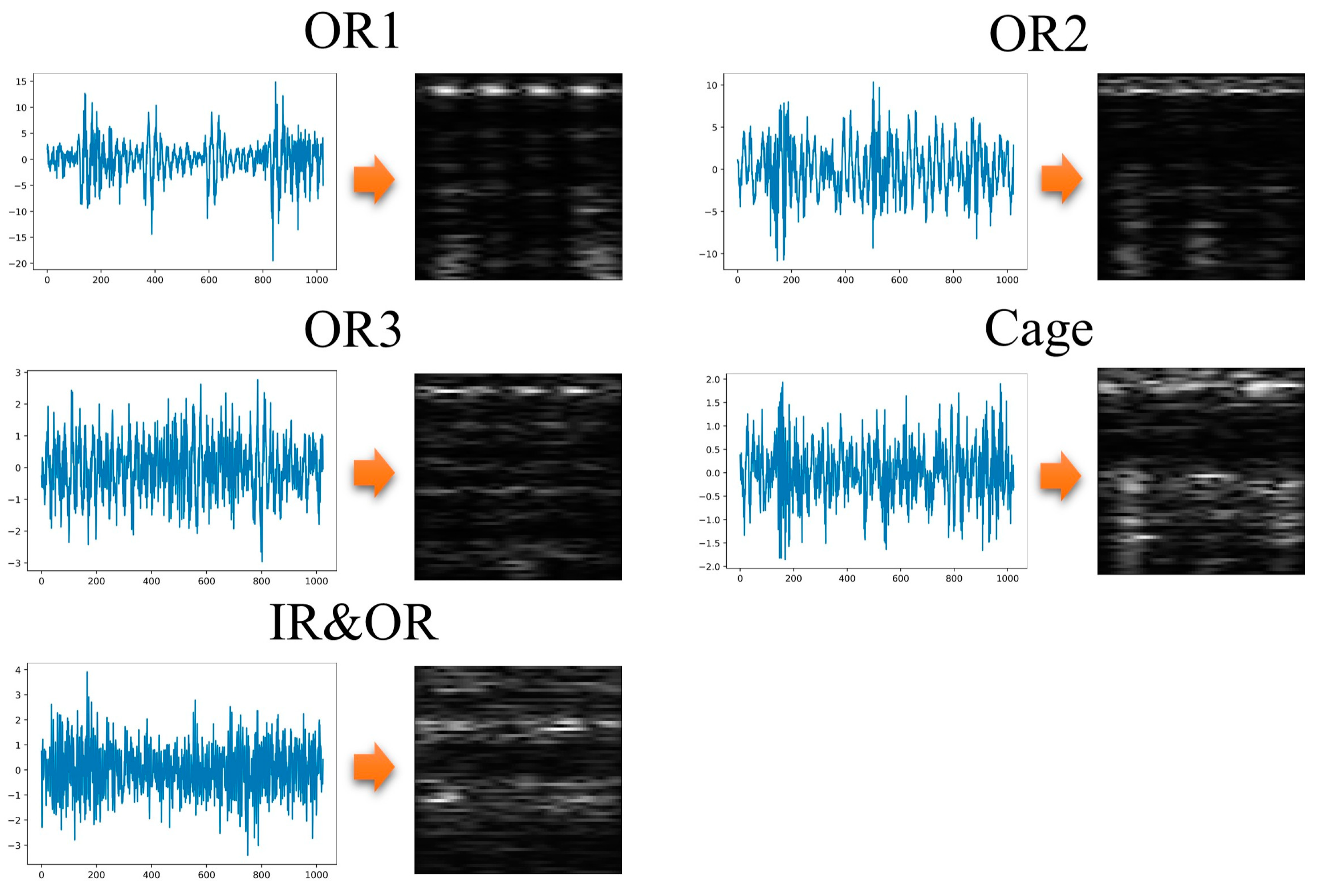
In case 2, Xi’an Jiaotong University and the Changxing Sumyoung Technology Co. (XJTU-SY) bearing dataset are used to verify the generalization ability of the proposed method, and the test rig is shown in Figure 14 [31], with a sampling frequency of 2.56 kHz. Five kinds of bearing vibration data with a speed of 2100 rpm and a radial force of 12 kN are selected for analysis, and the bearing states and class labels are shown in Table 4. Similar to Case 1, 1024 consecutive points are randomly sampled 300 times from the vibration signals of each state as available samples, and two-dimensional time-frequency images obtained by conversion are shown in Figure 15.
5.2.2. Multi-Mode Fault Sample Generation and Fault Recognition in Case 2
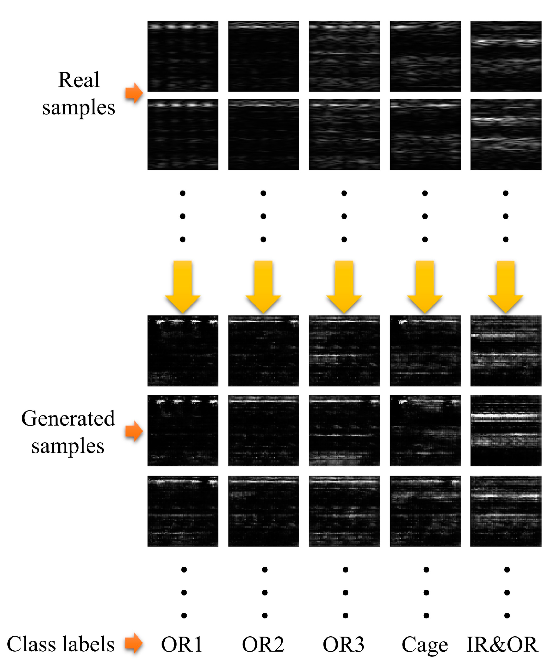
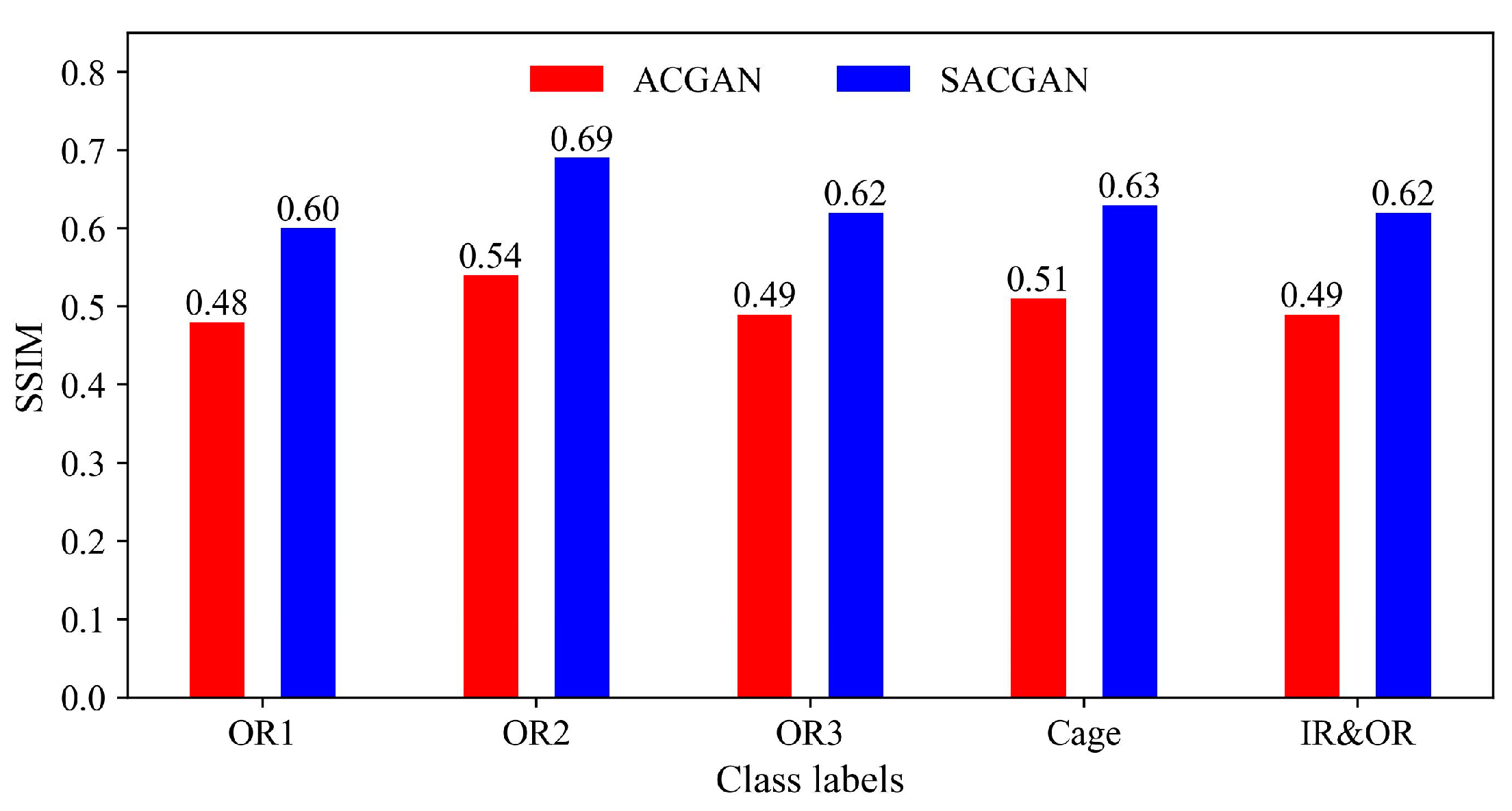
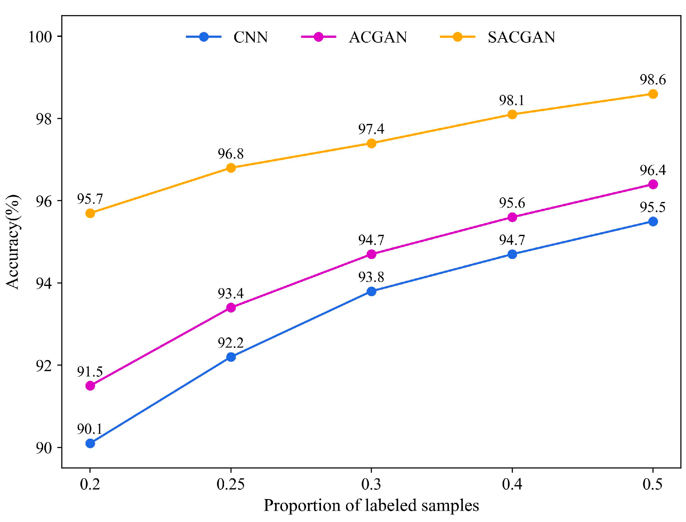
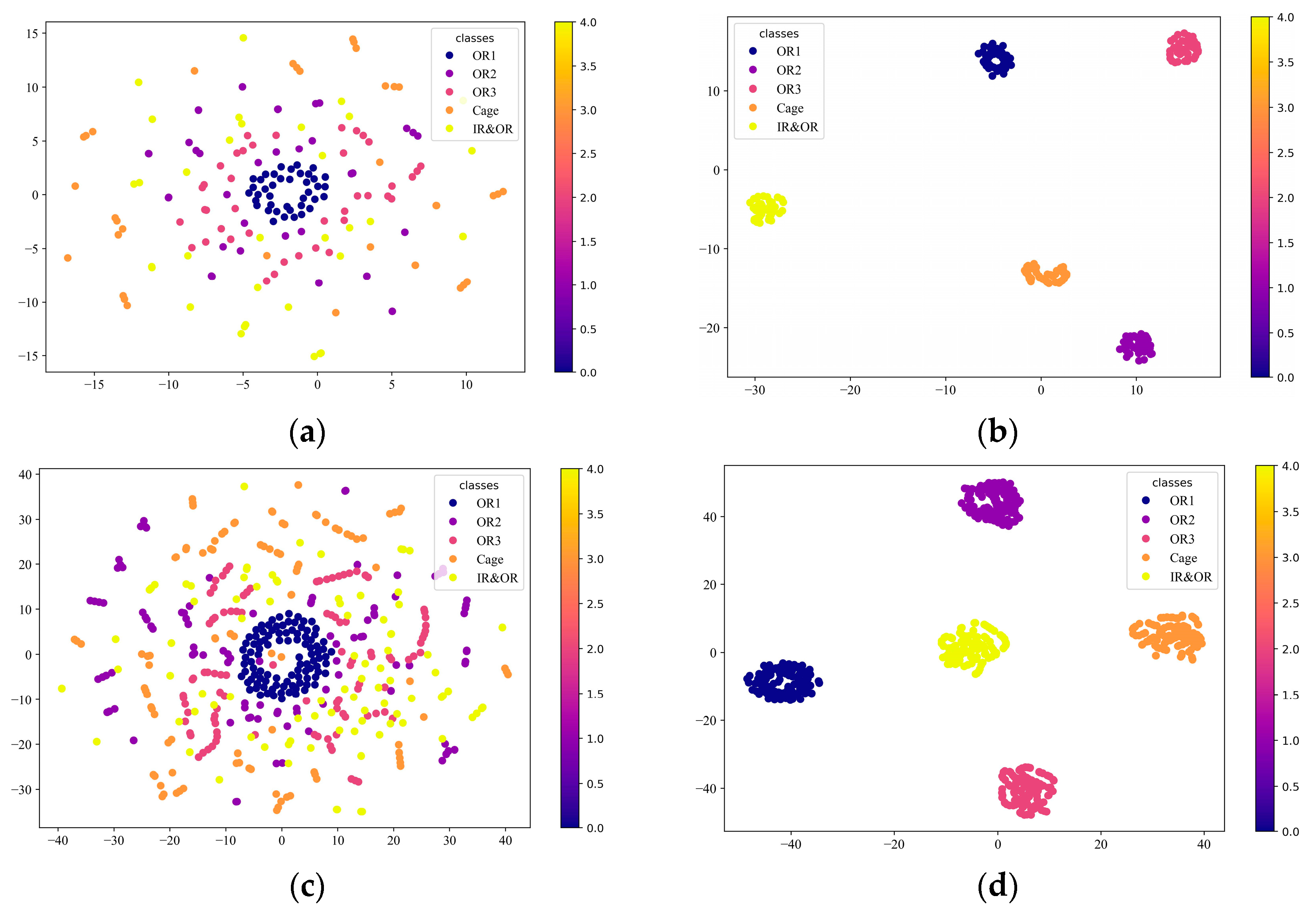
Similar to Case 1, the SAGAN is trained using training samples with a labeling ratio of 0.2 (40 labeled samples and 160 unlabeled samples of each class). Figure 16 shows the diagrammatic sketch of the real samples and the generated samples. The SSIM is also used to quantitatively evaluate the quality of the generated multi-mode samples. As shown in Figure 17, the SSIM values of each class of the ACGAN are always smaller than those of the SACGAN. The results further demonstrate the validity and superiority of the SACGAN in terms of generation. The comparative fault recognition experiments are the same as in Case 1, and the recognition accuracies of the test samples at different label ratios are shown in Figure 18. For feature-level evaluation, the results of feature distribution visualization are shown in Figure 19. The above results proved that the SACGAN has strong robustness and generalization ability and can be applied to different objects and operating environments.
6. Conclusions
To address the problem of scarcity of labeled data in intelligent fault diagnosis of bearings, from the field of GAN, the SACGAN based on SGAN and ACGAN is constructed to improve the multi-mode fault sample generation ability of the generator and the recognition ability of the discriminator by using a small amount of labeled data with a large amount of unlabeled data for adversarial learning. Using the ability of STFT to process non-stationary signals, a fault diagnosis method based on STFT-SACGAN is proposed, and the original one-dimensional vibration signals of bearings are converted into two-dimensional time-frequency images by STFT as the input of the SACGAN. The effectiveness of the proposed method is verified on the CWRU bearing dataset, and the results show that the SACGAN can generate high-quality multi-mode fault samples and has excellent fault recognition ability. The proposed method is verified to have strong generalization and stability on the XJTU-SY bearing dataset.
Although the proposed method can perform multi-mode fault sample generation and fault diagnosis tasks well, it only involves data from a single source of information. In the future, we will explore how to use data from multi-source information fusion to generate high-quality, multi-source information fusion fault samples and further optimize the model to improve fault diagnosis efficiency. In addition, the study of fault diagnosis with limited labeled data is more suitable to current industrial practical scenarios. It can significantly reduce the cost of fault diagnosis, which is worth further exploration.
Author Contributions
Conceptualization, H.W.; methodology, H.W.; software, H.W.; validation, H.W.; formal analysis, H.W.; investigation, H.W.; data curation, H.W.; writing—original draft preparation, H.W.; writing—review and editing, H.W.; visualization, H.W.; supervision, H.Z. and H.L.; project administration, H.Z.; funding acquisition, H.Z. All authors have read and agreed to the published version of the manuscript.
Funding
This work was supported by the National Natural Science Foundation of China (Grant No. 52277055).
Data Availability Statement
The data used to support this study are available on the websites https://engineering.case.edu/bearingdatacenter/download-data-file and https://biaowang.tech/xjtu-sy-bearing-datasets/, accessed on 22 March 2023.
Conflicts of Interest
The authors declare no conflict of interest.
References
- Lei, Y.G.; Yang, B.; Jiang, X.W.; Jia, F.; Li, N.P.; Nandi, A. Applications of machine learning to machine fault diagnosis: A review and roadmap. Mech. Syst. Signal Process. 2020, 138, 106587–106625. [Google Scholar] [CrossRef]
- Sun, Y.J.; Wang, J.; Wang, X.H. Fault diagnosis of mechanical equipment in high energy consumption industries in China: A review. Mech. Syst. Signal Process. 2023, 186, 109833–109865. [Google Scholar] [CrossRef]
- Zhao, Z.B.; Li, T.F.; Wu, J.Y.; Sun, C.; Wang, S.B.; Yan, R.Q.; Chen, X.F. Deep learning algorithms for rotating machinery intelligent diagnosis: An open source benchmark study. ISA Trans. 2020, 107, 224–255. [Google Scholar] [CrossRef] [PubMed]
- Cen, J.; Yang, Z.H.; Liu, X.; Xiong, J.B.; Chen, H.H. A Review of Data-Driven Machinery Fault Diagnosis Using Machine Learning Algorithms. J. Vib. Eng. Technol. 2022, 10, 2481–2507. [Google Scholar] [CrossRef]
- Jalayer, M.; Orsenigo, C.; Vercellis, C. Fault detection and diagnosis for rotating machinery: A model based on convolutional LSTM, Fast Fourier and continuous wavelet transforms. Comput. Ind. 2021, 125, 103378–103393. [Google Scholar] [CrossRef]
- Przystupa, K.; Ambrożkiewicz, B.; Litak, G. Diagnostics of Transient States in Hydraulic Pump System with Short Time Fourier Transform. Adv. Sci. Technol. Res. J. 2020, 14, 178–183. [Google Scholar] [CrossRef]
- Lepicka, M.; Górski, G.; Gradzka-Dahlke, M.; Litak, G.; Ambrożkiewicz, B. Analysis of tribological behaviour of titanium nitride-coated stainless steel with the use of wavelet-based methods. Arch. Appl. Mech. 2021, 91, 4475–4483. [Google Scholar] [CrossRef]
- Kibrete, F.; Woldmichael, D.E. Applications of Artificial Intelligence for Fault Diagnosis of Rotating Machines: A Review. Inst. Comput. Sci. Soc. Inform. Telecommun. Eng. 2023, 455, 41–62. [Google Scholar]
- Zhu, Z.Q.; Lei, Y.B.; Qi, G.Q.; Chai, Y.; Mazur, N.; An, Y.; Huang, X.H. A review of the application of deep learning in intelligent fault diagnosis of rotating machinery. Measurement 2023, 206, 112346–112369. [Google Scholar] [CrossRef]
- Zhao, Z.B.; Wu, J.Y.; Li, T.F.; Sun, C.; Yan, R.Q.; Chen, X.F. Challenges and Opportunities of AI-Enabled Monitoring, Diagnosis & Prognosis: A Review. Chin. J. Mech. Eng. 2021, 34, 16–44. [Google Scholar]
- Zhang, T.C.; Chen, J.L.; Li, F.D.; Zhang, K.Y.; Lv, H.X.; He, S.L.; Xu, E.Y. Intelligent fault diagnosis of machines with small & imbalanced data: A state-of-the-art review and possible extensions. ISA Trans. 2021, 119, 152–171. [Google Scholar] [PubMed]
- Zhao, Z.B.; Zhang, Q.Y.; Yu, X.L.; Sun, C.; Wang, S.B.; Yan, R.Q.; Chen, X.F. Applications of Unsupervised Deep Transfer Learning to Intelligent Fault Diagnosis: A Survey and Comparative Study. IEEE Trans. Instrum. Meas. 2021, 70, 3525828–3525855. [Google Scholar] [CrossRef]
- Pan, T.Y.; Chen, J.L.; Zhang, T.C.; Liu, S.; He, S.L.; Lv, H.X. Generative adversarial network in mechanical fault diagnosis under small sample: A systematic review on applications and future perspectives. ISA Trans. 2021, 128, 1–10. [Google Scholar] [CrossRef] [PubMed]
- Pang, X.Y.; Wei, Z.H.; Tong, Y. Fault Diagnosis Method of Gear Based on SCGAN Network. J. Vib. Meas. Diagn. 2022, 42, 358–364. [Google Scholar]
- Xing, X.S.; Guo, W. Intelligent diagnosis method for bearing with few labelled samples based on an improved semi-supervised learning-based generative adversarial network. J. Vib. Shock 2022, 41, 184–192. [Google Scholar]
- Yang, Q.; Zhang, J.Y.; Wu, D.S.; Liu, Y.P. Fault Diagnosis for Rolling Bearings Based on Two-Dimensional Image and Switchable Normalization SGAN Network. Bearing 2021, 8, 39–46. [Google Scholar]
- Lu, J.L.; Zhang, X.G.; Zhang, W.; Guo, L.Y.; Wen, R.T. Fault Diagnosis of Main Bearing of Wind Turbine Based on Improved Auxiliary Classifier Generative Adversarial Network. Autom. Electr. Power Syst. 2021, 45, 148–154. [Google Scholar]
- Li, D.D.; Liu, Y.H.; Zhao, Y.; Zhao, Y. Fault Diagnosis Method of Wind Turbine Planetary Gearbox Based on Improved Generative Adversarial Network. Proc. CSEE 2021, 41, 7496–7507. [Google Scholar]
- Li, W.; Zhong, X.; Shao, H.D.; Cai, B.P.; Yang, X.K. Multi-mode data augmentation and fault diagnosis of rotating machinery using modified ACGAN designed with new framework. Adv. Eng. Inform. 2022, 52, 101552–101567. [Google Scholar] [CrossRef]
- He, W.P.; Chen, J.; Zhou, Y.; Liu, X.; Chen, B.Q.; Guo, B.L. An Intelligent Machinery Fault Diagnosis Method Based on GAN and Transfer Learning under Variable Working Conditions. Sensors 2022, 22, 9175. [Google Scholar] [CrossRef]
- He, Y.; Tang, H.S.; Ren, Y.; Kumar, A. A semi-supervised fault diagnosis method for axial piston pump bearings based on DCGAN. Meas. Sci. Technol. 2021, 32, 125104–125122. [Google Scholar] [CrossRef]
- Meng, Z.; Li, Q.; Sun, D.Y.; Cao, W.; Fan, F.J. An Intelligent Fault Diagnosis Method of Small Sample Bearing Based on Improved Auxiliary Classification Generative Adversarial Network. IEEE Sens. J. 2022, 22, 19543–19555. [Google Scholar] [CrossRef]
- Gao, Y.D.; Piltan, F.; Kim, J.M. A Novel Image-Based Diagnosis Method Using Improved DCGAN for Rotating Machinery. Sensors 2022, 22, 7534. [Google Scholar] [CrossRef] [PubMed]
- Li, H.; Zhang, Q.; Qin, X.R.; Sun, Y.T. Fault diagnosis method for rolling bearings based on short-time Fourier transform and convolution neural network. J. Vib. Shock 2018, 37, 124–131. [Google Scholar]
- Tao, H.F.; Wang, P.; Chen, Y.Y.; Stojanovic, V.; Yang, H.Z. An unsupervised fault diagnosis method for rolling bearing using STFT and generative neural networks. J. Frankl. Inst. 2020, 357, 7286–7307. [Google Scholar] [CrossRef]
- Kingma, D.P.; Ba, J. Adam: A Method for Stochastic Optimization. arXiv 2014, arXiv:1412.6980. [Google Scholar]
- Radford, A.; Metz, L.; Chintala, S. Unsupervised Representation Learning with Deep Convolutional Generative Adversarial Networks. arXiv 2015, arXiv:1511.06434. [Google Scholar]
- Smith, W.; Randall, R. Rolling element bearing diagnostics using the Case Western Reserve University data: A benchmark study. Mech. Syst. Signal Process. 2015, 64–65, 100–131. [Google Scholar] [CrossRef]
- Setiadi, D. PSNR vs. SSIM: Imperceptibility quality assessment for image steganography. Multimed. Tools Appl. 2021, 80, 8423–8444. [Google Scholar] [CrossRef]
- Pezzotti, N.; Lelieveldt, B.; Maaten, L.; Höllt, T.; Eisemann, E.; Vilanova, A. Approximated and User Steerable tSNE for Progressive Visual Analytics. IEEE Trans. Vis. Comput. Graph. 2017, 23, 1739–1752. [Google Scholar] [CrossRef]
- Wang, B.; Lei, Y.G.; Li, N.P.; Li, N.B. A Hybrid Prognostics Approach for Estimating Remaining Useful Life of Rolling Element Bearings. IEEE Trans. Reliab. 2020, 69, 401–412. [Google Scholar] [CrossRef]
Figure 1.
Architecture of GAN.

Figure 2.
Architecture of SGAN.

Figure 3.
Architecture of ACGAN.

Figure 4.
Architecture of SACGAN.

Figure 5.
Structure of the generator.

Figure 6.
Structure of the discriminator.

Figure 7.
Fault diagnosis flowchart based on STFT-SACGAN.

Figure 8.
CWRU-bearing experimental platform.

Figure 9.
Time-domain vibration signals for CWRU data and the corresponding time-frequency images obtained by conversion.
Figure 9.
Time-domain vibration signals for CWRU data and the corresponding time-frequency images obtained by conversion.

Figure 10.
The diagrammatic sketch of generating samples for CWRU data.

Figure 11.
Quality evaluation of generated samples based on the SSIM for CWRU data.

Figure 12.
Recognition results with different label ratios for CWRU data.

Figure 13.
Visualization of feature distribution for CWRU data. (a) Labeled samples before training; (b) labeled samples after training; (c) test samples before testing; (d) test samples after testing.
Figure 13.
Visualization of feature distribution for CWRU data. (a) Labeled samples before training; (b) labeled samples after training; (c) test samples before testing; (d) test samples after testing.

Figure 14.
XJTU-SY-bearing experimental platform.

Figure 15.
Time-domain vibration signals for XJTU-SY data and the corresponding time-frequency images obtained by conversion.
Figure 15.
Time-domain vibration signals for XJTU-SY data and the corresponding time-frequency images obtained by conversion.

Figure 16.
The diagrammatic sketch of generating samples for XJTU-SY data.

Figure 17.
Quality evaluation of generated samples based on the SSIM for XJTU-SY data.

Figure 18.
Recognition results with different label ratios for XJTU-SY data.

Figure 19.
Visualization of feature distribution for XJTU-SY data. (a) Labeled samples before training; (b) labeled samples after training; (c) test samples before testing; (d) test samples after testing.
Figure 19.
Visualization of feature distribution for XJTU-SY data. (a) Labeled samples before training; (b) labeled samples after training; (c) test samples before testing; (d) test samples after testing.


Table 1.
Parameters of the generator.
| Layer Type | Kernel Size | Kernel Num | Strides | Output Size |
|---|---|---|---|---|
| Embedding | / | / | / | 200 × 1 × 1 |
| Deconv1 | 200 | 3 × 3 | 2 × 2 | 200 × 3 × 3 |
| Deconv2 | 64 | 3 × 3 | 2 × 2 | 64 × 7 × 7 |
| Deconv3 | 32 | 3 × 3 | 2 × 2 | 32 × 15 × 15 |
| Deconv4 | 16 | 3 × 3 | 2 × 2 | 16 × 32 × 32 |
| Deconv5 | 1 | 4 × 4 | 2 × 2 | 1 × 64 × 64 |
Table 2.
Parameters of the discriminator.
| Layer Type | Kernel Size | Kernel Num | Strides | Padding | Output Size |
|---|---|---|---|---|---|
| Conv1 | 32 | 5 × 5 | 4 × 4 | 2 × 2 | 32 × 16 × 16 |
| Conv2 | 64 | 5 × 5 | 2 × 2 | 2 × 2 | 64 × 8 × 8 |
| Conv3 | 128 | 5 × 5 | 2 × 2 | 2 × 2 | 128 × 4 × 4 |
| FC | / | / | / | / | 1 |
| / | / | / | / | K 1 |
1 K is the number of classification categories.
Table 3.
Details of CWRU-bearing samples.
| Fault Type | Fault Diameter | Class Labels |
|---|---|---|
| Normal | - | Normal |
| Rolling ball | 0.007 inch | BA007 |
| Rolling ball | 0.014 inch | BA014 |
| Rolling ball | 0.021 inch | BA021 |
| Inner race | 0.007 inch | IR007 |
| Inner race | 0.014 inch | IR014 |
| Inner race | 0.021 inch | IR021 |
| Outer race | 0.007 inch | OR007 |
| Outer race | 0.014 inch | OR014 |
| Outer race | 0.021 inch | OR021 |
Table 4.
Details of XJTU-SY-bearing samples.
| Fault Type | Class Labels |
|---|---|
| Outer ring | OR1 |
| Outer ring | OR2 |
| Outer ring | OR3 |
| Cage | Cage |
| Inner ring and outer ring | IR&OR |
Disclaimer/Publisher’s Note: The statements, opinions and data contained in all publications are solely those of the individual author(s) and contributor(s) and not of MDPI and/or the editor(s). MDPI and/or the editor(s) disclaim responsibility for any injury to people or property resulting from any ideas, methods, instructions or products referred to in the content. |
© 2023 by the authors. Licensee MDPI, Basel, Switzerland. This article is an open access article distributed under the terms and conditions of the Creative Commons Attribution (CC BY) license (https://creativecommons.org/licenses/by/4.0/).
Share and Cite
MDPI and ACS Style
Wang, H.; Zhu, H.; Li, H. Multi-Mode Data Generation and Fault Diagnosis of Bearings Based on STFT-SACGAN. Electronics 2023, 12, 1910. https://doi.org/10.3390/electronics12081910
AMA Style
Wang H, Zhu H, Li H. Multi-Mode Data Generation and Fault Diagnosis of Bearings Based on STFT-SACGAN. Electronics. 2023; 12(8):1910. https://doi.org/10.3390/electronics12081910
Chicago/Turabian StyleWang, Hongxing, Hua Zhu, and Huafeng Li. 2023. "Multi-Mode Data Generation and Fault Diagnosis of Bearings Based on STFT-SACGAN" Electronics 12, no. 8: 1910. https://doi.org/10.3390/electronics12081910
Note that from the first issue of 2016, this journal uses article numbers instead of page numbers. See further details here.