Response Surface Method for Reliability Analysis Based on Iteratively-Reweighted-Least-Square Extreme Learning Machines

Abstract

A response surface method for reliability analysis based on iteratively-reweighted-least-square extreme learning machines (IRLS-ELM) is explored in this paper, in which, highly nonlinear implicit performance functions of structures are approximated by the IRLS-ELM. Monte Carlo simulation is then carried out on the approximate IRLS-ELM for structural reliability analysis. Some numerical examples are given to illustrate the proposed method. The effects of parameters involved in the IRLS-ELM on accuracy in reliability analysis are respectively discussed. The results exhibit that a proper number of samples and neurons in hidden layer nodes, an appropriate regularization parameter, and the number of iterations for reweighting are of important assurance to obtain reasonable precision in estimating structural failure probability.

1. Introduction

Uncertainty factors involved in structure have been widely concerned around the world in practical engineering problems, mostly coming from the load, thermal effect, material strength, section size, connection conditions, etc. There is evidence that uncertainty plays a crucial role in the safety assessment of engineering structures. Generally, this uncertainty occurs because lacks some related information to construct a precise model which measures the uncertain parameters. This uncertainty or imprecision could be increasingly reduced by gaining more information. Meanwhile, the uncertainty of a factor in engineering structure is usually described as a probability variable, which is the foundation of structural reliability analysis.

At present, various reliability analysis methods have been proposed for use, including the first-order reliability method (FORM) [1,2,3,4,5,6,7], the asymptotic analysis method [8], the Monte Carlo simulation method (MCS) [9,10,11,12], the moment method [13,14,15,16], the importance sampling method [12,17,18,19], etc.

To begin with, the MCS generates random variable samples based on the probability distribution, and calculates the values of the performance function from the samples, and the reliability of the structure. Under the circumstance of the performance function known, the MCS can be convenient and effective to provide an accurate means to predict the reliability of the structure. However, the performance function is often highly nonlinear and implicitly expressed for the most practical engineering structures. In this case, the efficiency of analyzing the reliability of structures will be reduced with a large computational cost for the MCS [20]. Especially when large numerical methods such as finite element executions are required to analyze a large number of the structural response, it is difficult to simultaneously satisfy the efficiency and accuracy requirements of reliability analysis in engineering structural [21]. The performance function of structures generally cannot be expressed explicitly, resulting in difficulty for the FORM to calculate the first-order derivatives of these functions [22,23].

The moment method is a popular reliability analysis technique that involves calculating the statistical moments of a performance function given known probability distributions for input variables, and obtaining its probability density function. By integrating this density function over the failure domain, one can obtain an estimate of the failure probability [15]. However, the moment method involves transforming original variables into standard normal variables which is typically a nonlinear process. This transformation can alter the properties of performance functions and reduce the accuracy of the moment method in reliability analysis [16].

The response surface method (RSM) is an appropriate approach to estimating the failure probability of structure, which is based on a small amount of representative structural response analyses. It typically involves the use of a simple function to replace the performance function near the most probable point of failure, making the performance function explicit and facilitating the determination of information such as the gradient of the performance function at the most probable point of failure. This approach enables the combination with MCS methods for reliability analysis [24,25,26]. It is worth noting that, the RSM combined with the MCS avoids a large number of structural response analyses, and ensures high accuracy of the reliability analysis. Thus, it greatly improves the efficiency of reliability analysis and has been widely applied in engineering practice.

In order to enhance the adaptability of the response surface method in highly nonlinear problems, an artificial neural network is introduced into the RSM to construct the relation between the input random variables and structural responses, then combined with a reliability method, such as FORM to calculate the failure probability [27,28,29]. In addition, the support vector machine is also employed for the same purpose by constructing the response surface function to substitute the original implicit performance function in structural reliability analysis [30,31,32].

As a kind of neural network with much less training time and much simpler calculation, the extreme learning machines [33,34] could approximate a function of any degree of nonlinearity in theory. Compared with the traditional neural network based on the optimization method [35], calculating the output weights of neural network structure by the least-square method improves the training efficiency. Huang summed up the idea of parameter iteration and raised extreme learning machines algorithms to train single hidden layer feedforwards neural networks [36]. In the event that the hidden units can be increased gradually, the number of hidden neurons becomes the only factor affecting the learning ability of extreme learning machines [37]. Nevertheless, an ordinary extreme learning machine algorithm is based on the empirical risk minimization, and no consideration was given to the structural risk, so it is prone to cause over-fitting problems and too many random factors in training can impair poor robustness of the final neural network. The iteratively-reweighted-least-square extreme learning machines (IRLS-ELM) is a single hidden layer feedforward neural network algorithm, which calculates the weights and bias values of the network directly through iterative weighted least squares methods instead of optimization method more efficiently and avoids the problem of over-fitting [38].

The present study aims at comprehensive research on constructing response surface functions using a kind of extreme learning machines, IRLS-ELM with good robustness and carrying on structural reliability analysis. For the highly-nonlinear and implicitly expressed performance function, the IRLS-ELM approximates the original performance function by introducing the L₁ and L₂ norm of loss function to enhance the robustness and are applied in reliability analysis as a response surface method, advantages of high precision from the Monte Carlo and high efficiency from the substitute function from the iteratively-reweighted-least-square extreme learning machines are simultaneously obtained, avoiding the low precision of the FORM in the front of those highly nonlinear performance functions L₁ and L₂ norm regularization of the output weight to avoid overfitting. Subsequently, the MCS is carried out on the obtained IRLS-ELM for structural reliability analysis. Compared with the traditional reliability analysis methods, such as MCS and FORM, the IRLS-ELM combined with MCS for reliability analysis have the advantages of high precision stemming from the Monte Carlo, and high efficiency stemming from the substitute function for the performance function, that is, the iteratively-reweighted-least-square extreme learning machines, are simultaneously obtained, avoiding the low precision of the FORM in the front of those highly nonlinear performance functions.

The rest of this paper is organized as follows. In Section 2, some knowledge is introduced briefly, including the extreme learning machines, L₁ norm regularization and L₂ norm regularization. In Section 3, we present the structural reliability analysis based on IRLS-ELM and the MCS. In Section 4, the effectiveness of proposed method is verified through four examples. Section 5 presents a comprehensive analysis of the above examples. Finally, conclusions are drawn in Section 6.

2. Extreme Learning Machine

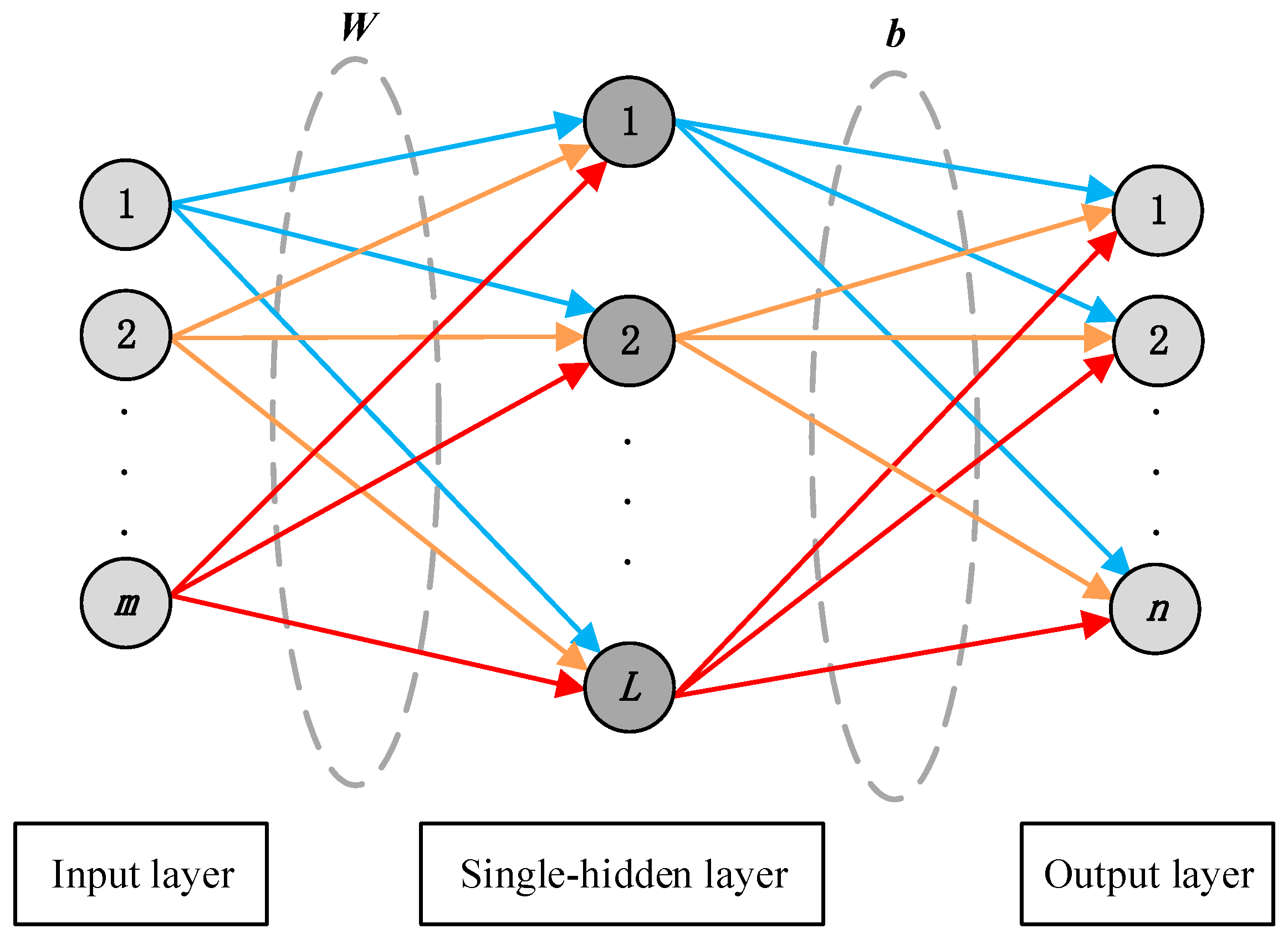
The extreme learning machines, proposed by Professor Huang [39], is a simple and efficient method for training single-hidden layer feedforward neural networks. It consists of an input layer, a hidden layer, and an output layer, as demonstrated in Figure 1.

For a given set of training samples $\mathrm{S}=(X_i,T_i)$, where $i=1,2,\dots ,N$, $X_i={[x_{i1},x_{i2},\dots x_{im}]}^T\in R^m$ and $T_i={[t_{i1},t_{i2},\dots t_{in}]}^T\in R^n$. $m,n$ are the input and output data dimensions respectively. Meanwhile, the model has a hidden layer neurons whose number is $L$. The hidden layer activation function is $g(•)$ and the input weight is $W_i=[W_{i1},W_{i2},\dots ,W_{im}]$. Then the network model can be expressed as:

$${\displaystyle \sum _{i=1}^L{\beta }_{i}g(W_i\cdot X_j+b_i)}=T_j^T,j=1,2,\dots ,N$$

(1)

where $b_i$ is the bias of the i-th neuron in the hidden layer. ${\beta }_i$ is the output weight vector between hidden layer nodes and output nodes, it can be expressed in terms of the matrix:

$$H\beta =T$$

(2)

where

$$H={\left[\begin{array}{ccc}g\left(W_1\cdot x_1+b_1\right)& \cdots & g\left(W_L\cdot x_1+b_L\right)\\ ⋮& \cdots & ⋮\\ g\left(W_1\cdot x_N+b_1\right)& \cdots & g\left(W_L\cdot x_N+b_L\right)\end{array}\right]}_{N\times L}$$

(3)

$$\beta ={\left[\begin{array}{c}{\beta }_1^T\\ ⋮\\ {\beta }_L^T\end{array}\right]}_{L\times n}, T={\left[\begin{array}{c}{T}_1^T\\ ⋮\\ T_N^T\end{array}\right]}_{N\times n}$$

(4)

The training of an ordinary extreme learning machines (OELM) is equivalent to the least squares norm solution of $\beta$, which can be written as follows:

$$\widehat{\beta }=H^{†}T$$

(5)

where $H^{†}$ is the Moore-Penrose generalized inverse of the hidden layer output matrix H.

The robust extreme learning machines based on the iteratively-reweighted-least-square method is to solve the problem of minimizing a loss function:

$$\underset{\beta }{\min }:{\Vert H\beta -T\Vert }^2$$

(6)

The output weight $\beta$ can be calculated according to Equation (7).

$$\beta =\{\begin{array}{c}{\left(H^{T}H\right)}^{-1}{H}^{T}T,N\ge L\\ H^T{\left(H{H}^T\right)}^{-1}T,N<L\end{array}$$

(7)

To enhance the robustness of the extreme learning machines, the loss function (6) of the model is usually adjusted as follows using L₂ norms:

$$\underset{\beta }{\min }:\frac{1}{2}{\Vert \beta \Vert }_2^2+C\frac{1}{2}{{\displaystyle \sum _{i=1}^n\Vert {\xi }^{\left(i\right)}\Vert }}_2^{2}s.t.:{\displaystyle \sum _{j=1}^L{\beta }_{j}g(W_j\cdot X_i+b_j)}=T_i-{\xi }^{\left(i\right)}\forall i$$

(8)

where C is the regularization parameter that trades off the norm of output weights and least squares training error. Several studies indicate that the larger the value C, the more accurate the imitative effect. As a reference, C can be taken as $2\times {10}^{30}$. Then, training the extreme learning machines is correspond to solving a ridge regression problem. $\beta$ is calculated as:

$$\beta =\{\begin{array}{c}{\left(H^{T}H+\frac{I}{C}\right)}^{-1}{H}^{T}T,N\ge L\\ H^T{\left(H{H}^T+\frac{I}{C}\right)}^{-1}T,N<L\end{array}$$

(9)

In order to mitigate the effects of noisy data on the model, M-estimate loss function is introduced. The loss function is then written as Equation (10).

$$\underset{\beta }{\min }:r\left(\beta \right)+C{\widehat{\sigma }}^2{\displaystyle \sum _{i=1}^N\rho \left(\frac{{\xi }^{\left(i\right)}}{\widehat{\sigma }}\right)}s.t.:{\displaystyle \sum _{j=1}^L{\beta }_{j}g(W_j\cdot X_i+b_j)}=T_i-{\xi }^{\left(i\right)}\forall i$$

(10)

where $r(\beta )$ is the regularization item to improve the generalization ability, $\rho (•)$ is the robust loss function, and $\widehat{\sigma }$ is the preliminary estimate of scale. Usually, $\widehat{\sigma }$ is taken as MAR/0.6745, where MAR is the median absolute residual. The robust loss function $\rho (z)$, its gradient $\psi \left(Z\right)$, and corresponding weight function $w\left(z\right)$ are defined as:

$$\Psi \left(z\right)=\partial \rho \left(z\right)/\partial z$$

(11)

$$w\left(z\right)=\{\begin{array}{c}\Psi \left(z\right)/z,z\ne 0\\ {\Psi }^{\prime }\left(0\right),z=0\end{array}$$

(12)

Five frequently used robust loss functions, their corresponding gradients and weight functions are listed in

Table 1. Robust loss function and its gradient and weight function.

Method	$\mathbf{Robust}\mathbf{Loss}\mathbf{Function}\mathit{\rho }\left(\mathit{z}\right)$	$\mathbf{Gradient}\mathbf{\Psi }\left(\mathit{z}\right)$	$\mathbf{Weight}\mathbf{Function}\mathit{w}\left(\mathit{z}\right)$	$\mathit{k}$
L1-norm	$\left|z\right|$	$sign\left(z\right)$	$\frac{1}{\max (\left|z\right|,\epsilon )},\epsilon ={10}^{-6}$	$-$
L2-norm	$\frac{1}{2}{z}^2$	$z$	1	$-$
Huber	$\{\begin{array}{c}\frac{1}{2}{\left(z\right)}^2,\left|z\right|\le k\\ k\left(\left|z\right|-k/2\right),\left|z\right|>k\end{array}$	$\{\begin{array}{c}z,\left|z\right|<k\\ k\cdot sign\left(z\right),\left|z\right|\ge k\end{array}$	$\min \left(1,\frac{k}{\left|z\right|}\right)$	1.345
Bsquare	$\{\begin{array}{c}\frac{1}{6}{k}^2\left(1-{\left(1-{\left(\frac{z}{k}\right)}^2\right)}^3\right),\left|z\le k\right|\\ \frac{1}{6}{k}^2,\left|z\right|>k\end{array}$	$z{\left(1-{\left(\frac{z}{k}\right)}^2\right)}^2\cdot I\left(\left|z\right|\le k\right)$	${\left(1-{\left(\frac{z}{k}\right)}^2\right)}^2\cdot I\left(\left|z\right|\le k\right)$	4.685
Welsch	$k^2\left(1-\exp \left(-\frac{1}{2}{\left(\frac{z}{k}\right)}^2\right)\right)$	$z\exp \left(-\frac{1}{2}{\left(\frac{z}{k}\right)}^2\right)$	$\exp \left(-\frac{1}{2}{\left(\frac{z}{k}\right)}^2\right)$	2.985

.

There are two most commonly used ways for regularization items $r(\beta )$: L₂ norm regularization and L₁ norm regularization. Given that the output data is one-dimensional, the algorithm to determine the output weight $\beta$ can be formulated as follows:

(1)

Extreme learning machines with L₂ norm regularization

The loss function in Equation (10) can be expressed as follows using L₂ norm regularization term:

$$\underset{\beta }{\min }:\frac{1}{2}{\Vert \beta \Vert }_2^2+C{\widehat{\sigma }}^2{\displaystyle \sum _{i=1}^n\rho \left(\frac{{\xi }^{\left(i\right)}}{\widehat{\sigma }}\right)}s.t.:{\displaystyle \sum _{j=1}^L{\beta }_{j}g(W_j\cdot X_i+b_j)}=T_i-{\xi }^{\left(i\right)}\forall i$$

(13)

The output weight $\beta$ can be solved according to the optimization theory as:

$$\beta =\{\begin{array}{c}{\left(\frac{I}{C}+H^T{W}_{N}H\right)}^{-1}{H}^T{W}_{N}T,N\ge L\\ H^T{\left(\frac{I}{C}+W_{N}H{H}^T\right)}^{-1}{W}_{N}T,N<L\end{array}$$

(14)

where $W_N=diag\left(w\left(\frac{{\xi }^{\left(1\right)}}{\widehat{\sigma }}\right),w\left(\frac{{\xi }^{\left(2\right)}}{\widehat{\sigma }}\right),\dots ,w\left(\frac{{\xi }^{\left(N\right)}}{\widehat{\sigma }}\right)\right)$ denotes the sample weights.

(2)

Extreme learning machines with L₁ norm regularization

The loss function in Equation (10) can be expressed as the following use the L₁ norm regularization term:

$$\underset{\beta }{\min }:{\Vert \beta \Vert }_1+C{\widehat{\sigma }}^2{\displaystyle \sum _{i=1}^n\rho \left(\frac{{\xi }^{\left(i\right)}}{\widehat{\sigma }}\right)}s.t.:{\displaystyle \sum _{j=1}^L{\beta }_{j}g(W_j\cdot X_i+b_j)}=T_i-{\xi }^{\left(i\right)}\forall i$$

(15)

The output weight $\beta$ can be solved iteratively according to the optimization theory as:

$$\beta =\{\begin{array}{c}{\left(\frac{W_L}{C}+H^T{W}_{N}H\right)}^{-1}{H}^T{W}_{N}T,N\ge L\\ W_L^{-1}{H}^T{\left(\frac{I}{C}+W_{N}H{W}_L^{-1}{H}^T\right)}^{-1}{W}_{N}T,N<L\end{array}$$

(16)

where $W_L=diag\left(w_{L_1}\left({\beta }_1\right),w_{L_1}\left({\beta }_2\right),\dots ,w_{L_1}\left({\beta }_L\right)\right)$ denotes the weights of hidden nodes and $W_N=diag\left(w\left(\frac{{\xi }^{\left(1\right)}}{\widehat{\sigma }}\right),w\left(\frac{{\xi }^{\left(2\right)}}{\widehat{\sigma }}\right),\dots ,w\left(\frac{{\xi }^{\left(N\right)}}{\widehat{\sigma }}\right)\right)$ denotes the samples weights.

3. Structural Reliability Analysis Based on the IRLS-ELM and the MCS

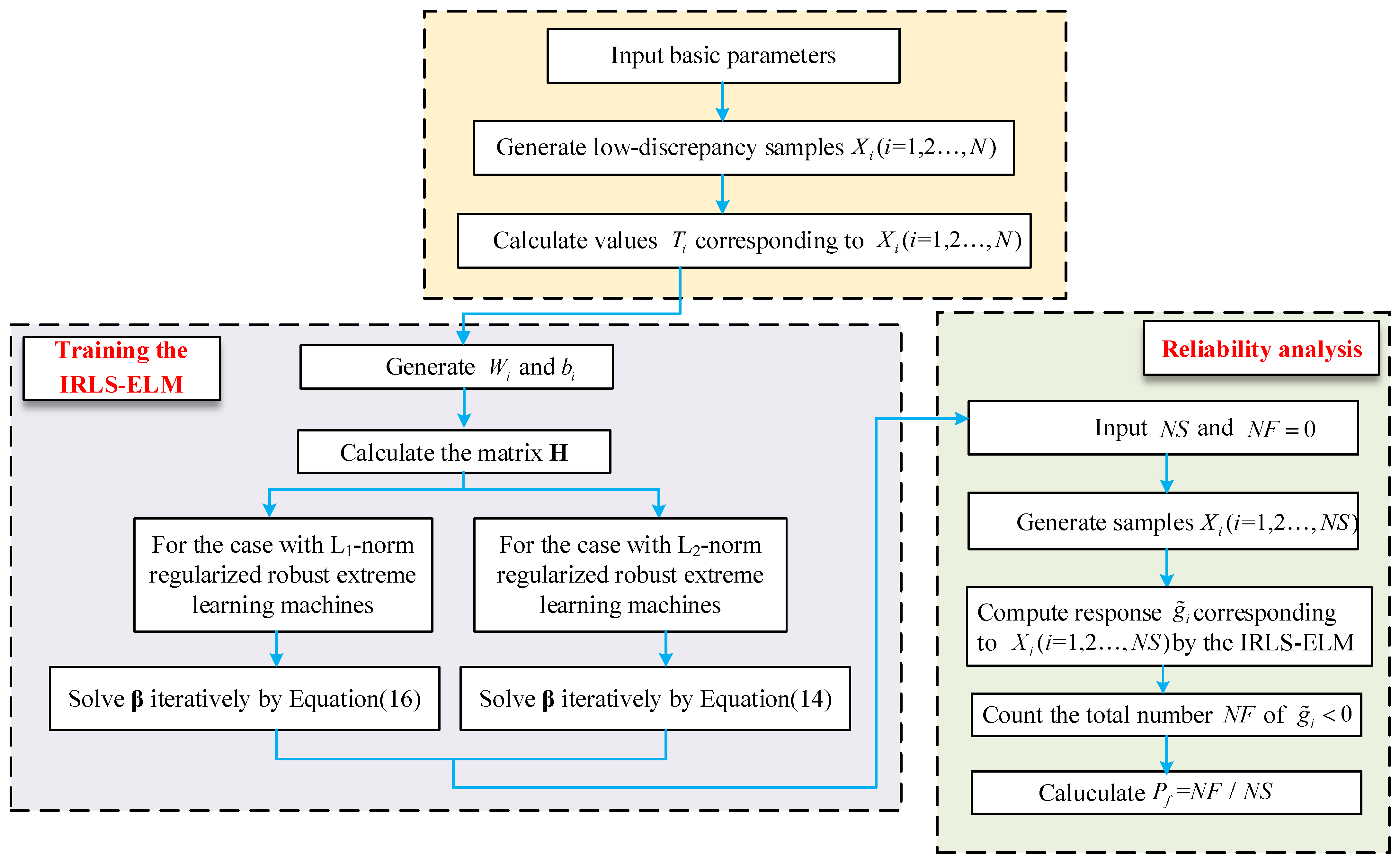
In this paper, the IRLS-ELM in combination with the MCS is used to analyze structural reliability. The algorithm is shown in Figure 2. The following steps provide details about the algorithm.

Step 1. Input basic parameters including the number of samples $N$, the number of hidden layer neurons of the neural network $L$, and the number of random variables m.

Step 2. Construct the training samples: The low-discrepancy samples $X_i(i=1,\cdots ,N)$ are obtained by the probability distribution of random variables from the Latin hypercube, the Halton Quasi random sequence, and etc. Accordingly, the structural response and the performance function values $T_i(i=1,\cdots ,N)$ can be calculated.

Step 3. Train extreme learning machines: In the first place, the random input weight matrix $W_i=[W_{i1},\cdots ,W_{im}]$ and the hidden layer offset $b_i(i=1,\cdots ,N)$ are generated randomly. Then the Equation (3) is used to calculate the matrix $H$. For the case of L₂-norm regularized robust extreme learning machines, Equation (14) is employed to solve the output weight vector $\beta$ of the extreme learning machines iteratively. For the case of L₁-norm regularized robust extreme learning machines, the output weight vector $\beta$ is evaluated by Equation (16).

Step 4. Structural reliability analysis: Input the number of samples in the MCS $NS$ and the sample counter in the failure domain $NF$. $NF$ is set to be 0. The samples $X_i(i=1,\cdots ,NS)$ are generated in terms of the distribution of random variables. The response ${\widehat{g}}_i$ of the samples $X_i(i=1,\cdots ,NS)$ are computed by the obtained extreme learning machines. The number of ${\widehat{g}}_i<0$ is iteratively counted as $NF$. In the end, the failure probability is calculated as $P_f=NF/NS$.

4. Numerical Examples

In this section, four examples are illustrated below. In order to facilitate the analysis, the sample sizes are defined as N = 100 and the number of hidden layer neurons is taken as 60. Two regularization methods and five robust loss functions form ten combinations of the IRLS-ELM for these examples. For the sake of description, the names of these ten combinations are abbreviated and listed in

Table 2. Ten combination methods and their name abbreviations.

Regularization Methods	Robust Loss Function Type	Name Abbreviations
L1 regularization method	L1 norm	L1-L1
	L2 norm	L1-L2
	Huber	L1-H
	Bisquare	L1-B
	Welsch	L1-W
L2 regularization method	L1 norm	L2-L1
	L2 norm	L2-L2
	Huber	L2-H
	Bisquare	L2-B
	Welsch	L2-W

. The ordinary extreme learning machines, as a comparison, is also abbreviated as the OELM. In addition, the answer of the MCS is regarded as the most accurate.

4.1. Example 1

A highly non-linear performance function

$$g\left(X\right)=567X_1{X}_2-0.5X_3^2=0$$

(17)

contains three non-normal random variables and their distribution parameters are presented in

Table 3. Random variables and their distribution in Example 1.

Variable	Means	Variable Coefficient	Distribution
$X_1$	0.6	0.131	Normal
$X_2$	2.18	0.03	Type I extreme value for maxima
$X_3$	32.8	0.03	Lognormal

.

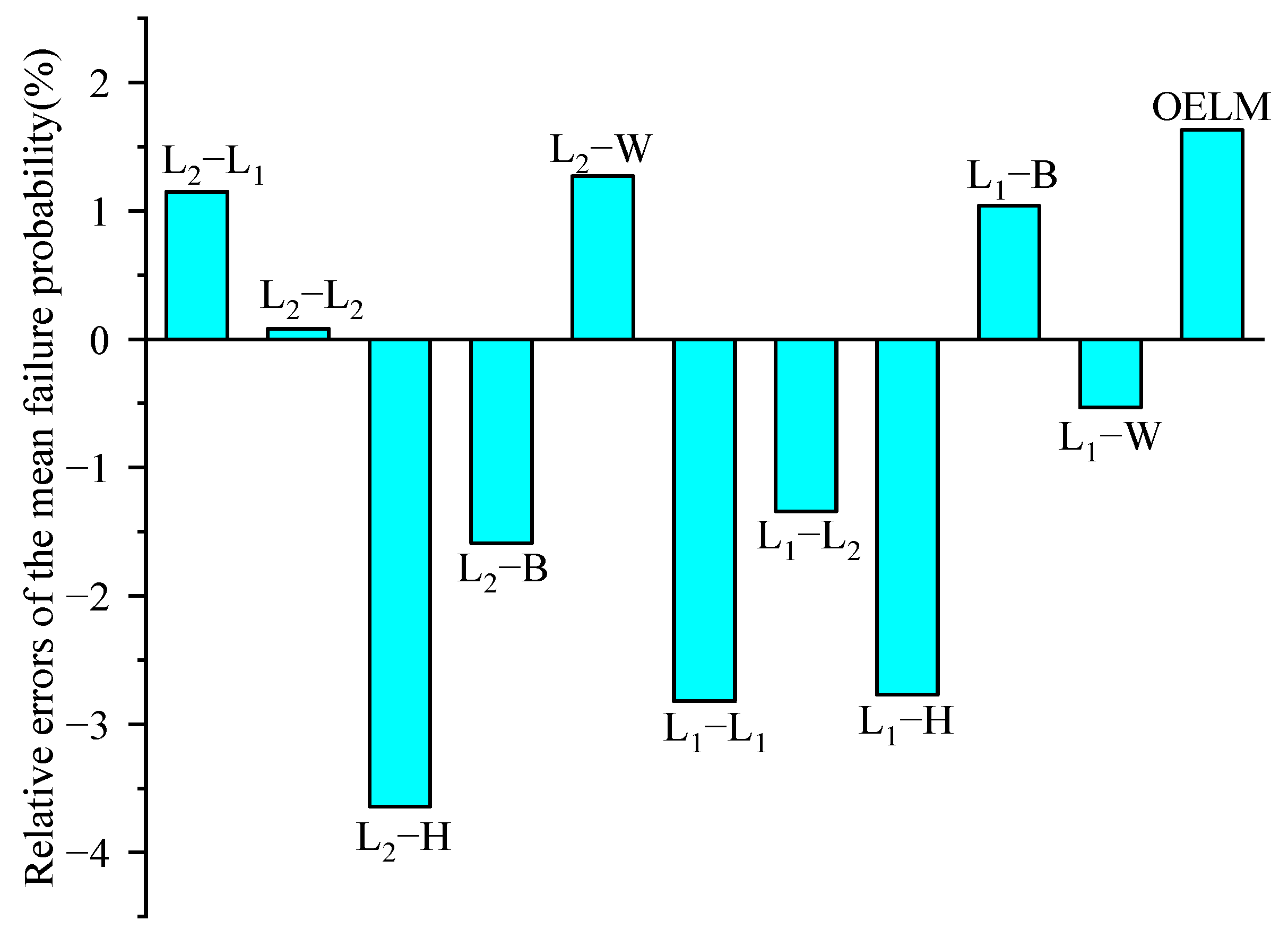
The means of failure probability and its standard deviations calculated by these ten combinations of the IRLS-ELM, along with the traditional MCS and the OELM are given in

Table 4. The mean and its standard deviation of failure probability in Example 1.

Method	Failure Probability		Method	Failure Probability
	Mean	Standard Deviation		Mean	Standard Deviation
MCS	0.025215	0.00022	L2-L1	0.025606	0.00022
L1-L1	0.024504	0.00022	L2-L2	0.025234	0.00022
L1-L2	0.024878	0.00022	L2-H	0.024298	0.00022
L1-H	0.024516	0.00022	L2-B	0.024814	0.00022
L1-B	0.025476	0.00022	L2-W	0.025534	0.00022
L1-W	0.025082	0.00022	OELM	0.024804	0.00022

. The coefficient of variation is less than 0.9% for all these ten combinations of the IRLS-ELM. The results of failure probability show little dispersion. The failure probability yielded by the MCS is 0.025215 with 10⁶ samples. The relative error of failure probability obtained by the ten combined methods is shown in Figure 3. It can be seen that the combination L₂-L₂ yields the most accurate mean failure probability with the relative error 0.08%. The relative error of the OELM is 1.62%, which has lower accuracy than the combination L₂-L₁, L₂-L₂, L₂-B, L₂-W, L₁-L₂, L₁-B, and L₁-W. The relative error of the combination L₂-L₁, L₂-B, L₂-W, L₁-L₁, L₁-L₂, L₁-H and L₁-B is varying between 1–3%. Additionally, the combination L₂-H achieves the largest relative error 3.64%.

4.2. Example 2

Consider the following performance function

$$G\left(u\right)=\exp \left[0.4\left(u_1+2\right)+6.2\right]-\exp \left(0.3u_2+5\right)-200$$

(18)

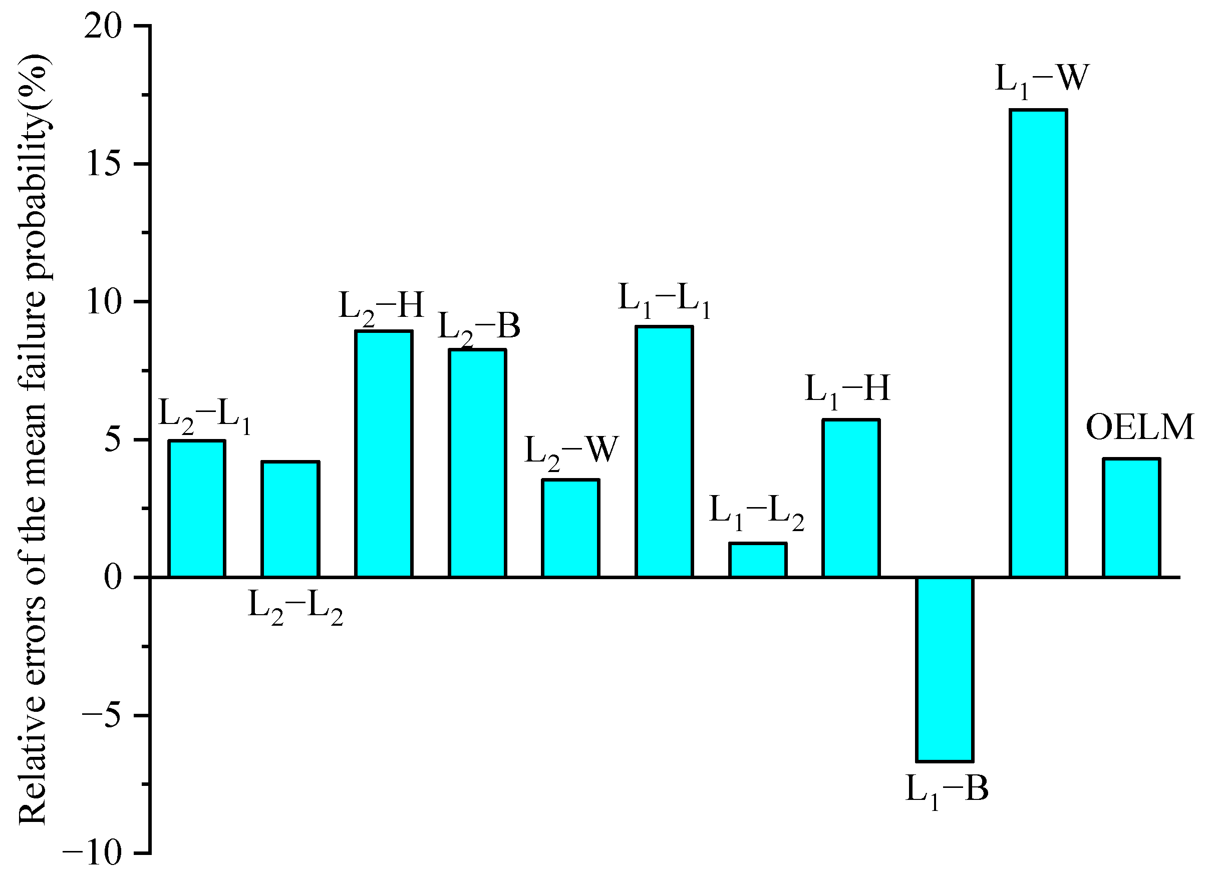
where $u_1$, $u_2$ are independent random variables with normal distribution $u_1~N\left(0,1\right)$, $u_2~N\left(0,1\right)$. The failure probability using the MCS is 0.003715 with the sample size 10⁶. The means of failure probability and its standard deviations using ten combinations of the IRLS-ELM are shown in

Table 5. The mean and its standard deviation of failure probability in Example 2.

Method	Failure Probability		Method	Failure Probability
	Mean	Standard Deviation		Mean	Standard Deviation
MCS	0.003715	0.000061	L2-L1	0.003899	0.000062
L1-L1	0.004053	0.000064	L2-L2	0.003871	0.000062
L1-L2	0.003761	0.000064	L2-H	0.004047	0.000063
L1-H	0.003927	0.000063	L2-B	0.004022	0.000063
L1-B	0.003467	0.000059	L2-W	0.003846	0.000062
L1-W	0.004345	0.000066	OELM	0.003554	0.00006

. The relative error of failure probability obtained by ten methods and the OELM, compared with the result by MCS, are exhibited in Figure 4. The coefficient of variation is less than 1.7% for all these ten combinations of the IRLS-ELM. The results of failure probability show less dispersion.

From the Table 5 and Figure 4, it can be observed that among the ten combination methods, the combination L₁-L₂ has the minimum relative error. The relative errors of failure probability calculated by the combination L₂-L₁, L₂-L₂, L₂-W and OELM are less than 5% with satisfactory accuracy. The relative errors obtained by the combination L₂-H, L₂-B, L₁-L₁, L₁-H and L₁-B are found to be slightly larger but within 10%. The relative error of the OELM is 4.3%. Compared with the OELM, the combination L₂-L₂, L₂-W, and L₁-L₂ have higher accuracy. The combination L₁-W stands out in delivering relative error beyond 15%.

4.3. Example 3

A series structure system with three main failure modes and three performance functions are written as:

$$Z_1=\left(Y_1+Y_2-Y_3\right)/\sqrt{3}+2.0$$

(19)

$$Z_2=\left(Y_1-Y_3\right)/\sqrt{2}+3.4$$

(20)

$$Z_3=\left(Y_2-Y_3\right)/\sqrt{2}+3.6$$

(21)

where $Y_1,Y_2,Y_3$ are independent standard normal random variables. $Y_1~N\left(0,1\right)$, $Y_2~N\left(0,1\right)$, $Y_3~N\left(0,1\right)$.

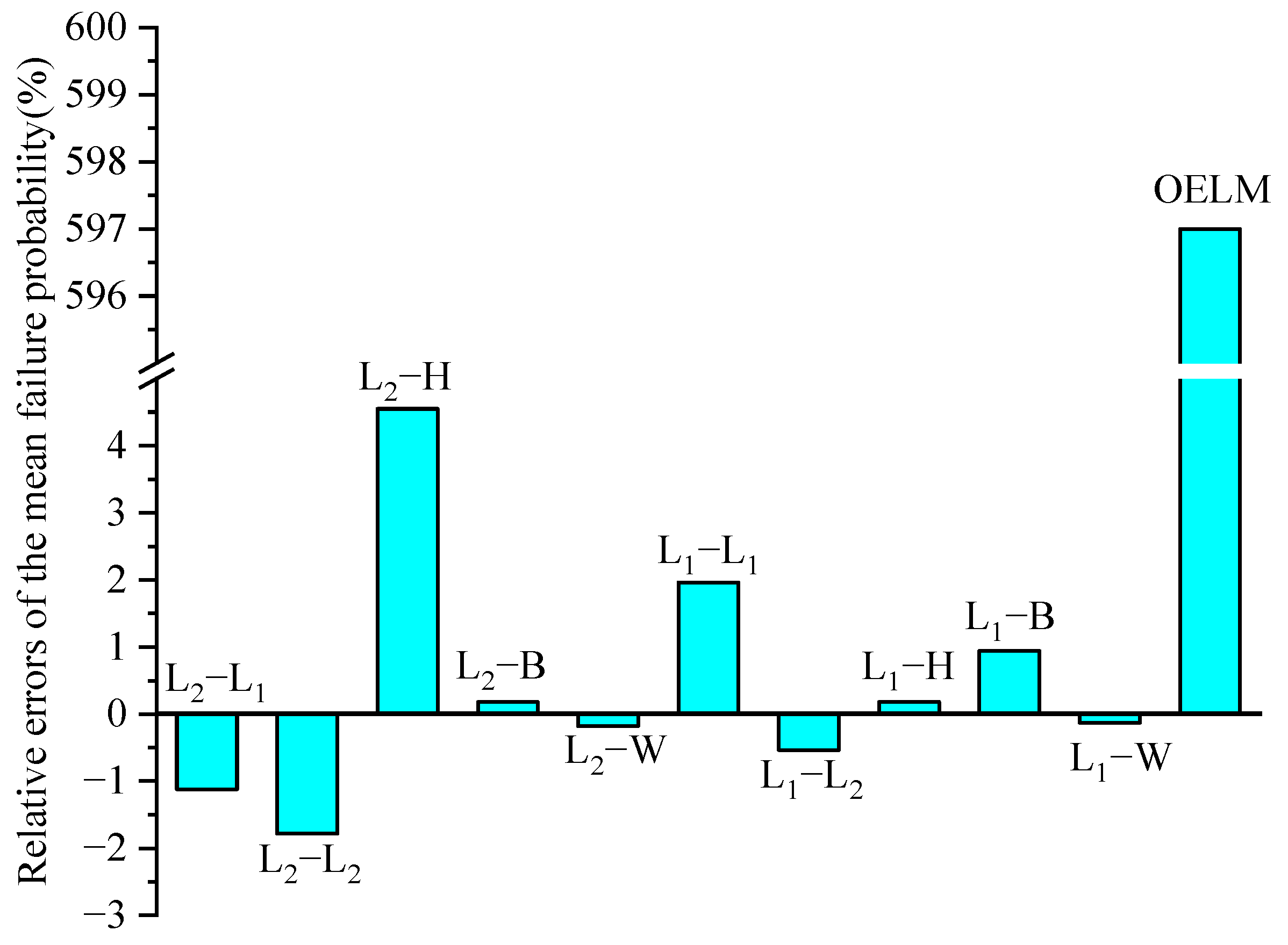
In

Table 6. The mean and its standard deviation of failure probability in Example 3.

Method	Failure Probability		Method	Failure Probability
	Mean	Standard Deviation		Mean	Standard Deviation
MCS	0.02241	0.00047	L2-L1	0.02216	0.00047
L1-L1	0.02285	0.00047	L2-L2	0.02201	0.00047
L1-L2	0.02229	0.00047	L2-H	0.02343	0.00048
L1-H	0.02245	0.00047	L2-B	0.02245	0.00047
L1-B	0.02262	0.00047	L2-W	0.02237	0.00047
L1-W	0.02238	0.00047	OELM	0.1562	0.0011

, the means of failure probability and its standard deviations using ten combinations of the IRLS-ELM are presented. Simultaneously, the relative errors of the failure probability yielded by different methods, compared to the result by MCS, are displayed in Figure 5. The coefficient of variation is less than 2.2% for all these ten combinations of the IRLS-ELM. We can observe that the answer of the combination L₁-W is in agreement with that of the MCS, whose relative error is only 0.13%. The combination L₂-B, L₂-W and L₁-W also have high accuracy, with the relative error 0.18%, while the OELM gives a wrong answer with relative error 597%.

4.4. Example 4

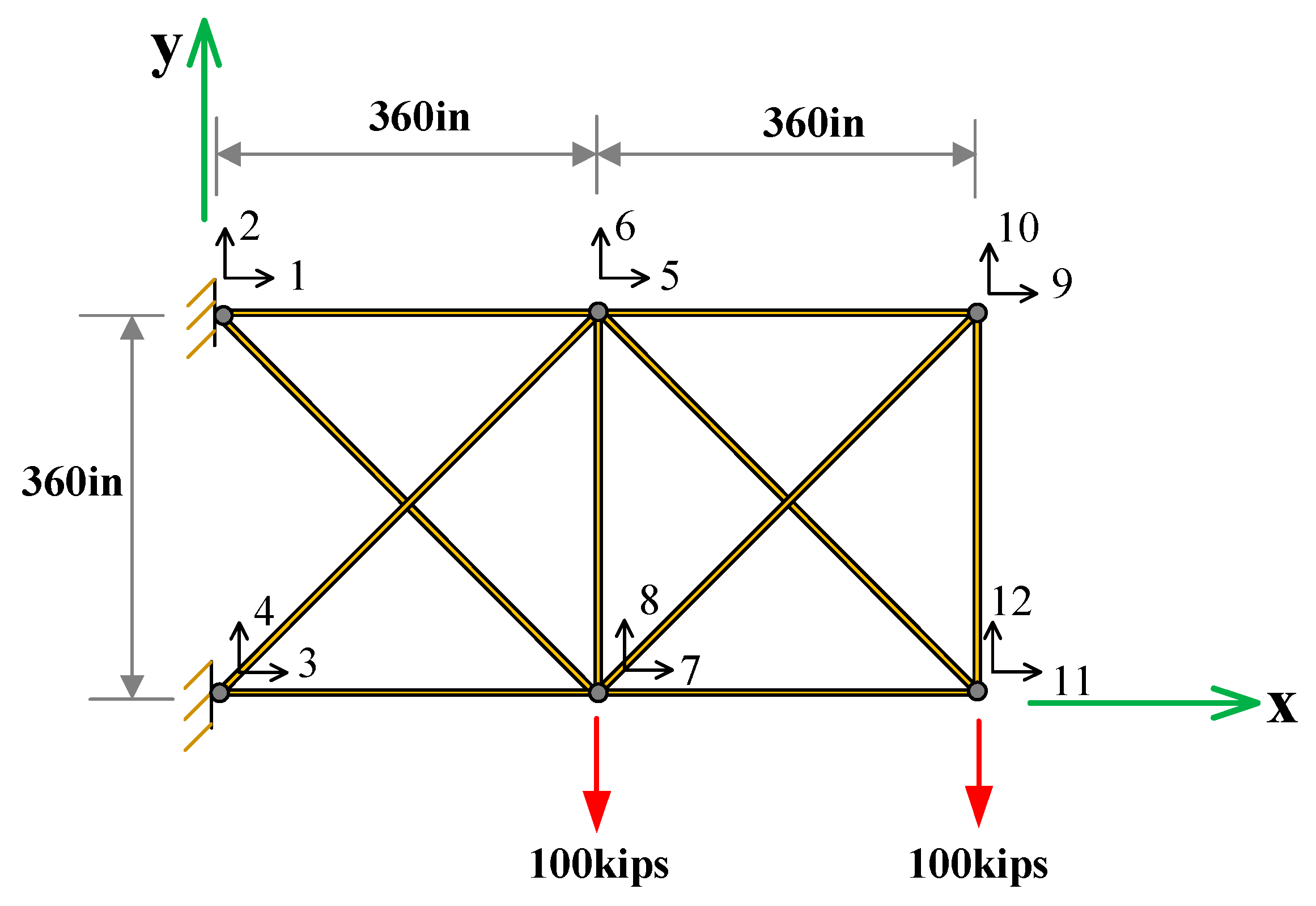
As shown in Figure 6, a ten-bar truss structure is considered. The area of each bar is denoted by $A_i\left(i=1,2,\dots ,10\right)$ which follows the same normal distribution $N\left(10,{0.5}^2\right)$, $A_i~N\left(10,{0.5}^2\right),(i=1,2,\dots ,10)$ namely. The allowable value of structural stress is ${\sigma }_{allow}=2.1\times {10}^4$. Generally, the structure as invalid is defined when the stress value of any bar is greater than the allowable value, which ${\sigma }_i>{\sigma }_{allow}(i=1,2,\dots ,10)$.

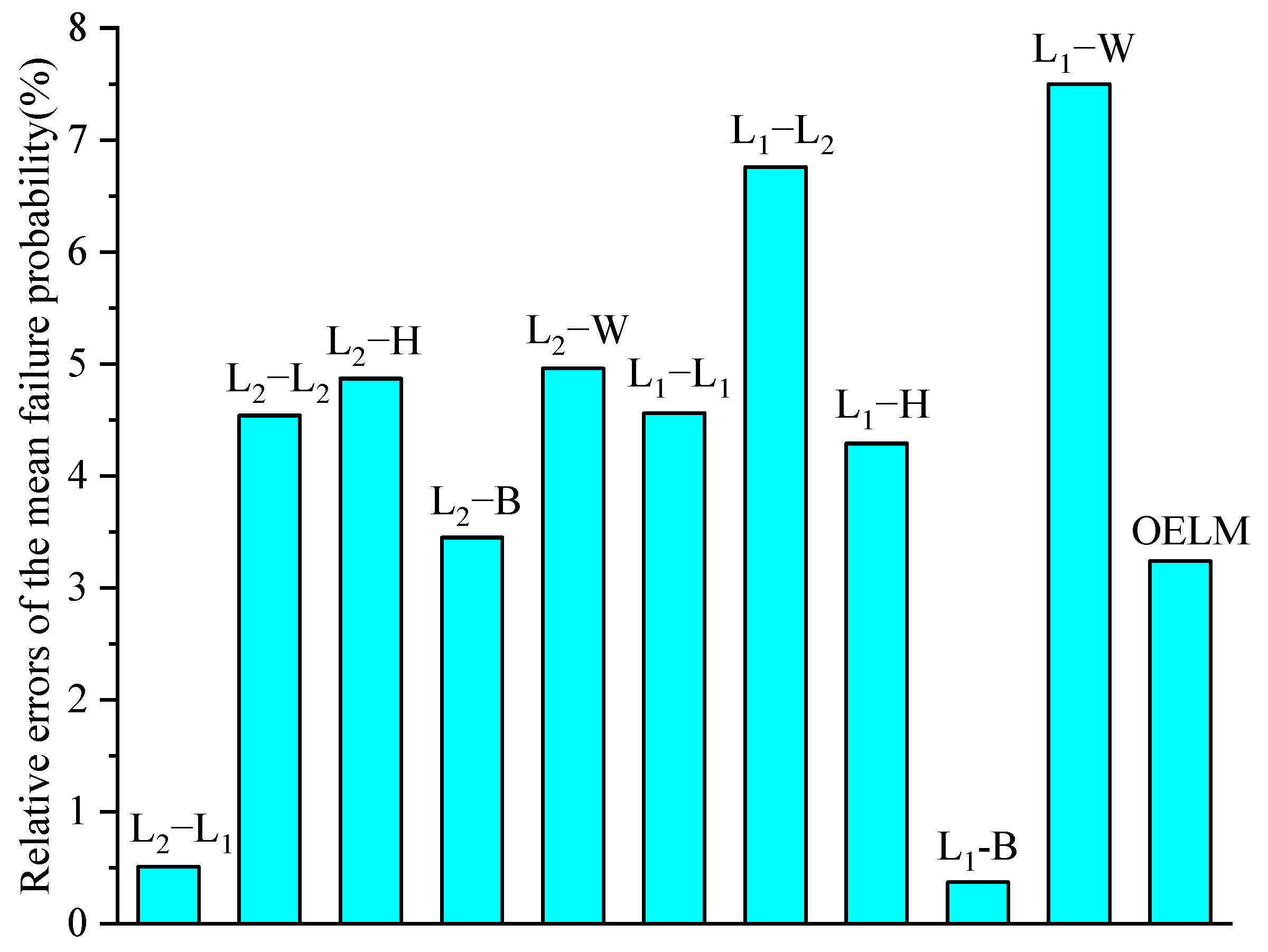
The means of failure probability and its standard deviations using ten combinations of the IRLS-ELM are represented in

Table 7. The mean and its standard deviation of failure probability in Example 4.

Method	Failure Probability		Method	Failure Probability
	Mean	Standard Deviation		Mean	Standard Deviation
MCS	0.06562	0.00035	L2-L1	0.065954	0.00035
L1-L1	0.068612	0.00036	L2-L2	0.068596	0.00036
L1-L2	0.070054	0.00036	L2-H	0.068818	0.00036
L1-H	0.068438	0.00036	L2-B	0.067884	0.00036
L1-B	0.065862	0.00035	L2-W	0.068876	0.00036
L1-W	0.07054	0.00036	OELM	0.067752	0.00036

. The relative errors of failure probability calculated by ten combination methods and the OELM compared with the result by the MCS are depicted in Figure 7. The coefficient of variation is less than 0.5% for all these ten combinations of the IRLS-ELM. It can be found that the failure probability by the combination L₁-B is very close to the result by the MCS, that is to say, the relative error of the combination L₁-B is nearly zero. Besides, the combination L₂-L₂, L₂-H, L₂-B, L₂-W, L₁-L₁, and L₁-H have good accuracy with the relative errors below 5%. The relative error of the OELM is 3.24%. The relative errors of the combination L₁-L₂ and L₁-W are greater than 5% but less than 10%. Most typically, the relative error of the combination L₁-W reaches 7.5%.

5. Discussion

Different loss functions together with two regularization approaches are combined for reliability analysis in the IRLS-ELM. The ranks of these combinations in terms of the mean relative error of failure probability for the above four numerical examples are listed in ascending order in

Table 8. Rank of the ten methods in terms of the relative error of failure probability.

Example	Method (in Ascending Order of the Relative Error)
1	L2-L2	L1-W	L1-B	L2-W	L1-L2	L2-L1	L2-B	L1-H	L1-L1	L2-H
2	L1-L2	L2-W	L2-L2	L2-L1	L1-H	L1-B	L2-B	L2-H	L1-L1	L1-W
3	L1-W	L2-B	L2-W	L1-H	L1-L2	L1-B	L2-L1	L2-L2	L1-L1	L2-H
4	L1-B	L2-L1	L2-B	L1-H	L2-L2	L1-L1	L2-H	L2-W	L1-L2	L1-W

The relative error of the bolded method is less than 5%.

. The methods with the mean relative error less than 5% are marked in bold.

Table 9. Minimum error and maximum relative errors for the four examples.

Example	Minimum Error		Method	Maximum Error
	Method	Mean Relative Error (%)		Mean Relative Error (%)
1	L2-L2	0.08	L2-H	−3.64
2	L1-L2	1.24	L1-W	16.96
3	L1-W	−0.13	L2-H	4.55
4	L1-B	0.37	L1-W	7.50

summarizes the maximum and minimum relative errors and the corresponding methods for each example. We can see that: the combination L₂-L₂ and L₂-W are ranked in the top five with the minimum relative errors with the relative error below 5%. It indicates that these two combinations are more accurate than the others in reliability analysis. Conversely, the combination L₁-W exhibits relative instability with the relative error more than 15% in Example 2, less than 1% in Example 3. The OELM even gives a wrong answer with the relative error more than 500% in Example 3 despite less than 5% in the other examples. The most accurate relative error of the combination L₁-W 0.13% is observed in Example 3.

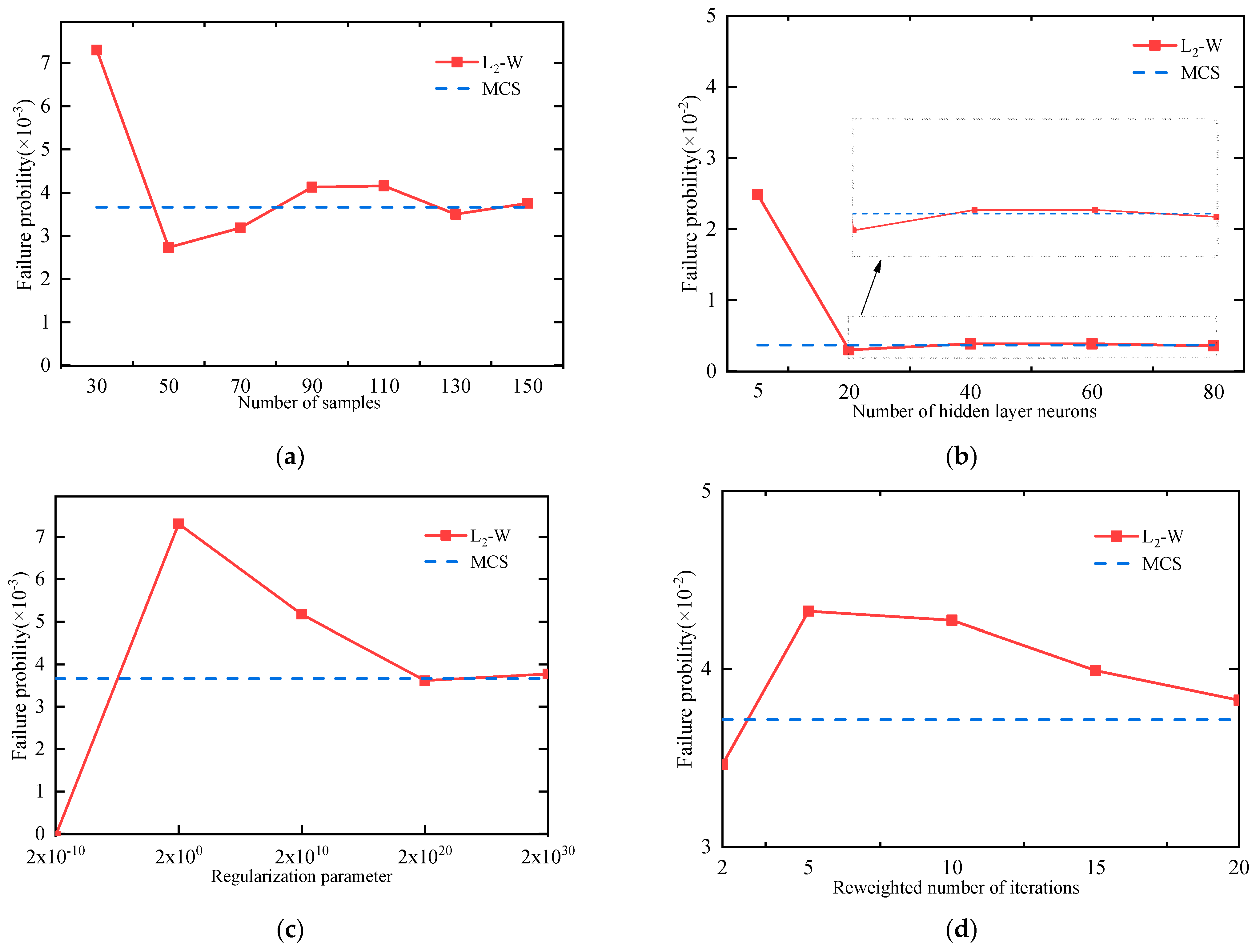
In order to explore the effects of parameters on the accuracy of structural failure probability involved in the above algorithm for reliability analysis, including the number of samples N, the number of hidden layer neurons L, the regularization parameters C and the reweighted number of iterations t. The L₂-W method for Example 2 is taken as an illustration to find the underlying regularity. The variation trend of mean failure probability with respect to the parameters compared with the MCS is shown in Figure 8.

Table 10. The mean failure probability and its relative error for different number of samples.

Sample Sizes N	Mean of the Failure Probability	Relative Error
30	0.007349	97.82%
50	0.002784	−25.06%
70	0.003236	−12.89%
90	0.004179	−12.49%
110	0.004204	13.16%
130	0.003551	−4.41%
150	0.003806	2.45%

,

Table 11. The mean failure probability and its relative error for different number of hidden layer neurons.

Number of the Hidden Layer Neurons L	Mean of the Failure Probability	Relative Error
5	0.024829	568.34%
20	0.003011	−18.95%
40	0.003868	4.12%
60	0.003871	4.20%
80	0.003581	3.61%

,

Table 12. The mean failure probability and its relative error for different regularization parameters.

Regularization Parameter C	Mean of the Failure Probability	Relative Error
$2\times {10}^{-10}$	0	-
2	0.00736	98.12%
$2\times {10}^{10}$	0.005226	40.67%
$2\times {10}^{20}$	0.003664	1.37%
$2\times {10}^{30}$	0.003824	2.93%

and

Table 13. The mean failure probability and its relative error for different reweighted number of iterations.

Number of Iterations t	Mean of the Failure Probability	Relative Error
2	0.003463	−6.78%
5	0.004324	16.39%
10	0.004273	15.02%
15	0.003991	7.43%
20	0.003824	2.93%

present the mean failure probabilities and their relative error in Example 2 for different parameters with different values.

It can be found that, with the increase of the number of samples N, the error of failure probability gradually decreases. When the number of samples increases to 130, the relative error of the mean failure probability is less than 5%. It demonstrates that a relatively large number of samples is critical to obtain a satisfactory accuracy on failure probability by the IRLS-ELM. Likewise, we can conclude from the Table 11 that, as the number of hidden layer neurons increases, the errors of failure probability decrease significantly. When the number of neurons reaches 40, the error of failure probability is less than 5%. It indicates that the number of neurons has an important role in determining the accuracy of failure probability. However, the neurons beyond a certain number have only a minor impact on the accuracy of failure probability. Generally, if the regularization parameter C is too small, least squares training error will not work and the algorithm will give an answer with a great error. From the Figure 8c we can see that the error of failure probability decrease as the C value increases. When the regularization parameters C equal 2 × 10²⁰, the relative error of failure probability is less than 2%. As the number of iterations t increases (shown in Table 13 and Figure 8d), the relative error of failure probability decreases. As the reweighted number of iterations increases to 20, the relative error of failure probability decreases to 2.93%.

6. Conclusions

The response surface method based on the IRLS-ELM, combined with the MCS for structural reliability analysis is conducted in this paper. In the case of highly nonlinear implicit performance functions in engineering, the IRLS-ELM shows good generalization performance and high efficiency, more accurate and robust than the OELM. It achieves this by introducing L₁, L₂ norm, Huber, Bisquare, and Welsch loss function to enhance the robustness, and L₁ and L₂ norm regularization method of output weight to avoid overfitting. Four examples are used to compare the accuracy of failure probability employing ten methods that utilize different combinations of loss functions and regularization methods of the IRLS-ELM. In addition, the accuracy of failure probability will be affected by the parameters, including the number of samples N, the number of neurons L, the regularization parameters C, and the reweighted number of iterations t. Some concluding remarks are as follows:

(1)

For those highly nonlinear performance functions, an appropriate number of samples and hidden layer neurons are critical to obtaining high accuracy in structural failure probability for the proposed algorithm to perform reliability analysis. Too few samples or too few hidden layer neurons will result in lower accuracy. An excess of samples or hidden layer neurons has little significance in improving the accuracy of the failure probability. If the regularization parameter C is too small or the reweighted number of iterations is not enough, it is difficult to obtain the failure probability with satisfactory accuracy. Generally, it is suggested that the regularization parameter C is taken as 2 × 10²⁰ and the reweighted number of iterations is set to 20.

(2)

The loss function and regularization method also affect the accuracy of the failure probability. The combination chosen of the loss function and regularization method may have an important influence on the accuracy of final results of structural failure probability. The results of the above numerical examples indicate that the combination of L₂-L₂ and L₂-W yields more accuracy than the other combinations. To sum up, the relative error of failure probability in the combinations of L₂ norm regularization and L₂ norm or Welsch loss function is less than 5%, while the other combinations exhibit more dispersity in the accuracy of failure probability for different problems.

References

- Yang, D.; Li, G.; Cheng, G. Convergence Analysis of First Order Reliability Method Using Chaos Theory. Comput. Struct. 2006, 84, 563–571. [Google Scholar] [CrossRef]
- Meng, Z.; Li, G.; Yang, D.; Zhan, L. A New Directional Stability Transformation Method of Chaos Control for First Order Reliability Analysis. Struct. Multidiscp. Optim. 2017, 55, 601–612. [Google Scholar] [CrossRef]
- Keshtegar, B.; Meng, Z. A Hybrid Relaxed First-Order Reliability Method for Efficient Structural Reliability Analysis. Struct. Saf. 2017, 66, 84–93. [Google Scholar] [CrossRef]
- Du, X.; Zhang, J. Second-Order Reliability Method with First-Order Efficiency. In Proceedings of the Volume 1: 36th Design Automation Conference, Parts A and B, ASMEDC, Montreal, QC, Canada, 15–18 August 2010; pp. 973–984. [Google Scholar]
- Li, G.; Li, B.; Hu, H. A Novel First–Order Reliability Method Based on Performance Measure Approach for Highly Nonlinear Problems. Struct. Multidiscp. Optim. 2018, 57, 1593–1610. [Google Scholar] [CrossRef]
- Hu, Z.; Du, X. First Order Reliability Method for Time-Variant Problems Using Series Expansions. Struct. Multidiscp. Optim. 2015, 51, 1–21. [Google Scholar] [CrossRef]
- Dudzik, A.; Potrzeszcz-Sut, B. Hybrid Approach to the First Order Reliability Method in the Reliability Analysis of a Spatial Structure. Appl. Sci. 2021, 11, 648. [Google Scholar] [CrossRef]
- Zhao, G.; Li, Y.; Zhang, B. Asymptotic Analysis Methods for Structural Reliability. J. Dalian Univ. Technol. 1995, 4, 442–447. [Google Scholar]
- Aslett, L.J.M.; Nagapetyan, T.; Vollmer, S.J. Multilevel Monte Carlo for Reliability Theory. Reliab. Eng. Syst. Saf. 2017, 165, 188–196. [Google Scholar] [CrossRef] [Green Version]
- Liu, X.; Zheng, S.; Wu, X.; Chen, D.; He, J. Research on a Seismic Connectivity Reliability Model of Power Systems Based on the Quasi-Monte Carlo Method. Reliab. Eng. Syst. Saf. 2021, 215, 107888. [Google Scholar] [CrossRef]
- Xu, J.; Zhang, W.; Sun, R. Efficient Reliability Assessment of Structural Dynamic Systems with Unequal Weighted Quasi-Monte Carlo Simulation. Comput. Struct. 2016, 175, 37–51. [Google Scholar] [CrossRef]
- Changcong, Z.; Zhenzhou, L.; Feng, Z.; Zhufeng, Y. An Adaptive Reliability Method Combining Relevance Vector Machine and Importance Sampling. Struct. Multidiscp. Optim. 2015, 52, 945–957. [Google Scholar] [CrossRef]
- Fan, W.; Liu, R.; Ang, A.H.-S.; Li, Z. A New Point Estimation Method for Statistical Moments Based on Dimension-Reduction Method and Direct Numerical Integration. Appl. Math. Model. 2018, 62, 664–679. [Google Scholar] [CrossRef] [Green Version]
- Zhao, Y.-G.; Zhang, X.-Y.; Lu, Z.-H. A Flexible Distribution and Its Application in Reliability Engineering. Reliab. Eng. Syst. Saf. 2018, 176, 1–12. [Google Scholar] [CrossRef]
- Lu, Z.; Song, J.; Song, S.; Yue, Z.; Wang, J. Reliability Sensitivity by Method of Moments. Appl. Math. Model. 2010, 34, 2860–2871. [Google Scholar] [CrossRef]
- Zhao, Y.-G.; Ono, T. Moment Methods for Structural Reliability. Struct. Saf. 2001, 23, 47–75. [Google Scholar] [CrossRef]
- Engelund, S.; Rackwitz, R. A Benchmark Study on Importance Sampling Techniques in Structural Reliability. Struct. Saf. 1993, 12, 255–276. [Google Scholar] [CrossRef]
- Dai, H.; Zhang, H.; Wang, W. A New Maximum Entropy-Based Importance Sampling for Reliability Analysis. Struct. Saf. 2016, 63, 71–80. [Google Scholar] [CrossRef]
- Ibrahim, Y. Observations on Applications of Importance Sampling in Structural Reliability Analysis. Struct. Saf. 1991, 9, 269–281. [Google Scholar] [CrossRef]
- Jahani, E.; Shayanfar, M.A.; Barkhordari, M.A. A New Adaptive Importance Sampling Monte Carlo Method for Structural Reliability. KSCE J. Civ. Eng. 2013, 17, 210–215. [Google Scholar] [CrossRef]
- Bjerager, P. Probability Integration by Directional Simulation. J. Eng. Mech. 1988, 114, 1285–1302. [Google Scholar] [CrossRef]
- Liu, P.-L.; Der Kiureghian, A. Optimization Algorithms for Structural Reliability. Struct. Saf. 1991, 9, 161–177. [Google Scholar] [CrossRef]
- Rackwitz, R.; Flessler, B. Structural Reliability under Combined Random Load Sequences. Comput. Struct. 1978, 9, 489–494. [Google Scholar] [CrossRef]
- Balesdent, M.; Morio, J.; Marzat, J. Kriging-Based Adaptive Importance Sampling Algorithms for Rare Event Estimation. Struct. Saf. 2013, 44, 1–10. [Google Scholar] [CrossRef]
- Choi, K.; Lee, G.; Lee, T.H.; Choi, D.-H.; Yoon, S.-J. A Sampling-Based Reliability-Based Design Optimization Using Kriging Metamodel with Constraint Boundary Sampling. In Proceedings of the 12th AIAA/ISSMO Multidisciplinary Analysis and Optimization Conference; American Institute of Aeronautics and Astronautics, Victoria, BC, Canada, 10–12 September 2008. [Google Scholar]
- Tang, K. Reliability-Based Structural Optimization Based on Kriging Method. Master’s Thesis, Shenyang Aerospace University, Shenyang, China, 2017. [Google Scholar]
- Hosni Elhewy, A.; Mesbahi, E.; Pu, Y. Reliability Analysis of Structures Using Neural Network Method. Probabilistic Eng. Mech. 2006, 21, 44–53. [Google Scholar] [CrossRef]
- Cheng, J.; Li, Q.S.; Xiao, R. A New Artificial Neural Network-Based Response Surface Method for Structural Reliability Analysis. Probabilistic Eng. Mech. 2008, 23, 51–63. [Google Scholar] [CrossRef]
- Deng, J.; Gu, D.; Li, X.; Yue, Z.Q. Structural Reliability Analysis for Implicit Performance Functions Using Artificial Neural Network. Struct. Saf. 2005, 27, 25–48. [Google Scholar] [CrossRef]
- Li, X.; Li, X.; Su, Y. A Hybrid Approach Combining Uniform Design and Support Vector Machine to Probabilistic Tunnel Stability Assessment. Struct. Saf. 2016, 61, 22–42. [Google Scholar] [CrossRef]
- Alibrandi, U.; Alani, A.M.; Ricciardi, G. A New Sampling Strategy for SVM-Based Response Surface for Structural Reliability Analysis. Probabilistic Eng. Mech. 2015, 41, 1–12. [Google Scholar] [CrossRef]
- Richard, B.; Cremona, C.; Adelaide, L. A Response Surface Method Based on Support Vector Machines Trained with an Adaptive Experimental Design. Struct. Saf. 2012, 39, 14–21. [Google Scholar] [CrossRef]
- Liu, X.; Li, P.; Gao, C. Fast Leave-One-Out Cross-Validation Algorithm for Extreme Learning Machine. J. Shanghai Jiaotong Univ. 2011, 45, 1140–1145. [Google Scholar] [CrossRef]
- Ding, S.; Zhang, J.; Xu, X.; Zhang, Y. A Wavelet Extreme Learning Machine. Neural Comput. Appl. 2016, 27, 1033–1040. [Google Scholar] [CrossRef]
- Li, M.-W.; Xu, D.-Y.; Geng, J.; Hong, W.-C. A Hybrid Approach for Forecasting Ship Motion Using CNN–GRU–AM and GCWOA. Appl. Soft Comput. 2022, 114, 108084. [Google Scholar] [CrossRef]
- Liang, N.; Huang, G.; Saratchandran, P.; Sundararajan, N. A Fast and Accurate Online Sequential Learning Algorithm for Feedforward Networks. IEEE Trans. Neural Netw. 2006, 17, 1411–1423. [Google Scholar] [CrossRef] [PubMed]
- Huang, G.-B.; Chen, L.; Siew, C.-K. Universal Approximation Using Incremental Constructive Feedforward Networks with Random Hidden Nodes. IEEE Trans. Neural Netw. 2006, 17, 879–892. [Google Scholar] [CrossRef] [PubMed] [Green Version]
- Haykin, S.S. Neural Networks and Learning Machines; Pearson: London, UK, 2009; ISBN 978-0-13-129376-2. [Google Scholar]
- Huang, G. The convergence of extreme learning machine and deep learning. Softw. Integr. Circuit 2019, 9, 32–33. [Google Scholar] [CrossRef]
Figure 1.
The network structure of extreme learning machines.