Using Phase-Sensitive Optical Time Domain Reflectometers to Develop an Alignment-Free End-to-End Multitarget Recognition Model


Abstract
:1. Introduction
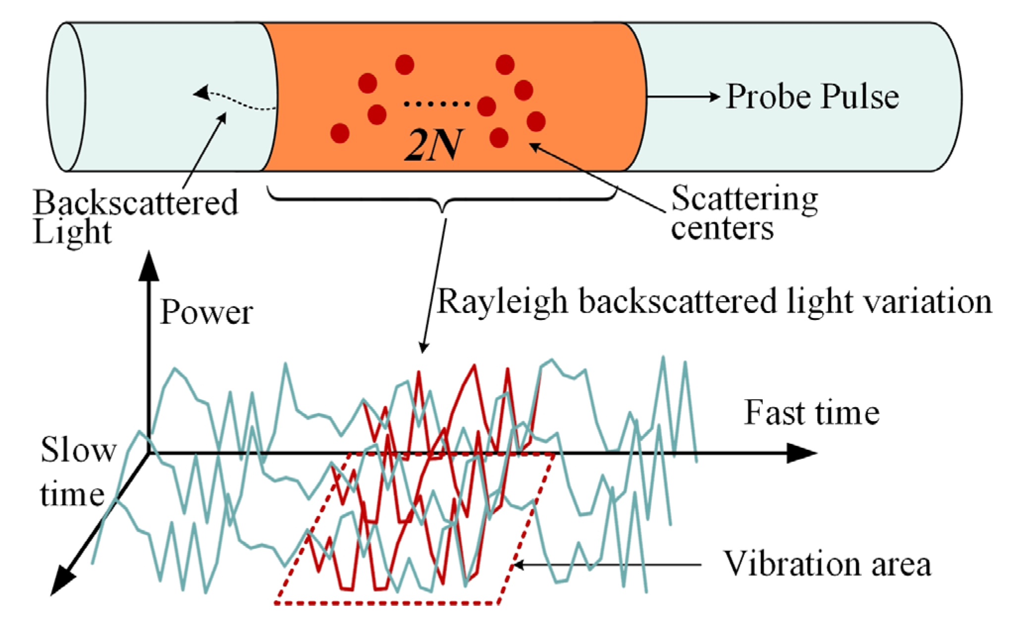
2. Sensing Principle
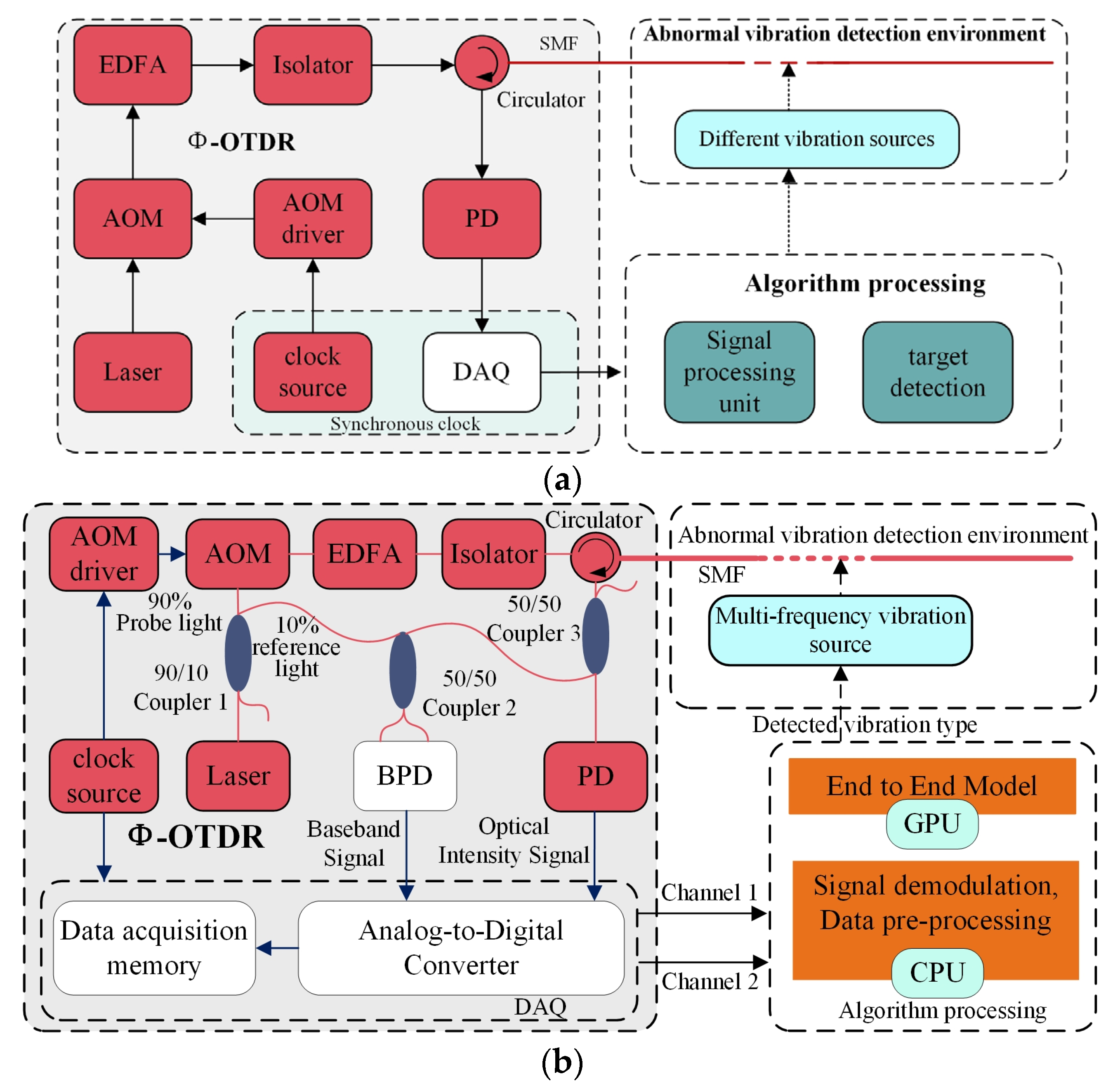
2.1. Φ-OTDR of Direct Detection Combined with Coherent Detection
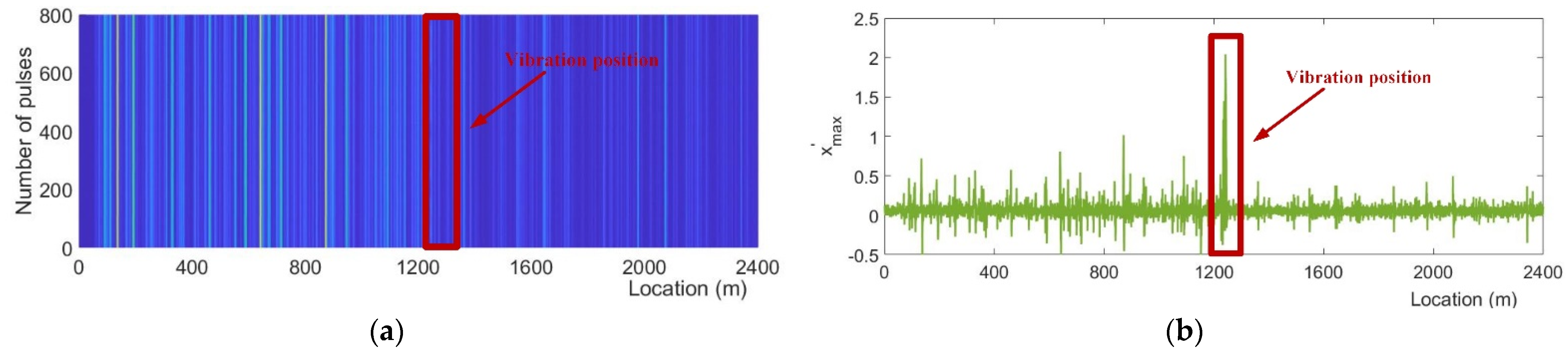
2.2. Raw Data Acquisition Method
3. Methodology
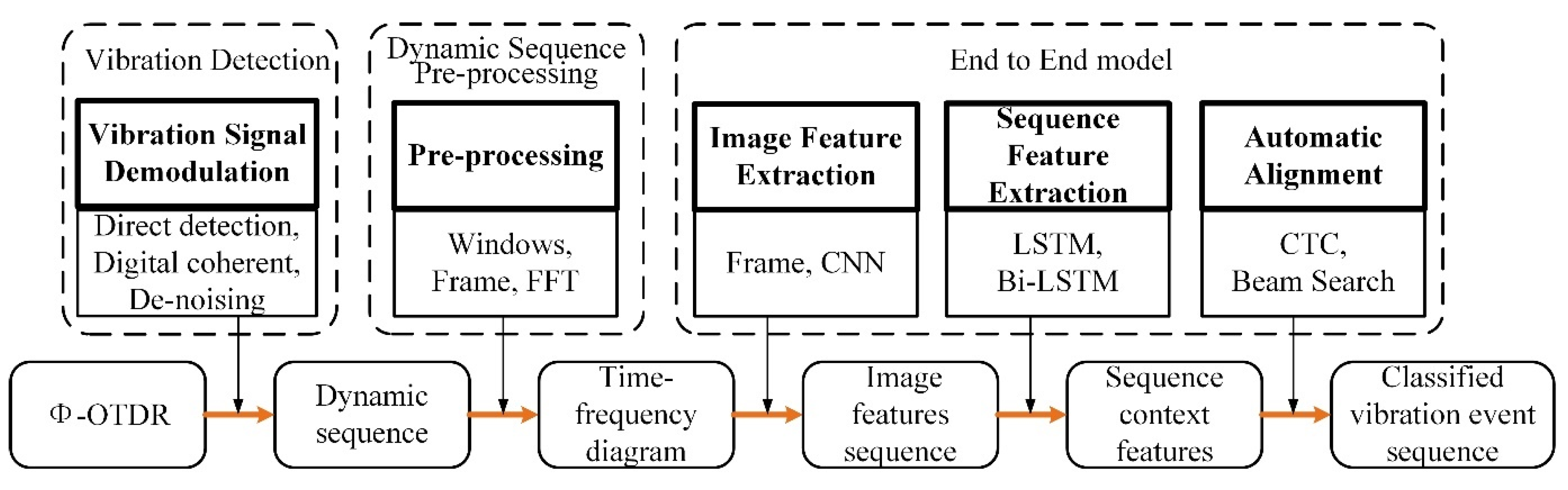
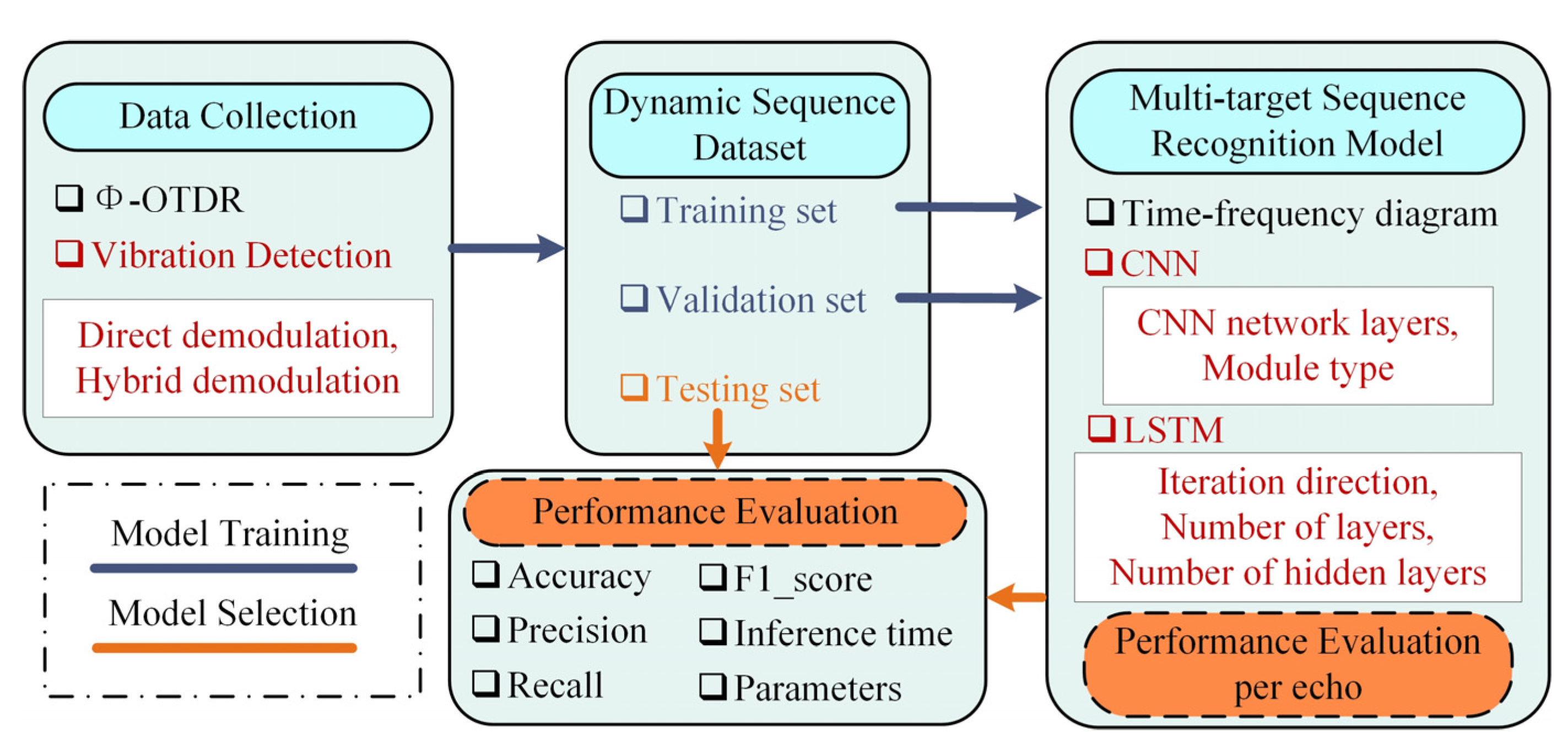
3.1. Proposed Framework
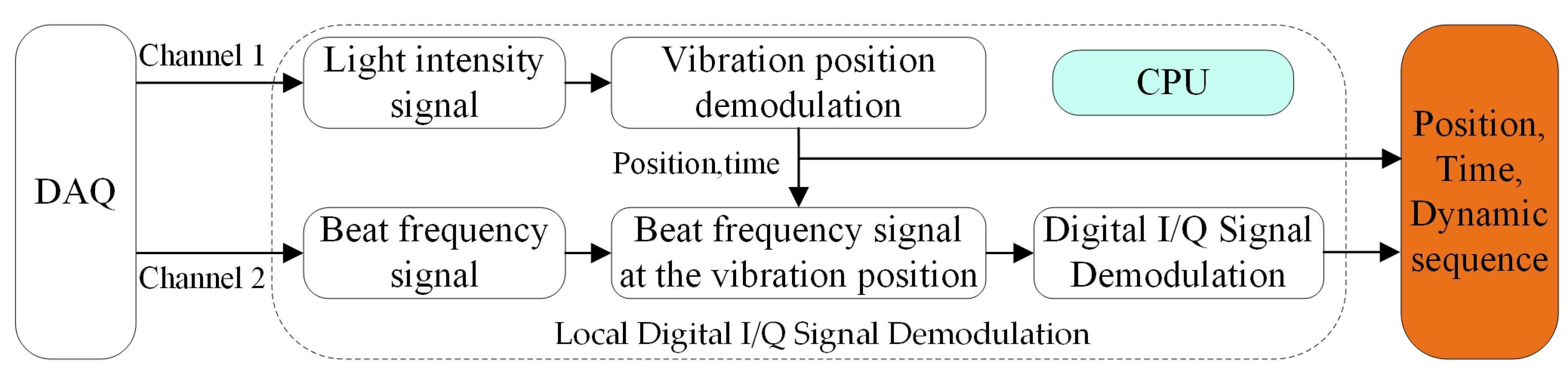
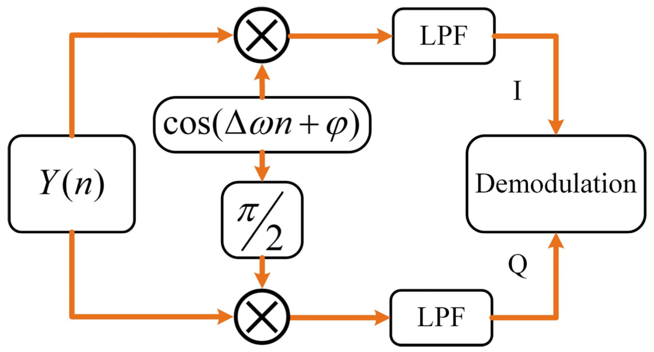
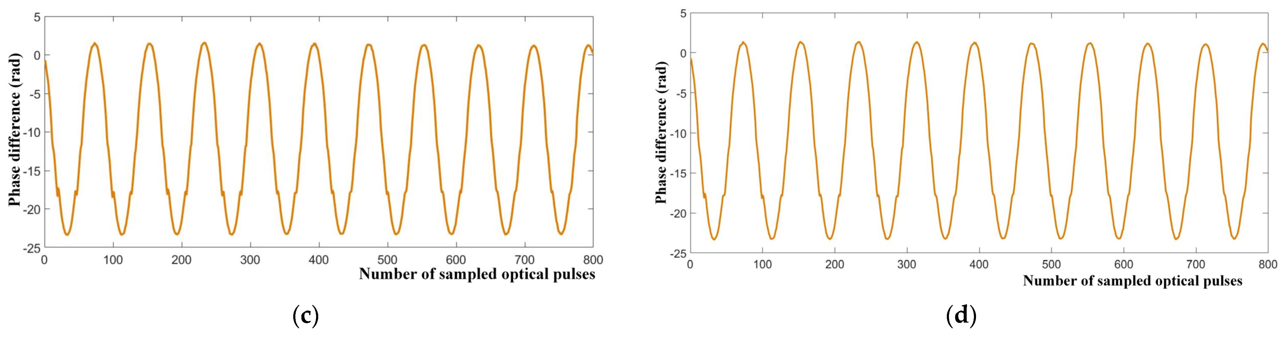
3.2. Local Digital I/Q Signal Demodulation
3.3. Data Time-Frequency Conversion
3.4. Recognition Model
3.4.1. CLSTM and CTC
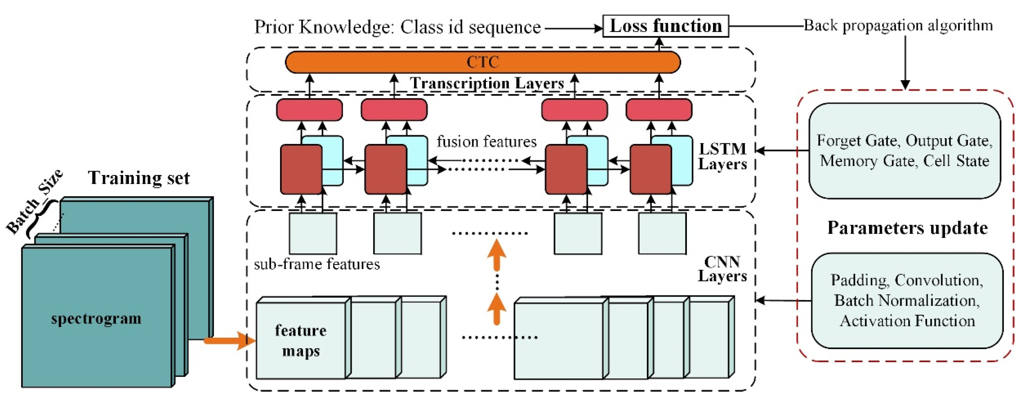
- The CNN layer focuses on extracting image spatial dimensional features, forming feature maps at different scales employing convolution layers, pooling layers, padding, activation functions, etc., thereby extracting high-dimensional features. Since the convolution layer is computed by sliding from left to right on the original image, it has translation invariance. Therefore, each column of the feature map corresponds to a perceptual field at the relevant position on the original image in the same order. The feature map is a sequence of subframe features obtained by sequential operation after dividing the original time–frequency map into frames.
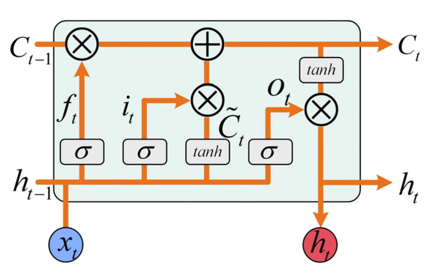
- The LSTM layer extracts the temporal dimensional features of the data. Sequences containing contextual features are extracted by memory gates, forgetting gates, cell states, etc., eventually forming the sequence of labels to be aligned. The depth and length of the extracted sequence features depend on the extraction direction of the LSTM, the number of layers, and the number of hidden layers per LSTM.
- The transcription layer solves the alignment problem between the label and output of the neural network. During the model training, the sequence path probability that matches the label is obtained when the output sequence of LSTM undergoes labeled path search and transform. The smaller the value of this probability, the greater the overall loss of the system.
- Once the system loss value is acquired, the backpropagation algorithm updates the parameters of the algorithm module in the first and second steps. So far, an update iteration operation has been completed. The backpropagation algorithm, including learning rate, learning rate update method, batch size, etc., will affect the training speed and final effect. Therefore, to compare different performance metrics of the models, the parameters of the backpropagation algorithm should be consistent when training different models with multiple iterations until convergence.
3.4.2. Beam Search Decoding Function
4. Experimental Dataset Generation and Preparation
4.1. Data Collection
4.2. Network Construction
4.3. Evaluation Metrics
5. Experimental Procedure
5.1. Experimental Setup
- The processing time of the raw data is compared between two methods of fast hybrid demodulation and global digital I/Q demodulation [13], using piezoelectric ceramics (PZT) as the vibration source.
- The effects of different CNN network structures on the model’s overall performance are discussed. Nine models consisting of CNNs and LSTMs with different structures are used for training and testing, thus addressing the effect of different network structures on model recognition performance.
- The validation set observes the training effect, and the model with satisfactory metrics in Section 4.3 is selected as the final model. The test set is used to analyze various performance metrics. In addition, the performance differences between the proposed CNN network and three classical VGG [44] networks are compared.
- The sequence data collected by Φ-OTDR contain different lengths and different kinds of vibrations. An end-to-end model training method is constructed without using manual forced alignment. The effectiveness of the model for multi-vibration target recognition is verified.
5.2. Fast Hybrid Demodulation Method
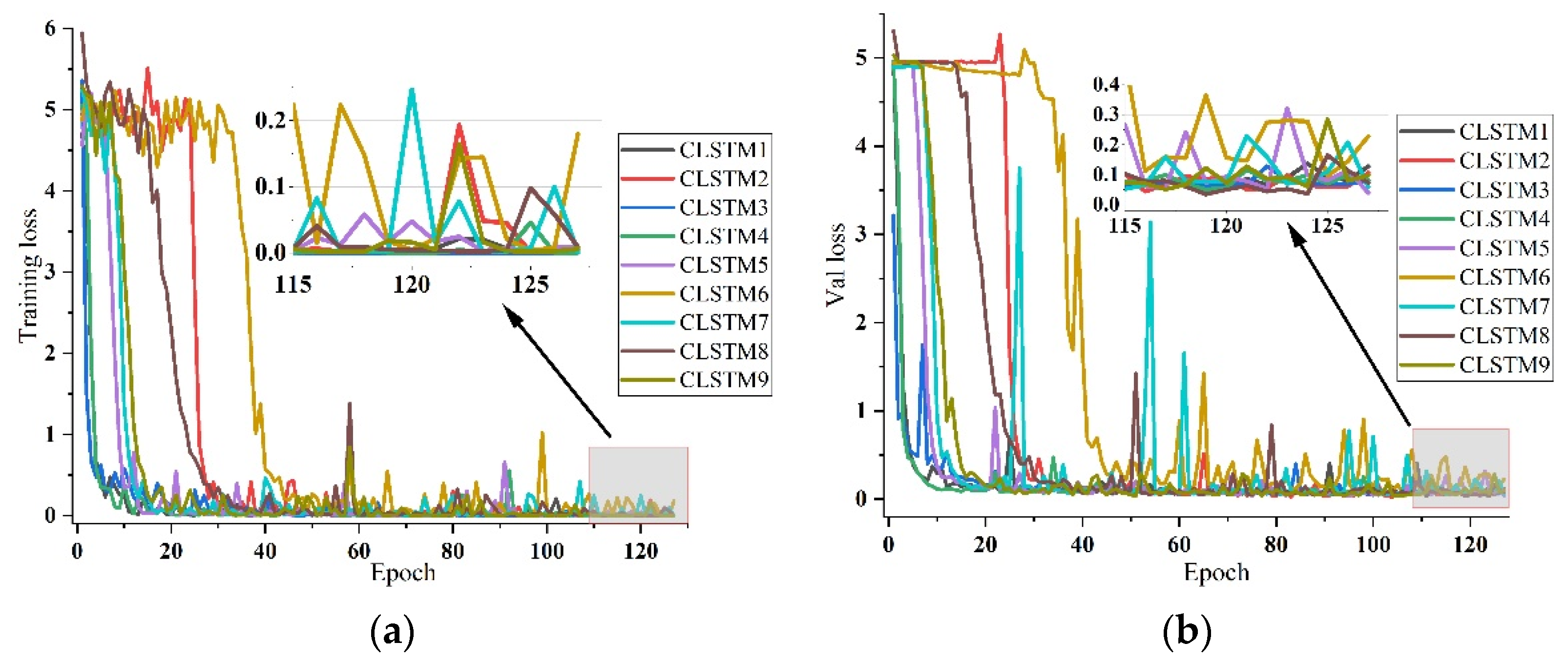
5.3. Network Training
5.4. Models Performance
5.5. Comparison of Models Based on Different CNNs
6. Conclusions and Future Work
Author Contributions
Funding
Data Availability Statement
Acknowledgments
Conflicts of Interest
Abbreviations
| Φ-OTDR | Phase-sensitive Optical Time-domain Reflectometer |
| RBSs | Rayleigh Backscatter Signals |
| CNN | Convolution Neural Network |
| Bi-LSTM | Bidirectional Long Short-term Memory |
| CTC | Connectionist Temporal Classification |
| NARs | Nuisance-alarm Rates |
| L.O. | Local Oscillator |
| EMD | Empirical Mode Decomposition |
| MFCC | Mel-scale Frequency Cepstral Coefficients |
| W.D. | Wavelet Decomposition |
| WPD | Wavelet Packet Decomposition |
| XGBoost | Extreme Gradient Boosting |
| k-NNs | K-nearest Neighbors |
| SVMs | Support Vector Machines |
| GMMs | Gaussian Mixture Models |
| LSTM | Long Short-time memory |
| HMM | Hidden Markov Model |
| AOM | Acoustic-optic Modulator |
| EDFA | Erbium-doped Fiber Amplifier |
| P.D. | Photodetector |
| SMF | Single-mode Fiber |
| DAQ | Data Acquisition Module |
| BPD | Balanced Photodetector |
| STFT | Short-time Fourier Transform |
| FFT | Fast Fourier Transform |
| RNN | Recurrent Neural Networks |
| P.C. | Personal Computer |
| T.P. | True Positive |
| T.N. | True Negative |
| F.P. | False Positive |
| F.N. | False Negative |
| PZT | Piezoelectric Ceramics |
References
- Shang, Y.; Sun, M.; Wang, C.; Yang, J.; Du, Y.; Yi, J.; Zhao, W.; Wang, Y.; Zhao, Y.; Ni, J. Research Progress in Distributed Acoustic Sensing Techniques. Sensors 2022, 22, 6060. [Google Scholar] [CrossRef]
- Muanenda, Y. Recent Advances in Distributed Acoustic Sensing Based on Phase-Sensitive Optical Time Domain Reflectometry. J. Sens. 2018, 2018, 3897873. [Google Scholar] [CrossRef]
- Wang, Z.N.; Zeng, J.J.; Li, J.; Fan, M.Q.; Wu, H.; Peng, F.; Zhang, L.; Zhou, Y.; Rao, Y.J. Ultra-long phase-sensitive OTDR with hybrid distributed amplification. Opt. Lett. 2014, 39, 5866–5869. [Google Scholar] [CrossRef] [PubMed]
- Wang, Y.; Yuan, H.; Liu, X.; Bai, Q.; Zhang, H.; Gao, Y.; Jin, B. A Comprehensive Study of Optical Fiber Acoustic Sensing. IEEE Access 2019, 7, 85821–85837. [Google Scholar] [CrossRef]
- Bao, X.; Zhou, D.P.; Baker, C.; Chen, L. Recent Development in the Distributed Fiber Optic Acoustic and Ultrasonic Detection. J. Light. Technol. 2017, 35, 3256–3267. [Google Scholar] [CrossRef]
- Huang, X.-D.; Zhang, H.-J.; Liu, K.; Liu, T.-G. Fully modelling based intrusion discrimination in optical fiber perimeter security system. Opt. Fiber Technol. 2018, 45, 64–70. [Google Scholar] [CrossRef]
- Tejedor, J.; Macias-Guarasa, J.; Martins, H.; Pastor-Graells, J.; Martin-Lopez, S.; Corredera, P.; Pauw, G.; Smet, F.; Postvoll, W.; Ahlen, C.; et al. Real Field Deployment of a Smart Fiber Optic Surveillance System for Pipeline Integrity Threat Detection: Architectural Issues and Blind Field Test Results. J. Light. Technol. 2017, 36, 1052–1062. [Google Scholar] [CrossRef]
- Meng, H.; Wang, S.; Gao, C.; Liu, F. Research on Recognition Method of Railway Perimeter Intrusions Based on Φ-OTDR Optical Fiber Sensing Technology. IEEE Sens. J. 2021, 21, 9852–9859. [Google Scholar] [CrossRef]
- Yang, N.; Zhao, Y.; Chen, J. Real-Time Φ-OTDR Vibration Event Recognition Based on Image Target Detection. Sensors 2022, 22, 1127. [Google Scholar] [CrossRef]
- Kandamali, D.F.; Cao, X.; Tian, M.; Jin, Z.; Dong, H.; Yu, K. Machine learning methods for identification and classification of events in ϕ-OTDR systems: A review. Appl. Opt. 2022, 61, 2975–2997. [Google Scholar] [CrossRef]
- Lu, Y.L.; Zhu, T.; Chen, L.A.; Bao, X.Y. Distributed Vibration Sensor Based on Coherent Detection of Phase-OTDR. J. Light. Technol. 2010, 28, 3243–3249. [Google Scholar] [CrossRef]
- Izumita, H.; Koyamada, Y.; Furukawa, S.; Sankawa, I. Stochastic amplitude fluctuation in coherent OTDR and a new technique for its reduction by stimulating synchronous optical frequency hopping. J. Light. Technol. 1997, 15, 267–278. [Google Scholar] [CrossRef]
- Pan, Z.; Liang, K.; Ye, Q.; Cai, H.; Qu, R.; Fang, Z. Phase-sensitive OTDR system based on digital coherent detection. In Proceedings of the Asia Communications and Photonics Conference and Exhibition (ACP), Shanghai, China, 13–16 November 2011; pp. 1–6. [Google Scholar]
- Wang, Z.; Lou, S.; Liang, S.; Sheng, X. Multi-class Disturbance Events Recognition Based on EMD and XGBoost in φ-OTDR. IEEE Access 2020, 8, 63551–63558. [Google Scholar] [CrossRef]
- Wang, X.; Liu, Y.; Liang, S.; Zhang, W.; Lou, S. Event identification based on random forest classifier for Φ-OTDR fiber-optic distributed disturbance sensor. Infrared Phys. Technol. 2019, 97, 319–325. [Google Scholar] [CrossRef]
- George, J.; Mary, L.; Riyas, K.S. Vehicle Detection and Classification From Acoustic Signal Using ANN and KNN. In Proceedings of the International Conference on Control Communication and Computing (ICCC), Trivandrum, India, 13–15 December 2013; pp. 436–439. [Google Scholar]
- Wang, Y.; Wang, P.; Ding, K.; Li, H.; Zhang, J.; Liu, X.; Bai, Q.; Wang, D.; Jin, B. Pattern Recognition Using Relevant Vector Machine in Optical Fiber Vibration Sensing System. IEEE Access 2019, 7, 5886–5895. [Google Scholar] [CrossRef]
- Wu, H.; Qian, Y.; Zhang, W.; Tang, C. Feature Extraction and Identification in Distributed Optical-Fiber Vibration Sensing System for Oil Pipeline Safety Monitoring. Photonic Sens. 2017, 7, 305–310. [Google Scholar] [CrossRef] [Green Version]
- Tangudu, R.; Sahu, P.K. Rayleigh Φ-OTDR based DIS system design using hybrid features and machine learning algorithms. Opt. Fiber Technol. 2021, 61, 102405. [Google Scholar] [CrossRef]
- Tejedor, J.; Macias-Guarasa, J.; Martins, H.F.; Martin-Lopez, S.; Gonzalez-Herraez, M. A Multi-Position Approach in a Smart Fiber-Optic Surveillance System for Pipeline Integrity Threat Detection. Electronics 2021, 10, 712. [Google Scholar] [CrossRef]
- Chen, J.; Wu, H.; Liu, X.; Xiao, Y.; Wang, M.; Yang, M.; Rao, Y. A real-time distributed deep learning approach for intelligent event recognition in long distance pipeline monitoring with DOFS. In Proceedings of the 10th International Conference on Cyber-Enabled Distributed Computing and Knowledge Discovery (CyberC), Zhengzhou, China, 18–20 October 2018; pp. 290–296. [Google Scholar]
- Wu, H.; Chen, J.; Liu, X.; Xiao, Y.; Wang, M.; Zheng, Y.; Rao, Y. One-Dimensional CNN-Based Intelligent Recognition of Vibrations in Pipeline Monitoring With DAS. J. Light. Technol. 2019, 37, 4359–4366. [Google Scholar] [CrossRef]
- Xu, C.; Guan, J.; Bao, M.; Lu, J.; Ye, W. Pattern recognition based on time-frequency analysis and convolutional neural networks for vibrational events in φ-OTDR. Opt. Eng. 2018, 57, 016103. [Google Scholar] [CrossRef]
- Cai, M.; Liu, J. Maxout neurons for deep convolutional and LSTM neural networks in speech recognition. Speech Commun. 2016, 77, 53–64. [Google Scholar] [CrossRef]
- Yildirim, O. A novel wavelet sequence based on deep bidirectional LSTM network model for ECG signal classification. Comput. Biol. Med. 2018, 96, 189–202. [Google Scholar] [CrossRef] [PubMed]
- Li, Z.; Zhang, J.; Wang, M.; Zhong, Y.; Peng, F. Fiber distributed acoustic sensing using convolutional long short-term memory network: A field test on high-speed railway intrusion detection. Opt. Express 2020, 28, 2925–2938. [Google Scholar] [CrossRef]
- Yang, Y.; Li, Y.; Zhang, T.; Zhou, Y.; Zhang, H.; Assoc Advancement Artificial, I. Early Safety Warnings for Long-Distance Pipelines: A Distributed Optical Fiber Sensor Machine Learning Approach. In Proceedings of the 35th AAAI Conference on Artificial Intelligence 33rd Conference on Innovative Applications of Artificial Intelligence 11th Symposium on Educational Advances in Artificial Intelligence, Online, 2–9 February 2021; pp. 14991–14999. [Google Scholar]
- Wu, H.; Liu, X.; Xiao, Y.; Rao, Y. A Dynamic Time Sequence Recognition and Knowledge Mining Method Based on the Hidden Markov Models (HMMs) for Pipeline Safety Monitoring With Phi-OTDR. J. Light. Technol. 2019, 37, 4991–5000. [Google Scholar] [CrossRef]
- Wu, H.; Yang, S.; Liu, X.; Xu, C.; Lu, H.; Wang, C.; Qin, K.; Wang, Z.; Rao, Y.; Olaribigbe, A.O. Simultaneous Extraction of Multi-Scale Structural Features and the Sequential Information With an End-To-End mCNN-HMM Combined Model for Fiber Distributed Acoustic Sensor. J. Light. Technol. 2021, 39, 6606–6616. [Google Scholar] [CrossRef]
- Chen, X.; Xu, C. Disturbance pattern recognition based on an ALSTM in a long-distance φ-OTDR sensing system. Microw. Opt. Technol. Lett. 2020, 62, 168–175. [Google Scholar] [CrossRef]
- Pan, Y.; Wen, T.; Ye, W. Time attention analysis method for vibration pattern recognition of distributed optic fiber sensor. Optik 2022, 251, 168127. [Google Scholar] [CrossRef]
- Liu, X.; Wu, H.; Wang, Y.; Tu, Y.; Sun, Y.; Liu, L.; Song, Y.; Wu, Y.; Yan, G. A Fast Accurate Attention-Enhanced ResNet Model for Fiber-Optic Distributed Acoustic Sensor (DAS) Signal Recognition in Complicated Urban Environments. Photonics 2022, 9, 677. [Google Scholar] [CrossRef]
- Lee, W.; Seong, J.J.; Ozlu, B.; Shim, B.S.; Marakhimov, A.; Lee, S. Biosignal Sensors and Deep Learning-Based Speech Recognition: A Review. Sensors 2021, 21, 1399. [Google Scholar] [CrossRef]
- Graves, A.; Fernández, S.; Gomez, F.; Schmidhuber, J. Connectionist temporal classification: Labelling unsegmented sequence data with recurrent neural networks. In Proceedings of the 23rd International Conference on Machine Learning, Pittsburgh, PA, USA, 25–29 June 2006; pp. 369–376. [Google Scholar]
- Shao, Y.; Liu, H.; Peng, P.; Pang, F.; Yu, G.; Chen, Z.; Chen, N.; Wang, T. Distributed Vibration Sensor With Laser Phase-Noise Immunity by Phase-Extraction φ-OTDR. Photonic Sens. 2019, 9, 223–229. [Google Scholar] [CrossRef] [Green Version]
- Wang, Z.; Zhang, L.; Wang, S.; Xue, N.; Peng, F.; Fan, M.; Sun, W.; Qian, X.; Rao, J.; Rao, Y. Coherent Φ-OTDR based on I/Q demodulation and homodyne detection. Opt. Express 2016, 24, 853–858. [Google Scholar] [CrossRef] [PubMed]
- Liang, K.; Pan, Z.; Zhou, J.; Ye, Q.; Cai, H.; Qu, R. Multi-parameter vibration detection system based on phase sensitive optical time domain reflectometer. Chin. J. Lasers 2012, 39, 119–123. [Google Scholar] [CrossRef]
- Taylor, M.G. Phase Estimation Methods for Optical Coherent Detection Using Digital Signal Processing. J. Light. Technol. 2009, 27, 901–914. [Google Scholar] [CrossRef]
- Wu, H.; Yang, M.; Yang, S.; Lu, H.; Wang, C.; Rao, Y. A Novel DAS Signal Recognition Method Based on Spatiotemporal Information Extraction With 1DCNNs-BiLSTM Network. IEEE Access 2020, 8, 119448–119457. [Google Scholar] [CrossRef]
- Ma, X.; Hovy, E.H. End-to-end Sequence Labeling via Bi-directional LSTM-CNNs-CRF. arXiv 2016, arXiv:1603.01354. [Google Scholar]
- Graves, A. Connectionist Temporal Classification. In Supervised Sequence Labelling with Recurrent Neural Networks; Graves, A., Ed.; Springer: Berlin/Heidelberg, Germany, 2012; pp. 61–93. [Google Scholar]
- Bacci, T.; Mattia, S.; Ventura, P. The bounded beam search algorithm for the block relocation problem. Comput. Oper. Res. 2019, 103, 252–264. [Google Scholar] [CrossRef]
- Hu, Z.; Tang, Y.; Yang, S.; Pang, T.; Wu, B.; Zhang, Z.; Sun, M. A new phase demodulation method for φ-OTDR based on coherent detection. In Proceedings of the Proc.SPIE, Online, 8 January 2021; p. 116070M. [Google Scholar] [CrossRef]
- Simonyan, K.; Zisserman, A. Very Deep Convolutional Networks for Large-Scale Image Recognition. arXiv 2014, arXiv:1409.1556. [Google Scholar] [CrossRef]
- He, K.; Zhang, X.; Ren, S.; Sun, J. Deep Residual Learning for Image Recognition. In Proceedings of the 2016 IEEE Conference on Computer Vision and Pattern Recognition (CVPR), Las Vegas, NV, USA, 27–30 June 2016; pp. 770–778. [Google Scholar]
- Yang, N.; Zhao, Y.; Chen, J.; Wang, F. Real-time classification for Φ-OTDR vibration events in the case of small sample size datasets. Opt. Fiber Technol. 2023, 76, 103217. [Google Scholar] [CrossRef]
- Lecun, Y.; Bottou, L.; Bengio, Y.; Haffner, P. Gradient-based learning applied to document recognition. Proc. IEEE 1998, 86, 2278–2324. [Google Scholar] [CrossRef] [Green Version]
- Krizhevsky, A.; Sutskever, I.; Hinton, G. ImageNet Classification with Deep Convolutional Neural Networks. Neural Process. Syst. 2012, 25, 84–90. [Google Scholar] [CrossRef] [Green Version]


| Vibration Source | Included Vibration Frequencies | Lasting Time | Number in Type I Data | Number in Type II Data | Number in Type III Data | Label |
|---|---|---|---|---|---|---|
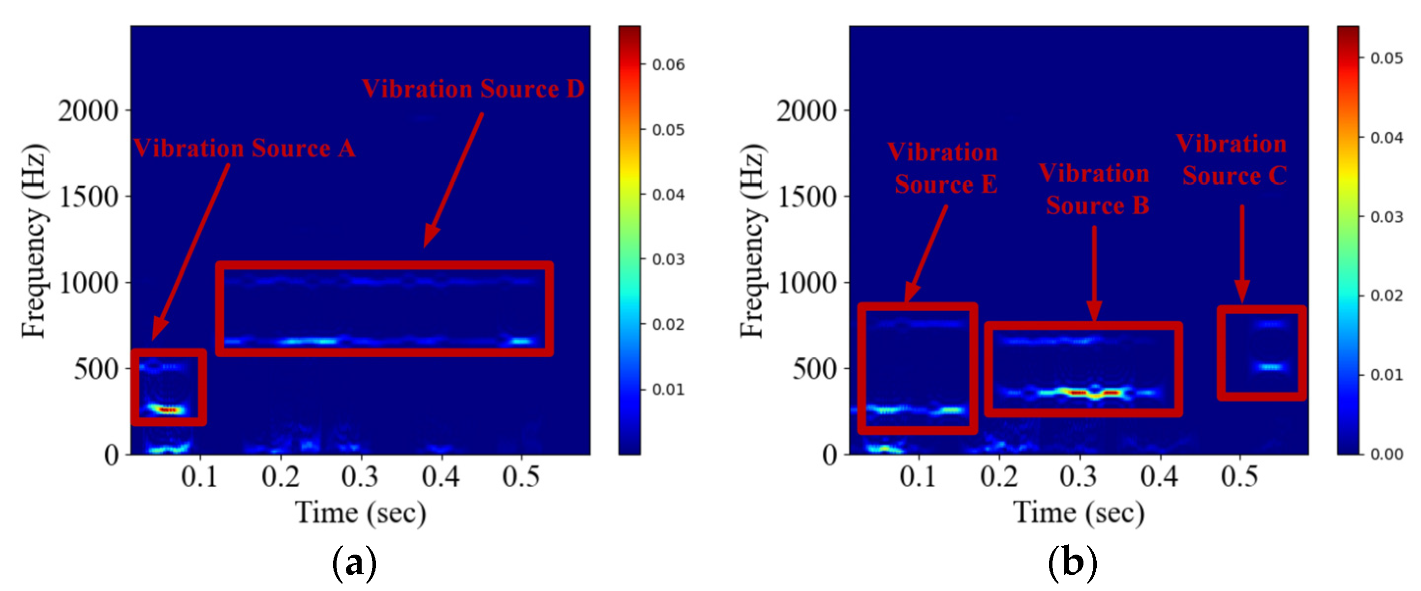
| A | 250 hz, 500 hz | 0.1–0.3 s | 338 | 1366 | 2037 | 1 |
| B | 350 hz, 650 hz | 0.1–0.3 s | 364 | 1383 | 2021 | 2 |
| C | 500 hz, 750 hz | 0.1–0.3 s | 340 | 1361 | 2086 | 3 |
| D | 650 hz, 1000 hz | 0.1–0.3 s | 330 | 1356 | 2046 | 4 |
| E | 250 hz, 750 hz | 0.1–0.3 s | 342 | 1386 | 2079 | 5 |
| Model | CNN | LSTM | Transcription | ||||
|---|---|---|---|---|---|---|---|
| C2 | C3 | C6 | Number of Hidden Layers | Number of Layers | Bi-LSTM | CTC | |
| CLSTM1 | √ | 32 | 2 | √ | √ | ||
| CLSTM2 | √ | 16 | 2 | √ | √ | ||
| CLSTM3 | √ | 64 | 2 | √ | √ | ||
| CLSTM4 | √ | 64 | 1 | √ | √ | ||
| CLSTM5 | √ | 16 | 1 | √ | √ | ||
| CLSTM6 | √ | 64 | 2 | √ | √ | ||
| CLSTM7 | √ | 64 | 2 | √ | √ | ||
| CLSTM8 | √ | 64 | 2 | √ | |||
| CLSTM9 | √ | 16 | 1 | √ | |||
| Model | Type | Precision (%) | Recall (%) | F1 (%) | Accuracy (%) | Number of False Alarms | Number of Missed Alarms | Parameters (M.B.) | Inference (ms) |
|---|---|---|---|---|---|---|---|---|---|
| CLSTM1 | All | 99.34 | 99.18 | 99.26 | 99.18 | 8 | 5 | 21.6 | 2.211 |
| A | 98.62 | 99.44 | 99.03 | ||||||
| B | 99.75 | 99.51 | 99.63 | ||||||
| C | 100 | 99.23 | 99.61 | ||||||
| D | 99.75 | 99.5 | 99.62 | ||||||
| E | 99.75 | 99.5 | 99.62 | ||||||
| CLSTM2 | All | 99.13 | 98.46 | 98.79 | 98.46 | 18 | 5 | 21.3 | 2.206 |
| A | 98.61 | 98.33 | 98.47 | ||||||
| B | 99.51 | 99.75 | 99.63 | ||||||
| C | 99.74 | 98.72 | 99.23 | ||||||
| D | 99.75 | 98.5 | 99.12 | ||||||
| E | 99.23 | 98.23 | 98.73 | ||||||
| CLSTM3 | All | 99.64 | 99.33 | 99.49 | 99.33 | 8 | 2 | 22.3 | 2.204 |
| A | 99.17 | 99.17 | 99.17 | ||||||
| B | 100 | 99.51 | 99.75 | ||||||
| C | 100 | 99.23 | 99.61 | ||||||
| D | 99.75 | 99.5 | 99.62 | ||||||
| E | 99.75 | 99.75 | 99.75 | ||||||
| CLSTM4 | All | 99.49 | 99.18 | 99.33 | 99.18 | 9 | 3 | 21.9 | 2.212 |
| A | 98.62 | 98.89 | 98.75 | ||||||
| B | 100 | 99.75 | 99.88 | ||||||
| C | 100 | 99.23 | 99.61 | ||||||
| D | 100 | 99.5 | 99.75 | ||||||
| E | 99.49 | 99.24 | 99.37 | ||||||
| CLSTM5 | All | 97.47 | 97.51 | 97.48 | 97.51 | 17 | 18 | 21.3 | 2.197 |
| A | 96.48 | 98.89 | 97.67 | ||||||
| B | 98.76 | 98.52 | 98.64 | ||||||
| C | 98.45 | 98.2 | 98.33 | ||||||
| D | 99.75 | 98.5 | 99.12 | ||||||
| E | 98.22 | 97.98 | 98.1 | ||||||
| CLSTM6 | All | 96.04 | 96.71 | 96.37 | 96.71 | 16 | 30 | 1.55 | 2.05 |
| A | 95.1 | 96.94 | 96.01 | ||||||
| B | 98.05 | 99.51 | 98.77 | ||||||
| C | 99.22 | 97.94 | 98.58 | ||||||
| D | 96.56 | 98.5 | 97.52 | ||||||
| E | 98.47 | 97.98 | 98.22 | ||||||
| CLSTM7 | All | 95.12 | 96.99 | 96.04 | 96.99 | 7 | 46 | 4.93 | 2.091 |
| A | 93.67 | 98.61 | 96.08 | ||||||
| B | 97.11 | 99.75 | 98.41 | ||||||
| C | 99.49 | 99.23 | 99.36 | ||||||
| D | 97.78 | 99.25 | 98.51 | ||||||
| E | 98.5 | 99.49 | 98.99 | ||||||
| CLSTM8 | All | 97.93 | 98.42 | 98.17 | 98.42 | 6 | 16 | 21.9 | 2.201 |
| A | 96.99 | 98.33 | 97.66 | ||||||
| B | 99.02 | 99.51 | 99.26 | ||||||
| C | 100 | 98.97 | 99.48 | ||||||
| D | 98.03 | 99.5 | 98.76 | ||||||
| E | 99.5 | 99.75 | 99.62 | ||||||
| CLSTM9 | All | 99.47 | 97.28 | 98.36 | 97.28 | 44 | 1 | 21.3 | 2.196 |
| A | 99.15 | 96.67 | 97.89 | ||||||
| B | 99.8 | 98.76 | 99.25 | ||||||
| C | 99.74 | 97.43 | 98.57 | ||||||
| D | 99.75 | 98 | 98.86 | ||||||
| E | 99.21 | 95.7 | 97.42 |
Disclaimer/Publisher’s Note: The statements, opinions and data contained in all publications are solely those of the individual author(s) and contributor(s) and not of MDPI and/or the editor(s). MDPI and/or the editor(s) disclaim responsibility for any injury to people or property resulting from any ideas, methods, instructions or products referred to in the content. |
© 2023 by the authors. Licensee MDPI, Basel, Switzerland. This article is an open access article distributed under the terms and conditions of the Creative Commons Attribution (CC BY) license (https://creativecommons.org/licenses/by/4.0/).
Share and Cite
Yang, N.; Zhao, Y.; Wang, F.; Chen, J. Using Phase-Sensitive Optical Time Domain Reflectometers to Develop an Alignment-Free End-to-End Multitarget Recognition Model. Electronics 2023, 12, 1617. https://doi.org/10.3390/electronics12071617
Yang N, Zhao Y, Wang F, Chen J. Using Phase-Sensitive Optical Time Domain Reflectometers to Develop an Alignment-Free End-to-End Multitarget Recognition Model. Electronics. 2023; 12(7):1617. https://doi.org/10.3390/electronics12071617
Chicago/Turabian StyleYang, Nachuan, Yongjun Zhao, Fuqiang Wang, and Jinyang Chen. 2023. "Using Phase-Sensitive Optical Time Domain Reflectometers to Develop an Alignment-Free End-to-End Multitarget Recognition Model" Electronics 12, no. 7: 1617. https://doi.org/10.3390/electronics12071617