Supervised Learning Spectrum Sensing Method via Geometric Power Feature

Abstract

In order to improve the spectrum sensing (SS) performance under a low Signal Noise Ratio (SNR), this paper proposes a supervised learning spectrum sensing method based on Geometric Power (GP) feature. The GP is used as the feature vector in the supervised learning spectrum sensing method for training and testing based on the actual captured data set. Experimental results show that the detection performance of the GP-based supervised learning spectrum sensing method is better than that of the Energy Statistics (ES) and Differential Entropy (DE)-based supervised learning spectrum sensing methods.

1. Introduction

With the rapid development of communication technology, 5G beyond and 6G have attracted much attention from researchers. Its characteristics of high speed, low delay and large connection have brought many conveniences to users. At present, 5G is penetrating into various industries and fields of the economic society, becoming a key new infrastructure supporting the digital, networked, and intelligent transformation of the economic society. Although the development of wireless communication technology has solved many practical problems, such as the communication between people and things, and things and things, to meet the needs of mobile medicine, the internet of vehicles, smart homes, industrial control, environmental monitoring and other internet of things applications, the explosive growth of data traffic has followed. Due to the growth of this data traffic, the problem of scarcity of spectrum resources has emerged, and spectrum resources are limited. Therefore, how to improve spectrum efficiency is the focus of current research.

Cognitive Radio (CR) is one of the promising methods to solve the scarcity of spectrum resources. The spectrum can be used as either an authorized frequency band or an unauthorized frequency band; the primary user (PU) is the user who owns the licensed spectrum. These PUs can use the spectrum they own anytime, anywhere, but they do not use the spectrum all the time; when these PUs do not use the licensed spectrum, CR uses the licensed spectrum in an opportunistic way; therefore, CR is also called secondary user (SU). SU can only use the spectrum when the PU is inactive; once the PU uses the spectrum, SU must immediately exit the use and ensure that it will not cause interference to the PU. Therefore, it is critical to timely and accurately detect whether the spectrum is used by the PU. Spectrum sensing (SS) in CR can solve this problem.

SS is one of the key technologies of CR. It can quickly and accurately detect whether the spectrum is used by PU in a complex wireless communication environment, because there are only two cases: firstly, there is no PU, only noise; secondly, both PU and noise exist, so SS can be regarded as a binary classification problem. Traditional SS methods include Energy Detector (ED), Matched Filter Detector (MFD) and Cyclostationary Feature Detector (CFD). Among them, ED [1,2] is the simplest technology, and does not need prior information on PU signals, and has low computational complexity. However, it is vulnerable to noise and multipath fading, resulting in poor detection performance at a low Signal Noise Ratio (SNR). The MFD [3,4] needs prior information on the PU signal, which is difficult to obtain in practice. The CFD [5,6] is insensitive to noise and can distinguish PU signal from noise, and its detection performance is better than that of the ED, but it requires more power consumption and has high computational complexity. It can be seen that there will be many problems in the SS process. In addition to the mentioned noise and multipath fading, there are also problems such as shadows and receiver uncertainty. Machine learning (ML) can solve these problems. Therefore, there is much research that applies ML to SS. ML is divided into supervised learning and unsupervised learning. This paper conducts research based on supervised learning.

Ref. [7], the authors proposed a new SS algorithm based on Support Vector Machines (SVM) [8,9,10], which maps the received signal to the multi-dimensional feature space obtained from the well-known SS statistics and their higher-order combination. The experimental results show that the receiver operating characteristics (ROC) curve of the proposed detector can be better than the classical SS method without knowing the noise variance. Ref. [11], the author selects two ML techniques, SVM and K-Nearest Neighbor (KNN) [12,13,14], in which the detection probability is drawn using SVM and KNN algorithms, with a constant false positive probability. Based on the performance of the false alarm rate, the two ML methods are compared. It can be seen that the KNN algorithm provides a better SS than SVM. Ref. [15], the author proposed a new framework based on Bayesian [16,17,18] ML, which uses the mobility of multiple SUs to simultaneously collect SS data and jointly derive the global spectrum state. Simulation results show that the proposed framework can significantly improve SS performance compared with existing SS technologies. Ref. [19], the author considered three Bayesian SS estimators, weighted Bayesian (WB) estimator, Gaussian Mixture (GM) [20] estimator and a Naive Bayesian (NB) classifier, and compared the results of these technologies with perfect cooperative SS schemes (such as Maximum Ratio Combining (MRC) and AND and OR rules). The experimental results show that the evaluated Bayesian technology provides similar performance to the best MRC technology in the area under the curve (AuC), and has less operation cost for secondary users. Ref. [21], the author assumes that the noise process follows the generalized Gaussian distribution, takes the Differential Entropy (DE) in the received observations as the feature vector, and uses SVM, KNN, Random Forest (RF) [22,23,24] and Logistic Regression (LR) [25,26] to compare the performance. The experimental results show that the method based on DE features is superior to the method based on ES in detection probability, and the proposed technology is particularly useful in the low SNR condition, when the noise distribution has a heavy tail.

On the basis of [21], when the noise distribution has a heavy algebraic tail, the SS based on DE characteristics and the traditional fractional low order statistics (FLOS) can successfully deal with the heavy tail process. However, when the noise distribution has a very heavy algebraic tail, that is, when the algebraic tail constant is close to zero, the processing effect of DE and FLOS will become worse, and geometric power (GP), also known as zero-order statistics [27,28,29,30], is applicable to any process with a number or a light tail, which has been reflected ref. [30]. Ref. [30], the author compares the performance of solving spectrum sensing problems in cognitive radio based on the method of deep learning. However, deep learning not only requires good hardware facilities, but also takes too long to train. These problems do not exist in supervised learning, and this article has found that there has not been any research on using supervised learning for spectrum sensing using GP as input. Based on this, this article proposes a supervised learning spectrum sensing method based on GP features. Firstly, the GP extracted from the observed signal is used as a feature vector, and then it is trained and tested using supervised learning; finally, this method is compared with the supervised learning spectrum sensing method based on ES and DE features. Due to the excessive number of supervised learning methods, this article selects SVM and KNN for simulation experiments using the actual captured data set [31]. Simulation results show that the proposed method has the best perceptual performance, especially at low SNR.

2. Model

2.1. System Model

In general, the spectrum sensing problem is transformed into a binary classification problem, assuming that the signal model is

$$\begin{array}{c}{H}_0:y\left(n\right)=\eta \left(n\right),n=1,\cdots ,N\hfill \\ H_1:y\left(n\right)=x\left(n\right)+\eta \left(n\right)\hfill \end{array}$$

(1)

$H_0$ indicates that PU is not present, i.e., only noise; $H_1$ indicates that the channel has PU and noise, $x\left(n\right)$ is the signal transmitted by PU, $y\left(n\right)$ is the signal received by SU, $\eta \left(n\right)$ is channel noise and N is the number of sampling points.

Different SS algorithms construct statistics T according to different signal characteristics, and then set a threshold value of $\lambda$. Finally, the size of statistics and threshold value $\lambda$ are compared, and whether there is a PU signal to achieve the purpose of detection is determined.

The performance evaluation indicators of spectrum sensing algorithms usually include the following two types:

Probability of detection $P_d$

$$P_d=prob(T>\lambda |H_1)$$

(2)

Probability of false alarm $P_f$

$$P_f=prob(T>\lambda |H_0)$$

(3)

$P_d$ indicates the probability that the signal can be detected correctly under $H_1$ conditions. The larger the value, the smaller the interference and better the data transmission; $P_f$ indicates the probability that there is no signal, but it is judged to be a signal.

2.2. Noise Model

In this paper, we consider CR nodes and run PU transmitters in a specific frequency band to obtain M observations. The characteristic of the generalized Gaussian distribution is that it can describe the probability density, thus realizing the expansion and improvement of data statistics and models. It is actually a reasonable random variable, which can help us reasonably fit the data and effectively predict the condition of the observed values. In addition, its effective application can improve the unified model, reduce the uncertainty and improve the effectiveness of the model. When there is only noise, it is assumed that the samples received by the receiver are independent and uniformly follow the generalized Gaussian distribution, where scale parameter $\alpha >0$, shape parameter $\beta \in (0,2]$, it controls the “shape” of the distribution, that is, the speed of attenuation, and their probability density function $f_X\left(x\right)$ are as follows:

$$f_X\left(x\right)=\frac{1}{2\alpha \mathsf{\Gamma }\left(\frac{1}{\beta }\right)}exp(-\frac{{\left|x\right|}^{\beta }}{\alpha }),x\in \mathbb{R}$$

(4)

When PU and noise exist at the same time, the statistical data of the received signal largely depend on the wireless communication environment and the PU signal itself. However, the research in this paper does not need relevant knowledge about PU signals.

3. Signal Characteristics Analysis

3.1. Energy Statistics (ES)

ES is widely used in spectrum sensing, and its calculation formula is as follows:

$$\widehat{E}=\frac{1}{N}\sum _{k=0}^{N-1}{\left|X_k\right|}^2,k=0,\cdots ,K-1$$

(5)

where N is the number of sampling points and $X_k$ is the output of the kth fast Fourier transform (FFT). When PU signal and noise exist at the same time, the calculated ES value will be greater than the value in the case of noise only. Take the calculated ES as the eigenvector:

$$\mathbf{E}=[{\widehat{E}}_1,{\widehat{E}}_2,\cdots ,{\widehat{E}}_M]$$

(6)

where M is the number of samples.

3.2. Differential Entropy (DE)

Variable X in difference entropy (DE) $h\left(x\right)$ is a continuous random variable defined at $(-\infty ,\infty )$, and its probability density function is $f_X\left(x\right)$. The calculation formula of DE is as follows:

$$h\left(X\right)=-{\int }_{-\infty }^{\infty }{f}_X\left(x\right)log\left(f_X\left(x\right)\right)dx$$

(7)

When there is a PU signal, the estimated DE value will be higher than that in the case of noise only.

In the case of only noise, the estimated value of DE with generalized Gaussian noise is

$$\stackrel{⌢}{h}\left(D\right)=\frac{1}{\beta }-log[\frac{\beta }{2\mathsf{\Gamma }\left(\frac{1}{\beta }\right)}]+\frac{1}{\beta }log[\frac{\beta }{M}\sum _{i=1}^M{\left|D_i-\stackrel{⌢}{D}\right|}^{\beta }]$$

(8)

among them, $\beta \in (0,2]$, $\beta$ controls the noise tail of the generalized Gaussian distribution, $D_i$ is the ith sample, $i=1,\cdots ,M$, and $\stackrel{⌢}{D}$ is the average value of samples in the received sample. The calculation formula is as follows:

$$\stackrel{⌢}{D}=\frac{1}{M}\sum _{i=1}^M{D}_i$$

(9)

Take the calculated DE as the eigenvector:

$$D=[{\widehat{D}}_1,{\widehat{D}}_2,\cdots ,{\widehat{D}}_M]$$

(10)

3.3. Geometric Power (GP)

Traditional power based on second-order statistics describes the strength or power of random signal with mean square value, that is, $K_X^2\left(n\right)=E\left[{\left|X\left(n\right)\right|}^2\right]$ while there is no second-order moment for stable distribution random variable, so the GP solution formula for defining stable distribution random variable $X_i$ is as follows:

$$G_0\left(X_i\right)=exp\left\{E[log\left|X_i\right|]\right\}$$

(11)

where $E[log\left|X\right|]$ represents the logarithmic moment [27].

$$G_P={\left(E{\left|X\right|}^P\right)}^{\frac{1}{P}}$$

(12)

Equation (12) represents the scale parameter of the P-order statistics of random variable $X_i$.

Applying the Lopida Rule:

$$\begin{array}{c}\hfill \begin{array}{cc}\underset{P\to 0}{lim}\frac{logE{\left|X\right|}^P}{P}\hfill & =\underset{P\to 0}{lim}\frac{d}{dp}logE{\left|X\right|}^P\hfill \\ \hfill & =\underset{P\to 0}{lim}\frac{\frac{d}{dp}logE{\left|X\right|}^P}{E{\left|X\right|}^P}\hfill \\ & =\underset{P\to 0}{lim}\frac{E({\left|X\right|}^{P}log\left|X\right|)}{E{\left|X\right|}^P}\hfill \\ \hfill & =Elog\left|X\right|\hfill \end{array}\end{array}$$

(13)

According to Jensen’s inequality:

$$\begin{array}{c}\hfill \begin{array}{cc}{\left(G_0\right)}^P\hfill & =exp(Elog{\left|X\right|}^P)\le Eexp(log{\left|X\right|}^P)\hfill \\ \hfill & =E{\left|X\right|}^P\hfill \\ & ={\left(G_P\right)}^P\hfill \end{array}\end{array}$$

(14)

It can be concluded from Equations (13) and (14) that GP is zero order related to fractional lower order statistics (FLOS), so GP is also called “zero order statistics (ZOS) [27,28]”.

The expected value is replaced by the average value of the samples in the ith sample set, and the geometric power corresponding to the ith sample set is obtained:

$$\begin{array}{cc}\hfill \begin{array}{c}{\stackrel{⌢}{G}}_i\hfill \end{array}& =exp(\frac{1}{N}\sum _{j=1}^{N}log\left|X_{i,j}\right|)\hfill \\ \hfill & =exp(\frac{1}{N}log\prod _{j=1}^N\left|X_{i,j}\right|)\hfill \\ & ={(\prod _{j=1}^N\left|X_{i,j}\right|)}^{\frac{1}{N}},i=1,2,\cdots ,M\hfill \end{array}$$

(15)

where $X_{i,j}$ is the jth sample in the ith sample set.

Take the calculated GP as the eigenvector:

$$G=[{\widehat{G}}_1,{\widehat{G}}_2,\cdots ,{\widehat{G}}_M]$$

(16)

In this paper, GP, ES and DE extracted from the received observations are used as feature vectors, including $E=[{\widehat{E}}_1,{\widehat{E}}_2,\cdots ,{\widehat{E}}_M]$, $D=[{\widehat{D}}_1,{\widehat{D}}_2,\cdots ,{\widehat{D}}_M]$, $G=[{\widehat{G}}_1,{\widehat{G}}_2,\cdots ,{\widehat{G}}_M]$, respectively, and then these feature vectors are trained and tested using machine learning to obtain the corresponding detection performance.

4. Supervised Learning

4.1. Support Vector Machines (SVM)

SVM is commonly used for binary classification. Its principle is to perform classification by finding a hyperplane, which separates the vector representing one type of signal from the vector representing another type of signal, and optimizes the boundary between the two types.

When the kernels are different, the hyperplane equation will also change. In this paper, the linear kernel is used:

$$h_1\left(E\right)={w_1}^T{e}_s+b_1$$

(17)

$$h_2\left(D\right)={w_2}^T{d}_e+b_2$$

(18)

$$h_3\left(G\right)={w_3}^T{g}_p+b_3$$

(19)

among them, $h(·)$ represents the linear kernel, $E$ represents the eigenvector of ES, $D$ represents the eigenvector of DE, $G$ represents the eigenvector of GP, $w$ represents the weight vector, and b represents the deviation amount.

4.2. K-Nearest Neighbors (KNN)

The feature space of the K-nearest neighbor (KNN) model is generally n-dimensional real vector space. The distance between different samples in the feature space reflects the similarity between samples; that is, the closer the “distance” between two samples, the higher the similarity. In general, the definition of distance function $L(x,y)$ needs to meet the four criteria of symmetry, non-negativity and reflexive kernel trigonometric inequality. The definition formula of distance is as follows:

$$L(x,y)={[\sum _{i=1}^n{\left|x_i-y_i\right|}^p]}^{\frac{1}{p}},p\ge 1$$

(20)

Equation (20) is called Minkowski distance. When it meets the above four criteria, the distance metric represented by this equation will be different from the difference of p of the corresponding vector norm.

This paper uses Euclidean distance, that is, $p=2$

$$L(x,y)=\sqrt{\sum _{i=1}^M{(x_i-y_i)}^2}$$

(21)

5. Experimental Simulation and Result Discussion

This paper discusses the performance of the proposed GP feature-based supervised learning SS method, and compares it with peer-to-peer supervised learning algorithms (including SVM and KNN) based on ES and DE features.

The data set used in the simulation is obtained from the experimental device described in [31]. The central frequency of PU is set to 2.48 GHz, the main transmitter adopts differential quadrature phase shift keying modulation, the continuous transmission rate is 500 kbps, and the transmission bandwidth is 1 MHz. The data measurement is carried out in an anechoic chamber with a scanning bandwidth of 4 MHz. The anechoic chamber uses the discrete Fourier transform of 1024 frequency boxes, so the bandwidth of each frequency box is 3.9 kHz. The noise of the generalized Gaussian distribution is added to the given parameters and unit variance as the real data received by the CR node. In 1024 data sets, this article extracts corresponding GP, ES, and DE features from 10,000 data points at specific frequency points in each data set, with 820 data sets for training and 204 data sets for testing.

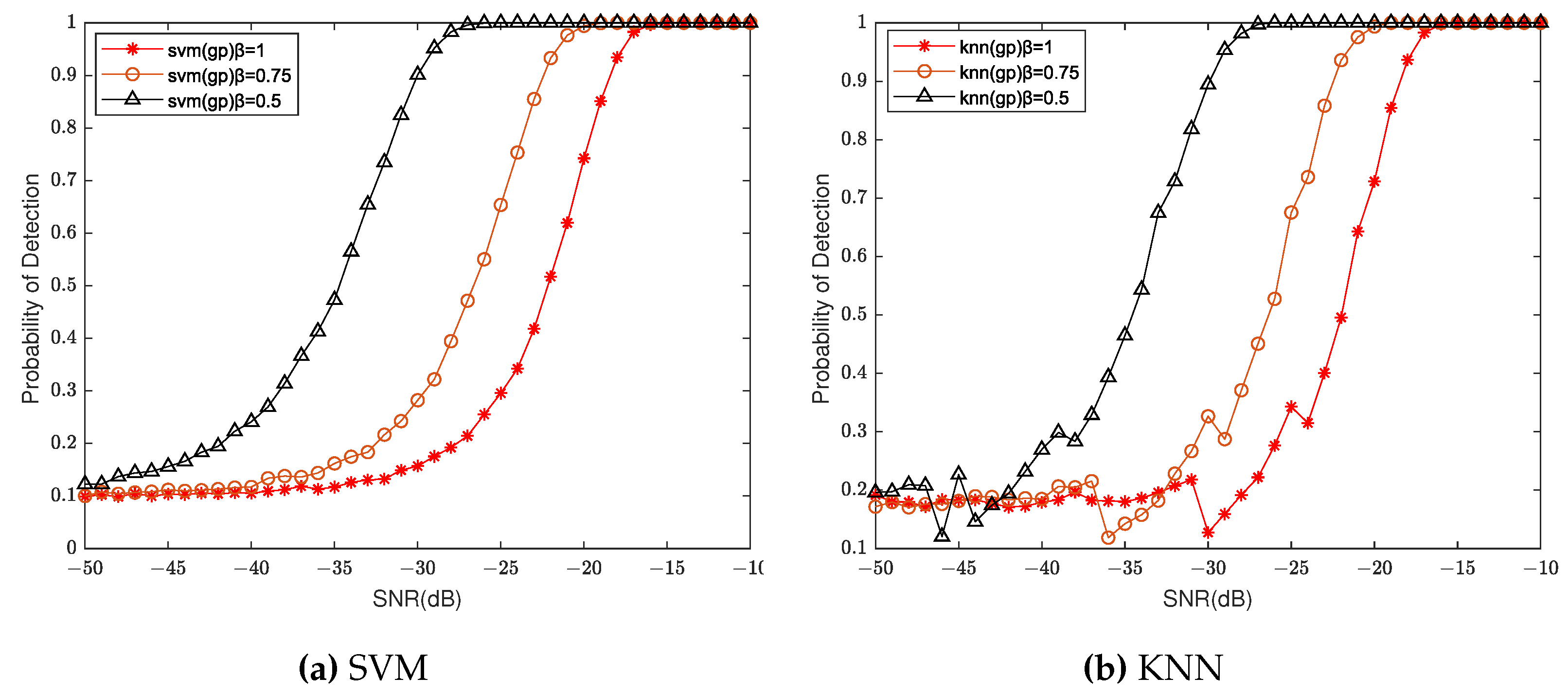
5.1. Selection of Shape Parameter $\beta$

This paper first discusses the shape parameters in noise models $\beta$ Value selection, using geometric power as a feature, and using SVM and KNN for simulation experiments; the results are shown in Figure 1a,b. Among them, Figure 1a is the resulting graph from using SVM, and Figure 1b is the resulting graph from using KNN.

As can be seen from Figure 1a, when $\beta$ = 1, the detection probability reaches 100% at SNR = −15 dB, when $\beta$ = 0.75, the detection probability reaches 100% at SNR = − 19 dB, and when $\beta$ = 0.5, the detection probability reaches 100% at SNR = −25 dB. From Figure 1b, when $\beta$ = 1, the detection probability reaches 100% at SNR = −15 dB, when $\beta$= 0.75, the detection probability reaches 100% at SNR = −19 dB, and when $\beta$ = 0.5, the detection probability reaches 100% at SNR = −26 dB. To sum up, when $\beta$ = 0.5, the performance of the method proposed in this paper is better at low SNR.

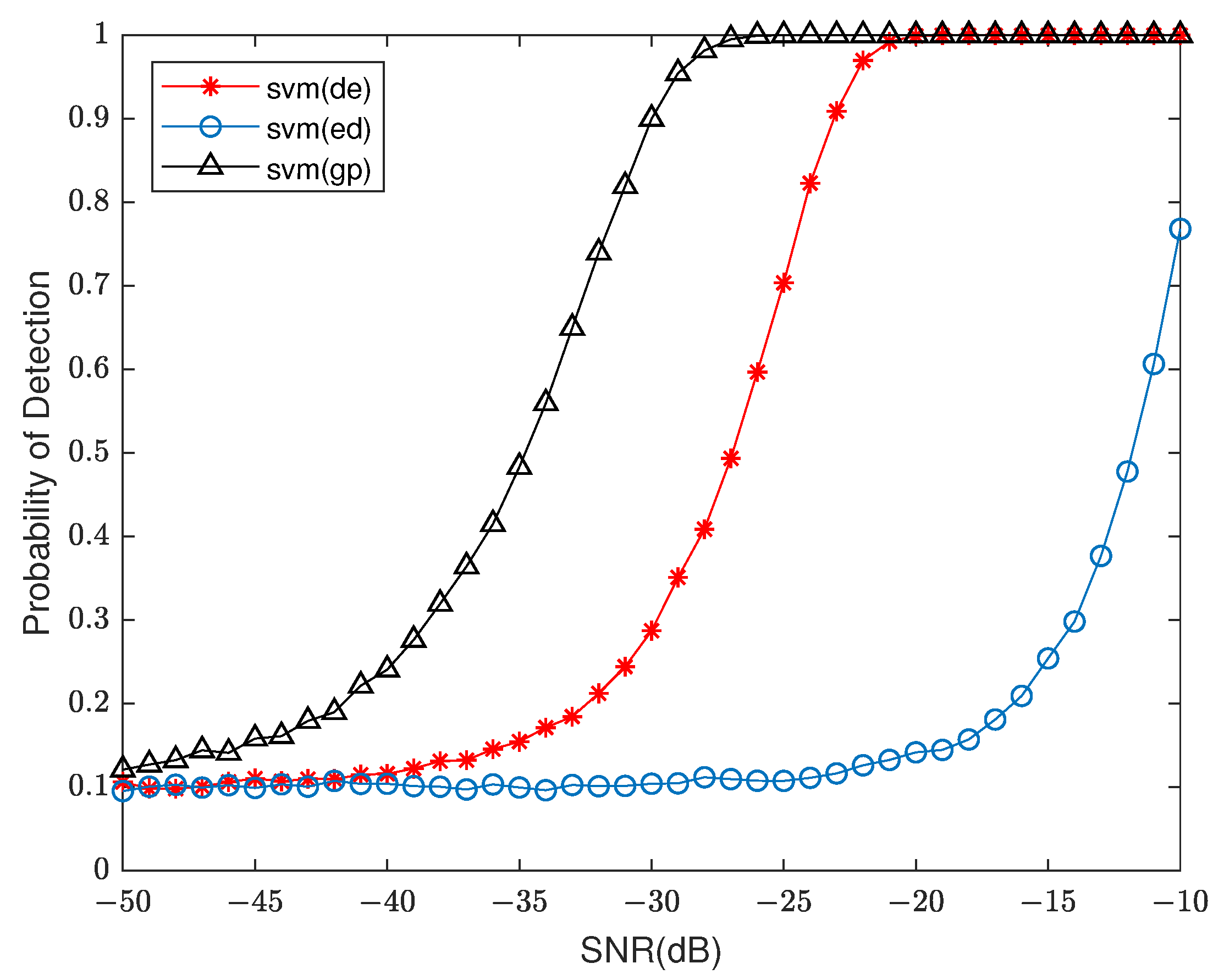
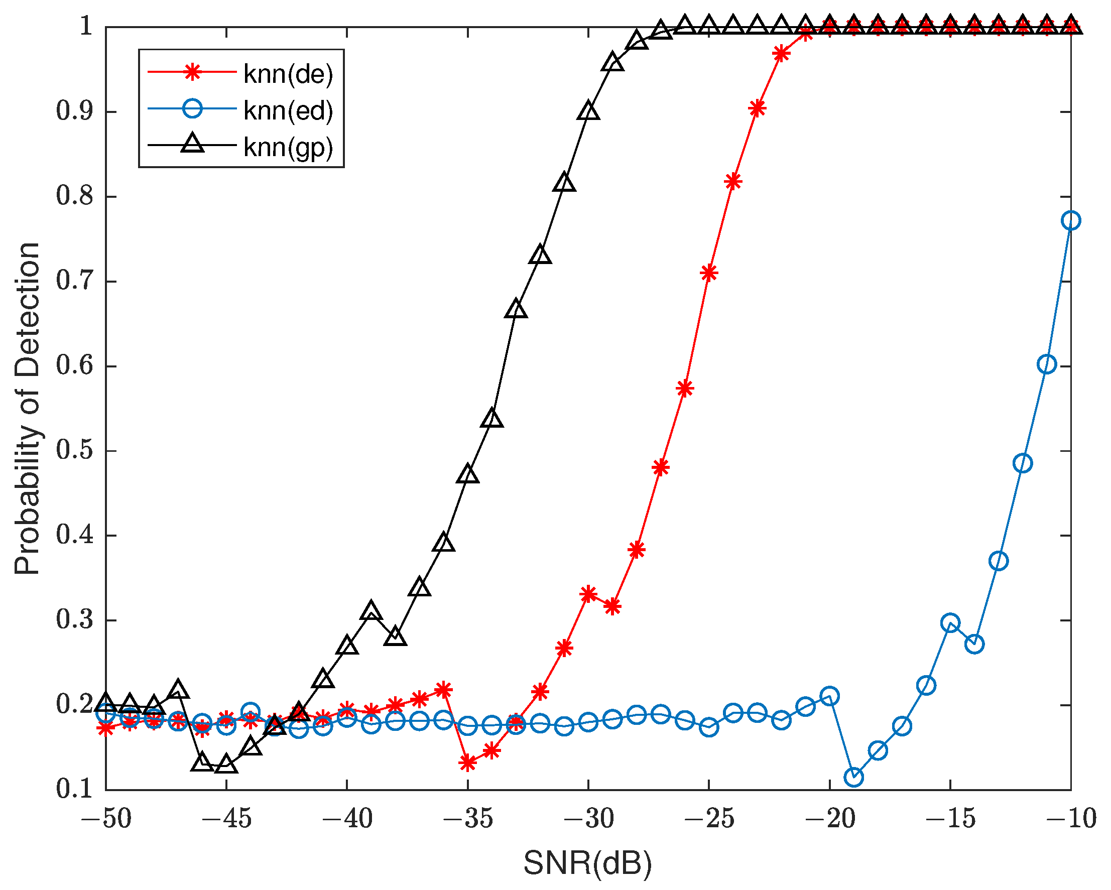
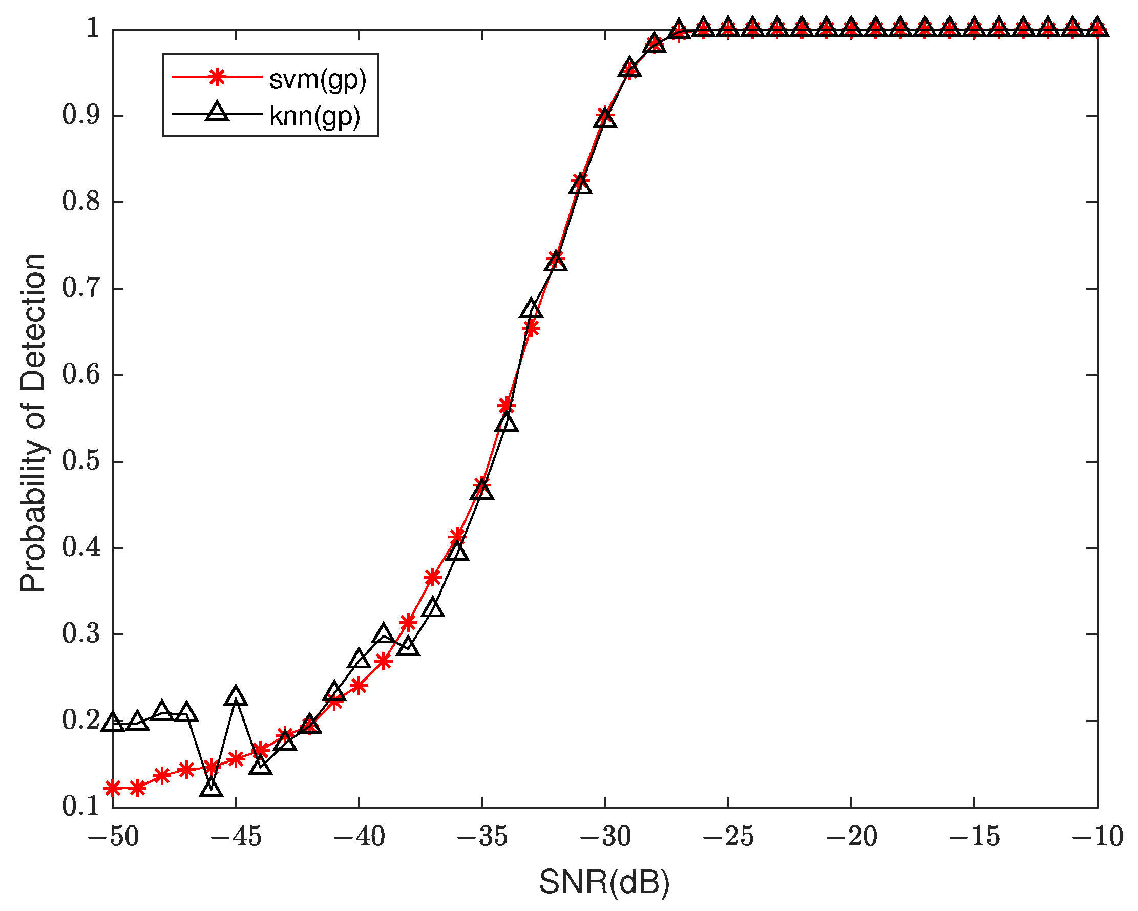
5.2. Performance Comparison

When $\beta$ is 0.5, this paper first compares the area under the receiver curve (AuC) of the SVM spectrum sensing method based on GP, ES and DE, and the KNN spectrum sensing method based on GP, ES and DE. The results are shown in

Table 1. AuC of SVM spectrum sensing method based on GP, ES and DE.

SVM	AuC
GP	1
ES	0.9225
DE	1

and

Table 2. AuC of KNN spectrum sensing method based on GP, ES and DE.

KNN	AuC
GP	1
ES	0.9338
DE	1

.

From the above two tables, it can be seen that the AuC of SVM based on GP and DE and KNN spectrum sensing method is 1. The ES-based KNN spectrum sensing method is superior to the ES-based SVM spectrum sensing method.

Since the AuC of SVM and KNN spectrum sensing methods based on GP and DE are both 1, this paper also considers these three features under low SNR, and the results are shown in Figure 2, Figure 3 and Figure 4.

As can be seen from Figure 2, when the SNR is lower than −25 dB, the detection probability of the SVM spectrum sensing method based on GP features is much higher than that of the SVM spectrum sensing method based on ES features and DE features, and the SVM spectrum sensing method based on GP features can achieve a detection rate close to 1 when the SNR is −27 dB.

As can be seen from Figure 3, when the SNR is lower than −23 dB, the detection probability of the KNN spectrum sensing method based on GP features is much higher than that of the KNN spectrum sensing method based on ES features and DE features, and the KNN spectrum sensing method based on GP features can achieve a detection rate close to 1 when the SNR is −27 dB.

As can be seen from Figure 4, when the SNR is lower than −27 dB, the detection probability of the SVM spectrum sensing method based on GP features and the KNN spectrum sensing method based on GP features are both close to 1. In summary, the performance of the machine learning spectrum sensing algorithm based on GP features proposed in this chapter is better than that of the machine learning spectrum sensing algorithm based on ES features and DE features under low SNR.

6. Results

This paper proposes different supervised learning algorithms that use GP vector as a feature to train cognitive radio SS. Firstly, it is assumed that the samples received by the receiver are independent and uniformly follow the generalized Gaussian distribution, and then the shape parameters of the noise are discussed $\beta$; this paper uses GP as a feature vector, and then uses SVM- and KNN-supervised learning algorithms for training and testing. Simulation results show that when shape parameters $\beta$ = 0.5, the performance of spectrum sensing methods based on GP features is better. Secondly, the performance of spectrum sensing methods based on GP features is compared with those based on ES features and DE features. Based on real captured data sets, experimental simulation results show that the proposed GP feature performs better than ES feature vectors and DE feature vectors, especially when the SNR is low at −27 dB, where the detection probability of the SVM spectrum sensing method based on GP features and the KNN spectrum sensing method based on GP features are both close to 1.

References

1. Nasrallah, A.; Hamza, A.; Messani, A. Robust Spectrum Sensing Using Moving Blocks Energy Detector with Bootstrap. J. Commun. Technol. Electron. 2022, 67, 636–648. [Google Scholar] [CrossRef]
2. Arjoune, Y.; El Mrabet, Z.; El Ghazi, H.; Tamtaoui, A. Spectrum sensing: Enhanced energy detection technique based on noise measurement. In Proceedings of the 2018 IEEE 8th annual computing and communication workshop and conference (CCWC), Las Vegas, NV, USA, 8–10 January 2018; pp. 828–834. [Google Scholar]
3. Salama, U.; Sarker, P.L.; Chakrabarty, A. Enhanced energy detection using matched filter for spectrum sensing in cognitive radio networks. In Proceedings of the 2018 Joint 7th International Conference on Informatics, Electronics & Vision (ICIEV) and 2018 2nd International Conference on Imaging, Vision & Pattern Recognition (icIVPR), virtual, 19–25 June 2018; pp. 185–190. [Google Scholar]
4. Salahdine, F.; El Ghazi, H.; Kaabouch, N.; Fihri, W.F. Matched filter detection with dynamic threshold for cognitive radio networks. In Proceedings of the 2015 international conference on wireless networks and mobile communications (WINCOM), Marrakech, Morocco, 20–23 October 2015; pp. 1–6. [Google Scholar]
5. Shrestha, R.; Telgote, S.S. A short sensing-time cyclostationary feature detection based spectrum sensor for cognitive radio network. In Proceedings of the 2020 IEEE International Symposium on Circuits and Systems (ISCAS), Sevilla, Spain, 10–21 October 2020; pp. 1–5. [Google Scholar]
6. Sherbin, K.; Sindhu, V. Cyclostationary feature detection for spectrum sensing in cognitive radio network. In Proceedings of the 2019 International Conference on Intelligent Computing and Control Systems (ICCS), Madurai, India, 15–17 May 2019; pp. 1250–1254. [Google Scholar]
7. Coluccia, A.; Fascista, A.; Ricci, G. Spectrum sensing by higher-order SVM-based detection. In Proceedings of the 2019 27th European Signal Processing Conference (EUSIPCO), Coruña, Spain, 2–6 September 2019; pp. 1–5. [Google Scholar]
8. Bao, J.; Nie, J.; Liu, C.; Jiang, B.; Zhu, F.; He, J. Improved blind spectrum sensing by covariance matrix Cholesky decomposition and RBF-SVM decision classification at low SNRs. IEEE Access 2019, 7, 97117–97129. [Google Scholar] [CrossRef]
9. Saber, M.; El Rharras, A.; Saadane, R.; Aroussi, H.K.; Wahbi, M. Artificial neural networks, support vector machine and energy detection for spectrum sensing based on real signals. Int. J. Commun. Netw. Inf. Secur. 2019, 11, 52–60. [Google Scholar] [CrossRef]
10. Jan, S.U.; Vu, V.H.; Koo, I.S. Performance analysis of support vector machine-based classifier for spectrum sensing in cognitive radio networks. In Proceedings of the 2018 International Conference on Cyber-Enabled Distributed Computing and Knowledge Discovery (CyberC), Zhengzhou, China, 18–20 October 2018; pp. 385–3854. [Google Scholar]
11. Tamilselvi, T.; Rajendran, V. Comparative Study of SVM and KNN Machine Learning Algorithm for Spectrum Sensing in Cognitive Radio. In Intelligent Communication Technologies and Virtual Mobile Networks: Proceedings of ICICV 2022; Springer: Berlin/Heidelberg, Germany, 2022; pp. 517–527. [Google Scholar]
12. Saber, M.; El Rharras, A.; Saadane, R.; Kharraz, A.H.; Chehri, A. An optimized spectrum sensing implementation based on SVM, KNN and TREE algorithms. In Proceedings of the 2019 15th International Conference on Signal-Image Technology & Internet-Based Systems (SITIS), Sorrento, Italy, 26–29 November 2019; pp. 383–389. [Google Scholar]
13. An, C.; Zhang, D.; Yuan, C.; Li, L.; Zhao, X.; Geng, S.; Zheng, W.; Shao, W. Spectrum sensing based on KNN algorithm for 230 MHz power private networks. In Proceedings of the 2018 12th International Symposium on Antennas, Propagation and EM Theory (ISAPE), Hangzhou, China, 3–6 December 2018; pp. 1–4. [Google Scholar]
14. Inamdar, M.A.; Kumaraswamy, H. Accurate primary user emulation attack (PUEA) detection in cognitive radio network using KNN and ANN classifier. In Proceedings of the 2020 4th International Conference on Trends in Electronics and Informatics (ICOEI)(48184), Tirunelveli, India, 15–17 June 2020; pp. 490–495. [Google Scholar]
15. Xu, Y.; Cheng, P.; Chen, Z.; Li, Y.; Vucetic, B. Mobile collaborative spectrum sensing for heterogeneous networks: A Bayesian machine learning approach. IEEE Trans. Signal Process. 2018, 66, 5634–5647. [Google Scholar] [CrossRef]
16. Liu, X.; Sun, C.; Zhou, M.; Wu, C.; Peng, B.; Li, P. Reinforcement learning-based multislot double-threshold spectrum sensing with Bayesian fusion for industrial big spectrum data. IEEE Trans. Ind. Inform. 2020, 17, 3391–3400. [Google Scholar] [CrossRef]
17. Liu, X.; Zhang, X.; Ding, H.; Peng, B. Intelligent clustering cooperative spectrum sensing based on Bayesian learning for cognitive radio network. Hoc Netw. 2019, 94, 101968. [Google Scholar] [CrossRef]
18. Arjoune, Y.; Kaabouch, N. Wideband spectrum sensing: A Bayesian compressive sensing approach. Sensors 2018, 18, 1839. [Google Scholar] [CrossRef] [PubMed] [Green Version]
19. Tavares, C.H.A.; Abrão, T. Bayesian estimators for cooperative spectrum sensing in cognitive radio networks. In Proceedings of the 2017 IEEE URUCON, Montevideo, Uruguay, 23–25 October 2017; pp. 1–4. [Google Scholar]
20. Zhao, X.; Li, F. Sparse Bayesian compressed spectrum sensing under Gaussian mixture noise. IEEE Trans. Veh. Technol. 2018, 67, 6087–6097. [Google Scholar] [CrossRef]
21. Saravanan, P.; Chandra, S.S.; Upadhye, A.; Gurugopinath, S. A supervised learning approach for differential entropy feature-based spectrum sensing. In Proceedings of the 2021 Sixth International Conference on Wireless Communications, Signal Processing and Networking (WiSPNET), Chennai, India, 25–27 March 2021; pp. 395–399. [Google Scholar]
22. Valadão, M.D.; Amoedo, D.; Costa, A.; Carvalho, C.; Sabino, W. Deep cooperative spectrum sensing based on residual neural network using feature extraction and random forest classifier. Sensors 2021, 21, 7146. [Google Scholar] [CrossRef] [PubMed]
23. Tan, C.; Chen, J.; Chen, S.; Li, C.; Liu, H.; Zheng, M. Combination Spectrum Sensing Algorithm for Wireless Sensor Network Based on Random Forest. In Proceedings of the 2022 10th International Conference on Intelligent Computing and Wireless Optical Communications (ICWOC), Chongqing, China, 10–12 June 2022; pp. 1–5. [Google Scholar]
24. Gao, Z.; Wang, X. Spectrum Sensing Algorithm Based on Random Forest in Dynamic Fading Channel. In Advances in Simulation and Process Modelling: Proceedings of the 2nd International Symposium on Simulation and Process Modelling (ISSPM 2020) 2; Springer: Singapore, 2021; pp. 39–46. [Google Scholar]
25. Liu, J.; Mu, H.; Vakil, A.; Ewing, R.; Shen, X.; Blasch, E.; Li, J. Human occupancy detection via passive cognitive radio. Sensors 2020, 20, 4248. [Google Scholar] [CrossRef] [PubMed]
26. Wajhal, G.; Dehalwar, V.; Jha, A.; Ogura, K.; Kolhe, M.L. Proactive Handoff of Secondary User in Cognitive Radio Network Using Machine Learning Techniques. In Proceedings of International Conference on Intelligent Computing, Information and Control Systems, Madurai, India, 3–15 May 2020; Pandian, A.P., Palanisamy, R., Ntalianis, K., Eds.; ICICCS: Singapore, 2021; pp. 9–22. [Google Scholar]
27. Chen, J.; Chen, H. Parameter estimation method of alpha stable distribution based on zero order statistics. Electron. Inf. Countermeas. Technol. 2017, 32, 6. [Google Scholar]
28. Gonzalez, J.G.; Griffith, D.W.; Arce, G.R. Zero-order statistics: A signal processing framework for very impulsive processes. In Proceedings of the IEEE Signal Processing Workshop on Higher-Order Statistics, Banff, AB, Canada, 21–23 July 1997; pp. 254–258. [Google Scholar]
29. Gurugopinath, S.; Muralishankar, R. Geometric power detector for spectrum sensing under symmetric alpha stable noise. Electron. Lett. 2018, 54, 1284–1286. [Google Scholar] [CrossRef]
30. Chandra, S.S.; Upadhye, A.; Saravanan, P.; Gurugopinath, S.; Muralishankar, R. Deep Neural Network Architectures for Spectrum Sensing Using Signal Processing Features. In Proceedings of the 2021 IEEE International Conference on Distributed Computing, VLSI, Electrical Circuits and Robotics (DISCOVER), Shivamogga, India, 19–20 November 2021; pp. 129–134. [Google Scholar]
31. Gurugopinath, S.; Muralishankar, R.; Shankar, H.N. Robust spectrum sensing based on spectral flatness measure. Electron. Lett. 2017, 53, 890–892. [Google Scholar] [CrossRef]
Figure 1. Based on different machine learning pairs β value selection.
Electronics 12 01616 g001
Figure 2. Performance comparison of SVM spectrum sensing methods based on GP, ES and DE.
Electronics 12 01616 g002
Figure 3. Performance comparison of KNN spectrum sensing methods based on GP, ES and DE.
Electronics 12 01616 g003
Figure 4. Performance comparison of GP-based SVM and KNN spectrum sensing methods.
Electronics 12 01616 g004