Towards Convergence in Federated Learning via Non-IID Analysis in a Distributed Solar Energy Grid

Abstract

Federated Learning (FL) is an effective framework for a distributed system that constructs a powerful global deep learning model, which diminishes the local bias and accommodates the successful aggregation of locally trained models with heterogeneous datasets. However, when local datasets have the non-IID attribute, the optimization metric tends to diverge or show unstable convergence in the trajectory space. This paper delves into building a global model for the distributed Smart Grid environment, with regionally cumulated three solar energy datasets from January 2017 to August 2021 in a decentralized power grid in South Korea via FL. This distributed energy network involves local properties and physical distance between the regions, which raises a fundamental question of “Will time-serially curated non-IID local features be effective in constructing a global regression model?”. This paper probes this question by leveraging FL and conducts the theoretically viable non-IID case-by-case convergence analysis, providing the interpretation of the embedded temporal non-IID features and application on real-world data. Moreover, most of the FL studies predetermine the global update period, which lacks applicability when adapting FL in actual practice. As FL is a cumulative-basis structure, the update term is a crucial factor that needs to be carefully selected. This paper articulates this problem and explores the effective update period via multiple experiments on the 4.5 years of solar energy dataset, and to the best of my knowledge, this is the first literature that presents the optimal update period in the FL regression in an energy domain.

1. Introduction

The distributed environment is a practical setting that independently curates local datasets, which reflect the intrinsic attributes and properties that may vary in each local environment. In such settings, Federated Learning (FL) [1] is known to be a suitable architecture that accommodates the successful aggregation of heterogeneously trained local models that mirrors its local environments. It reduces regional bias and enhances generalizability without transmitting all the local datasets into one primary server, which guarantees local data privacy. However, when periodically accumulated local datasets are not independent and identically distributed (non-IID), the global model in FL tends to diverge without obtaining a smooth convergence trajectory in the learning space. This condition typically occurs in the real-world system and has been suggested as a significant issue that needs to be solved for further implementation of FL to achieve successful utilization.

One of the distributed system domains that show an interest in utilizing FL is Smart Grid. Smart Grid is a decentralized-oriented power grid network architecture that adaptively accommodates the best utilization of electricity resources that consist of multiple agents (prosumers), synchronously producing and consuming energy by forecasting the future energy amounts. As a vast dataset volume is being generated in the Smart Grid environment in real-time (e.g., multimodal sensors), and the conventional process such as transmitting raw dataset, combining, storing, and preprocessing into an ideal format, then training the model inside a global server is a heavy process, and is not systematically suitable in such decentralized environment. Moreover, the energy dataset involves valuable information, such as correlation to national security or companies’ and users’ privacy; its security must be preserved. FL provides a breakthrough to those problems, offering solutions to efficiently operate the existing processes and to preserve data privacy. Smart Grid is a paradigm that operates in a parallel fashion; it optimizes the allocation of available resources (i.e., Distributed Energy Resources; DER) and energy inside the discrete geographical area (e.g., Micro-Grid), which is an ideal environment for applying FL, as shown in Figure 1.

However, to effectively adapt FL in a Smart Grid, it encounters several realistic hindrances. Establishing a high-performance deep learning forecasting model is crucial, which requires data engineering and extracting salient features that directly and deviously affect the target variable. The primary issues of FL in a dispersed energy grid to predict the DER can be summarized as follows.

Non-deterministic attribute—Obfuscates the future strategy: The FL with an objective function being classification has been widely studied concerning convergence analyses [2] and applications [3,4] since it assumes that the existing label types are predefined, which makes comparatively a straightforward setting. However, regression is a relatively arduous task compared to classification since the expected output vector is mostly continuous within the time domain, which must be accompanied by an assumption that the local datasets share similar distribution-wise statistical features to extract information. Such stochastic attribute increases the efforts of fine-tuning the single global model in FL to build a successful management system and hinders the stable convergence of the iteratively aggregated global model.

Data-level limitation—non-IID in real practice: In actual practice, most datasets frequently encompass the skewed, biased distribution with non-IID attributes. The target distribution range and observed time domain properties may vary in each local dataset. Additionally, data loss may incur triggered by equipment malfunctions, low bandwidth, etc., which will unbalance the dataset volume at the local level. These unexpected anomalies enhance the difficulty of maintaining the identical setting in the system, which will dilute the similarity of the input features.

Algorithmic-level limitation—Unstable convergence: FL is essentially an iteratively cumulated process that non-linearly trains the parameters and linearly aggregates the selected locals. Thus, a poorly trained local model and ineffective selection among the network will trigger the global model to suffer unstable convergence that generates a biased model, or it may incur divergence (i.e., client drift [5]) in the worst case.

This paper adopts the FL framework in a non-IID scenario that accommodates the effective convergence optimization in the non-IID local dataset while predicting the quantitative energy utilization (e.g., energy production, consumption to target) for constructing future response strategies. This work conducts a theoretical convergence analysis while inserting a biased dataset and discovering the preeminent periodical global updates. The presented empirical experiment results validate this claim via training a real-setting solar power energy generation dataset from January 2017 to August 2021 in three disparate locations in South Korea [6]. Furthermore, we explore the periodical training effect and update the central global model in the real-world environment, presenting the optimal update period that converges, returning the lowest loss value among the suggested candidates of the update scheme. To the best of my knowledge, this is the initial study that offers the effective update period selection of the regression-based task in FL, also investigating the time-series non-IID property analysis with practically viable cases. The summary of contributions of this research is as follows:

• This work defines the viable case-by-case scenarios of the locally collected non-IID dataset. It suggests a quantification scheme of the non-IID degree in a regression-based FL network with both local and global perspectives. To the best of my knowledge, this is the first study that covers the domain of local non-IID attributes in the FL regression task.
• This work suggests theoretical convergence analysis in FL regression optimization based on the quantitative degree of IID and non-IID attributes at the local training dataset, proposing a practical training approach to enhance the convergence rate of the global model.
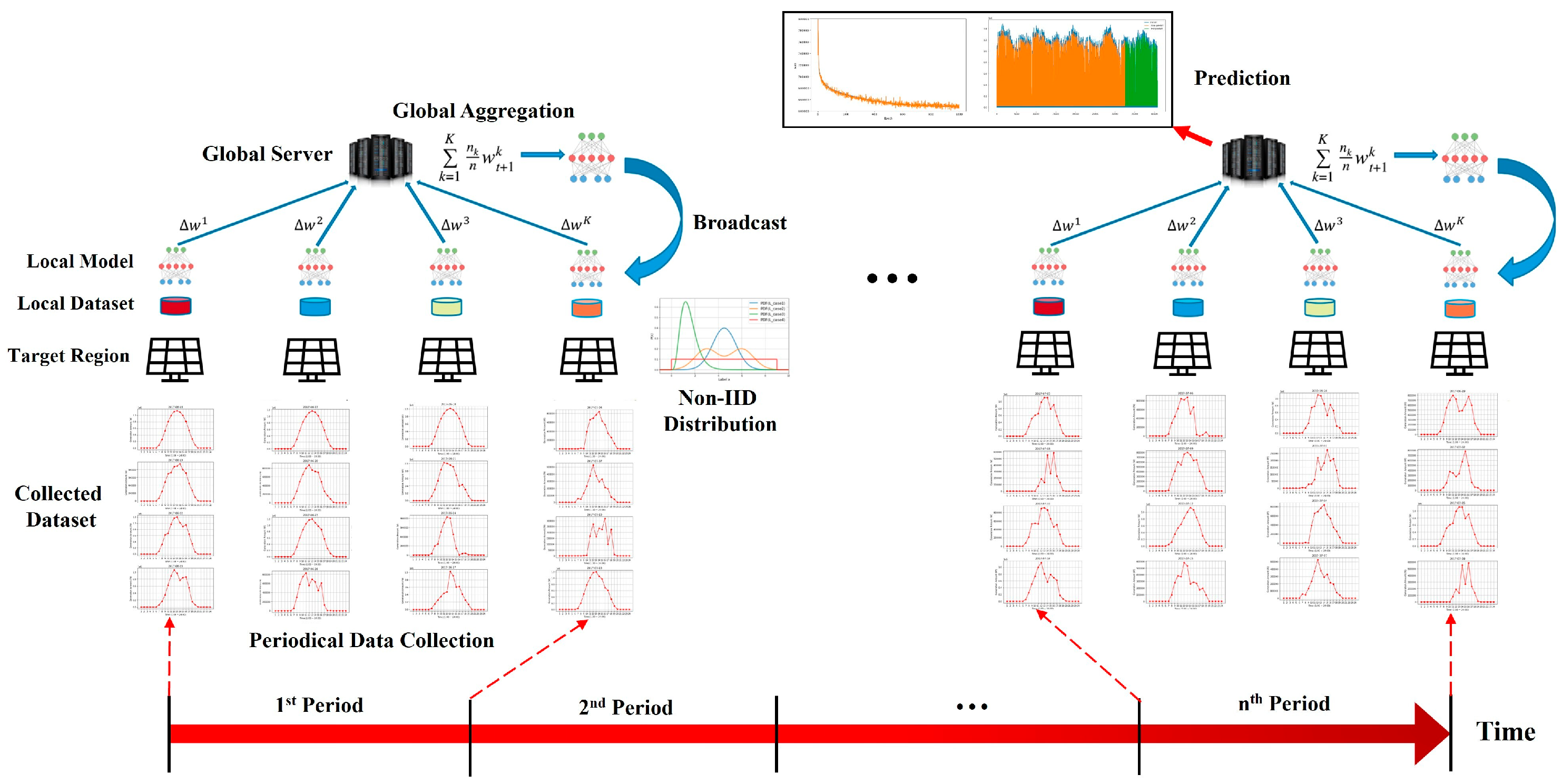
• This work validates the suggested analysis through multiple experiments in the FL model with the distributed solar energy generation dataset in specific regions of South Korea within the period of January 2017 to August 2021 to empirically vindicate the usability and performance of the suggested FL regression and update periods in future applications in the Smart Grid system.

The contents covered in this paper are organized as follows: Section 2 illustrates the milestones concerning FL in energy prediction in the Power Grid environment and previous footprints of non-IID-related FL studies. Section 3 covers the preliminaries of FL and explicates the non-IID and IID attributes in FL regression, which defines the feasible non-IID cases suited for actual practice. Section 4 illustrates the estimated dataset’s non-IID degree and performs convergence analysis of the FL regression with multiple experiments. Finally, Section 5 concludes this study by offering insights and core elements that need to be covered in future studies.

2. Related Works

FL is a diversely implemented architecture for optimizing the power grid system for pragmatic energy usage [7,8] via collaboration with geographically dispersed AI models. Diverse studies were suggested to design a cost-effective structure in such an energy-grid system, analyzing the challenges and issues from multiple perspectives, such as resource allocation, convergence analysis [3,4], and network cost [9]. Zhai et al. [10] applied the FL algorithm in dynamic network bandwidth settings in edge computing in the power grid. Liu et al. [11] brought the concept of horizontal and vertical FL and implemented those concepts into predicting power consumption. They merged the encryption algorithm while transferring information between the local and the server to ensure privacy. Since privacy concerns are a significant issue in the Smart Grid, studies were conducted to mitigate the vulnerability through FL. Wen et al. [12] proposed the energy theft anomaly detection model in the FL network and compared its detection performance with other models. Zhao et al. [13] designed the anomaly detection scheme in the solar farm data to prevent the injection attack. FL-based blockchain technologies were also studied in the smart environment [14]. Al-Quraan et al. [15] presented a cost-efficient measure concerning communication and computation by processing the collected data in a Smart Grid environment. Additionally, Wang et al. [16] analyzed the consumer’s characteristic dataset, leveraged privacy-enhanced PCA to diminish the features, and applied it to the ANN for target attribute identification. Zhao et al. [17] applied differential privacy into FL to enhance the security of local-level LSTM that predicts the energy consumption of individual households’ datasets. Similarly, privacy-preserving FL was recently studied in energy grid environments, most of them to achieve the secure aggregation of local information at the global level [18,19]. Petrangeli et al. [20] performed energy forecasting on the distributed residential household areas with an energy dataset measured from multimeters, and they empirically showed the trade-off between privacy and performance. Likewise, previous studies that dealt with FL in specific energy grid settings were mainly on the rudimentary steps of adapting the FL toward achieving classification-based tasks.

The primary objective of FL in a Smart Grid is to aggregate the local information and collaboratively produce the constructive measure by predicting the target unit, such as energy demand (i.e., base load and peak load) and energy production (i.e., renewable energy). To investigate related works, Taïk et al. [21] conducted individual short-term load forecasting by FL in distantly proximate houses in the state of Texas, USA, and applied a real-world dataset to build a robust prediction model in FL. Zhang et al. [22] introduced an efficient data-management FL system trained through deep reinforcement learning in IIoT settings. Moreover, FL was widely implemented in energy demand learning (EDL) domains, and Saputra et al. [23] adopted EDL in the distributed data of electric vehicles, predicting the energy demand in Dundee city, UK. Huang et al. [24] propounded FL in parking service estimation and resource allocation via LSTM and applied Stackelberg game theory and reinforcement learning to enhance the utility of the parking lot operations. FL scheme is also used in non-intrusive load monitoring (NILM) in the power grid and technology in a distributed environment to analyze the power consumption data for constructive usage [25,26]. These initial approaches proposed the novelty and proof that FL is indeed an effective structure to be applied in the power system. On the other hand, most of these studies do not involve practical usage, as the FedAvg tends to be vulnerable to classification problems while non-IID data are fed into the model.

When it comes to non-IID, although in a different field compared to this study, multiple literature were presented to minimize the effect of a non-IID using the clustering algorithm. Nightingale et al. [27] suggested energy forecasting schemes using multiple clusters to categorize the clients with similar attributes using K-means and scored lower RMSE and MAPE compared to conventional FL, which offers that sorted models with spatial information perform better. Similarly, Brigg et al. [28] leveraged the clustering method in FL (FL + HC; hierarchical clustering) and built an energy forecasting model with a non-IID dataset. This manuscript lies in a similar context in dealing with a non-IID dataset. Although studies [29,30] exist that explore the classification task in non-IID settings, existing works did not thoroughly investigate the intrinsic properties of the serially curated non-IID dataset, which fundamentally limits the utilization of further regression-oriented application domains. This work offers a theoretical analysis of possible case-by-case non-IID scenarios and applies the analysis in a real-life setting to validate the claim. Moreover, this work provides intuitive explanations by exploring interior features that it involves non-IID attributes to essentially comprehend the time-serial statistics.

FL is a cumulative process that iteratively updates the global model after local-level aggregation, and the optimal update period is considered critical to building a high-performance global model. This period agenda has recently been intensely studied by Yan et al. [31] with various criteria, including batch size, weight decay, learning rate annealing, etc. Most of the conventional FL studies pre-set the update period, which is a significant matter when designing an applicable system in the Smart Grid scenario. This work articulates this issue and utilizes 4.5 years-period dataset to demonstrate the training impact of a multiple global update period. Furthermore, this work offers the optimal updating term based on empirical analysis that realizes the best performance.

3. FL Regression: Trained with Non-IID and IID

3.1. Federated Learning

FL has become a successful framework as the locally curated dataset volume has vastly increased [32], and transmitting, preprocessing, managing, and training those datasets only in a centralized system undisputedly requires high cost. Moreover, more distributed systems are adopting a decentralized collaboration since locally acquired heterogeneous information is valuable for discovering local and global knowledge and reducing bias. Furthermore, FL preserves the privacy and security of the edge dataset. It iteratively builds a powerful global model by aggregating the local clients [33], which is generalizable, locally and time-wise agnostic, not overfitted to a particular distribution. In general, when the target incorporates robust spatiotemporal features, this is a well-suited task in FL, where it productively aggregates the embedded features. However, when the target domain must embrace diversity, FL may not be the best alternative, and preserving those heterogeneities may be appropriate. Nevertheless, one particular setting will plausibly trigger the overfitting; thus, contemplating the locals that share similar features is helpful. Therefore, examining the target environment is critical to evaluate the potential effect of FL. Our Smart Grid is considered befitting since clients share high-level features, and acquiring those subtly different distributions helps avoid overfitting and construct a global model. The basic formula of the global model in FL (FedAvg [1]) is indicated as follows Equations (1)–(5).

$${\mathbb{G}}^{\left(T\right)}\ni {\mathbb{W}}^{\left(T\right)}:=\frac{1}{n\left(R\right)}{{\displaystyle \sum }}_{i=R\left[0\right]}^{n\left(R\right)}{W}_i^{\left(T,t\right)}$$

(1)

$$W_i^{\left(T,t\right)}:=\left\{{{\displaystyle \cup }}_{\forall j}{w}_{i,j}^{\left(T,t\right)},{{\displaystyle \cup }}_{\forall j}{b}_{i,j}^{\left(T,t\right)}\right\}$$

(2)

$$R:=\left\{l|1\le l \le n\left({{\displaystyle \cup }}_{\forall i}i\right)\right\}s.t.R \subseteq {{\displaystyle \cup }}_{\forall i}i$$

(3)

$$\begin{gathered} W_i^{\left(T,t+1\right)}=W_i^{\left(T,t\right)}-\eta \frac{\partial \mathbb{L}\left(h_i^{\left(T,t\right)},y_i\right)}{\partial W_i^{\left(T,t\right)}} \\ s.t.\underset{t\to \mathsf{𝕥}}{\lim }\left(\underset{\forall i}{\min }\mathbb{L}\left(f\left(D_i^{\left(T\right)},W_i^{\left(T,t\right)}\right),y_i^{\left(T\right)}\right)\right):W_i^{\left(T,1\right)}\to W_i^{\left(T,\mathsf{𝕥}\right)} \end{gathered}$$

(4)

$$f^{\left(T\right)}\left(u_{\forall j}^{\left(t\right)}\cdot x_{\forall j}^{\left(t\right)}+w_{\forall j}^{\left(t\right)}\cdot h_{\forall j}^{\left(t\right)}+b_{\forall j}^{\left(t\right)}\right)\to h^{\left(T,t\right)}\in {ℝ}^d$$

(5)

Note that the variables and parameters used in this study are listed in Notations. The individual model $M_i(\cdot )$ are identical regression model types, and $n\left({{\displaystyle \cup }}_{\forall k}{\ell }_{\left(\exists i,k\right)}\right)=c\in \mathbb{N}$ since (1) is a pairwise and elementwise computation inside a matrix form, where $n\left(W_{\forall i}\right)=\widehat{c}\in \mathbb{N}$ and when $\left(n\left(W_{\forall i}\right)\ne n\left(W_{\forall i^{\prime }}\right)\right)or\left(n\left({{\displaystyle \cup }}_{\forall k}{\ell }_{\left(\exists i,k\right)}\right)\ne n\left({{\displaystyle \cup }}_{\forall k}{\ell }_{\left(\exists i^{\prime },k\right)}\right)\right)\nrightarrow \underset{T\to \mathbb{T}}{\lim }\left(\underset{t\to \mathsf{𝕥}}{\lim }\left(\underset{\forall i}{\min }\mathbb{L}\left(h_i^{\left(T,t\right)},y\right)\right)\right)$ [2,5].

3.2. Non-IID Cases in Regression-Based FL

This section defines the non-IID cases in the regression-based FL environment, which globally modifies the global model with two perspectives. First, this section describes the FL cases with the data-structural view in Section 3.2.1 and construes the FL-structural standpoint in Section 3.2.2.

3.2.1. Non-IID Cases with a Structural View

The feasible cases are as follows:

• Case A. $n\left(D_{\left(\exists i,train\right)}^{\left(T,t\right)}\right)\ne n\left(D_{\left(\exists i^{\prime },train\right)}^{\left(T,t\right)}\right) s.t. i\ne i^{\prime } and D_i=\left({{\displaystyle \cup }}_{\forall j}{x}_j,{{\displaystyle \cup }}_{\forall j}{y}_j\right)$.
• Case B. $\psi \left(\mathbb{D}\left({{\displaystyle \cup }}_{\forall j}{y}_{\left(\exists i,j\right)}\right),\mathbb{D}\left({{\displaystyle \cup }}_{\forall j}{y}_{\left(\exists i^{\prime },j\right)}\right)\right)\gg 0s.t.i\ne i^{\prime }andn\left({{\displaystyle \cup }}_{\forall j}{y}_{\left(\exists i,j\right)}\right)=n\left({{\displaystyle \cup }}_{\forall j}{y}_{\left(\exists i^{\prime },j\right)}\right)$ in (5).
• Case C. $\frac{1}{{{\displaystyle \cup }}_{\forall j}1}{\displaystyle \sum }_{\forall j}\left(\delta \left(y_{\left(i,j\right)},y_{\left(i^{\prime },j\right)}\right)\right)\gg 0$.

Case A indicates the different amount of data in each local while identical epoch (i.e., global/local). Assorted environmental factors such as low bandwidth and faulty sensors may incur data loss in identical sampling rate and data acquisition frequency. Case B illustrates the different distribution of ${{\displaystyle \cup }}_{\forall j}{y}_j$ in $\exists i$ and $\exists i^{\prime }$, representing the condition of $y_i$. This value can be utilized to measure the quantitative quality of a particular local dataset to serve as the standard for selecting $M_{l\in R}$. It implements the Kullback–Leibler divergence in (6) to compute the density difference of $y_{\left(i,i^{\prime }\right)}$, and determine as non-IID when it satisfies Case B. Depending on the environmental characteristic, $\mathbb{D}\left({{\displaystyle \cup }}_{\forall j}{y}_{\left(\exists i,j\right)}\right)$ may have unique distribution, such as $y_i~N\left(\mu \left(y_{\forall i}\right),{\sigma }^2\left(y_{\forall i}\right)\right)$, $y_i~Gamma\left(\alpha ,\beta \right)$, etc., and when $\sigma \left({{\displaystyle \cup }}_{\forall i}\mathbb{D}\left({{\displaystyle \cup }}_{\forall j}{y}_{\left(\exists i,j\right)}\right)\right)\approx 0$, the most frequent $\mathbb{D}\left({{\displaystyle \cup }}_{\forall j}{y}_{\left(\exists i,j\right)}\right)$ becomes the ground truth. The left term in Case C shows the time-dependent distribution difference $\delta \left(y_i,y_{i^{\prime }}\right)$ in (7). On the other hand, Case B does not consider the time-series attribute, which may incur the risk of unstable convergence while training the local models. Typically, time-series datasets embed the temporal-domain features that must be utilized to obtain (4). Thus, this is designated as another metric for the non-IID dataset.

$$\psi \left(\mathbb{D}\left(\underset{\forall j}{{\displaystyle \cup }}{y}_{\left(\exists i,j\right)}\right),\mathbb{D}\left(\underset{\forall j}{{\displaystyle \cup }}{y}_{\left(\exists i^{\prime },j\right)}\right)\right):={\displaystyle \sum }_{\forall j}\mathbb{D}\left(\underset{\forall j}{{\displaystyle \cup }}{y}_{\left(\exists i,j\right)}\right)\log \frac{\mathbb{D}\left({{\displaystyle \cup }}_{\forall j}{y}_{\left(\exists i,j\right)}\right)}{\mathbb{D}\left({{\displaystyle \cup }}_{\forall j}{y}_{\left(\exists i^{\prime },j\right)}\right)}$$

(6)

$\delta \left(y_i,y_{i^{\prime }}\right):=y_i-y_{i^{\prime }}inelementwise\mathrm{and}pairwisefashion$

$$s.t. y_i=\underset{\forall j}{{\displaystyle \cup }}{y}_{\left(i,j\right)},y_{i^{\prime }}=\underset{\forall j}{{\displaystyle \cup }}{y}_{\left(i^{\prime },j\right)}$$

(7)

3.2.2. Non-IID Cases in FL-Structural View

The training in FL has three primary levels: individual local client-level training with $t$ epoch, aggregation of every local client in a single global $T$ communication round, and training with $T\to \mathbb{T}$ global round. The categorization of the cases via three levels is as follows: $\left(\exists i,\exists T\right)\prec \left(\forall i,\exists T\right)\prec \left(\forall i,\forall T\right)$.

• Case 1. $\left(M_{\exists i}^{\left(\exists T\right)},M_{\exists i^{\prime }}^{\left(\exists T\right)}\right)\to case A or B or C$.
• Case 2. $\left(M_{\exists i}^{\left(\exists T\right)},M_{\exists i^{\prime }}^{\left(\exists T\right)}\right)\nrightarrow case A or B or C$.
• Case 3. $\left(M_{\forall i}^{\left(\exists T\right)},M_{\forall i}^{\left(\exists T^{\prime }\right)}\right)\to case A or B or C$.
• Case 4. $\left(M_{\forall i}^{\left(\exists T\right)},M_{\forall i}^{\left(\exists T^{\prime }\right)}\right)\nrightarrow case A or B or C$.
• Case 5. $\left(M_{\forall i}^{\left(\forall T\right)},\mathbb{M}\right)\to case A or B or C$.
• Case 6. $\left(M_{\forall i}^{\left(\forall T\right)},\mathbb{M}\right)\nrightarrow case A or B or C$.

The inputs were formulated by $\left(2~4\right):M_i^{\left(T=1,t=1\right)}\to M_i^{\left(T=\mathbb{T},t=\mathsf{𝕥}\right)}\ni W_i^{\left(T,t\right)}$ in Equations (1)–(3), where $\left({{\displaystyle \cup }}_{\forall j}{x}_{\left(i,j\right)},y_i\right)\in D_i$. Case 1 and 2, respectively, exhibit the non-IID and IID cases, where both are adjusted at the local client level. In the IID case, we know that $n\left(D_{\exists i}^{\exists T}\right)=n\left(D_{\exists i}^{\exists T}\right)$, $\psi \left({\mathbb{D}}_{\exists i}^{\left(\exists T\right)},{\mathbb{D}}_{\exists i^{\prime }}^{\left(\exists T\right)}\right)$, $\frac{1}{{{\displaystyle \cup }}_{\forall j}1}{\displaystyle \sum }_{\forall j}\left(\delta \left(y_i,y_{i^{\prime }}\right)\right)\approx 0$, which $M_{\exists i}^{\left(\exists T\right)}\approx M_{\exists i^{\prime }}^{\left(\exists T\right)}$. When the two inputs satisfy any cases of A, B, and C, this designates it as non-IID. Likewise, Cases 3 and 4 indicate the non-IID and IID case in the single global communication level, which incorporates all existing local clients (i.e., or only the selected few, depending on the FL aggregation algorithm). Case 4 shows that $M_{\exists i}^{\left(\exists T\right)}\approx M_{\exists i}^{\left(\exists T^{\prime }\right)}$. In Cases 5 and 6, $\mathbb{M}\to \underset{T\to \mathbb{T}}{\lim }(\underset{t\to \mathsf{𝕥}}{\lim }(\underset{\forall i}{\min }\mu \left(\mathbb{L}\left({\mathbb{M}}_i^{\left(T,t\right)}, M_i^{\left(T,t\right)}\right)\right)))$ is the robust model trained with an ideal local dataset that guarantees convergence. Moreover, ${\mathbb{M}}_i^{\left(T,t\right)}\approx M_i^{\left(T,t\right)}$ in Case 6, which is the supreme model presenting the highest performance.

3.3. IID Dataset in FL Regression

A locally extracted IID dataset assumes a particular distribution, and such an attribute is beneficial. When the target system shares the analogous features that hold the IID attribute with specific distribution, this neglects the limitations that hinder the convergence, such as the geographical distance among the system becoming meaningless. With a unique convergence that trains the local model independently, $M_i\ni W_i$ conducts (4), (5) and satisfies $\underset{t\to \mathsf{𝕥}}{\lim }\left(4\right):\underset{\mathrm{t}=1}{\min }\mathbb{L}\left(h_{\exists i}^{\left(t\right)},y_{\exists i}^{\left(t\right)}\right)\to \underset{\mathrm{t}=\mathsf{𝕥}}{\min }\mathbb{L}\left(h_{\exists i}^{\left(t\right)},y_{\exists i}^{\left(t\right)}\right)$ in parallel in $\forall i$. Then the server performs (1), where $\frac{1}{{{\displaystyle \cup }}_{\forall i}1}{\displaystyle \sum }_{\forall i}{M}_i:={\mathbb{G}}^{\left(T\right)}$. This case holds the following assumption.

Assumption 1.

$\mathbb{D}\left({\mathit{x}}_{\left(\exists i,\forall f\right)},{\mathit{y}}_{\exists i}\right)\approx \mathbb{D}\left({\mathit{x}}_{\left(\exists i^{\prime },\forall f^{\prime }\right)},{\mathit{y}}_{\exists i^{\prime }}\right)$ and $\frac{1}{{{\displaystyle \cup }}_{\forall j}1}{\displaystyle \sum }_{\forall j}\left(\delta \left({\mathit{x}}_{\left(i,f\right)},{\mathit{x}}_{\left(i^{\prime },f^{\prime }\right)}\right)\right)\approx 0,$ which does not satisfy cases A, B, and C.

This assumption will preserve the properties of the independently trained local models, which share similar features at a high-level while (3) and (4) achieve $\underset{\forall i}{\min }\mathbb{L}\left(h_i^{\left(\forall t\right)},y_i^{\left(\forall t\right)}\right)$, thus $\left(\mathsf{\Delta }{W}_i{}^{\left(t\right)}\approx \mathsf{\Delta }{W}_{i^{\prime }}{}^{\left(t\right)}\right)\in {ℝ}^d$. Furthermore, additive measures such as regularization schemes (e.g., batch normalization) will enhance the similarity in the convergence trajectory such that $E\left[\left({\widehat{W}}_i^{\left(t\right)}-\mu \left({{\displaystyle \cup }}_{\forall t}{\widehat{W}}_i^{\left(t\right)}\right)\right)\left({\widehat{W}}_{i^{\prime }}^{\left(\exists t\right)}-\mu \left({{\displaystyle \cup }}_{\forall t}{\widehat{W}}_{i^{\prime }}^{\left(t\right)}\right)\right)\right]\cdot \frac{1}{\sigma \left({{\displaystyle \cup }}_{\forall t}{\widehat{W}}_i^{\left(t\right)}\right)\cdot \sigma \left({{\displaystyle \cup }}_{\forall t}{\widehat{W}}_{i^{\prime }}^{\left(t\right)}\right)}>0$, where ${\widehat{W}}_i^{\left(t\right)}=\frac{\mathsf{\Delta }{W}_i^{\left(t\right)}-\mu \left({{\displaystyle \cup }}_{\forall t}\mathsf{\Delta }{W}_i^{\left(t\right)}\right)}{\sigma \left({{\displaystyle \cup }}_{\forall t}\mathsf{\Delta }{W}_i^{\left(t\right)}\right)}$. Let $D_i={{\displaystyle \cup }}_f{x}_f$, such that $x_f=\left\{x_{\left(f,t_1\right)},x_{\left(f,t_2\right)},\dots ,x_{\left(f,t_n\right)}\right\}$, which indicates a time-series dataset aligned with $t_{n\in \mathbb{N}}$. In $D_i^{\left(T,t\right)}$, $D_i^{\left(T,t^{\prime }\right)}\leftrightarrow D_i^{\left(T,t\right)}$ where $\left(t^{\prime }\ne t\right)\le \mathsf{𝕥}$, when (8), where $\varphi \left(𝓉,q\right)$ refers to a multivariate function, and $q$ is a set of variables, then (9) must be met if $n\left(D_i^{\left(\exists T,\forall t\right)}\right)$ and $\mathsf{\Delta }{𝓉}_s^{\left(T\right)}=\left|{𝓉}_s^{\left(T\right)}-{𝓉}_s^{\left(T+1\right)}\right|$ are not deterministic. In FL, $M_{\forall i}$ gradually updates (3) in a synchronous fashion; thus, (10) is computed where $\tau$ indicates the sampling rate per second and $ϵ$ is the error term. Based on (10), this sets the optimal $T$ in (11) that ensures high-performance training, and Section 4 empirically validates this claim.

$$\underset{\forall T}{{\displaystyle \cup }}{D}_i^{\left(T,\forall t\right)}=\varphi \left(𝓉,q\right)\approx \beta \cdot \mathit{sin}\left(\alpha \cdot t\right)\cdot \frac{d}{d𝓉}{\varphi }^{\prime }\left(𝓉,q\right)$$

(8)

$$\min n\left(D_i^{\left(\exists T,\forall t\right)}\right)>2\alpha \pi s.t. \alpha \in \mathbb{N}$$

(9)

$$\left|\left|\mathsf{\Delta }{𝓉}^{\left(T\right)}\right|\right|\cdot \tau =n\left(D_i^{\left(T,\forall t\right)}\right)+ϵ$$

(10)

$$\left(T=T+1\right)\to \left|\left|\mathsf{\Delta }{𝓉}^{\left(T\right)}\cdot \tau \right|\right|\approx n\left(D_i^{\left(T,\forall t\right)}\right)>2\alpha \pi$$

(11)

4. Property and Performance Analysis of FL Regression

As the renewable energy source is an unstabilized power source due to inconstant generative output patterns that vary throughout time, this section implements FL experiments to predict the solar energy generation amount in solar power plants [6] in three regions of South Korea. By conducting multiple experiments on such non-IID sundry environments, this literature focuses on analyzing the primary properties of regression-based FL in each subsection.

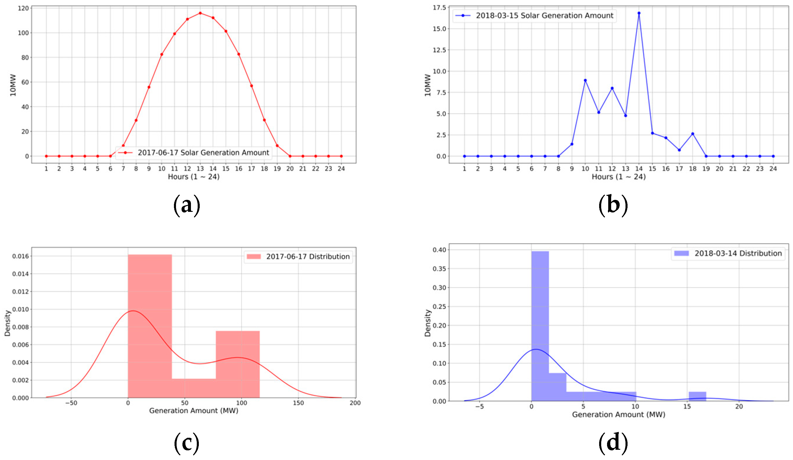
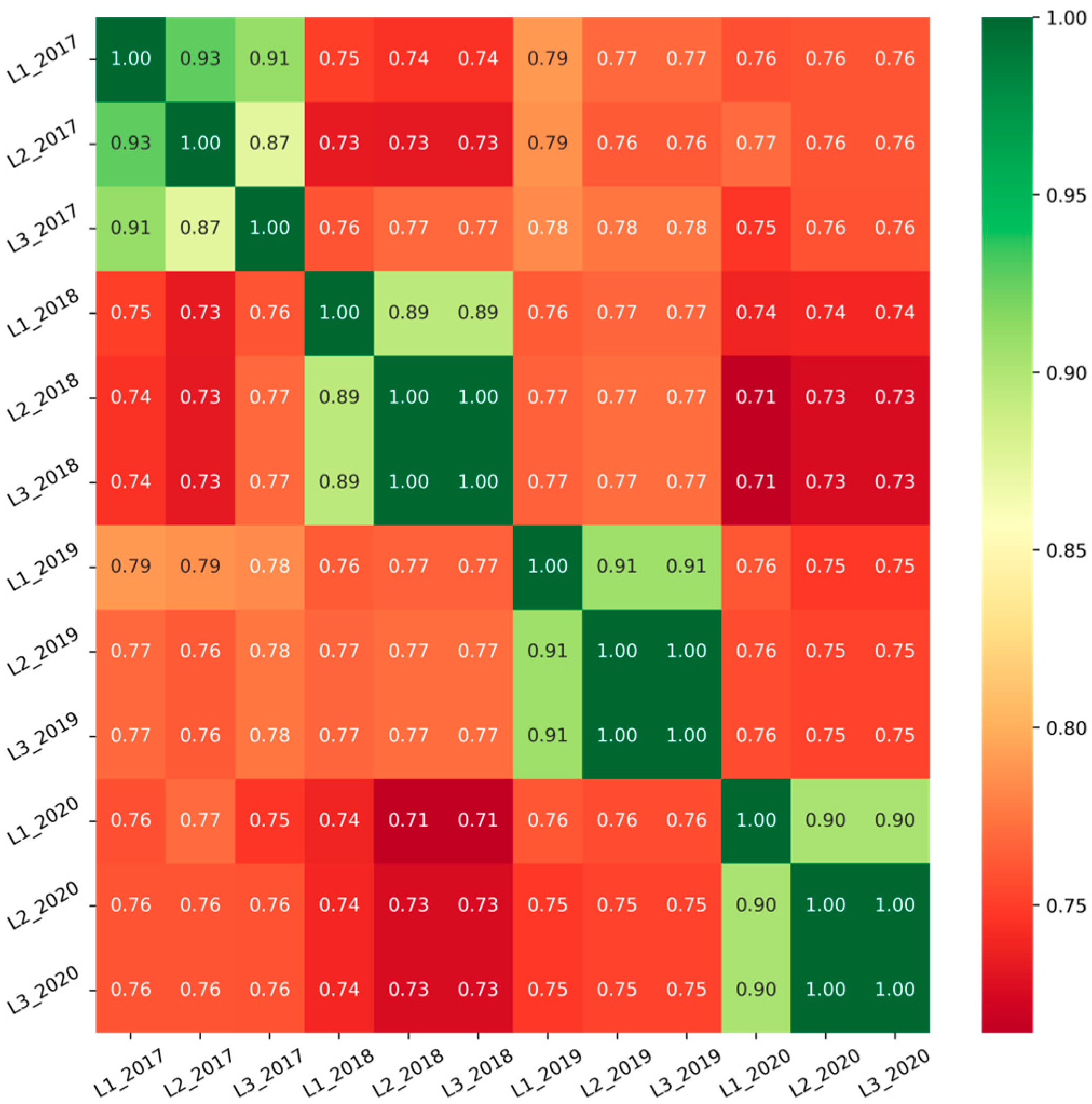
4.1. Dataset Analysis

The acquired dataset [6] was imported from the public portal provided by the Korean government, which shows the solar power generation amount in the solar power plants located in the three provinces (Sejong-si, Youngnam-gun, Ansan-si; $L_1,L_2,L_3$). The cumulation period was from 1 January 2017 to 31 August 2021 with hourly measurements. Such a time-domain dataset has two main repeated periodical data time-unit frames: day (24 h) and year. Monthly, weekly, and seasonally do not show a cyclic pattern, which was not considered. The generation amount repeatedly displays a similar trend in those two units, such that $n\left(D_i^{\left(\exists T\right)}\right)=24$ or $8760$, and $\delta \left(D_i^{\left(\exists T\right)},D_{i^{\prime }}^{\left(\exists T\right)} s.t. n\left(D_i^{\left(\exists T\right)}\right)=24\mathrm{or}8760\right)\ll \delta \left(D_i^{\left(\exists T\right)},D_{i^{\prime }}^{\left(\exists T\right)} s.t. n\left(D_i^{\left(\exists T\right)}\right)\ne 24\mathrm{or}8760\right)$.

The following figures show the ideal sample and the defective sample of daily energy collection. Figure 2a displays a smooth curve starting around 7:00 a.m., reaches its peak at 13:00 p.m., and halts the generation around 20:00 p.m. Let this ideal form be (12). In (12), $\max S\left({𝓉}_h\right)\to \frac{d}{d𝓉}{S}^{\prime }\left({𝓉}_h\right)=0$, and $12\le \mathrm{argmax} S\left({𝓉}_h\right)\le 14$. Therefore, $\frac{d}{d𝓉}{S}^{\prime }\left(\mathrm{argmax} S\left({𝓉}_h\right)\pm c\right)<\frac{d}{d𝓉}{S}^{\prime }\left({𝓉}_h\ne \mathrm{argmax} S\left({𝓉}_h\right)\pm c\right)$, $2\cdot \left(\frac{1+2c}{24}\right)\approx \frac{n\left({{\displaystyle \cup }}_{\forall {𝓉}_h}\left({𝓉}_h\to \left(S\left({𝓉}_h\right)\approx 0\right)\right)\right)}{24}$, where $c\in \mathbb{N}$ indicates the proximal hours surrounding $\mathrm{argmax} S\left({𝓉}_h\right)$, and this explains Figure 2c,d. In contrast, Figure 2a,b consists of unstable peaks without intuitive periodical variation, which has the form of (13) and the most distinctive large density at $S\left({𝓉}_h\right)\approx 0$.

$$S\left({𝓉}_h\right)=\{\begin{array}{c}if 6<h<20, S\left({𝓉}_h\right)\approx \frac{e^{-\frac{1}{2}\left(\frac{{𝓉}_h-\mu \left(\forall {𝓉}_h\right)}{\sigma \left(\forall {𝓉}_h\right)}\right)}}{\sigma \left({𝓉}_h\right)\sqrt{2\pi }}+ϵ\\ otherwise, S\left({𝓉}_h\right)\approx 0\end{array}$$

(12)

$$S\left({𝓉}_h\right)=\{\begin{array}{c}if 6<h<20, S\left({𝓉}_h\right)\le \frac{e^{-\frac{1}{2}\left(\frac{{𝓉}_h-\mu \left(\forall {𝓉}_h\right)}{\sigma \left(\forall {𝓉}_h\right)}\right)}}{\sigma \left({𝓉}_h\right)\sqrt{2\pi }}+ϵ\\ otherwise, S\left({𝓉}_h\right)\approx 0\end{array}$$

(13)

The non-IID property resembles risk while collaborating to aggregate the individual local models. It was noted that the predefined non-IID case C to quantify its internal non-IID degree, where $\frac{1}{{{\displaystyle \cup }}_{\forall j}1}{{\displaystyle \sum }}_{\forall j}\left(\delta \left(y_i,y_{i^{\prime }}\right)\right)\gg 0$. Case C is computed through ${{\displaystyle \cup }}_{years}\frac{1}{24}{\displaystyle \sum }_{i=1}^{t=24}\left(\left|{\widehat{L}}_i-{\widehat{L}}_{i^{\prime }}\right|\right)\equiv \left(7\right):=\widehat{\delta }\left(L_i,L_{i^{\prime }}\right)$, and ${\widehat{L}}_{\left(i,j\right)}={{\displaystyle \cup }}_{\forall j}{\widehat{L}}_{\left(i,j\right)}, s.t. {\widehat{L}}_{\left(i,j\right)}=\frac{L_{\left(i,j\right)}-\underset{\forall j}{\max }{L}_{\left(i,j\right)}}{\underset{\forall j}{\max }{L}_{\left(i,j\right)}-\underset{\forall j}{\min }{L}_{\left(i,j\right)}}$.

Table 1. $\widehat{\delta }\left(L_i,L_{i^{\prime }}\right)$ values.

	$$\widehat{\mathit{\delta }}\left({\mathit{L}}_1,{\mathit{L}}_2\right)$$	$$\widehat{\mathit{\delta }}\left({\mathit{L}}_1,{\mathit{L}}_3\right)$$	$$\widehat{\mathit{\delta }}\left({\mathit{L}}_2,{\mathit{L}}_3\right)$$
2017	1.60 ± 0.85	1.55 ± 1.03	1.86 ± 0.90
2018	1.66 ± 0.95	1.60 ± 0.99	1.86 ± 0.91
2019	1.57 ± 0.88	1.60 ± 0.99	1.83 ± 0.91
2020	1.71 ± 0.75	1.61 ± 1.00	1.97 ± 0.86
August 2021	1.87 ± 0.87	1.64 ± 0.97	1.98 ± 0.86
Overall	1.67 ± 0.87	1.60 ± 1.00	1.89 ± 0.89

displays the $\mu \left(\widehat{\delta }\left(L_i,L_{i^{\prime }}\right)\right)\pm \sigma \left(\widehat{\delta }\left(L_i,L_{i^{\prime }}\right)\right)$ in each year and the overall values combined for all the periods. Based on this, assuming that the dataset shares similar features in the synchronous time domain, it is certain that the degree of the non-IID attribute is: $\widehat{\delta }\left(L_2,L_3\right)>\widehat{\delta }\left(L_1,L_3\right)>\widehat{\delta }\left(L_1,L_2\right)$. Additionally, although $L_{\forall i}$ shares a synchronous direct source, the geographical distance between the entities should be pondered. The relationship of the Euclidean distance is $\left(L_2,L_3\right)\approx 330>\left(L_1,L_3\right)\approx 230>\left(L_1,L_2\right)\approx 130,$ where the unit is kilometers, which is identical to the degree of non-IID. This can be roughly interpreted as the proximal distance is likely to share analogous features, and utilizing those factors can be beneficial; this claim is validated in Section 4.3.

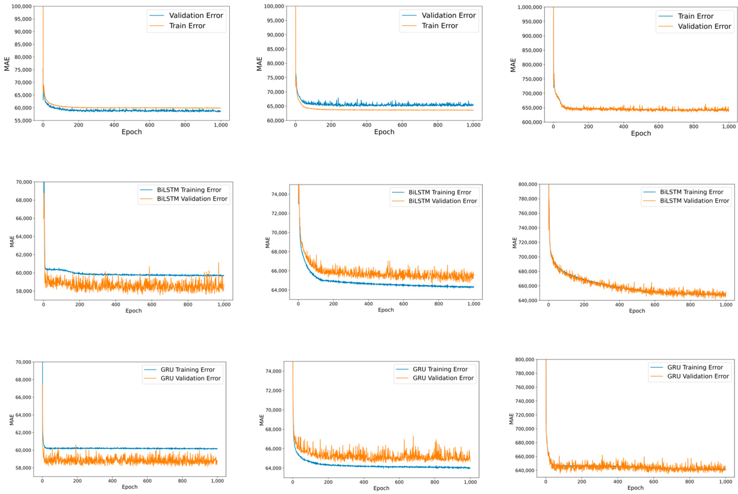
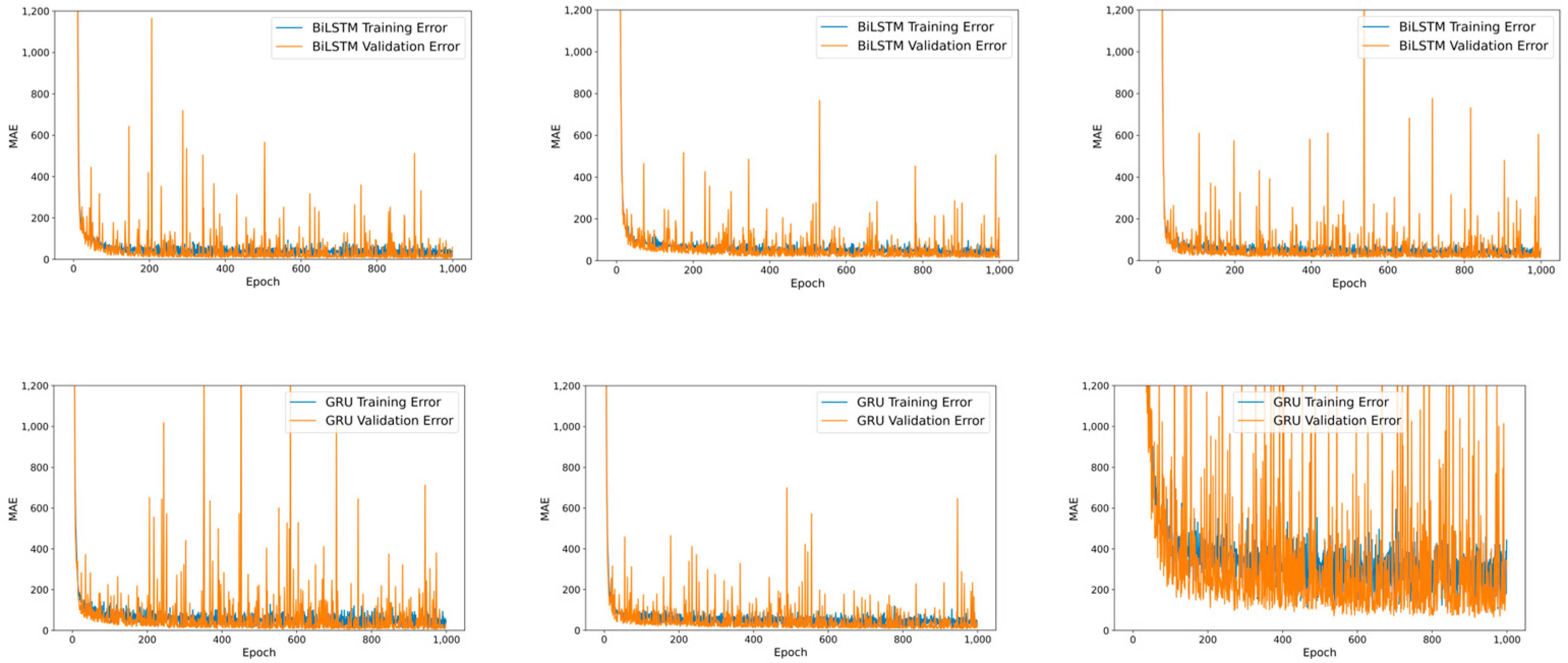
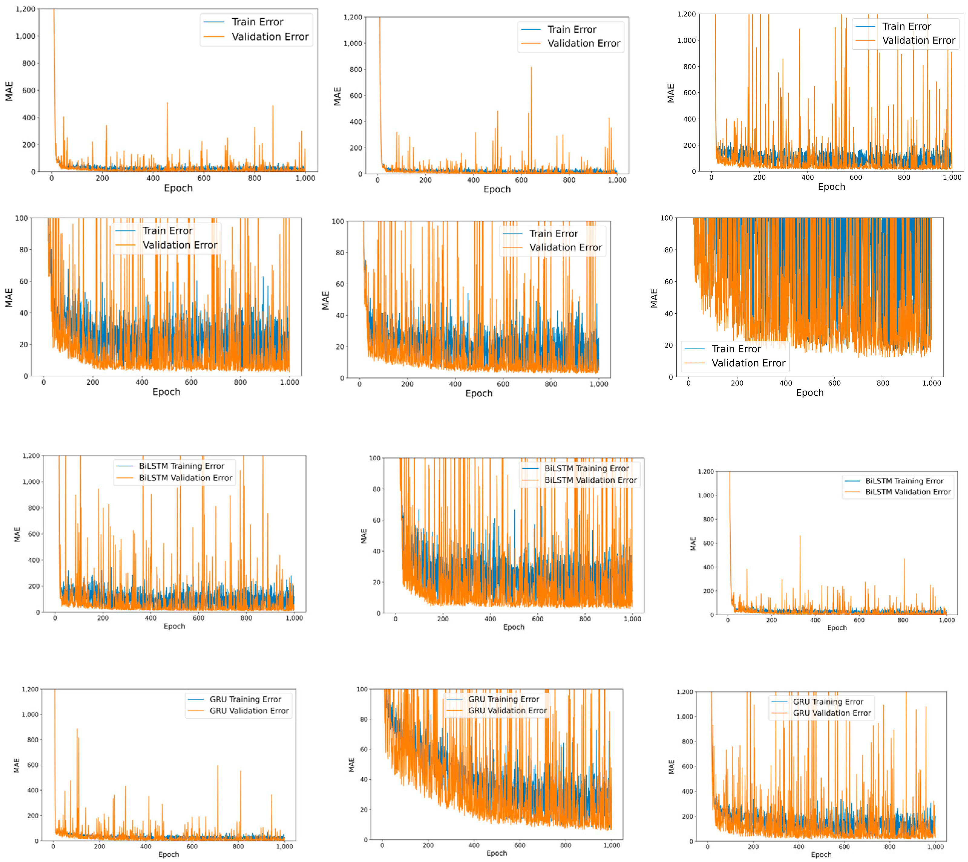
4.2. Training RNN-Based Models in Local Client

Based on the collected dataset ($D_i\in L_i$), the experiment initially implements the three RNN-based models: LSTM, GRU, and BiLSTM, to train the solar energy generation amount. The training dataset is nominated with the other two $D_i$ ($x_{f=D_i}$) in the initial experiment setting, and the training label is target $D_{i^{\prime }}$ (e.g., $i=1,2,i^{\prime }=3$). The second experimental setting inserts all the $D_{\forall i}\ni x_{f=D_i}$ in the training dataset to train the single model (e.g., $i=1,2,3,i^{\prime }=1 or 2 or 3$). The third experiment independently trains three RNN-based models ($M_i$) with their unique $D_i$. Every experiment had an identical model structure with 1000 epochs, RNN-based model (64)-Dense (64)-Dense (32)-Dense (1), 32 batch size, Adam optimizer, ReLU activation function, mean-absolute-error loss function, 20% validation split from the training dataset, training dataset were January 2017–December 2020, and test dataset were January 2021–August 2021. The results of experiments 1 and 2 are shown in Figure 3, and experiment 3 is shown in Figure 4.

Compared to other experiments, the MAE of experiment 1 reveals to be lower than expected, with an average value of 58,202.96 (Local 1), 62,592.67 (Local 2), and 635,606.56 (Local 3) in LSTM. Local 3 shows the worst performance, approximately ten times larger than the other two local models. However, the average data value for all locals is 250,251.28, which the unit itself is considered large. This implies that a training dataset that incorporates past data is the compelling feature that must be fused. Assuming from the general knowledge that a more quality dataset volume enhances the performance, experiment 2 spends more resources than experiment 1 with additional features (i.e., an identical unit of target labels with a different period). The training was successful, lowering the average of MAE to 9.66 (Local 1), 71.93 (Local 2), and 75.47 (Local 3), which is a far better achievement than experiment 1. However, experiment 3 surpasses this with 1.28 (Local 1), 12.20 (Local 2), and 27.50 (Local 3). This implies that FL performance is unlikely to be superior to the locally trained model when forecasting its individual target value. The following subsection explicates this in detail. The overall results are shown in

Table 2. Final training result for experiments 1–3.

Experiment 1
	Local 1		Local 2		Local 3
	Train	Val	Train	Val	Train	Val
LSTM	60,298.26	58,202.96	64,383.79	62,592.67	662,806.25	635,606.56
GRU	60,169.04	58,801.27	64,059.05	64,715.78	640,914.86	641,708.94
BiLSTM	59,735.69	58,777.66	64,374.08	65,708.52	646,646.01	651,371.92
Experiment 2
	Local 1		Local 2		Local 3
	Train	Val	Train	Val	Train	Val
LSTM	39.41	9.66	93.16	71.93	374.10	75.47
GRU	47.73	36.67	30.86	27.75	443.16	310.01
BiLSTM	41.74	58.56	35.78	12.73	56.57	59.75
Experiment 3
	Local 1		Local 2		Local 3
	Train	Val	Train	Val	Train	Val
LSTM	21.56	1.28	27.41	12.20	159.37	27.50
GRU	29.86	19.76	32.15	6.80	204.22	30.82
BiLSTM	22.43	1.81	14.13	8.16	119.58	16.97

.

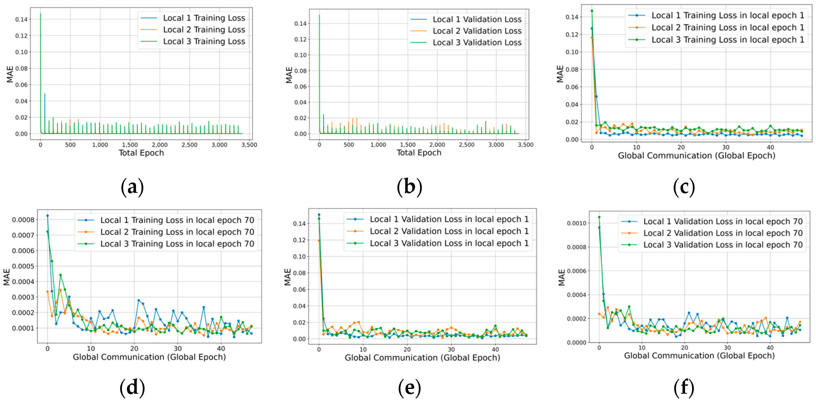
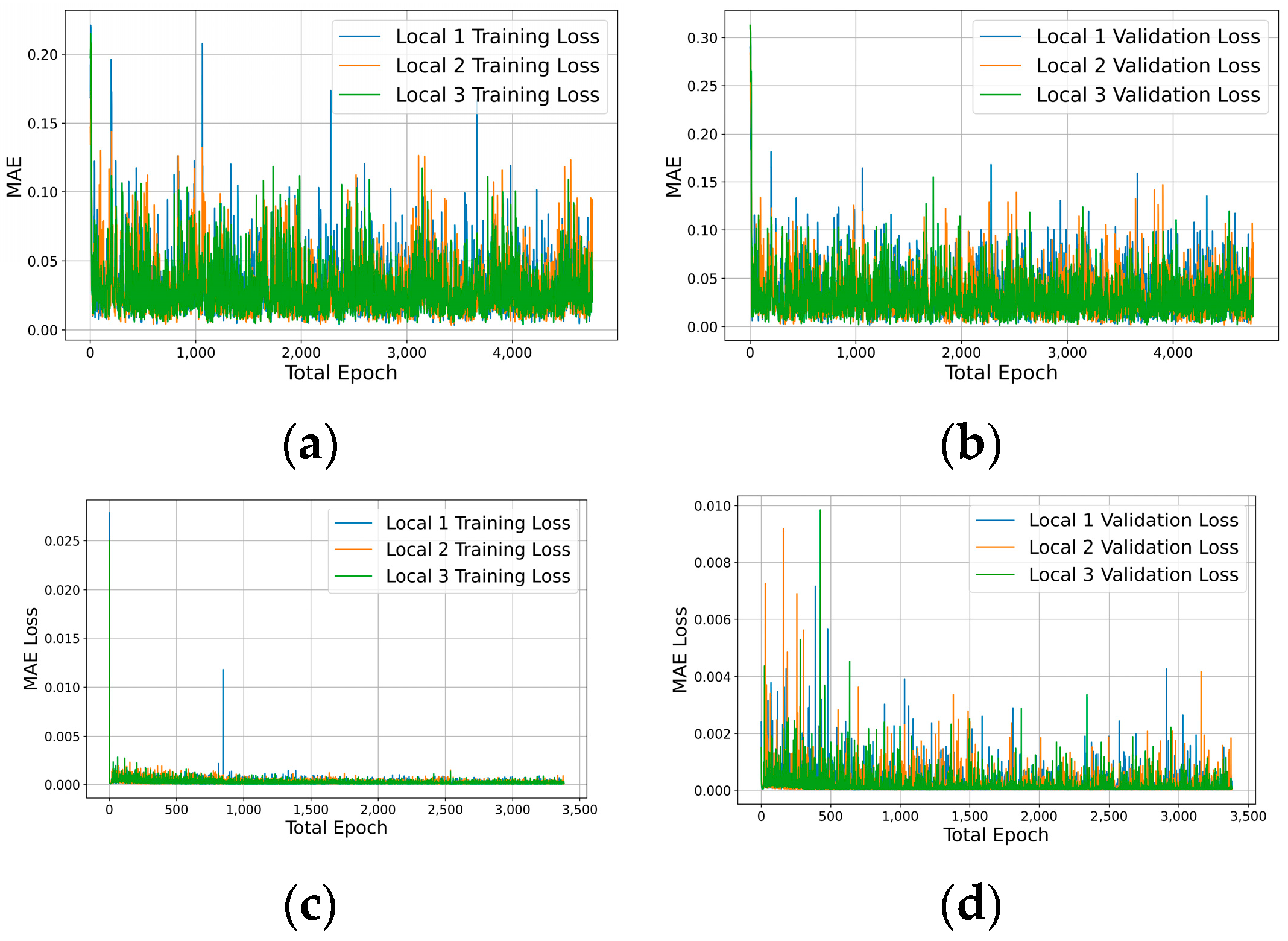
4.3. Merging Heterogeneous Local Models in FL

The MAE of the individual local models in Section 4.2 results shows that $MAE\left(L_1\right)<MAE\left(L_2\right)<MAE\left(L_3\right)$ in experiments 1–3. This relation corresponds to $\widehat{\delta }\left(L_2,L_3\right)>\widehat{\delta }\left(L_1,L_3\right)>\widehat{\delta }\left(L_1,L_2\right)\leftrightarrow$ non-IID degree: $L_3>L_2>L_1$. Furthermore, Figure 5 shows the heatmap that displays the Pearson correlation of the yearly period dataset. $PCC\left(L_{\left(i,year\right)},L_{\left(i^{\prime },yea{r}^{\prime }\right)}\right)>0$, $0.71\le PCC\left(L_{\left(i,year\right)},L_{\left(i^{\prime },yea{r}^{\prime }\right)}\right)\le 0.79$, and $0.87\le PCC\left(L_{\left(i,year\right)},L_{\left(i^{\prime },year\right)}\right)\le 1$, where $PCC\left(x,y\right)$ denotes the Pearson Correlation Coefficient of input $x,y,$ and $year\ne yea{r}^{\prime }$, $i\ne i^{\prime }$. This implies that the unmatched period encompasses a relatively low statistical feature than the equivalent year dataset, which is likely to be a non-IID dataset in terms of the period (i.e., dates rotate with the years).

Based on the locally trained models with a monthly dataset with 70 epochs, it merges them to create $\mathbb{G}$ and iteratively propagates the $\underset{\mathrm{T}\to 48}{\lim }{\mathbb{G}}^{\left(T\right)}\to L_{\forall i}^{\left(T\right)}$ (i.e., 12 months, 4 years), where the overall training epoch is $70\cdot 12\cdot 4=3360$. The result is shown in Figure 5, where the loss values are trained from ${\mathbb{G}}_{\left(train=L_{\exists i}\right)}^{\left(T-1,t=70\right)}\to f\left(D_{\exists i}^{\left(T\right)}\right)$, $\min \mathbb{L}\left(f\left(D_{\exists i}^{\left(T\right)},W_{\exists i}^{\left(T,t\right)}\right),y_{\exists i}\right)\to W_{\exists i}^{\left(t+1\right)}=\mathsf{\Delta }{W}_{\exists i}^{\left(t\right)}+W_{\exists i}^{\left(t\right)}$, and $\mathbb{L}\left(f\left(D_i\right),y_i\right)$; training and validation datasets are shown in Figure 6a,b. At every global epoch, a surge in loss is observed. Although $\underset{T\to \mathbb{T}=48}{\lim }(\underset{t\to \mathsf{𝕥}=20}{\lim }\mathbb{L}\left(f\left(D_{\exists i}^{\left(T\right)},W_{\exists i}^{\left(T,t\right)}\right),y_{\exists i}\right))\approx 0$, which satisfies the objective function, $\frac{1}{{{\displaystyle \sum }}_{\forall i}1}{\displaystyle \sum }_{\forall i}{W}_i^{\left(T\right)}={\mathbb{G}}^{\left(T\right)}\to \mathbb{L}\left(f\left(D_{\exists i}^{\left(T\right)},W_{\exists i}^{\left(T,t=\mathsf{𝕥}\right)}\right),y_{\exists i}\right)<\mathbb{L}\left(f\left(D_{\exists i}^{\left(T\right)},W_{\exists i}^{\left(T+1,t=1\right)}\right),y_{\exists i}\right)$. Figure 6c–f shows the loss of initial and final local epoch $\mathbb{L}(f\left(D_{\exists i}^{\left(T\right)},W_{\exists i}^{\left(\forall T,t=1\right)}\right), \mathbb{L}(f\left(D_{\exists i}^{\left(T\right)},W_{\exists i}^{\left(\forall T,t=70\right)}\right)$, and results show that $\mathbb{L}(f\left(D_{\exists i}^{\left(T\right)},W_{\exists i}^{(T>2,t)}\right)$ tend to converge. Note that the LSTM layer was used in local models.

This denotes that after the merge in global communication, further training must be accompanied for optimal convergence, and the following experiment proves this. After 1000 local epochs in the LSTM model, the experiment merged the locals, and the outcomes were unsatisfactory while predicting the three test datasets, generating the MAE average shown in

Table 3. Average MAE result for local combinations.

	Local 1	Local 2	Local 3
FedAvg ($L_1,L_2,L_3$)	472,308.44	516,164.47	1,334,568.25
FedAvg ($L_1,L_2$)	183,788.52	220,938.30	1,605,387.38
FedAvg ($L_1,L_3$)	11,498.82	30,333.07	1,790,837.25
FedAvg ($L_2,L_3$)	228,898.06	201,307.98	2,012,914.50

. Furthermore, experiments were conducted on the different combinations of locals while aggregation, such as combining only local models (1, 2), (2, 3), and (1, 3). The results are shown in Table 3, along with the performance mentioned above.

Lemma 1.

Loss in FL regression (i.e., $\mathbb{L}\left(\mathit{y},f\left(x\right)\right):=\frac{1}{n}{\displaystyle \sum }_{\forall i}{\left({\mathit{y}}_i-f\left({\mathit{x}}_i\right)\right)}^2$

) converges such that $\underset{T\to \mathbb{T}}{\lim }(\underset{t\to \mathsf{𝕥}}{\lim }\mathbb{L}\left(f\left({\mathit{D}}_i^{\left(T\right)},{\mathit{W}}_i^{\left(T,t\right)}\right),{\mathit{y}}_{\exists i}\right))\approx 0$ in the ${ℝ}^d$ loss space where $\left(\mathbb{T},\mathsf{𝕥},d\right)\in \mathbb{N}$

, while $\frac{1}{{{\displaystyle \sum }}_{\forall i}1}{\displaystyle \sum }_{\forall i}{\mathit{W}}_i^{\left(T\right)}={\mathbb{G}}^{\left(T\right)}\to \mathbb{L}\left(f\left({\mathit{D}}_{\exists i},{\mathit{W}}_{\exists i}^{\left(T,t=\mathsf{𝕥}\right)}\right),{\mathit{y}}_{\exists i}\right)<\mathbb{L}\left(f\left({\mathit{D}}_{\exists i},{\mathit{W}}_{\exists i}^{\left(T+1,t=1\right)}\right),{\mathit{y}}_{\exists i}\right)$

Theorem 1.

Based on Lemma, additional local training is required s.t. $\left(\mathbb{T},\mathsf{𝕥}\right)\ge 2,$ after $\frac{1}{{{\displaystyle \sum }}_{\forall i}1}{\displaystyle \sum }_{\forall i}{\mathit{W}}_i^{\left(T\right)}={\mathbb{G}}^{\left(T\right)}\to \underset{T\to \mathbb{T}}{\lim }(\underset{t\to \mathsf{𝕥}}{\lim }(\underset{\forall i}{\min }\mathbb{L}\left(f\left({\mathit{D}}_{\exists i}^{\left(T\right)},{\mathit{W}}_{\exists i}^{\left(T,t\right)}\right),{\mathit{y}}_{\exists i}\right)))$ in FL regression.

Proof of Theorem 1.

Empirical experiments—Experiments results in Table 2 and Figure 5 show that the theorem is true. Note that if $\left(\mathbb{T},\mathsf{𝕥}\right)=1\to \mathsf{\Delta }{W}_i^{\left(t\right)}=\varnothing$, and $\left(\mathbb{T},\mathsf{𝕥}\right)>1\to \mathsf{\Delta }{W}_i^{\left(t\right)}\ne \varnothing$, and $\mathsf{\Delta }{W}_i^{\left(t\right)}>0$, it satisfies (3). □

4.4. Federated Learning on Periodical Update

This section focuses on exploring the impact of global periodical collaboration, which is considered a vital factor while achieving convergence in FL. While total epochs are identical, the experiment considers three following periodical aggregation cases:

• Case $\mathcal{A}$. Daily update period, such that $\mathsf{𝕥}=24$, and $\mathbb{T}=\frac{c}{\mathsf{𝕥}}$ in (3).
• Case $ℬ$. Monthly period, such that $\mathsf{𝕥}=24\cdot Days$, and $\mathbb{T}=\frac{c}{\mathsf{𝕥}\cdot Days}$ in (3).
• Case $\mathcal{C}$. Yearly period, such that $\mathsf{𝕥}=24\cdot Days\cdot Months$, and $\mathbb{T}=\frac{c}{\mathsf{𝕥}\cdot Days\cdot Months}$ in (3).

All the cases have identical total epochs ($=\mathsf{𝕥}\cdot \mathbb{T}=3384$) and equivalent layer structures using LSTM and hyperparameters to former experiments in this Section 4. Case $\mathcal{A}$ results are shown in Figure 7a,b, with unstable convergence and relatively high loss values. Case $ℬ$ was already conducted and delivered in Figure 6a,b, and case $\mathcal{C}$ results are displayed in Figure 7c,d. In general, case $\mathcal{C}$ had the best performance, with a much smaller loss (i.e., when observing the scale of the suggested Figure 7a–d and stable trajectory compared to other cases). This implies that more local database volume will incorporate better convergence when training FL.

5. Conclusions

FL is a collaborative framework in a distributed system that accommodates a synergy effect among locally trained models with independently collected datasets from its unique environment. Aggregating the independently trained heterogeneous models construct a powerful global model by absorbing various features that enhance generalization and reduce bias. FL regression is widely impacted by the spatiotemporal features, where FL operates in a decentralized system that subsumes the geographical distance between the local units, and such curated datasets tend to be non-IID, which must take account of the timely global update with period while training the FL. The learning trajectory of FL is most likely to diverge when the adjustments are asynchronous or the assemblage does not mitigate the heterogeneous properties. This implies that combining diverse and unique local models trained with non-IID datasets in FL must be effectively aggregated in a way that directs the global model to return a high prediction rate.

This paper explores regression models in the FL, defining the frequent non-IID cases in real-life regression problems and discovering the temporal non-IID combination method via theoretical analysis and empirical experiments. This work utilized the solar energy generation dataset acquired from the three regions in South Korea and trained three types of RNN-based models, and showed that the improvement of conglomerating local regression models in the FL network correlates to the non-IID degree of the local dataset. This paper quantitively assessed the local non-IID degree by examining the dataset and observing the FL performance, which validated that the non-IID attribute hinders convergence during iterative aggregation in regression. This paper also suggested and proved that the global update period is a decisive factor that determines the performance of the FL through multiple experiments with a 4.5-year-long dataset, which is a novel approach and pragmatic matter that must be optimized when applied to a real-practice Smart Grid environment.

This study offers a collaboration scheme to build an efficient FL-based regression model that can be utilized in the decentralized power grid system, which encompasses the geographical features that are primarily nonadjacent and independently operate to each neighbor’s power source. Through theoretical analysis and experiments suggested in this study, the author hopes this FL research provides the practical approach and perspective to a successful operation in a diversified disseminated energy grid system such as Smart Grid and Micro Grid via FL.

References

1. McMahan, B.; Moore, E.; Ramage, D.; Hampson, S.; Arcas, B.A. Communication-efficient learning of deep networks from decentralized data. In Artificial Intelligence and Statistics; PMLR: Cambridge, MA, USA, 2017; pp. 1273–1282. [Google Scholar]
2. Li, X.; Huang, K.; Yang, W.; Wang, S.; Zhang, Z. On the convergence of fedavg on non-iid data. arXiv 2019, arXiv:1907.02189. [Google Scholar]
3. Gadekallu, T.R. Federated Learning for Big Data: A Survey on Opportunities, Applications, and Future Directions. arXiv 2021, arXiv:2110.04160. [Google Scholar]
4. Zhan, Y.; Zhang, J.; Hong, Z.; Wu, L.; Li, P.; Guo, S. A Survey of Incentive Mechanism Design for Federated Learning. IEEE Trans. Emerg. Top. Comput. 2021, 10, 1035–1044. [Google Scholar] [CrossRef]
5. Karimireddy, S.P.; Kale, S.; Mohri, M.; Reddi, S.; Stich, S.; Suresh, A.T. Scaffold: Stochastic controlled averaging for federated learning. In International Conference on Machine Learning; PMLR: Cambridge, MA, USA, 2020; pp. 5132–5143. [Google Scholar]
6. Korea Public Data Portal. Available online: https://www.data.go.kr/data/15003553/fileData.do (accessed on 21 December 2022).
7. You, S. A Cyber-secure Framework for Power Grids Based on Federated Learning. Eng. Arch. 2020. [Google Scholar] [CrossRef]
8. Massaoudi, M.; Abu-Rub, H.; Refaat, S.S.; Chihi, I.; Oueslati, F.S. Deep Learning in Smart Grid Technology: A Review of Recent Advancements and Future Prospects. IEEE Access 2021, 9, 54558–54578. [Google Scholar] [CrossRef]
9. Taik, A.; Nour, B.; Cherkaoui, S. Empowering Prosumer Communities in Smart Grid with Wireless Communications and Federated Edge Learning. IEEE Wirel. Commun. 2021, 28, 26–33. [Google Scholar] [CrossRef]
10. Zhai, S.; Jin, X.; Wei, L.; Luo, H.; Cao, M. Dynamic Federated Learning for Gmec With Time-Varying Wireless Link. IEEE Access 2021, 9, 10400–10412. [Google Scholar] [CrossRef]
11. Liu, H.; Zhang, X.; Shen, X.; Sun, H. A federated learning framework for smart grids: Securing power traces in collaborative learning. arXiv 2021, arXiv:2103.11870. [Google Scholar]
12. Wen, M.; Xie, R.; Lu, K.; Wang, L.; Zhang, K. FedDetect: A Novel Privacy-Preserving Federated Learning Framework for Energy Theft Detection in Smart Grid. IEEE Internet Things J. 2021, 9, 6069–6080. [Google Scholar] [CrossRef]
13. Zhao, L.; Li, J.; Li, Q.; Li, F. A Federated Learning Framework for Detecting False Data Injection Attacks in Solar Farms. IEEE Trans. Power Electron. 2021, 37, 2496–2501. [Google Scholar] [CrossRef]
14. Li, D.; Luo, Z.; Cao, B. Blockchain-based federated learning methodologies in smart environments. Clust. Comput. 2021, 25, 2585–2599. [Google Scholar] [CrossRef]
15. Al-Quraan, M.; Khan, A.; Centeno, A.; Zoha, A.; Imran, M.A.; Mohjazi, L. FedTrees: A Novel Computation-Communication Efficient Federated Learning Framework Investigated in Smart Grids. arXiv 2022, arXiv:2210.00060. [Google Scholar]
16. Wang, Y.; Bennani, I.L.; Liu, X.; Sun, M.; Zhou, Y. Electricity consumer characteristics identification: A federated learning approach. IEEE Trans. Smart Grid 2021, 12, 3637–3647. [Google Scholar] [CrossRef]
17. Zhao, Y.; Xiao, W.; Shuai, L.; Luo, J.; Yao, S.; Zhang, M. A Differential Privacy-enhanced Federated Learning Method for Short-Term Household Load Forecasting in Smart Grid. In Proceedings of the 2021 7th International Conference on Computer and Communications (ICCC), Chengdu, China, 10–13 December 2021; pp. 1399–1404. [Google Scholar] [CrossRef]
18. Fernandez, J.D.; Menci, S.P.; Lee, C.; Fridgen, G. Secure Federated Learning for Residential Short Term Load Forecasting. arXiv 2021, arXiv:2111.09248. [Google Scholar]
19. Zhou, X.; Feng, J.; Wang, J.; Pan, J. Privacy-preserving household load forecasting based on non-intrusive load monitoring: A federated deep learning approach. PeerJ Comput. Sci. 2022, 8, e1049. [Google Scholar] [CrossRef] [PubMed]
20. Savi, M.; Fabrizio, O. Short-term energy consumption forecasting at the edge: A federated learning approach. IEEE Access 2021, 9, 95949–95969. [Google Scholar] [CrossRef]
21. Taik, A.; Cherkaoui, S. Electrical Load Forecasting Using Edge Computing and Federated Learning. In Proceedings of the ICC 2020–2020 IEEE International Conference on Communications (ICC), Dublin, Ireland, 7–11 June 2020; pp. 1–6. [Google Scholar] [CrossRef]
22. Zhang, P.; Wang, C.; Jiang, C.; Han, Z. Deep Reinforcement Learning Assisted Federated Learning Algorithm for Data Management of IIoT. IEEE Trans. Ind. Inform. 2021, 17, 8475–8484. [Google Scholar] [CrossRef]
23. Saputra, Y.M.; Hoang, D.T.; Nguyen, D.N.; Dutkiewicz, E.; Mueck, M.D.; Srikanteswara, S. Energy Demand Prediction with Federated Learning for Electric Vehicle Networks. In Proceedings of the 2019 IEEE Global Communications Conference (GLOBECOM), Waikoloa, HI, USA, 9–13 December 2019; pp. 1–6. [Google Scholar]
24. Huang, X.; Li, P.; Yu, R.; Wu, Y.; Xie, K.; Xie, S. Fedparking: A federated learning based parking space estimation with parked vehicle assisted edge com-puting. IEEE Trans. Veh. Technol. 2021, 70, 9355–9368. [Google Scholar] [CrossRef]
25. Zhang, Y.; Tang, G.; Huang, Q.; Wang, Y.; Wu, K.; Yu, K.; Shao, X. FedNILM: Applying Federated Learning to nilm Applications at the Edge. In IEEE Transactions on Green Communications and Networking; IEEE: Piscataway Township, NJ, USA, 2022; p. 1. [Google Scholar] [CrossRef]
26. Hudson, N.; Hossain, J.; Hosseinzadeh, M.; Khamfroush, H.; Rahnamay-Naeini, M.; Ghani, N. A Framework for Edge Intelligent Smart Distribution Grids via Federated Learning. In Proceedings of the 2021 International Conference on Computer Communications and Networks (ICCCN), Athens, Greece, 19–22 July 2021; pp. 1–9. [Google Scholar] [CrossRef]
27. Nightingale, J.S.; Wang, Y.; Zobiri, F.; Mustafa, M.A. Effect of Clustering in Federated Learning on Non-IID Electricity Consumption Prediction. In Proceedings of the 2022 IEEE PES Innovative Smart Grid Technologies Conference Europe (ISGT-Europe), Novi Sad, Serbia, 10–12 October 2022; pp. 1–5. [Google Scholar] [CrossRef]
28. Briggs, C.; Fan, Z.; Andras, P. Federated learning for short-term residential energy demand forecasting. arXiv 2021, arXiv:2105.13325. [Google Scholar]
29. Yan, G.; Hao, W.; Jian, L. Seizing Critical Learning Periods in Federated Learning. In Proceedings of the AAAI Conference on Artificial Intelligence; AAAI Press: Palo Alto, CA, USA, 2022. [Google Scholar]
30. Lu, Y.; Huang, X.; Zhang, K.; Maharjan, S.; Zhang, Y. Blockchain Empowered Asynchronous Federated Learning for Secure Data Sharing in Internet of Vehicles. IEEE Trans. Veh. Technol. 2020, 69, 4298–4311. [Google Scholar] [CrossRef]
31. Lim, W.Y.B.; Xiong, Z.; Miao, C.; Niyato, D.; Yang, Q.; Leung, C.; Poor, H.V. Hierarchical Incentive Mechanism Design for Federated Machine Learning in Mobile Networks. IEEE Internet Things J. 2020, 7, 9575–9588. [Google Scholar] [CrossRef]
32. Lee, H.; Liu, Y.; Kim, D.; Li, Y. Robust Convergence in Federated Learning through Label-wise Clustering. arXiv 2021, arXiv:2112.14244. [Google Scholar]
33. Zhou, T.; Konukoglu, E. FedFA: Federated Feature Augmentation. arXiv 2023, arXiv:2301.12995. [Google Scholar]
Figure 1. Federated Learning architecture visualization in solar energy generation environment.
Electronics 12 01580 g001
Figure 2. Visualization sample (a,b) of daily solar energy generation and its distribution (c,d).
Electronics 12 01580 g002
Figure 3. RNN-based models’ training MAE result for experiments 1 and 2: rows 1–3 and column 1 display the MAE-LSTM, BiLSTM, and GRU with training dataset  ( D 1 , D 2 )  and target dataset  D 3 . Figures in rows 1–3 and columns 2–3 show MAE-LSTM, BiLSTM, and GRU with training dataset  ( D 1 , D 3 ) ( D 2 , D 3 ) , and target dataset  D 2 . D 1 , respectively. Figures in rows 4–6 columns 1–3 was trained with  ( D 1 , D 2 , D 3 ) , and their target set was  D 1 ,   D 2 , D 3 , respectively.
Electronics 12 01580 g003aElectronics 12 01580 g003b
Figure 4. LSTM training performance of experiment 3. Figures in row 1 display LSTM results with a scale of 0–1200, and row 2 has a narrow scale of 0–100. Figures in row 3 show the BiLSTM result, and row 4 shows the GRU result. The Figures in sequential columns in each row indicate local 1,2, and 3.
Electronics 12 01580 g004
Figure 5. Heatmap of the  P C C ( L ( i , y e a r ) , L ( i , y e a r ) ) .
Electronics 12 01580 g005
Figure 6. FL training results in training (a): validation loss (b), training loss at local epochs 1 and 70 (c,d), and validation loss at local epochs 1 and 70 (e,f).
Electronics 12 01580 g006
Figure 7. MAE values for FL: (a,b) the training and validation losses on daily updates; (c,d) the training and validation loss for yearly updates.
Electronics 12 01580 g007