Article

Friction Feedforward Compensation Composite Control of Continuous Rotary Motor with Sliding Mode Variable Structure Based on an Improved Power Reaching Law

1
Beijing Key Laboratory of Performance Guarantee on Urban Rail Transit Vehicle, Beijing University of Civil Engineering and Architecture, Beijing 102616, China
2
Beijing Engineering Research Center of Monitoring for Construction Safety, Beijing University of Civil Engineering and Architecture, Beijing 102616, China
3
School of Mechanical and Power Engineering, Harbin University of Science and Technology, Harbin 150080, China
*
Author to whom correspondence should be addressed.
Electronics 2023, 12(6), 1447; https://doi.org/10.3390/electronics12061447
Submission received: 23 January 2023 / Revised: 10 March 2023 / Accepted: 14 March 2023 / Published: 18 March 2023
(This article belongs to the Special Issue Mechatronic Control Engineering Volume II)

Abstract

:
In order to meet the accuracy requirements and tracking performance of continuous rotary electro-hydraulic servo motor system under nonlinear uncertainty and strong disturbance factors, the sliding mode variable structure composite control strategy based on an improved power reaching law is proposed. Based on the principle of valve-controlled hydraulic motor, the state space model of the motor system is established, and a continuous friction model is adopted. Then, the genetic algorithm is used for parameter identification to determine the friction feedforward compensation scheme. In addition, an improved power reaching law is designed, which can adaptively adjust the system chattering according to the system state. The simulation results show that the sliding mode variable structure composite controller with the friction feedforward compensation can achieve a system frequency of 15 Hz, and tracking accuracy and response speed meet the double-decade index requirements, which improve the performance of continuous rotary electro-hydraulic servo motor.

1. Introduction

As an important device in flight simulation experiments, continuous rotary electro-hydraulic servo motor can reproduce the attitude angle change of the vehicle with the advantages of high frequency response, high accuracy and ultra-low speed [1,2,3]. However, the electro-hydraulic servo motor system is affected by frictional disturbances and other uncertain non-linear factors [4,5], which cause steady-state errors in the low-speed tracking state and cause crawling in severe cases.
Eliminating friction on mechanical devices is often extremely costly [6,7,8] and even impractical, and the best approach is to perform friction compensation from the control strategy. There have been numerous studies on friction compensation [9,10,11,12], and friction models that capture different friction phenomena have been established and introduced into electro-hydraulic servo control to greatly improve control accuracy. Meanwhile, sliding mode variable structure control (SMC) can change the structure of the controller according to the deviation of the system state from the sliding mode surface to drive it back to the pre-defined trajectory, so its control effect is independent of parameters and does not need to be identified online, which has strong robustness and other advantages. It is very suitable for engineering applications [13,14,15].
However, most classical friction models are derived from the static mapping relationship between relative velocity and friction with a symbolic function assigning the direction of the friction force, and this discontinuous or segmented continuous friction model can cause system instability [16,17,18]. For the slide-mode variable structure controller, the system state is continuously reciprocating along the slide-mode surface due to the switching function, resulting in the “chattering” phenomenon [19,20].
Some innovative studies have been conducted by scholars in recent years. M. Ahmadi et al. compensated the pitch and yaw angles of a multivariable (MIMO) dual-rotor system using a second-order sliding mode controller, and simulations were performed for both first- and second-order sliding mode controllers in all cases, and their advantages and disadvantages were investigated [21]. H. Hou et al. proposed a new full-order terminal sliding mode surface, and a new continuous terminal sliding mode control algorithm, which not only ensures robustness, but also continuity, makes the control algorithm more suitable for servomechanical systems [22]. Geqiang Li et al. use an analytical method to model the impact energy of the forging hammer and use a wavelet neural network PID control proposed algorithm to achieve closed-loop control of the pressure and speed of the direct-drive electro-hydraulic servo die forging hammer [23]. Tomonori Kato et al. propose a new control method for hybrid electric-pneumatic vertical-positioning devices (HVPDs) that reduce the motor load during material processing and use a perturbation observer to continuously estimate the external forces acting on the carrier table while maintaining high positioning performance [24].
According to the above problems of the controller and the impact of friction interference on the control accuracy of continuous rotary electro-hydraulic servo motor system, this paper designs a composite control strategy based on the improved power reaching law of the sliding mode variable structure combined with friction compensation, which can adaptively adjust the sliding mode chattering according to the system state until the equilibrium point is reached through Simulink simulation to prove the effectiveness of the designed control.

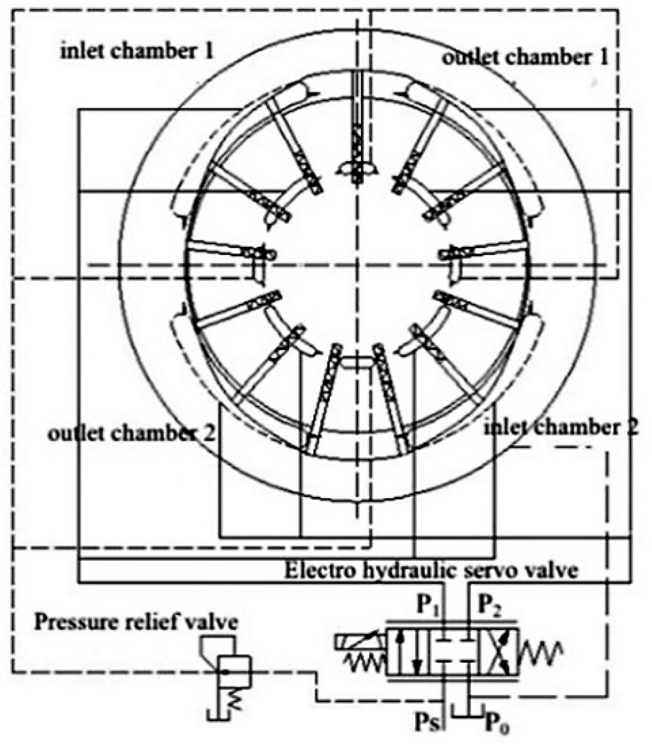
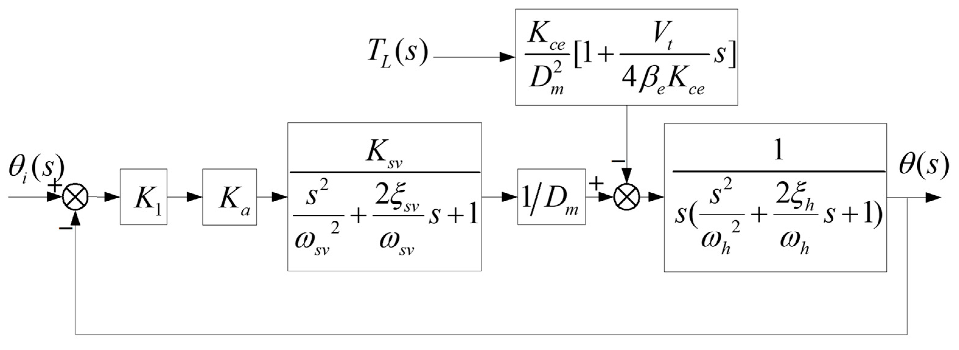
2. Continuous Rotary Motor State Space Modeling

Establishing a linearized flow equation for the orifice of the continuous rotary electro-hydraulic servo motor system shown in Figure 1, the orifice flow equation of the servo valve is Q L = K q x v K c p L , the Laplace transform is as follows:
Q L ( s ) = K q X v ( s ) K c P L ( s )
where, Q L is the load flow (m3/s); K q is the flow gain (m2/s); X v is the spool displacement (m); K c is the flow pressure coefficient (m3/(s·Pa)); and P L is the external load pressure (MPa).
The load flow rate of the motor during operation consists the flow rate required for a normal continuous rotation of the motor, the flow rate lost through internal and external leakage due to friction and external disturbance, and the additional flow rate due to oil compression, Q L = D m θ ˙ + C t m p L + V t 4 β e p ˙ L . Through the Laplace transform the load flow rate of the motor can be obtained.
Q L ( S ) = D m θ ( s ) s + C t m P L ( s ) + V t 4 β e P L ( s ) s
where, D m is the radian displacement (m3/rad); θ is the displacement (rad); C t m is the total leakage coefficient (m3/(s·Pa)); V t is the total volume of the connecting pipe, motor and servo valve chamber (m3); and β e is the effective volume modulus of elasticity (Pa).
Neglecting the effect of non-linear load factors such as static friction, the equations for the sum of the motor moments and the moment balance of the load are established based on Newton’s second law D m p L = J t θ ¨ + B m θ ˙ + G θ + T L . The Laplace transform is as follows:
D m P L ( s ) = J t θ ( s ) s 2 + B m θ ( s ) s + G θ ( s ) + T L ( s )
where, J t is the total rotational inertia of the motor and load after folding (kg·m2); B m is the viscous damping factor (N·m/(rad/s)); G is the spring stiffness of the load (N·m/rad); and T L is the load moment acting on the motor (N·m).
Assuming that the motor shaft is rigidly connected to the external load, no sliding friction is generated and G = 0. By combining Equations (1)–(3) and removing the intermediate variable QL, PL, the output angular displacement of continuous rotary motor θ ( s ) is related to the spool displacement of the electro-hydraulic servo valve X v ( s ) , and the sine disturbance torque T L ( s ) is as follows:
θ ( s ) = K q D m X v ( s ) K c e D m 2 ( 1 + V t 4 β e K c e s ) T L ( s ) s ( s 2 ω n 2 + 2 ξ h ω h s + 1 )  
where, ω h is the undamped hydraulic inherent frequency, rad/s, ω h = 4 β e D m 2 J t V t , ξ h is the hydraulic damping ratio (dimensionless), ξh = K c e D m J t β e V t + B m 4 D m , K c e is the total flow-pressure coefficient of the valve-controlled motor(m3/(s·Pa)), K c e = K c + C t m .
In a valve-controlled hydraulic motor system, the inherent frequency of the electro-hydraulic servo valve is higher than that of the hydraulic system and it is approximated as a second-order oscillation link, considering the influence of its dynamic performance on the hydraulic control system.
G s v ( s ) = Q 0 ( s ) I ( s ) = K s v s 2 ω s v 2 + 2 ξ s w ω s v s + 1
where, G S V is the electro-hydraulic servo valve transfer function; Q 0 is the no-load flow (m3/s), Q 0 = K q · X v ; K s v is the flow gain (m3/(s·A)); ω s v is the intrinsic frequency of the servo valve (rad/s); and ξ s v is the damping ratio of the servo valve.
Since the inherent frequency of the servo amplifier pair is much larger than the frequency band range of the hydraulic system, the transfer function is approximated as a proportional link.
I ( s ) U ( s ) = K a
where, K a is the gain of the amplifier (A/V).
According to the principle of hydraulic servo valve-controlled motor and Equations (1)–(6), a block diagram of the transfer function of continuous rotary motor system is established, as shown in Figure 2.
In the diagram, θ i ( s ) is the input angle command signal; θ ( s ) is the output motor angle of the system; K 1 is the main controller; T L ( s ) is the applied load torque, and the equation of the transfer function of the angular displacement of the motor output at no load is: θ ( s ) Q 0 ( s ) = 1 / D m s ( s 2 ω 2 h + 2 ξ h ω h s + 1 ) .
The state space model has a good mathematical mapping capability and allows direct observation of the changes in the state variables of the motor system. Ignoring the influence of the electro-hydraulic servo valve on the motor, it is simplified to a proportional link K. According to the parameters of each element of the continuous rotary motor, its state space model is established as:
{ x ˙ = A x + B u y = C x + D u
where, x ˙ = ( x 1 , x 2 , x 3 ) is the motor system state, x 1 = θ is the motor output angle, x 2 = θ ˙ is the motor angular velocity, x 3 = θ ¨ is the motor angular acceleration; A = [ 0 1 0 0 0 1 0 ω h 2 2 ξ h ω h ] ; B = [ 0 0 K 1 K a ω h 2 D m ] ; C = [ 1 0 0 ] ; D = 0 .

3. Continuous Rotary Motor Friction Torque Modeling and Compensation

3.1. Continuous Friction Model

Most classical friction models are derived from a static mapping relationship between relative velocity and friction, assigning the direction of friction with a symbolic function. Such discontinuous or segmented continuous friction models cause instability in the system, and when switching from static to dynamic friction, the friction triggers self-excited vibrations, leading to noise that reduces the resolution of the system and causes the motor to crawl. Therefore, a new continuous friction model proposed by Prof. C. Makkar is introduced here [16].
The model is suitable for the high precision control requirements of motors in a bi-directional rotation state, and can solve the problems of poor control accuracy and instability caused by the discontinuity of the friction model. To a certain extent, it can describe a variety of friction characteristics, covering the relevant properties of the Stribeck friction model, Maxwell friction model, Coulomb friction model, etc. The expression for the continuous friction model is:
T f ( q ˙ ) = k 1 ( tanh ( k 2 q ˙ ) tanh ( k 3 q ˙ ) ) + k 4 tanh ( k 5 q ˙ ) + k 6 q ˙
where, Tf is the value of the motor friction torque (N·m); k i R i = 1 ,   2 ,   ,   6 ; tanh is the hyperbolic tangent function; and q ˙ is the motor angular velocity (degree/sec).
At the same time, the continuous friction model has the following properties.
(1)
The model is symmetrical about the origin and applies to the motor’s bi-directional rotational state;
(2)
The static friction factor can be described when k6 = 0, where tanh ( k 2 q ˙ ) tanh ( k 3 q ˙ ) captures the Stribeck phenomenon, where the friction factor decreases as the speed of the motor system continues to increase;
(3)
k 6 q ˙ is viscous friction, capturing the viscosity resistance between the relative moving parts of the motor due to the viscosity of the lubricant;
(4)
k 4 tanh ( k 5 q ˙ ) indicates Coulomb friction and exists in a motor system without viscous friction.
The dynamic continuous friction model of the continuous rotary motor is determined according to the above equation, and further model parameter identification is carried out through experimental data acquisition to obtain accurate model parameter values in order to ensure a better control effect after compensation based on the friction model.

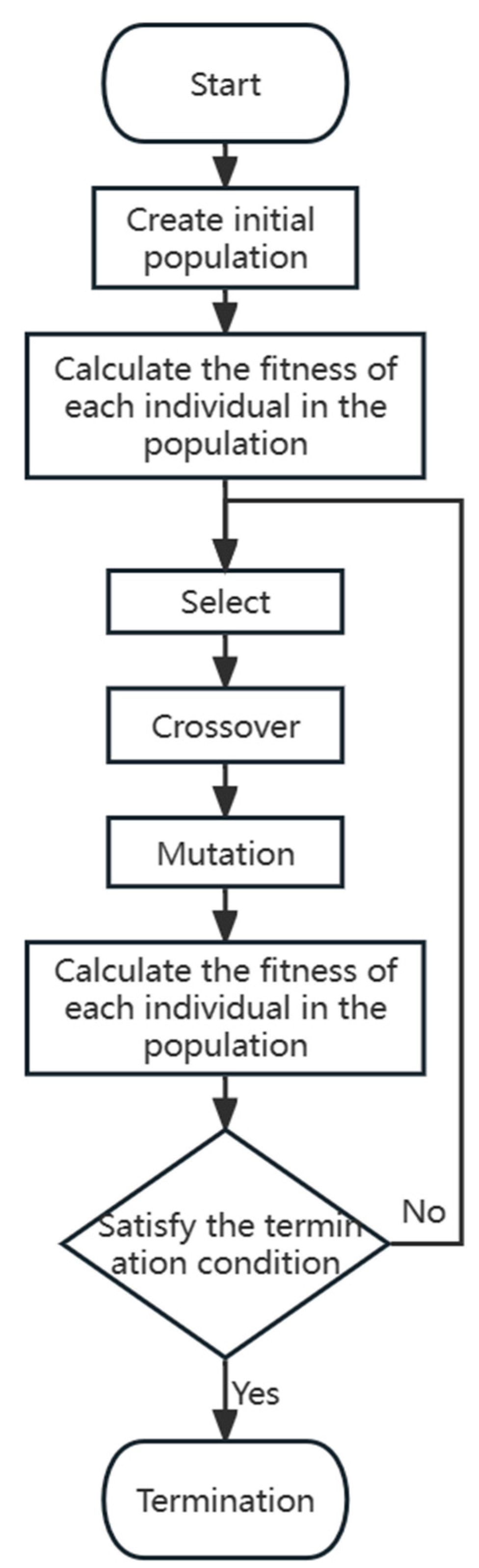
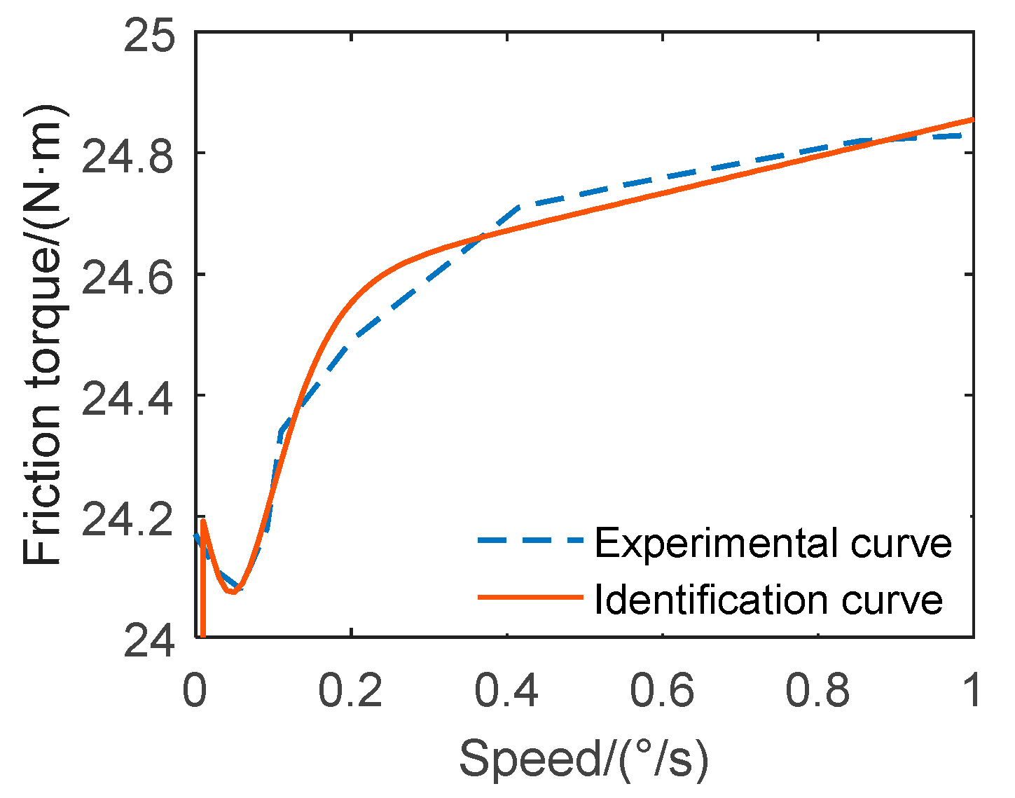
3.2. Identification of Friction Model Parameters

The formula for calculating the frictional torque of a continuous rotary motor system is:
T f = Δ P D m
where, Δ P is the differential pressure between the oil inlet and outlet at constant motor speed (MPa) and T f is the friction torque value (N·m).
A continuous rotary motor friction data collection experiment was carried out to run the motor at a series of constant angular speeds, eliminating the effect of rotational inertia. Ten sets of different input constant angular speeds were collected at 8 MPa oil pressure θ ˙ and the corresponding motor oil inlet and outlet pressure difference Δ P to obtain the friction torque value corresponding to the current speed.
The structure of the friction model is known according to the expression of the friction moment, and the parameters to be identified are k1, k2, k3, k4, k5, k6, and the model is non-linear. In order to improve the recognition accuracy of the friction model, a heuristic algorithm, genetic algorithm, is used to recognize the model parameters.
The fitness function is used to assess an individual’s ability to adapt to the environment. The new individuals generated during the iterative process have different levels of quality, and the individual fitness value determines whether the individual can participate in the next iteration. The problem solved in this paper is to identify the parameters of the friction model on the premise that the friction torque and the corresponding angular velocity data are available, and the smaller the fitting error, the better the individual is.
A quadratic performance optimization index is adopted as the objective function of the identification model.
J = min k i , i = 1 , 2 , , 6 ( T F T f ) 2
where, TF is the model-identified friction moment value.
The selection operation relates to the diversity of individuals in the offspring of the population, and the probability of an individual being selected during the selection process is related to its fitness value. In this paper, the roulette wheel method is used to match the weighting coefficients based on the different fitness of the offspring. The formula is as follows:
P i = F i i = 1 m F i
where, m is the number of individuals counted and F i is the individual fitness value.
When the crossover probability is large, the number of iterations can be reduced to increase the speed, but this may affect the diversity of the offspring population. Therefore, to ensure population diversity while increasing search ability, the value of the crossover probability is determined by the number of iterations, and the formula is as follows:
P c = P c 0 P c s t e p t P c > P c min P c = P c min P c P c min
where, P c 0 is the initial crossover probability; P c s t e p is the process crossover probability step; t is the current number of iterations; and P c min is the minimum crossover probability.
The variation operation is an auxiliary operation to improve the local search ability, find the optimal solution and accelerate the reaching; it can also help the crossover operation for global search, but the variation operator can also be degraded by taking values improperly. Therefore, this paper adopts a gradual increase in the variation rate, with the formula:
P m = P m 0 + P m s t e p t P m < P m max P m = P m max P m P m max
where, P m 0 is the initial variation probability; P m 0 is the variation rate increase step; t is the current number of iterations; and P m max is the maximum variation probability.
Accordingly, the parameter setting and refinement process of the genetic algorithm is as follows, which is shown in Figure 3.
(Step 1) Initialization of parameters, initial population N = 60, maximum number of iterations G = 100, number of chromosomes C = 6, crossover probability Pc = 0.9, variation probability Pm = 0.1, and iteration counter t = 0;
(Step 2) Calculate the fitness value of individuals in the population according to the objective function until i reaches the population size;
(Step 3) Apply the selection operator to the population, solving Step 2 for individuals with high fitness to be inherited directly to the next generation or matched with different weighting factors;
(Step 4) Two parent chromosomes are crossed over, thus generating new individuals with a certain probability of being superior to the parent and expanding the global search capability.
(Step 5) A change in the value of a gene of an individual during the mutation operation, thus generating a new individual, improving the local search capability and avoiding premature reaching of the algorithm;
(Step 6) If the algorithm meets the maximum fitness requirement, output the optimal parameters; otherwise, repeat Steps 2–5 until the maximum number of iterations is reached.
In order to reduce the randomness of the genetic algorithm search, the identification process is repeated several times, and the average value is finally taken as the final result of the continuous friction model identification. The exact parameter values obtained from the identification are shown in the Table 1 below.
The values of the identified parameters are brought into Equation (8) to obtain the final accurate friction model for the continuous rotary motor as follows:
T F = 24.26 ( tan h ( 12.77 q ˙ ) tan h ( 468.3 q ˙ ) ) + 24.55 tan h ( 12.34 q ˙ ) + 0.3057 q ˙
The values of the parameters of the friction model were identified by a genetic algorithm to determine the relationship between friction torque and angular velocity. Due to the limited number of samples collected, further experiments are required to verify the authenticity of the friction model. The estimated output values of the friction model are used to determine whether the model can be used as the actual friction model for the motor. A comparison of the friction torque curve obtained from the algorithm and the experimental sample points is shown in Figure 4 below.
The sampling points used in the Figure 4 are shown in Table 2 below.
From Figure 4, it can be observed that the output torque values of the identified friction model are able to converge well to the experimental torque values, and the maximum friction torque error value does not exceed 0.1 N·m. It is therefore used as the actual friction model for the motor system.

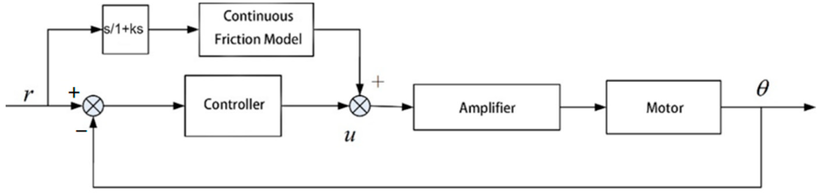
3.3. Friction Compensation

Friction in continuous rotary motors exists mainly between the top of the blade and the inner surface of the stator, between the blade end face and the end cap, and between the blade and the blade slot. Due to the friction torque causing system instability, steady-state errors and creep, appropriate friction compensation strategies are required to accurately estimate and compensate for frictional disturbances.
This paper uses a feedforward compensation method based on a continuous friction model, which is simple and easy to implement compared to the adaptive friction compensation scheme. By using this section to build a continuous friction model that describes the friction characteristics of the system, the non-linear frictional disturbances generated by the motor during low-speed operation or speed reversal are reduced. There are two options for feedforward friction compensation, either by adding a friction compensation signal to the control signal to offset the disturbance, or by superimposing a torque compensation on the motor output torque, and after a comparative analysis, this paper uses the signal input to offset the effect of frictional disturbance, as shown in Figure 5.

4. Sliding Mode Variable Structure Controller Based on Improved Power Reaching Law

4.1. Reaching Laws

Sliding mode variable structure controllers are a type of variable structure control theory where the system “structure” changes with time as a switching property and has strong robustness. The reaching law is designed to control the quality of motion of the system as the point of motion moves from space toward the surface of the sliding mode, while the sliding mode design can only accelerate the performance of the system as the point of motion reaches the sliding mode region and gradually converges to equilibrium. The quality of the entire transition process is determined by both components, and improving the performance of the reaching phase also requires attention.
The use of reaching law-based design methods can meet the needs of both reaching and sliding mode motion; therefore, the continuous improvement of reaching laws is of great research importance. The general reaching law is a commonly used control method and is expressed as follows:
s ˙ = ε sgn ( s ) f ( s )
where, ε > 0 ,   f ( 0 ) = 0 , when, s 0 s f ( s ) > 0 .
Varying the f ( s ) function, different forms of reaching laws can be derived, as shown in Table 3.
In Table 3, s ˙ is the reaching law; s is the slide mode surface; k ,   ε is the reaching law parameter; x is the system state quantity; and sgn is the symbolic for the sign function. These reaching laws all satisfy the stability conditions of s s ˙ < 0 . If the Lyapunov function V ( x ) = s 2 / 2 ,   s 0 is chosen to determine stability, the control system is stable and exists.
For the isokinetic reaching law, the time for the system state quantity to reach the sliding mode surface t * = s 0 / k and s 0 is a function of the initial moment at the slide mode surface. Therefore, an appropriate increase in k can accelerate the reaching speed, but too large a value of k can increase the chattering phenomenon.
For the exponential reaching law, the system arrives at the slide mode surface at t * = [ ln ( s 0 k + ε ) / ε ] / k , so increasing the value of k and decreasing the value of ε can regulate the reaching rate.
For the power reaching law, the integral is shifted to find the time required to reach t * = s 0 1 α ( 1 α ) k , and the change in control gain is achieved by adjusting a and k.
For the variable speed reaching law, when the system state variable x is large, it is jointly controlled by ε | x | ; when the system state variable x tends to zero, the control effect is equivalent to the equal speed reaching law.

4.2. Application of Reaching Laws

Presence of non-linear systems:
x ( n ) ( t ) = f ( x ,   t ) + b u ( t )
where, f ( x ,   t ) is the continuous bounded function and u ( t ) is the input function.
System tracking error is as follows:
e = x x d = [ e e ˙ e ( n 1 ) ] T
where, x d is the system tracking signal.
Selection of switching functions:
s ( x ) = i = 1 n c i e ( i 1 )
According to the Rouse stability criterion, so that all the roots of s ( x ) = 0 lie in the left half-plane of the s-plane, the selection of ci is as follows:
s ˙ ( x ) = c n e ( n ) + i = 1 n 1 c i e ( i ) = e ( n ) + i = 1 n 1 c i e ( i )
As an example of a reaching law control method that causes the system to form a sliding mode, the control law is designed as follows:
s ˙ ( x ) = e ( n ) + i = 1 n 1 c i e ( i ) = slaw u ( t ) = slaw i = 1 n 1 c i e ( i ) f ( x ,   t ) + x d ( n )
where slaw is the reaching law.

4.3. Improving the Power Reaching Law

In this paper, based on the power reaching law along with combining the advantages of the variable speed reaching law, we determine an improved power reaching law [13], and the mathematical expression is expressed as follows:
s ˙ = k 1 | s | α sgn ( s ) k 2 | x | | x | + 1 sgn ( s )
where, α , k 1 , k 2 is the reaching law parameter, k 1 > 0 ,   k 2 > 0 ,   α > 1 , and x is the system state variable.
At the initial moment of system state motion, when the variable speed term lim x k 2 | x | | x | + 1 = k 2 , the power term accelerates the system reaching process; when the system state enters into a sliding mode, the power term effect diminishes and the state quantity x in the variable speed term can adaptively adjust the chattering magnitude.
When the system tends to the equilibrium point:
lim x 0   k 2 | x | | x | + 1   x = lim x 0 ± k 2 | x | + 1 = ± k 2
Thus, improving the power reaching law allows the control system state to eventually converge to the equilibrium point, retaining the speed of the power reaching law and incorporating the advantages of the variable speed reaching law in adaptively regulating chattering.
Choosing the Lyapunov function V ( x ) = s 2 / 2 , substituting Equation (17) results as follows:
V ˙ = s s ˙ = s [ k 1 | s | α sgn ( s ) k 2 | x | | x | + 1 sgn ( s ) ] = k 1 | s | α + 1 k 2 | x | | x | + 1 | s | 0
Thus, the improved power reaching law satisfies the design accessibility condition for sliding mode variable structure controller systems.
Assuming the initial state of the system s ( x ) > 0 , then:
d s d t = k 1 s α k 2 | x | | x | + 1
Points awarded for:
s ( 0 ) 0 d s k 1 s α k 2 | x | | x | + 1 = 0 t   d t s ( 0 ) 0 d s k 1 s α
Shifting the terms and collating results in:
t s ( 0 ) 1 α k 1 ( 1 α )
The above equation shows that the control system has finite time reachability in the initial state of s ( x ) > 0 . The same can be proved for s ( x ) < 0 .
The motor state control equation is shown below.
{ x ˙ 1 = x 2 x ˙ 2 = x 3 x ˙ 3 = f ( x 2 ,   x 3 ) + b u
where, x 1 = θ is the continuous rotary motor angular position; x 2 = θ ˙ is the angular velocity; x 3 = θ ¨ is the angular acceleration, f ( x 2 ,   x 3 ) = 5852 x 2 30 x 3 ; and u is the control input.
Defining the slide mode surface s is as follows:
s = c 1 e + c 2 e ˙ + e ¨
where, c1, c2 is the sliding mode gain, c 1 > 0 ,   c 2 > 0 ; e is the motor tracking error, defined as follows:
{ e = r x d e ˙ = r ˙ x ˙ d e ¨ = r ¨ x ¨ d
where, r is the desired position signal, x d is the position tracking signal, and x d = θ .
Deriving the above equation and importing Equation (28) yields:
s ˙ = c 1 e ˙ + c 2 e ¨ + e = c 1 e ˙ + c 2 e ¨ + r x ˙ 3 = c 1 e ˙ + c 2 e ¨ + r f ( x 2 ,   x 3 ) b u
Combining Equation (22), a sliding mode variable structure control law based on a modified power reaching law for a continuous rotary motor system is obtained as follows:
u = 1 / b ( c 1 e ˙ + c 2 e ¨ + r f ( x 2 ,   x 3 ) + k 1 | s | α sgn ( s ) + k 2 | x 1 | | x 1 | + 1 sgn ( s ) )
The sliding mode variable structure composite controller built is shown in Figure 6.

5. Simulations

5.1. Determination of System Modal Parameters

The sliding mode variable structure composite controller requires parameter tuning in order to improve control performance and quality, based on an empirical approach to improve the parameters of the power reaching law and the sliding mode surface.
Firstly, the values of c1 and c2 are determined empirically. In order to ensure that the system movement point can quickly converge to the sliding mode surface without large steady-state errors, the value of c is not too large; the values of k1 and k2 are slightly smaller to reduce the steady-state errors and to meet the tracking performance of the system; the value of α is fine-tuned from the initial value to avoid overshooting. After several simulations, the values of the parameter variables of the sliding mode variable structure controller in this paper are as follows:
c 1 = 80 ,   c 2 = 60 ,   k 1 = 30 ,   k 2 = 10 ,   α = 1.1

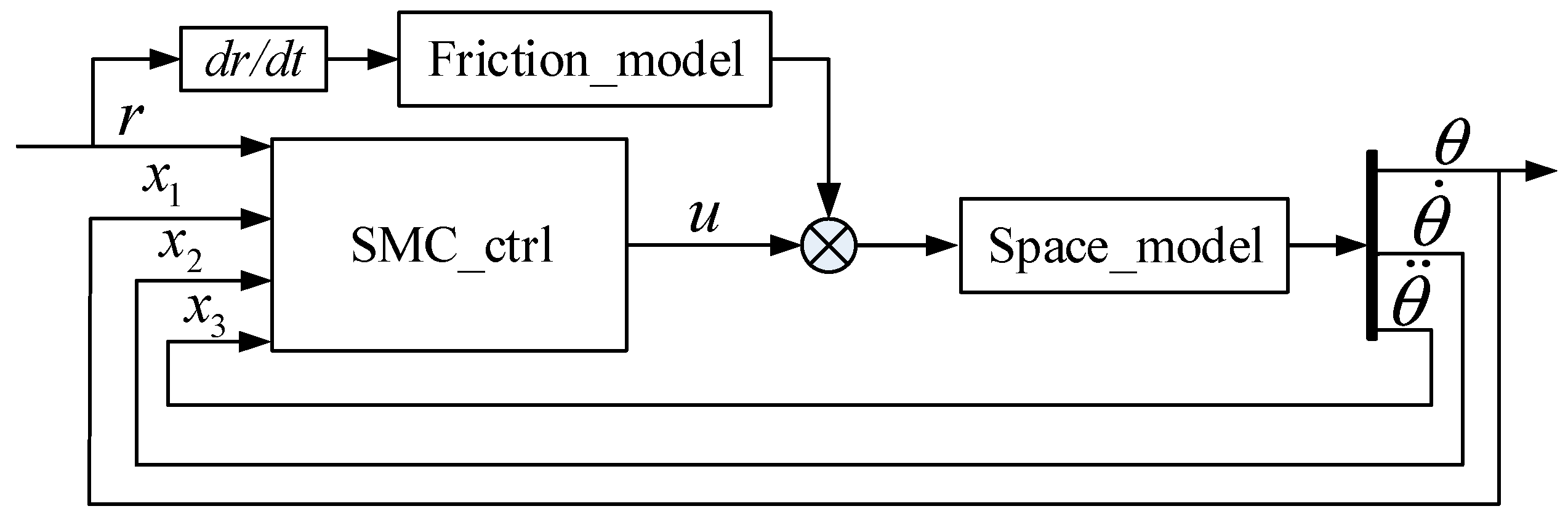
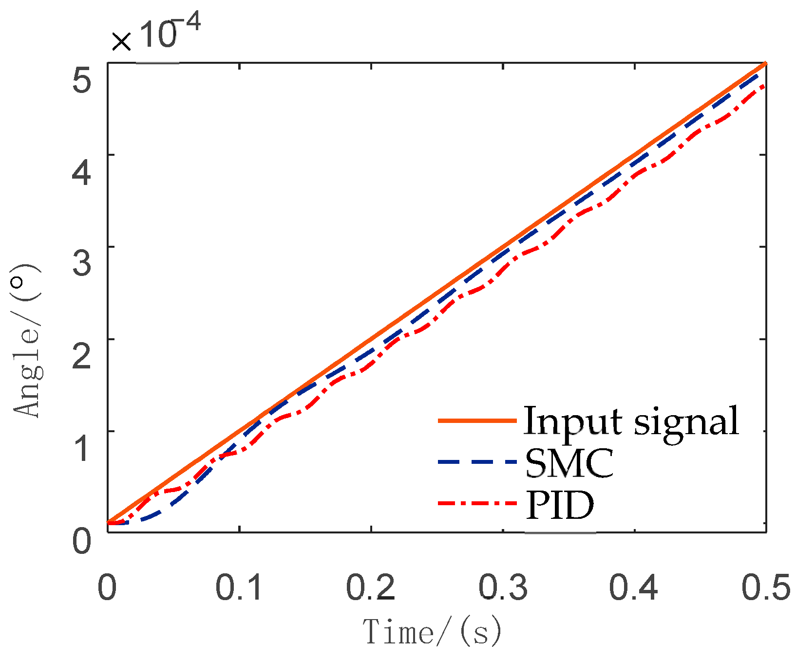
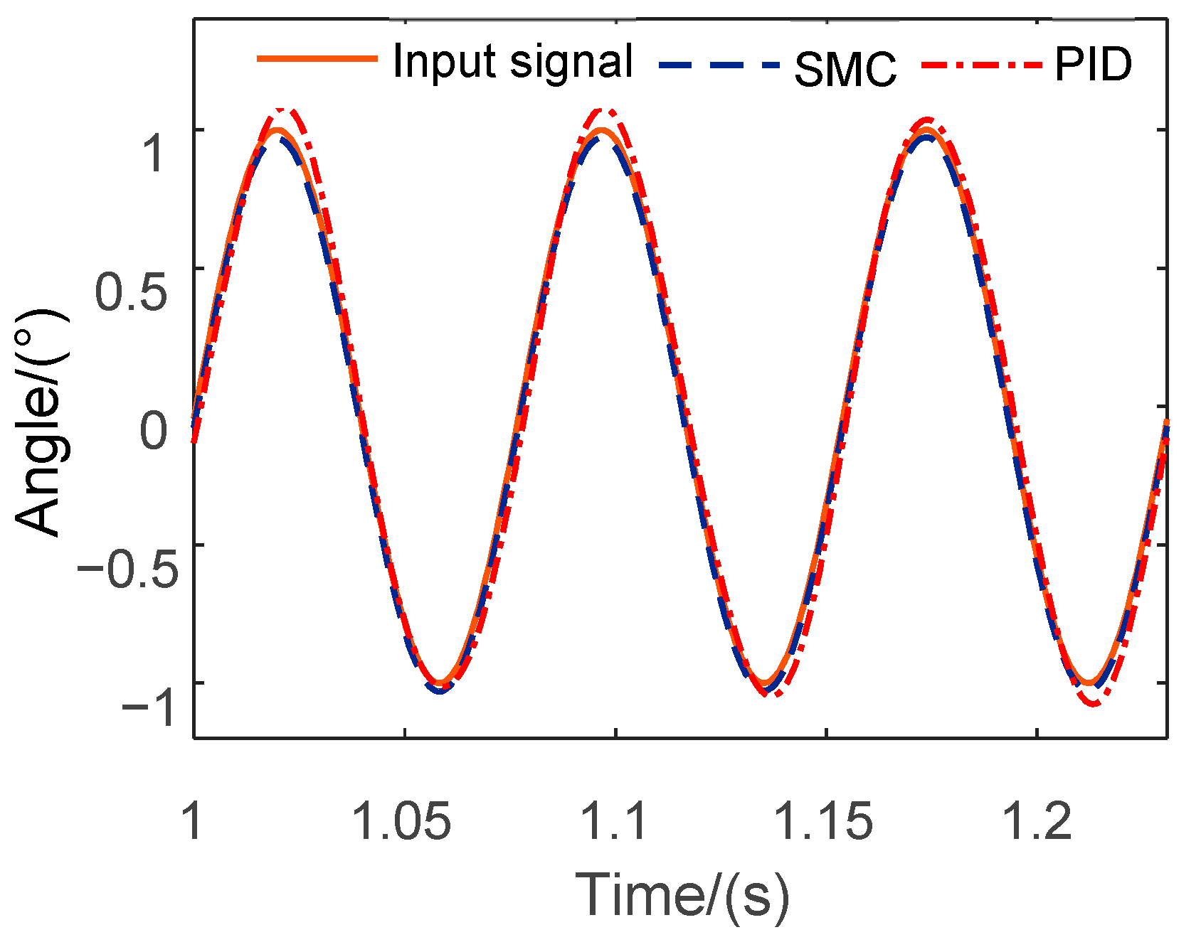
5.2. Simulink Simulation

In order to verify the above parameter tuning results, a composite controller is built in the Simulink environment based on the principle of a sliding mode variable structure controller, which is based on an improved power reaching law and a friction feedforward compensation scheme, and the S-function module is used to write the controller and the controlled system model program.
In order to verify the low-speed tracking performance of the sliding mode variable structure composite controller, a slope signal of 0.001°/s was used as the input signal to obtain a simulation comparison between the sliding mode variable structure composite controller and the PID controller, as shown in Figure 7.
As can be seen from the graph, the sliding mode variable structure composite controller based on the improved power reaching law has a slightly slower response than the PID controller, but has better low-speed tracking and a small steady-state error when it tends to stabilize, with no significant error fluctuations. The ramp signal simulation results show that both controllers do not show system creep and meet the low-speed performance requirements.
Using a sinusoidal signal as the input command signal, the output comparison curves of the PID controller (P = 410, I = 30, D = 18.5) and the sliding mode variable structure composite controller were obtained. The dynamic response of the controller under sinusoidal excitation with an amplitude of 1° and a frequency of 13 to 16 Hz is shown in Figure 8, Figure 9, Figure 10 and Figure 11.
By simulating the continuous rotary motor system under a sinusoidal signal with an amplitude of 1° and a frequency of 13–16 Hz, the PID controller has serious problems of amplitude error and phase lag, and the amplitude error increases significantly with the increase in frequency. The sliding mode variable structure controller has a stronger tracking capability than the PID controller, but with the increase in frequency, the phase lag increases and the amplitude begins to decay. The specific simulation data of the two controllers are shown in Table 4 and Table 5.
In summary, based on the double-ten indicators of amplitude error of less than 10% and phase error of less than 10°, under the role of PID controller, the phase error does not change significantly with the increase of sinusoidal signal frequency, but the amplitude of the output curve increases continuously, limited by the amplitude error, its sinusoidal response frequency by up to 13 Hz. While under the role of sliding mode variable structure composite controller, with the sinusoidal signal input under the action of the sliding mode variable structure composite controller and with the increase of the frequency of the sinusoidal signal input, its amplitude error and phase error intensify, and its highest tracking frequency can reach 15 Hz, which can indicate that the sliding mode variable structure composite controller is better than the PID controller in the control performance.

6. Conclusions

In this paper, a sliding mode variable structure complex controller based on a modified power reaching law is designed for a continuous rotary motor electro-hydraulic position servo system based on the principles of friction compensation and variable structure control. A continuous friction model is introduced, a genetic algorithm is used for parameter identification, and a feedforward compensation method based on the friction model is determined; the advantages of the power reaching law and the variable speed reaching law are combined, and a control method based on the improved power reaching law is proposed, and the motor system state variable x is introduced to adjust the chattering size adaptively. Through Simulink simulation and PID controller analysis comparison, the composite controller can make the system frequency reach 15 Hz under the tracking accuracy and can cause the response speed to meet the double-ten index requirements.

Author Contributions

Conceptualization, X.W. and Y.F.; methodology, X.W.; software, B.B.; validation, X.W., B.B. and Y.F.; formal analysis, B.B.; investigation, Y.F.; resources, X.W.; data curation, Y.F.; writing—original draft preparation, Y.F.; writing—review and editing, B.B.; visualization, B.B.; supervision, X.W.; project administration, X.W.; funding acquisition, X.W. All authors have read and agreed to the published version of the manuscript.

Funding

This research was funded by National Natural Science Foundation of China (Grant No. 51975164) and Outstanding youth of pyramid talent training project of Beijing University of Civil Engineering and Architecture (No: GDRC20220801) and 2023 Master’s Degree Innovation Project of Beijing University of Civil Engineering and Architecture (No: PG2023130).

Data Availability Statement

Not applicable.

Acknowledgments

This project was supported by National Natural Science Foundation of China (Grant No. 51975164) and Outstanding youth of pyramid talent training project of Beijing University of Civil Engineering and Architecture (No: GDRC20220801) and 2023 Master’s Degree Innovation Project of Beijing University of Civil Engineering and Architecture (No: PG2023130).

Conflicts of Interest

The authors declare no conflict of interest.

References

  1. Wang, X.J. Continuous Rotary Motor Electro-hydraulic Servo System Based on the Improved Repetitive Controller. J. Harbin Inst. Technol. 2010, 5, 731–734. [Google Scholar]
  2. Li, C.; Yan, Y.; Yang, Y. The Coordinate System Design and Implementation of the Spacecraft’s Attitude Simulation based on Five Axis Turntable. In Proceedings of the 2018 IEEE 3rd Advanced Information Technology, Electronic and Automation Control Conference, IAEAC, Chongqing, China, 12–14 October 2018; pp. 388–393. [Google Scholar]
  3. Feng, W. Research on the Control Performance of Large Displacement Continuous Rotary Electro-Hydraulic Servo Motor. Master’s Thesis, Harbin Institute of Technology, Harbin, China, 2011. Volume 3. pp. 1–26. [Google Scholar]
  4. Ma, Y. Application of QFT in the Control System of Continuous Rotary Electro-Hydraulic Servo Motor. Master’s Thesis, Harbin Institute of Technology, Harbin, China, 2008. Volume 6. pp. 7–11. [Google Scholar]
  5. Wensel, R.G.; Metcalfe, R.; Pothier, N.E.; Russell, B.G. O-ring Seal Studies for Space Shuttle Solid Rocket Booster Joints. Can. Aeronaut. Space J. 1988, 34, 204–212. [Google Scholar]
  6. Wei, L.J.; Han, S.X.; Xiong, Q.H.; Lv, L.; Duan, J. Effect of O-ring seal groove chamfer radius on sealing performance. Hydraul. Pneum. Seals 2016, 36, 72–75. [Google Scholar]
  7. Nikas, G.K.; Burridge, G.; Sayles, R.S. Modelling and Optimization of Rotary Vane Seals. ARCHIVE Proc. Inst. Mech. Eng. Part J J. Eng. Tribol. 2007, 221, 699–715. [Google Scholar] [CrossRef]
  8. Li, G.; Zhao, Q.; Li, Y.; Guo, B. Research on the sealing structure of electro-hydraulic servo oscillating motor. Lubr. Seal. 2015, 40, 9–13. [Google Scholar]
  9. Peng, Y.; Yu, X.; Tan, L. Research on friction characteristics and compensation of feed servo system based on improved Dahl model. Mod. Manuf. Eng. 2014, 114, 117–121. [Google Scholar]
  10. Simoni, L.; Beschi, M.; Visioli, A.; Åström, K.J. Inclusion of the Dwell Time Effect in the LuGre Friction Model. Mechatronics 2020, 66, 102345–102352. [Google Scholar] [CrossRef]
  11. Ni, F.; Liu, H.; Kai, D. Identification and compensation of GMS friction model based on speed observer. J. Electr. Mach. Control 2012, 16, 70–75. [Google Scholar]
  12. Li, Y.; Zeng, Y.; Pan, Q.; Jiang, X. Friction model of hydraulic cylinder considering pressure effect. J. Agric. Mach. 2020, 51, 418–426. [Google Scholar]
  13. Jiang, W.D.; Wang, H.T.; Zhang, S.H.; Ge, H.X.; Zhou, Z.D. Study of Buck converter sliding mode control method based on improved power reaching law. Electr. Drives 2021, 51, 58–63. [Google Scholar]
  14. Huo, A.; Zhang, S.; Wu, S. Sliding Mode Variable Structure Control of the Steerable Drilling Stabilized Platform Based on Disturbance Observer. J. Phys. Conf. Ser. 2021, 1894, 012033–012041. [Google Scholar] [CrossRef]
  15. Huang, X.P.; Ma, D.; Chen, X. Sliding Mode Variable Structure Control on Vienna Rectifier. In Proceedings of the 2020 Chinese Control and Decision Conference (CCDC), Hefei, China, 22–24 August 2020; IEEE: Piscataway, NJ, USA, 2020. [Google Scholar]
  16. Makkar, C.; Dixon, W.E.; Sawyer, W.G.; Hu, G. A New Continuously Differentiable Friction Model for Control Systems Design. In Proceedings of the 2005 IEEE/ASME International Conference on Advanced Intelligent Mechatronics, Monterey, CA, USA, 24–28 July 2005; pp. 600–605. [Google Scholar]
  17. Stotsky, A. Adaptive Estimation of the Engine Friction Torque. In Proceedings of the 44th IEEE Conference on Decision and Control, Seville, Spain, 15 December 2005; IEEE: Piscataway, NJ, USA, 2005. [Google Scholar]
  18. Stotsky, A.A. Data-driven algorithms for engine friction estimation. Proc. Inst. Mech. Eng. Part D J. Automob. Eng. 2006, 221, 901–909. [Google Scholar] [CrossRef]
  19. Slotinej, J.; Sastrys, S. Tracking Control of Non-Linear Systems Using Sliding Surfaces, with Application to Robot Manipulators. Int. J. Control 1983, 38, 465–492. [Google Scholar] [CrossRef] [Green Version]
  20. Qin, T.; Lu, D.L.; Zheng, G.J.; Lei, X.; Wang, T. Study on the sliding mode variable structure control of a stable aiming system based on PSO. Mod. Manuf. Technol. Equip. 2020, 56, 49–53. [Google Scholar]
  21. Rakhtala, S.M.; Ahmadi, M. Twisting control algorithm for the yaw and pitch tracking of a twin rotor UAV. In Proceedings of the 2015 2nd International Conference on Knowledge-Based Engineering and Innovation (KBEI), Tehran, Iran, 5–6 November 2015; pp. 276–284. [Google Scholar]
  22. Hou, H.; Yu, X.; Xu, L.; Rsetam, K.; Cao, Z. Finite-Time Continuous Terminal Sliding Mode Control of Servo Motor Systems. IEEE Trans. Ind. Electron. 2020, 67, 5647–5656. [Google Scholar] [CrossRef]
  23. Li, G.; Ding, Y.; Feng, Y.; Li, Y. AMESim simulation and energy control of hydraulic control system for direct drive electro-hydraulic servo die forging hammer. Int. J. Hydromechatronics 2019, 2, 203–225. [Google Scholar] [CrossRef]
  24. Kato, T.; Xu, Y.; Tanaka, T.; Shimazaki, K. Force control for ultraprecision hybrid electric-pneumatic vertical-positioning device. Int. J. Hydromechatronics 2021, 4, 185–201. [Google Scholar] [CrossRef]
Figure 1. Continuous rotary electro-hydraulic servo motor system.
Electronics 12 01447 g001
Figure 2. Block diagram of the transfer function of continuous rotary motor system.
Electronics 12 01447 g002
Figure 3. Genetic algorithm flow chart.
Electronics 12 01447 g003
Figure 4. Torque diagram of a continuous friction model.
Electronics 12 01447 g004
Figure 5. Frictional feedforward compensation diagram.
Electronics 12 01447 g005
Figure 6. Sliding mode variable structure composite controller.
Electronics 12 01447 g006
Figure 7. Comparison of slope response simulation.
Electronics 12 01447 g007
Figure 8. Dynamic response of the controller for a 13 Hz, 1° sinusoidal excitation.
Electronics 12 01447 g008
Figure 9. Dynamic response of the controller under sinusoidal excitation at 14 Hz and 1°.
Electronics 12 01447 g009
Figure 10. Dynamic response of the controller with sinusoidal excitation at 15 Hz and 1°.
Electronics 12 01447 g010
Figure 11. Dynamic response of the controller with sinusoidal excitation at 16 Hz and 1°.
Electronics 12 01447 g011
Table 1. Parameter identification results of friction model.
Model Parametersk1k2k3k4k5k6
Parameter values24.26−12.77−468.324.5512.340.3057
Table 2. Coordinates of sampling points.
X00.0270.0580.0920.110.20.4150.5620.8541
Y24.1724.1124.0824.1824.3424.4924.7124.7524.8224.83
Table 3. Comparison of the four reaching laws.
Reaching Law (Math.)Mathematical Expressions
Isokinetic reaching law s ˙ = ε sgn ( s ) ,   ε > 0
Exponential reaching law s ˙ = k s ε sgn ( s ) ,   k > 0 ,   ε > 0
Power reaching law s ˙ = k | s | α sgn ( s ) ,   k > 0 ,   1 > α > 0
Variable speed reaching law
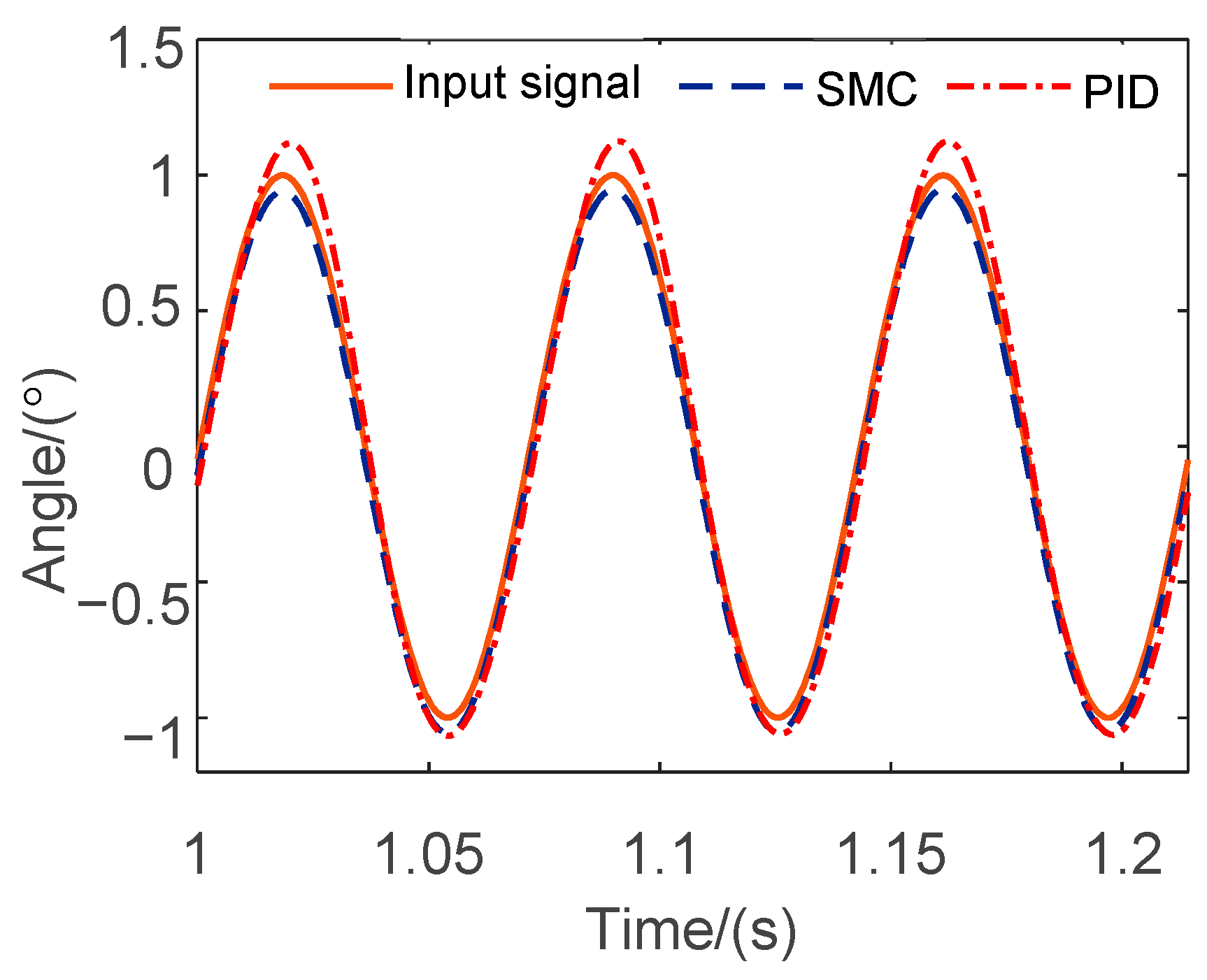
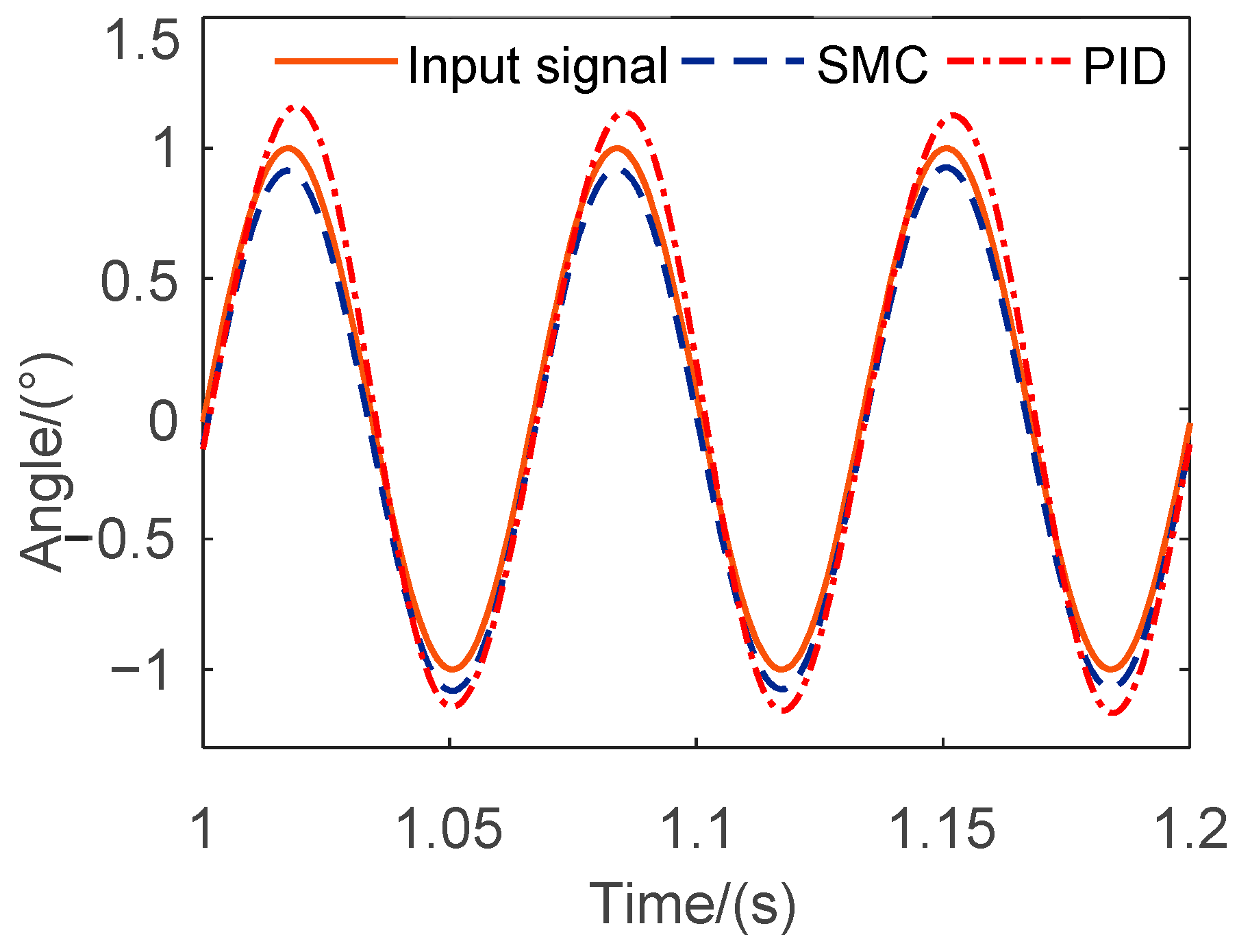
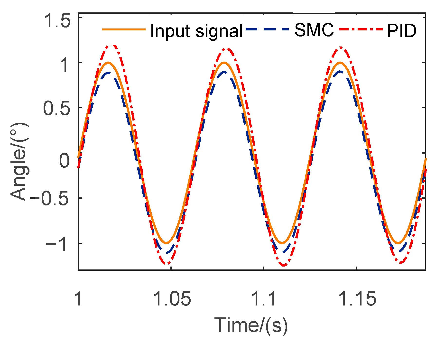
 s ˙ = ε | x | sgn ( s ) ,   ε > 0
Table 4. Comparison of sine response data.
Frequency/HzMagnitude Error/%Phase Error/°
PIDSMCPIDSMC
137.13.55.3811.872
1411.85.95.5423.526
1516.18.65.7584.858
162011.35.9376.333
Table 5. Comparison of slope response data.
PIDSMC
Scheme 55.0805 × 10−78.9490 × 10−8
MSE6.8143 × 10−72.9915 × 10⁻⁷
MAE2.1814 × 10−58.0668 × 10⁻⁶
RMSE2.2028 × 10−59.4552 × 10⁻⁶
MAPE0.00740.0078
Disclaimer/Publisher’s Note: The statements, opinions and data contained in all publications are solely those of the individual author(s) and contributor(s) and not of MDPI and/or the editor(s). MDPI and/or the editor(s) disclaim responsibility for any injury to people or property resulting from any ideas, methods, instructions or products referred to in the content.

