1. Introduction
In modern scientific research, an essential aspect is the rapid increase in the size of the arrays storing the experimental data, which can be further processed and analyzed at a later stage [
1,
2]. Different approaches to collecting (summarizing) the experimental data also provide different advantages and disadvantages in the further processing and analysis of the data [
3,
4]. Furthermore, the different nature of these data, such as their source and their inhomogeneity, makes the task of modeling them even more difficult. Therefore, the use of experimental datasets often requires preprocessing of the raw data, with the aim of easier access to these data, easier sharing of these data between different researchers, as well as easier postprocessing. This preliminary preparation of the data includes the selection of an appropriate format for storing these data, as well as a method of accessing the data in order to more easily access, retrieve, and analyze the aggregated information gathered in one centralized place. After the data have been preprocessed they can be converted and inserted (or imported in bulk) into a purpose-built local or remote database. From this database, information can be aggregated at a later stage and parts of it can be extracted for further analysis. This process leads to a change in the original format of the data, which is necessary to achieve a higher degree of uniformity of the data, so that it is possible to process them in the same way at a later stage. When centralized storage of the experimental data is used and access to it is carried out through a local or global network (e.g., an Ethernet or the internet), specialized data storage and delivery systems are used. These systems are usually database management systems (DBMS) [
5,
6,
7]. Different architectural models of multi-user systems based on dedicated database servers, which also provide additional possibilities for performing calculations and analysis of experimental data, have been presented in other scientific studies [
8,
9,
10].
A specific area that is oriented towards the analysis of the human decision-making process is still actively researched [
11,
12]. Methods based on artificial intelligence are mainly used, which are also widely discussed in various scientific studies [
13]. Through these methods, various processes are modeled [
14,
15], various experimental results are analyzed [
16], and various essential characteristics of the participating subjects are investigated [
17]. Many aspects of these methods, which are related to specific decision-making tasks based on visual stimuli, but which have only two possible responses, are also discussed in various scientific publications [
18,
19]. The goal is to study and analyze specific processes accompanying the decision-making process itself in humans [
20,
21]. Multiple approaches are also explored to determine the influence of decision time on decision accuracy in specifically used visual tasks (visual stimuli) [
22,
23]. Numerous approaches using neural networks have been developed for this purpose [
24,
25]. Through them, the generated experimental data are processed, after conducting the relevant sessions with the participants [
26], after which the decision-making processes are analyzed [
27,
28]. All these studies discuss the importance of the data processing methods. Specific data models and technologies are used to access them, such as relational databases and web services, object-relational, and object-oriented [
4]. In addition, various technologies and software methods have been used to access these data [
29,
30], as well as SQL servers for databases and web services [
8].
Various aspects and results of a specific study related to decision-making when visualizing visual tasks (stimuli) are presented in detail in [
9,
13,
31]. This research is oriented towards behavioral experiments and was conducted with real participants. The visual task stimuli are visualized on a computer display. The goal is that the participant should determine the direction of movement of the stimulus dots, left or right, respectively, by very quickly moving the gaze in the corresponding direction from the center of the computer display. This center is designated as the primary position in which the participant’s gaze should be fixed at the beginning of the experimental session. The gaze shift should be to the left or to the right end zone of the computer display on which the corresponding stimulus is displayed, respectively. At this point, the participant can press a mouse button to instruct the visualization software to display the next stimulus in the series of generated visual stimuli. The purpose of this experiment is to summarize and analyze the data related to the human perception and the movement of the human eyes when visualizing, analyzing, and solving visual tasks such as visual stimuli.
Each experimental session represented a visualization of preset sequences of stimuli. Each stimulus contained 100 frames, and each frame contained 50 points. Depending on the defined coherence of the points, each point changed its coordinates in a different way (i.e., its location relative to the other points). If the stimulus coherence parameter had a value of 100 (in percentages), then all points changed their coordinates synchronously in a certain direction. If this parameter had a value of 0 (also in percentages), then the points changed their coordinates randomly, both on the screen and relative to each other. Another parameter that was adjusted was the displacement of the set of dots relative to the center of the computer display. The values of this parameter varied between 20 and 140 (in pixels) and were distributed exactly in 7 levels (across 20 pixels each). An experimental condition is called a variant and contains a specific set of parameters and values of those parameters. Each variant was repeated exactly 10 times during one experimental session. One experimental session consisted of sequential visualization of 140 stimuli, with a total duration not exceeding 10 min. Each stimulus was actually a recognition task, in the case of the direction of movement of a set of dots on a computer display [
31,
32].
According to the type of movement of the dots, 4 types of stimuli were used, respectively combined, flicker, motion, and static. The static stimuli contained only 1 frame with 50 points, and the coordinates of these points did not change. In the other types of stimuli, the coordinates of dots were changed according to a predetermined rule, for example, all dots changed their location at the same distance and in a certain direction, or all dots were rotated by a certain angle relative to the center of the screen. In the combined type of stimuli, the movement of the dots depended on the direction of their orientation. In the flicker type of stimuli, the motion of the dots depended on their current position [
22]. The goal of the participant was to recognize the direction of motion of the dots, which was implemented in the corresponding visual task stimulus. The information for each stimulus was stored in a binary file with the extension “bin”, which had a specific structure and naming convention: the type of movement of the points, type of orientation of the points, distance of displacement of the points from the center of aperture, and variant number. The parameters that were essential for each stimulus were: coherence, direction, and speed of movement of points, number of frames in which one dot was displayed, total number of frames for the corresponding stimulus, coordinates, and the colors of the points in each frame. Stimuli were generated in advance, but presented in random order [
31].
The main part of the analyzed data was generated by a specific hardware device—a saccade sensor (Jazz novo eye tracking system, Ober Consulting Sp. Z o.o.). This device stores information about the eye movements of a particular subject at a sampling rate of 1000 Hz. The generated values are initially stored in a file with a specific file structure (and “jazz” extension) from which the data can be exported at a later stage to other files with flat text format [
31]. These data may include: aperture center calibration information, eye position information (horizontal and vertical in degrees relative to the viewing angle), a screen sensor signal depending on whether there is currently on the computer display visual stimulus or not, audio signal from a microphone with a frequency of 8000 Hz, as well as additional metadata about the experimental environment [
4,
22]. Other files (with the extension “dat”) store information about the order of presentation of the stimuli for each experimental session, as well as the main characteristics of the corresponding stimuli. These files also store the participants’ responses to the respective tasks (stimuli). These files are further processed and the information from them is aggregated, stored, and can be retrieved in various ways presented in [
4,
8]. These data can be exported from the database to external files in various formats as per user/researcher requirements.
All information from the conducted experiments was stored in a centralized database named
mvsemdb and contained 7 tables: “Participants”, “Stimuli”, “Frames”, “Dots”, “Sessions”, “Movements”, and “Experiments”. More detailed information about the structure of the
mvsemdb database is presented in [
4].
Table 1 shows a brief description of the purpose of each of the tables included in the
mvsemdb database.
In order to access the data in the
mvsemdb database, it was necessary that the corresponding user had created a login with at least the privilege to read data (
dbreader). Since this approach required the creation of multiple logins on the database server for more users, a specialized web service (
mvsemws) was developed for easier sharing of these data, which is presented in detail in [
8]. Web services provide opportunities through different technologies and approaches to reuse the same functionalities or data, which in turn can be sent to calling modules (applications and/or websites) and in different structural formats [
33,
34]. When using web services, this process is carried out both independently and very efficiently. Therefore, through this approach, functional and easily scalable software systems can be built by integrating multiple applications providing their functionality as web services in the form of web methods [
35,
36].
The
mvsemws web service provides five web methods. Each of these methods retrieves (and provides to the caller) a subset of the data in the
mvsemdb database. This web service is available on the internet at:
http://194.141.86.222/mvsemws/MvsemWebService.asmx (accessed on 30 November 2022). The technology for creating this web service (and its web methods), as well as the ways to use it, are presented in detail in [
8].
Table 2 shows a brief description of the purpose of each of the web methods provided by the
mvsemws web service.
More detailed information about the web methods, their input parameters, their speed of execution, as well as the main advantages and disadvantages of their use, is presented in [
8].
The subject of the present study is the presentation of a software product developed by the authors (named “SimulationCenter”), which, first, allows processing the heterogeneous information that is used in conducting the experimental sessions, and second, allows recreating the experimental sessions themselves. All data used during the experimental sessions were available (in the original format) and could be retrieved either from the centralized database—
mvsemdb or from the open access web service—
mvsemws. Then, these data could be stored in files and processed according to the research objectives. The software that we have developed and present in this article can convert, process, and visualize all types of data used during experimental sessions, and through this functionality it can accurately reproduce each experimental session. The formats used by the software are mainly of three types—plain text, xml, and a specific binary format used by client datasets [
9,
31]. The main advantage of using the xml format is that it is platform-independent, meaning that it is easily portable while being self-descriptive [
37]. Its main disadvantage is that the self-descriptive nature of the data multiplies the size of the xml files [
38]. When software stores data in binary form (used by client datasets), the volume of data is significantly smaller compared to that of the xml format, while binary data are loaded (buffered) and processed much faster in memory than data formatted with xml tags [
9].
The SimulationCenter application provides the possibility to process different types of “raw” data that are created beforehand (such as the stimulus files) or generated at a later stage during the experimental sessions (such as the files generated by the saccade sensor). Another important function of this application is the ability to convert all types of (heterogeneous) data from one format to another; thus, the application is also a powerful conversion module. This is possible because the software converts all types of data to a common binary format that it can process and convert back to the source format for each of the supported formats. After the application converts, i.e., reorganizes the data at a structural level and merges them, it can also export these data to other applications using the specific file formats that are supported. The most important function of the SimulationCenter application is the ability to recreate each experimental session by visualizing to the user both the stimuli themselves and the eye movements projected on the computer display. Various approaches described in detail in scientific publications were used for the development of the application [
39,
40]. In addition, various software development technologies and methods have been used, which are also widely discussed in the scientific literature [
41,
42]. From the point of view of software engineering, the creation of such software that provides functionalities for collecting, processing, summarizing, and analyzing experimental data, and such data collected from different and heterogeneous sources, is a serious problem [
43,
44]. The purpose of the present work was to test and analyze the main functions of the SimulationCenter application, as well as verify its effectiveness and functionality by conducting experimental tests, and then present the results of these tests.
2. Materials and Methods
In order to recreate the experimental sessions, the SimulationCenter application first needs to process and convert 3 different types of files from their original “raw” form to a form ready to be used by the application itself. These are the stimulus files, the files storing the audio signal from the microphone, and the files storing the eye movement information. We will also note that the processed audio files are merged at a later stage with the eye movement files. This is necessary to synchronize the two files, since the sample rate of the eye movement file is 1000 Hz, and the audio signal that the microphone recorded is 8000 Hz. In order to synchronize the data in a common file, it is necessary to match each sample from the eye movement file with eight samples from the audio file that was recorded by the microphone. In this section, we will introduce the steps to convert all these files. We will introduce the conversion of the stimulus files first.
The coordinates of all 5000 points of all 100 frames in one stimulus are stored in a binary file. These files have a specific file structure. This requires additional processing to extract the necessary information from these files. This information contains the coordinates of certain points distributed in certain frames (for each stimulus file).
Table 3 shows fragments of a stimulus file named: cl201.bin.
The following additional abbreviations are used in
Table 3: F—frame, P—point, X—X coordinate, Y—Y coordinate. Each stimulus file is 20,100 bytes in size. The last 100 bytes contain color information, one value for each of the 100 frames. The values for the colors are respectively 0—white, 1—black, 2—combined. The remaining 20,000 bytes store information about the X and Y coordinates at 5000 points (distributed at 50 points in 100 frames). The X and Y coordinates at each point are written in two 16-bit integer values, which correspond exactly to 2 bytes. Since the points are 5000, and for each of them both the X coordinate and the Y coordinate are stored, the total number of values that need to be stored is 5000 × 2 = 10,000. Since each value is written in a 16-bit number (2 bytes), all 10000 values will require exactly 20,000 bytes.
Table 1 also shows the hexadecimal equivalents of the coordinates of points 1 and 2 of frame 1, as well as point 50 of frame 100. One specific feature of the stimulus files is that in the first 10,000 bytes only the X coordinates of all 5000 points are stored, and in the next 10,000 bytes only the Y coordinates of all points are stored. In this way, the X coordinate of point 1 of frame 1 is “extracted” from bytes 0–1, respectively, and the Y coordinate from bytes 10,000–10,001. Similarly, the X coordinate at point 50 of frame 100 is “extracted” from bytes 9998–9999, respectively, and the Y coordinate from bytes 19,998 and 19,999, respectively. This way of storing the information about the coordinates of the points in the stimulus files is inconvenient to process (
Figure 1).
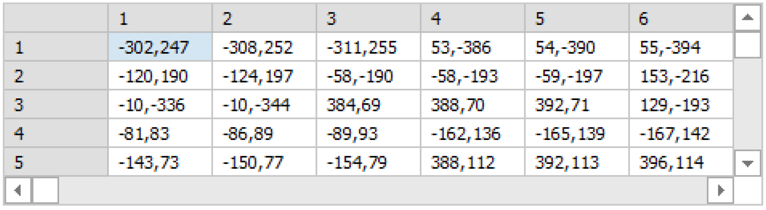
Therefore, in the presented ordinance of the coordinates of the points in a stimulus file, the software developed by us, first, converts into a two-dimensional matrix—PF (short for points by frames), which has a dimension of 50 rows per 100 columns (
Figure 2). Each cell of this matrix contains one TPoint element, which is a structure (packed record) containing two integer values, one for the X coordinates and one for the Y coordinate of a given point. Each column of the matrix corresponds to exactly one frame of a given stimulus, and each row contains the X and Y coordinates of each of a total of 50 points for the specified frame.
The PF matrix is transformative and is in fact an intermediate structure that stores the data on the coordinates of the points per frame (for a given stimulus) in a more convenient form for processing. However, for further processing of the information from the stimulus files, we converted a two-dimensional PF matrix into the “stimulus” relation, with the following analytical representation: stimulus = {ID, frame, point, Xcoord, Ycoord}, where the primary key ID contains unique values in the range from 1 to 5000 and corresponds to the index of a particular point of a frame in a particular stimulus. The values of the frame attribute change in the interval [1, 2, …, 100], as this is the total number of frames in each stimulus. The values of the point attribute change in the interval [1, 2, …, 50] and correspond to the point number in the current frame. The values X and Y, respectively, represent the coordinates of the current point of the current frame.
Figure 3 shows the “stimulus” relation after transformation of the PF matrix (for stimulus cl201.bin).
The ID attribute (which is the primary key) in the “stimulus” relation can be removed and the combination of the values of the frame and point attributes can be used instead. This combination of attribute values, as well as the ID attribute, fulfills the two conditions that must be met by a primary key in a relationship [
6]: (1) uniqueness—to ensure the uniqueness of each value of a given attribute (or combination of attribute values) and (2) minimality—neither of the two frame nor point attributes can be removed without violating the uniqueness condition. Removing either of the two frame or point attributes will duplicate the values in the other attribute, because for each point in a frame, the frame number is repeated exactly 50 times. On the other hand, for each frame (a total of 100 for each stimulus) the numbers of points from 1 to 50 are repeated. However, the combination of frame number and point number (frame, point) is unique for each of the states of the stimulus relation. The ID attribute will be used to more quickly index the points and frames in the dataset that stores the information for a particular stimulus. The values of this attribute guarantee the uniqueness of each point of each frame in each stimulus. From each value of the ID attribute, the corresponding frame number and the corresponding point number can be calculated. Since each frame is known to contain exactly 50 points, then for each ID (in the range from 1 to 5000) the values of the variables PointIndex and FrameIndex can be calculated as follows:
Remainder = ID mod 50; if (Remainder = 0): PointIndex = 50; FrameIndex = ID div 50;
if (Remainder > 0): PointIndex = Remainder; FrameIndex = (ID div 50) + 1;
The data organized in this way, containing the distribution of points by frames and the coordinates of these points, provide significant advantages in searching and filtering fragments of a stimulus or unidirectional extraction of coordinates of points distributed in frames when displaying a stimulus on the screen of the computer.
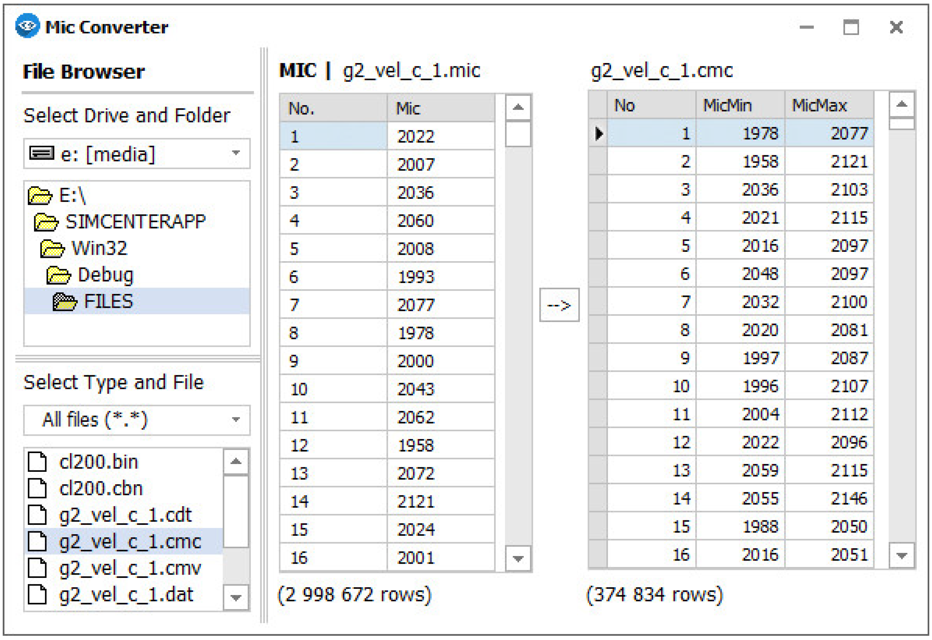
We will present the initial processing and conversion of the audio signal that is recorded by the microphone. All audio signal values that are stored by the microphone are saved in files with the extension “mic”. Since these files have a specific structure, they need to be further processed. The microphone records the sound signal with a frequency of 8000 Hz, which means that for 1 millisecond the microphone stores 8 values. However, these 8 values should correspond to only 1 value, which is stored by the saccade sensor, which, however, works with a sampling rate of 1000 Hz. This requires additional processing of the audio signal and its synchronization with the signal stored by the saccade sensor, which corresponds to the eye movement. For this purpose, an additional module called MicConverter was developed and integrated into the SimulationCenter application, which allows processing, converting, and synchronizing the microphone signal with the signal from the saccade sensor. An example session of working with the MicConverter module is shown in
Figure 4.
The MicConveter module converts the original binary format of the audio signal that was recorded by the microphone, then converts it to a pair of integer values, respectively “sample number” and “audio value for this sample (in decibels)”. In order to synchronize the two signals in duration, the first audio signal stored by the microphone and the second stored by the saccade sensor, it is necessary to match exactly 8 values of the audio signal for every value of the saccade sensor signal. To realize this, the MicConverter module divides the audio signal into segments, each segment containing exactly 8 values. These values (in decibels) overlap each other, thereby “merging” into a single discrete that has a corresponding minimum value (this is the lowest discrete value of the 8 considered) and maximum value (this is respectively the highest value of a discrete of the same 8 values in the corresponding segment). Thus, the processed microphone signal, containing an array of discrete signal value pairs, is actually an intermediate transform structure that the MicConverter module will use to generate the synchronized (reduced exactly 8 times) and converted audio signal.
For more convenient processing of the information from the audio signal (recorded by the microphone) and its synchronization with the signal recorded by the saccade sensor, the array containing the pairs of values “discrete”, “signal” in the relation “MicSignal” was converted. This relation has the following analytical representation: MicSignal = {No, MicMin, MicMax}, where No is the primary key and contains unique values that are identical to the index values of the values generated by the saccade sensor. The MicMin and MicMax values respectively contain the minimum and maximum value of the audio signal (in decibels) recorded by the microphone for the corresponding segment.
Figure 4 shows that the first 8 samples of the microphone signal form a single entry (with index 1) in the MicSignal relation. The corresponding minimum value in this 8-element segment is at a discrete with index 8, and the maximum value is at a discrete with index 7. From the next 8 values of the microphone signal, i.e., those contained in segment 2, a single entry (with index 2) is also formed in the MicSignal relation. In this segment, the corresponding minimum value is at a discrete with index 12, and the maximum value is at a discrete with index 14. It is observed that the original microphone signal contains exactly 2,998,672 values, and the converted signal contains 374,834 values, which is exactly 8 times less. This number of values will also uniquely and precisely match the number of values stored by the saccade sensor that is associated with eye movement information for the same experimental session. In this way, the data from the saccade sensor can be easily synchronized with the data from the audio signal that are recorded by the microphone. The audio signal is used for background noise analysis.
The process of merging the signal recorded by the saccade sensor (stores the eye movement information) and the signal recorded by the microphone (but already processed and converted) can be performed. For each session, the eye movement values generated by the saccade sensor are stored, as well as additional values generated by the application associated with the saccade sensor. The stored file contains for every 1 millisecond the values for the gaze deviation (i.e., their projection on the computer display), both the X coordinate and also the Y coordinate. In addition to these values, the index of the current discrete is also generated and stored, as well as an additional parameter indicating whether a stimulus is currently being visualized on the computer display or not. The eye movement values are calculated by the saccade sensor and represent the projection of the participant’s gaze onto the computer display at a certain moment. For every 1 millisecond (of the corresponding experimental session), the saccade sensor generates one pair of such values, and the application associated with the saccade sensor adds the other two automatically. The data are then exported from this application to a flat text file. Since an experimental session can last 10 min or more, the amount of the data that will be generated can be very large. For example, with a session duration of 10 min (which is equal to 600 s or 600,000 milliseconds), the amount of data that must be stored after converting the text file to structures with certain data types will be 600,000 multiplied by the number of bytes to store each value from the 4 generated ones, and for each one discrete. We note that for each set of 4 values generated by the saccade sensor and its associated application (for each sample), it is necessary to add the values from the microphone signal for the same sample (MicMin and MicMax). Since these signals are already synchronized, they can easily be combined into one, which is shown in
Figure 5.
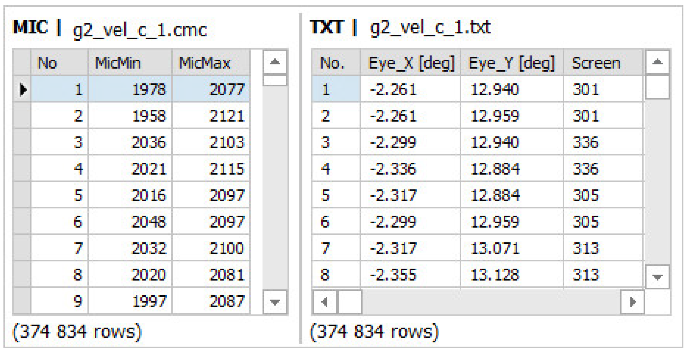
Handling the data from two structures that are different in data type, one of which contains string values, is inconvenient. It is necessary to convert the eye movement information data, which are currently of text type, to the corresponding base (structural) types. This conversion is done in parallel with the process of merging the eye movement data and the pairs of MicMin and MicMax values, which correspond to the minimum and maximum value of the audio signal for the corresponding segment, but extracted from the text file. The eye movement data are initially loaded and buffered into an array of strings whose elements are record type variables that hold 5 different values each. These values correspond to each field that is exported to the text file that stores the eye movement information. To join the two sets of records, the relation Movments = {No, EyeX, EyeY, Screen, MicMin, MicMax} was created. The first 4 fields correspond to the columns of the same name from a text file, and the last 2 fields correspond to the minimum and maximum value of the microphone signal for the current sample. In this relation, the “No” attribute actually represents a primary key and uniquely identifies each row of the formed record structure. The result of converting the text file containing the eye movement data and merging it with the microphone signal data is presented in
Figure 6.
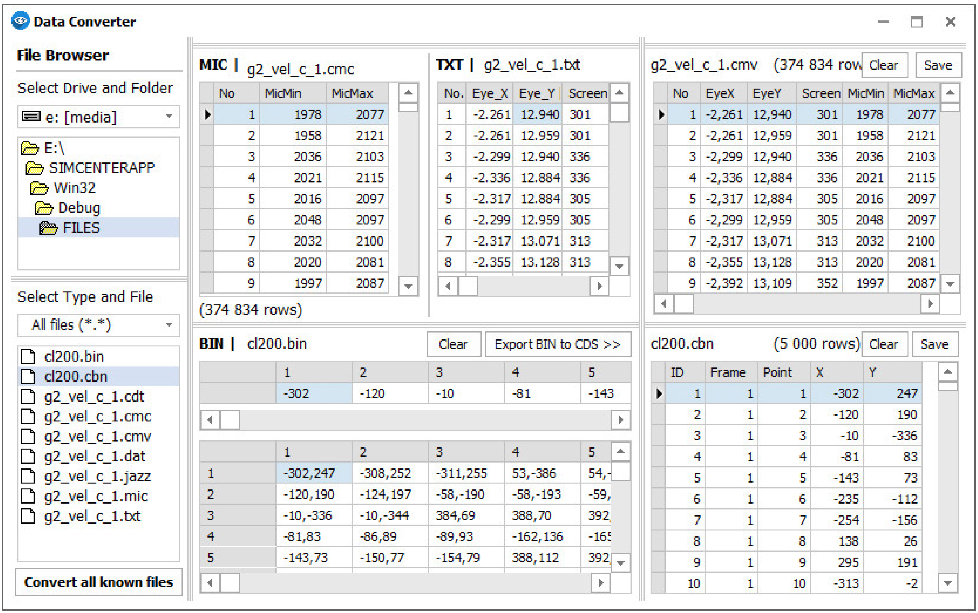
Figure 7 shows a working session with the data converter unit of the SimulationCenter application.
The data organized in this way already contain information about the index of the corresponding discrete, about the coordinates of the projection of the participant’s averted gaze on the computer display, about the visualization or not of a stimulus at the current moment, as well as about the minimum and maximum values generated by the microphone for the corresponding segment. This data format already provides significant advantages when playing back and analyzing complete experimental sessions, or when working with partial fragments of them.
It is important to note that when the data are of a character type, mathematical calculations cannot be performed with these data. Apart from the stimulus binaries, all other files, i.e., those generated by the saccade sensor and the associated software, are of a character type. Therefore, data preprocessing and conversion is necessary, as this will enable the data to be converted to the appropriate base types (e.g., integer, word, double, etc.). After converting the data to the corresponding base types, they can be analyzed and visualized in a convenient way.
3. Results
The subject of this research is the SimulationCenter application and its functionalities. This application was run on a 32-bit Win 10 OS with the following hardware configuration: AMD (R) Ryzen (TM) 3 5300U (up to 3.85 GHz, 4 MB cache, 4 core) processor, 8 GB RAM, and AMD Radeon (TM) Desktop Graphics Card.
Figure 8 shows a session with the main unit of the SimulationCenter application. The main module of this application provides capabilities for visualization of various types of data in an interactive mode. After selecting a stimulus file, it can be visualized frame by frame on a simulation display. This display has the same aspect ratio as the original computer display on which the real stimuli are visualized. This module also provides options for selecting a specific experimental session that can be interactively played within the application.
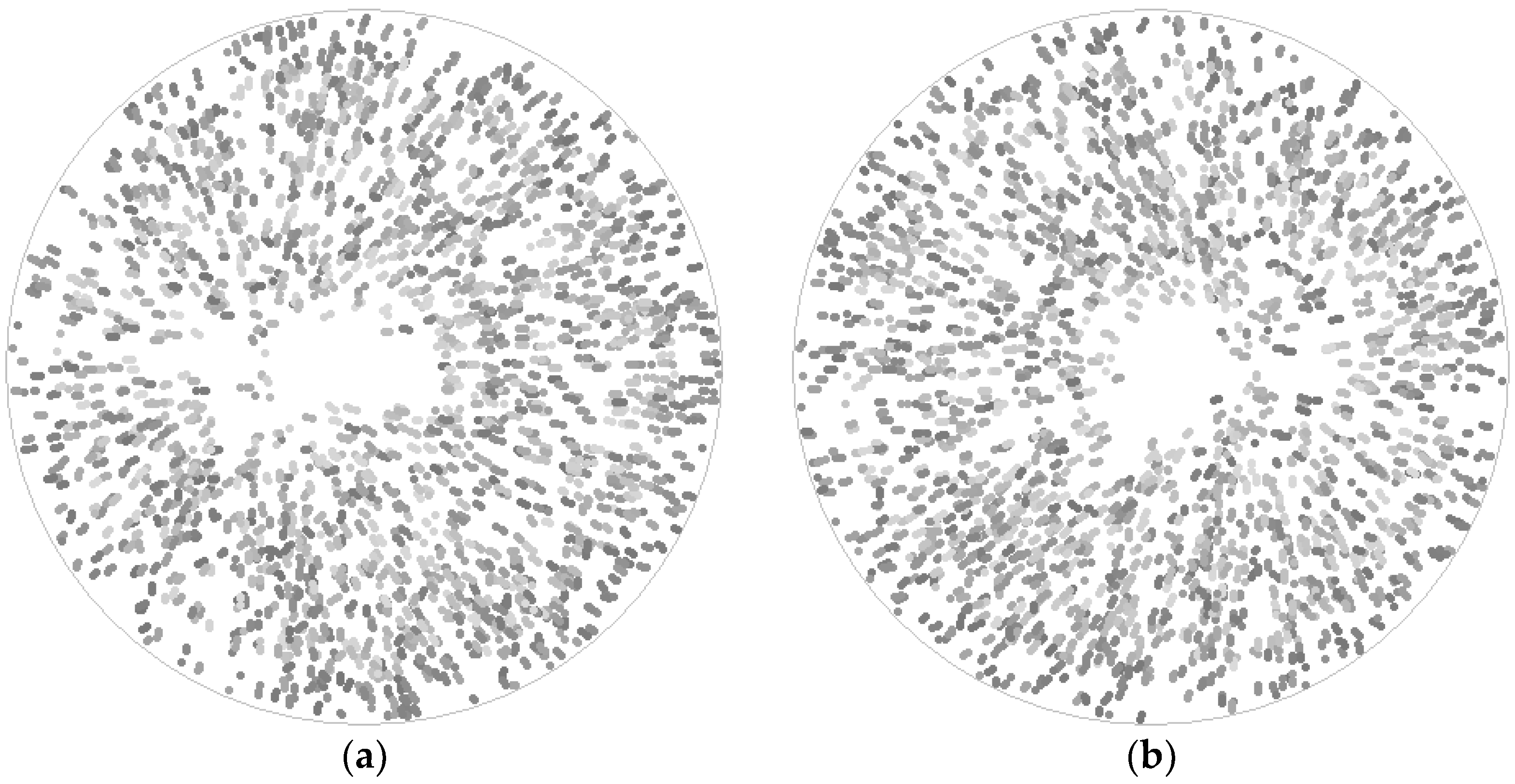
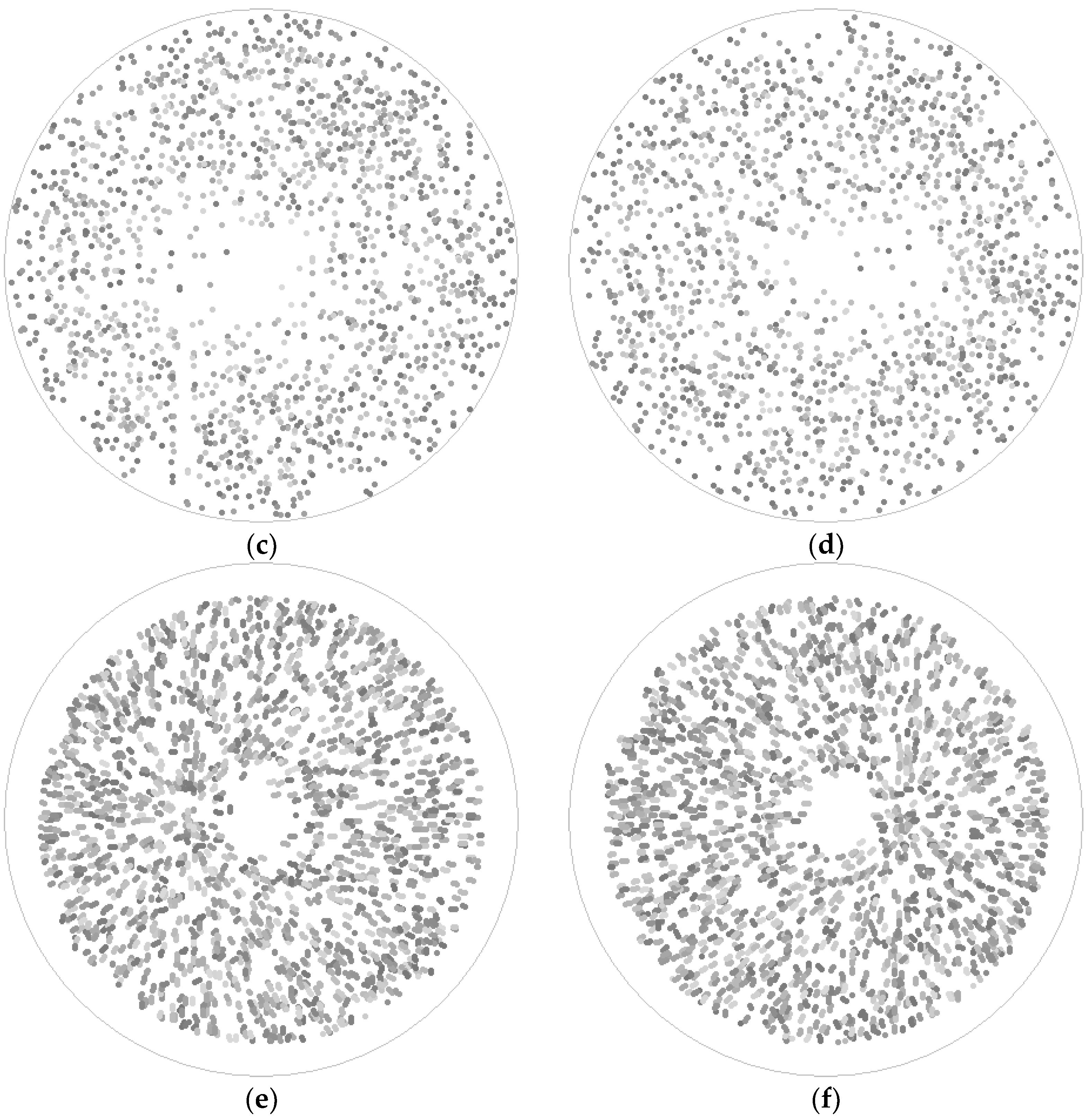
The first experiment with the SimulationCenter application that was done was to interactively visualize six stimuli using the built-in support for interactive visualization of stimuli. The application shows what the participant in the experiment saw during the experimental session itself. Interactive visualizations of these stimuli generated by the SimulationCenter application are shown in
Figure 9a–f.
The difference is in the place where the stimulus will be visualized. In the real experiment, this is the computer display in front of the participant himself, but in the present test, it was the computer display on which the main window of the SimulationCenter application was displayed. Six files were selected, respectively divided into pairs for each of the combined, flicker, and motion types. For each of the stimulus dot movement types, one leftward and one rightward dot movement were selected, respectively. The stimuli were selected so that their dots had the largest displacement from the center of the aperture, i.e., 140 pixels. Variant 9 was selected for all stimuli.
We note that after conducting this experiment, it was found that visualizing the stimuli frame by frame, although recreating what the participant in the experiment saw, could not create the sensation of movement of the set of dots. In fact, when previewing the stimuli, the application shows the frames one after the other but does not erase them. This way, the images shown in
Figure 9a–f were generated. This way of visualizing the stimuli shows how the set of points forms the displacement from the center of the aperture to the left or right depending on the currently visualized stimulus and the type of motion that is selected, respectively combined, motion or flicker.
The second experiment that was done with the SimulationCenter application was to test its functionality in terms of the possibility to reproduce, interactively, the eye movement process on the computer display by a participant in the experiment during the visualization of the stimuli. This can be recreated and visualized to the user/analyst using the application.
Figure 10 shows the eye movement visualization for an entire experimental session.
In order that the user/analyst determines how the participant’s eye movements were made over time, the application changes the color saturation of the graph by which it visualizes the gaze projection in the simulated computer display. Less saturated colors indicate projection coordinates in the earlier phases of the experimental session, and the darker tones indicate later moments of this process. We should also note that the user can simultaneously visualize both the eye movement and the corresponding stimulus.
The application provides functions of a group and summarizes data in an easy way. This provides an opportunity for these data to be more easily analyzed. In order to test this capability of the application, an analysis of the obtained results of the experiments was made from the point of view of the correct and incorrect answers given by the participants to the visual tasks. These visual tasks were based on stimuli for which two key parameters were defined, respectively, first according to the type of movement of the stimuli: combined, flicker, motion, and static, and second according to the size of displacement [
4,
8,
9]. The summary data are presented in
Table 4 and
Table 5.
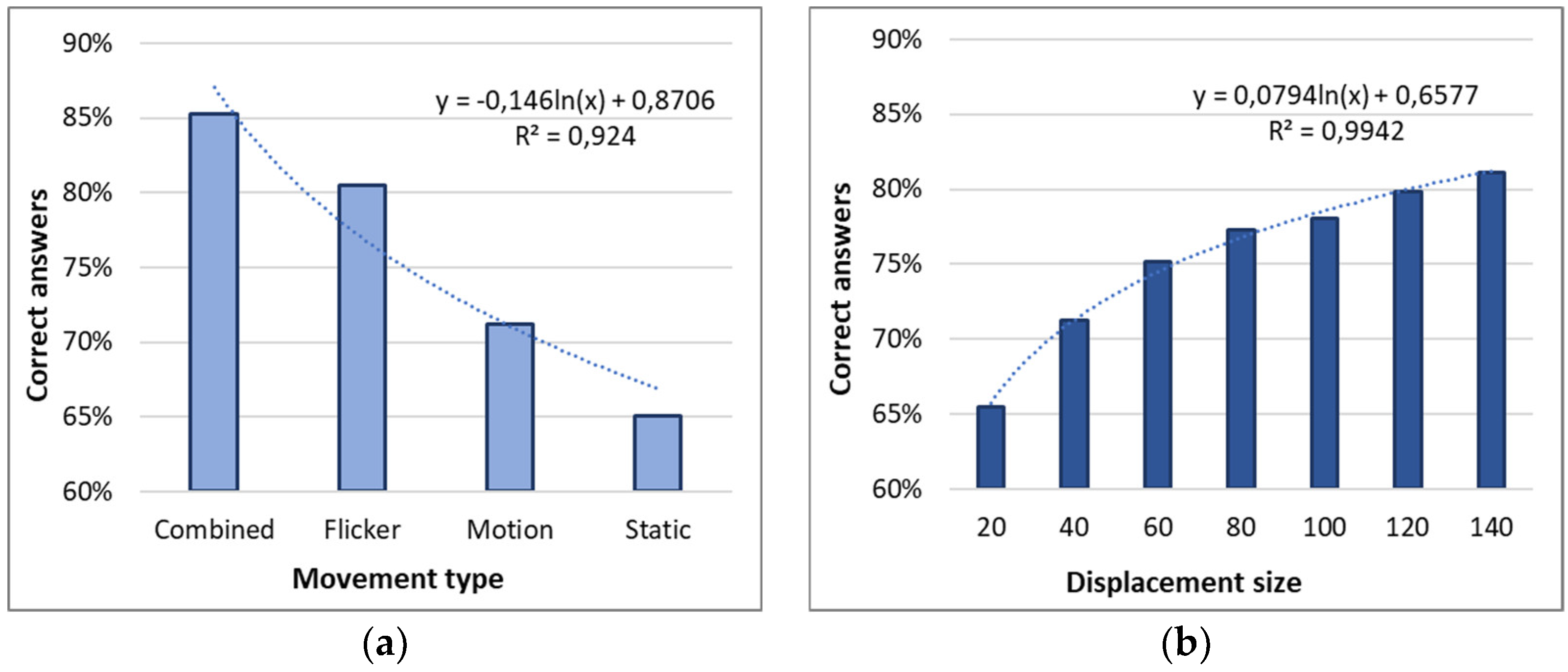
These data were analyzed with the goal of examining how the type of stimulus motion (i.e., combined, flicker, motion, and static) affects participants’ responses and how the size of the displacement affects the responses of the visual tasks but is summarized to all participants in the experiment. The graphs of these results are shown in
Figure 11a,b.
Table 4 and
Table 5 and the diagrams in
Figure 11a,b show that the type of movement of the stimuli has an impact on the number (percentage) of correctly solved visual tasks, with the best results obtained in the type of movement of the combined and flicker stimuli. In the motion type of the stimuli, given the complex dynamics of changing the locations and directions of the individual dots in the frames, it can also explain the difficulties that the participants had when making a decision in this type of motion. With the type of movement of the stimuli static, we note that the worst results were obtained, i.e., with this kind of stimulus movement, the information that the experimenters receive is as little as possible, since the dots are static and their positions do not change during visualization of the stimulus. On the other hand, the lack of dynamics of the points also leads to more difficult decision-making by the participants. Regarding the size of the displacement of the center of the set of dots from the center of the aperture, we can note that a tendency also stands out and it is the following: the number of correctly solved visual tasks depends on the size of the displacement. This is because the larger the displacement of the center of the set of dots from the center of the aperture, the more noticeable it is, and thus the participant makes a decision more easily. Because of this, the number of correctly recognized stimulus directions by participants (i.e., the number of correctly solved visual tasks) increased as the amount of displacement from the center of the set of dots relative to the center of the aperture increased. A detailed statistical analysis of the results is presented in [
9,
13,
31].
We will now perform another analysis on the same data, examining how the type of stimulus motion (i.e., combined, flicker, motion, and static) affects the participants’ decision times, and secondly how the displacement of the center of the cluster of points from the center of the aperture affected the decision time (summed) for all participants in the experiment. The graphs of these results are shown in
Figure 12a,b.
Table 4 and
Table 5 and the diagrams in
Figure 12a,b show that for the motion type of the stimuli, there was no clear trend in terms of the participants’ decision times. We note that in the combined flicker and static movements, the total decision-making time was comparable for all three types, which varied in the range from 3 h 45 min to 3 h 56 min. In contrast to these movements, with the movement of the motion stimuli, the reaction time (decision time by the participants) was significantly longer: it was 4 h 34 min, which was generalized for all experimental sessions. We can summarize that with motion stimuli, in addition to the longest decision-making time, at the same time the number of correctly recognized stimuli was significantly lower. Regarding the size of the displacement of the set of dots from the center of the aperture and the time to make a decision, we note that there was a clearly marked trend and it was the following: the time to make the decisions depended inversely on the size of the displacement of the set of dots from the center of the aperture. This can be explained by the fact that the greater the displacement of the set of dots from the center of the aperture, the more noticeable this displacement was and the corresponding decision could be made by the participant faster. Furthermore, as noted in the analysis of
Figure 11b, this displacement also resulted in a greater number of correctly solved visual tasks. We can summarize that the number (percentage) of correctly solved visual tasks was a function of the size of the displacement of the set of dots from the center of the aperture. Although the decision time decreased as the size of the displacement increased, the number of correct answers maintained an increasing trend.


