
Charging Behavior Analysis Based on Operation Data of Private BEV Customers in Beijing

Abstract
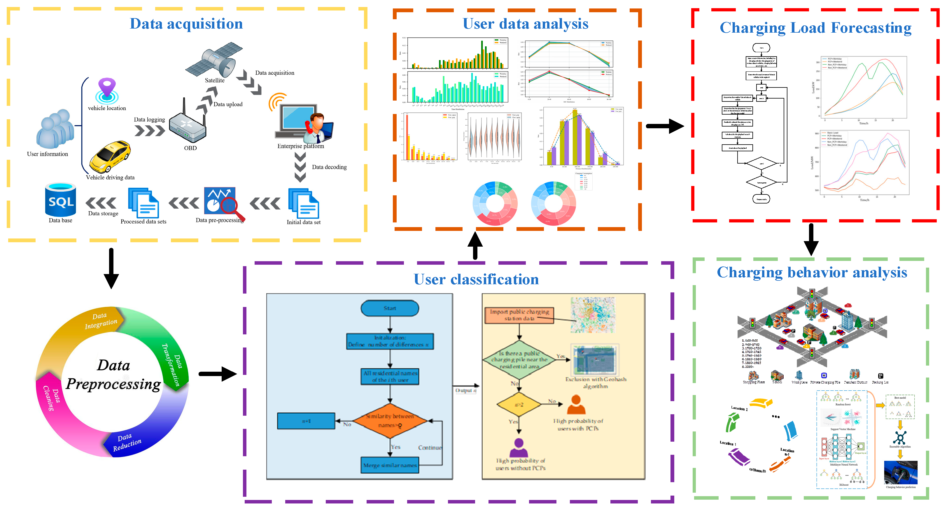
:1. Introduction
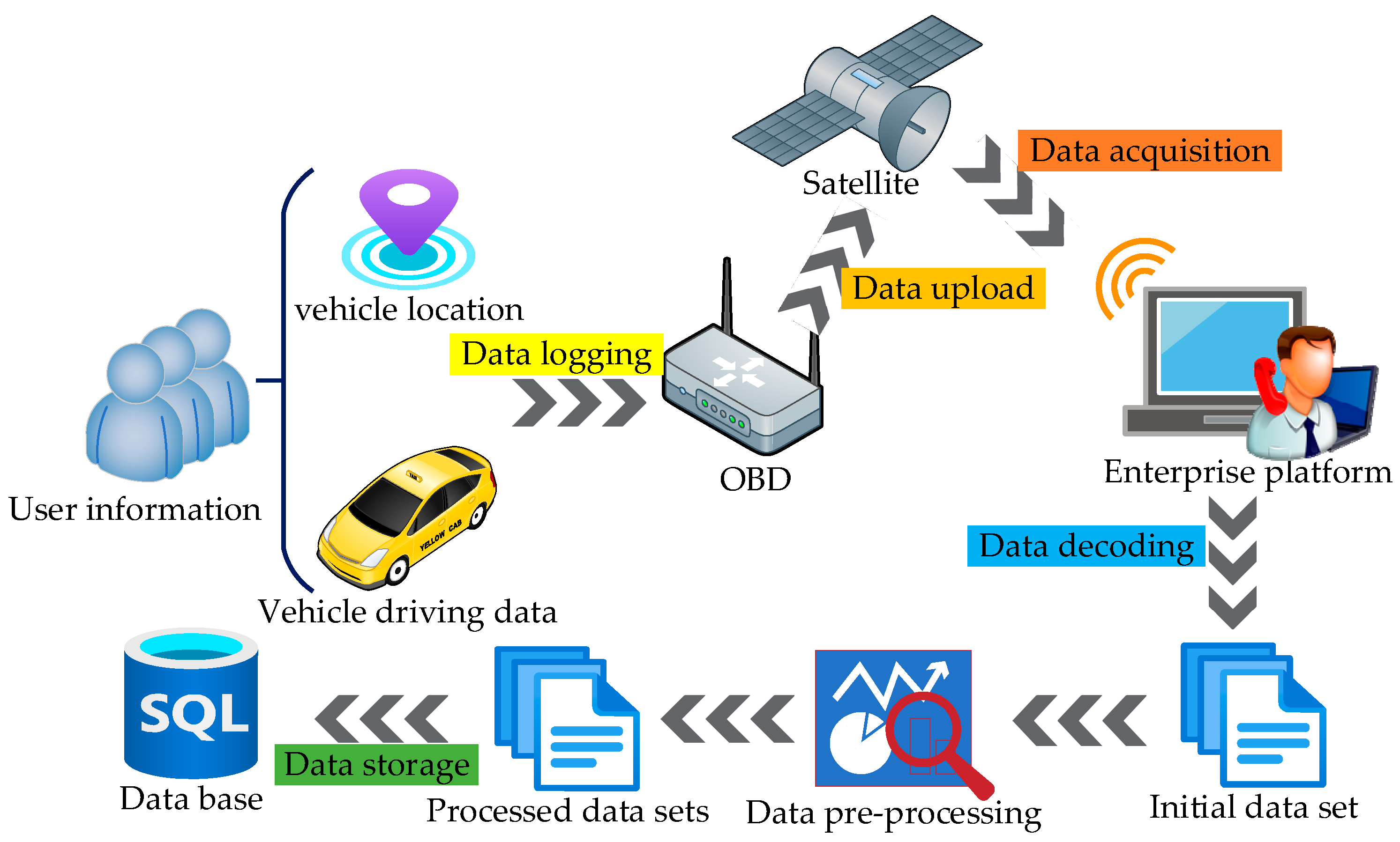
2. Data Collection and Processing
2.1. Data Sources
2.2. Data Preprocessing
2.3. Extraction of Charging Segments
- Extracting fragment for the first time
- Extracting fragment for the second time
3. User Classification of BEVs
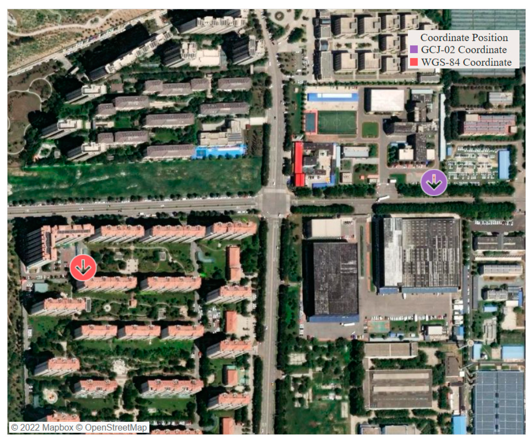
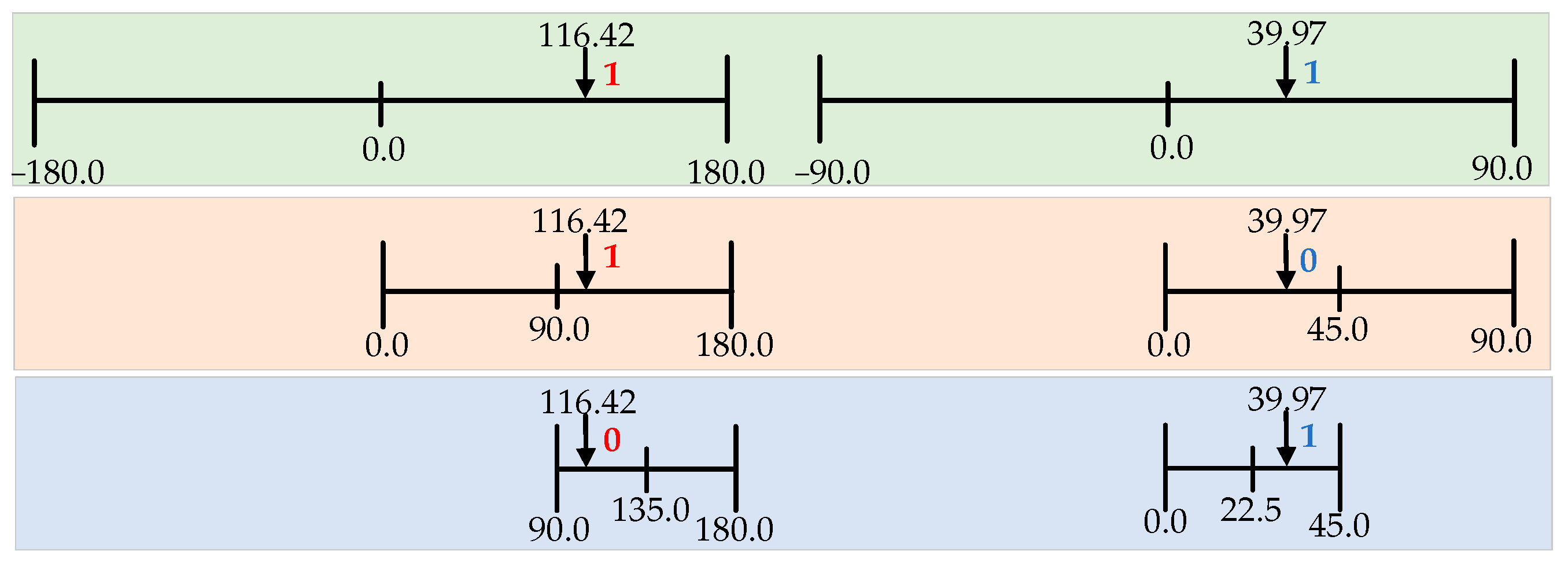
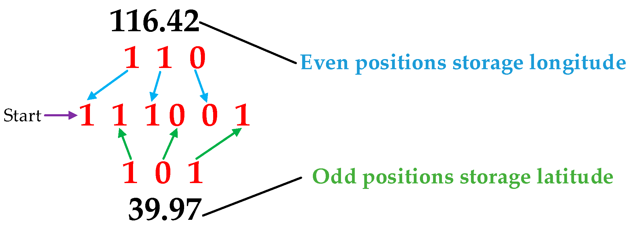
3.1. Coordinate System Transformation
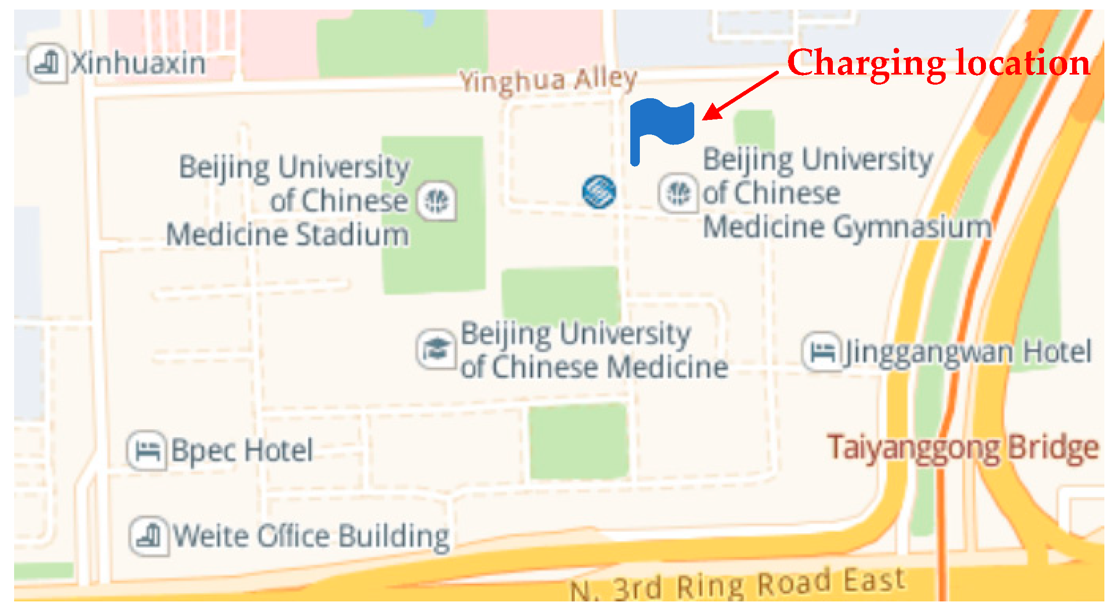
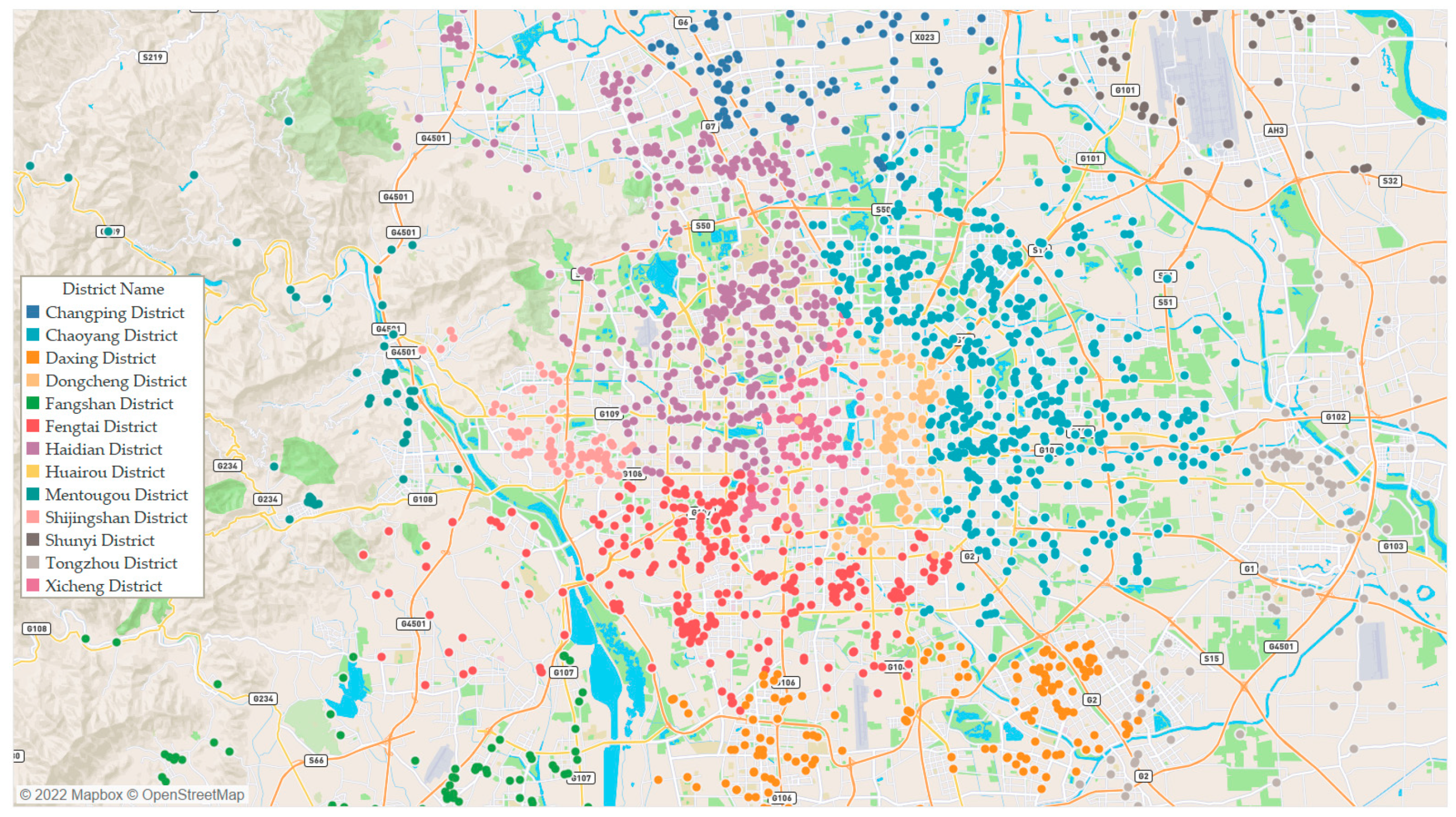
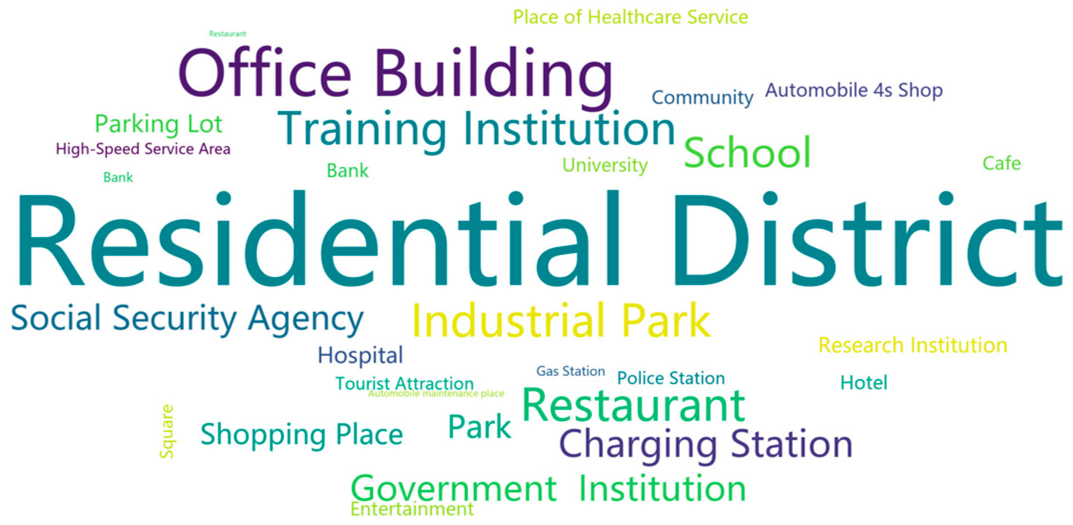
3.2. Inverse Geocoding
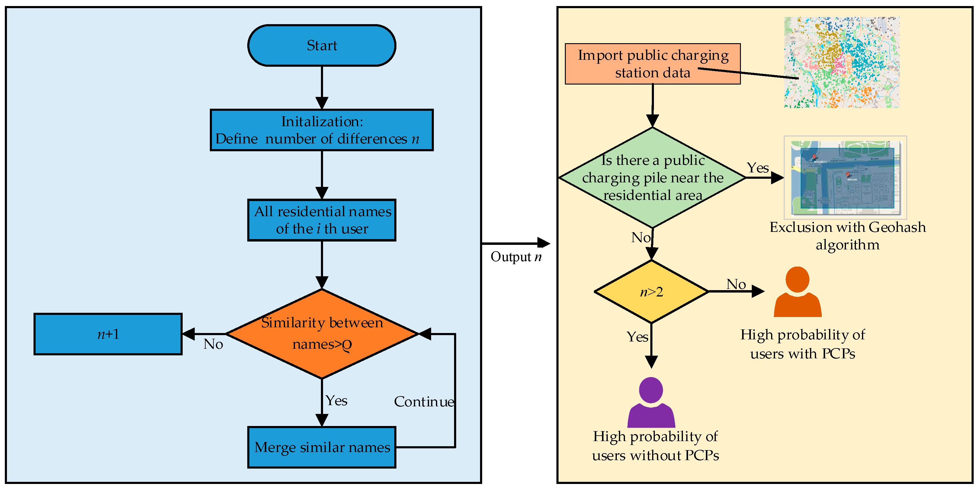
3.3. User Classification
3.3.1. First Screening
3.3.2. Second Screening
4. User Charging Behavior Analysis
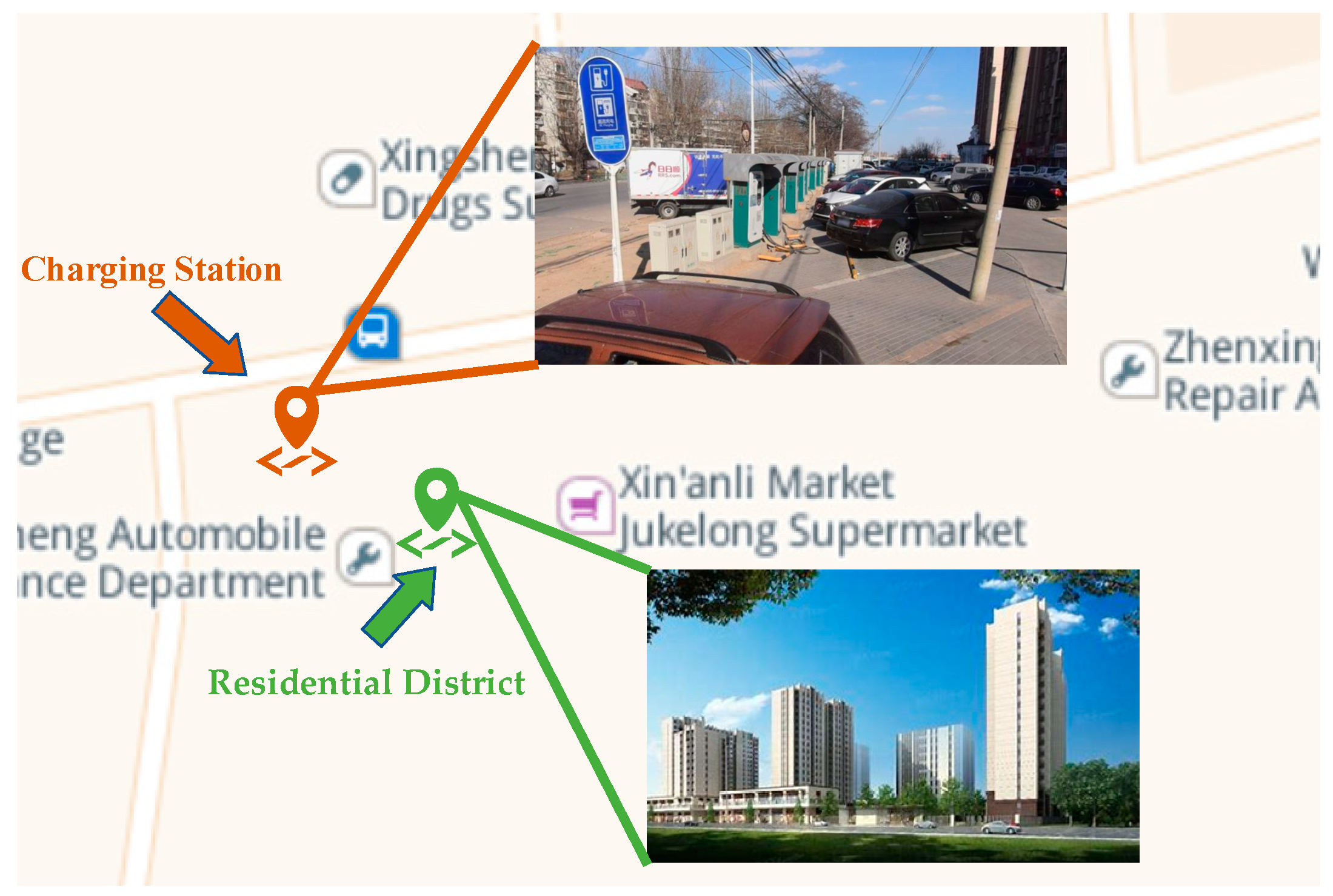
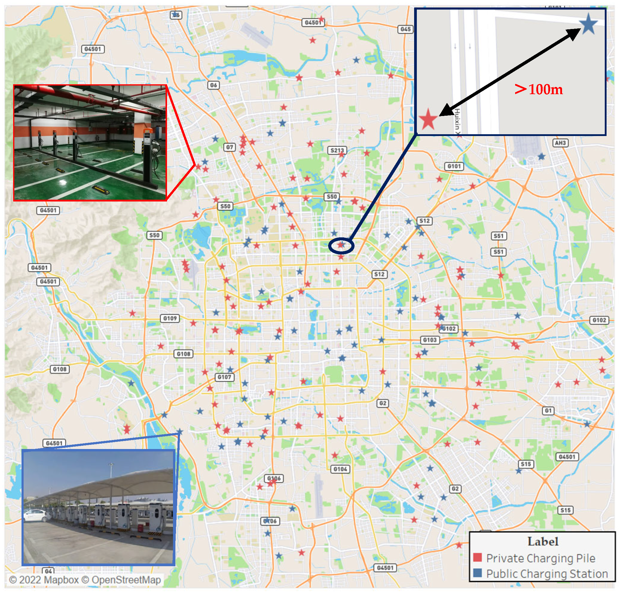
4.1. Charging Location Selection
4.2. Charging Behavior
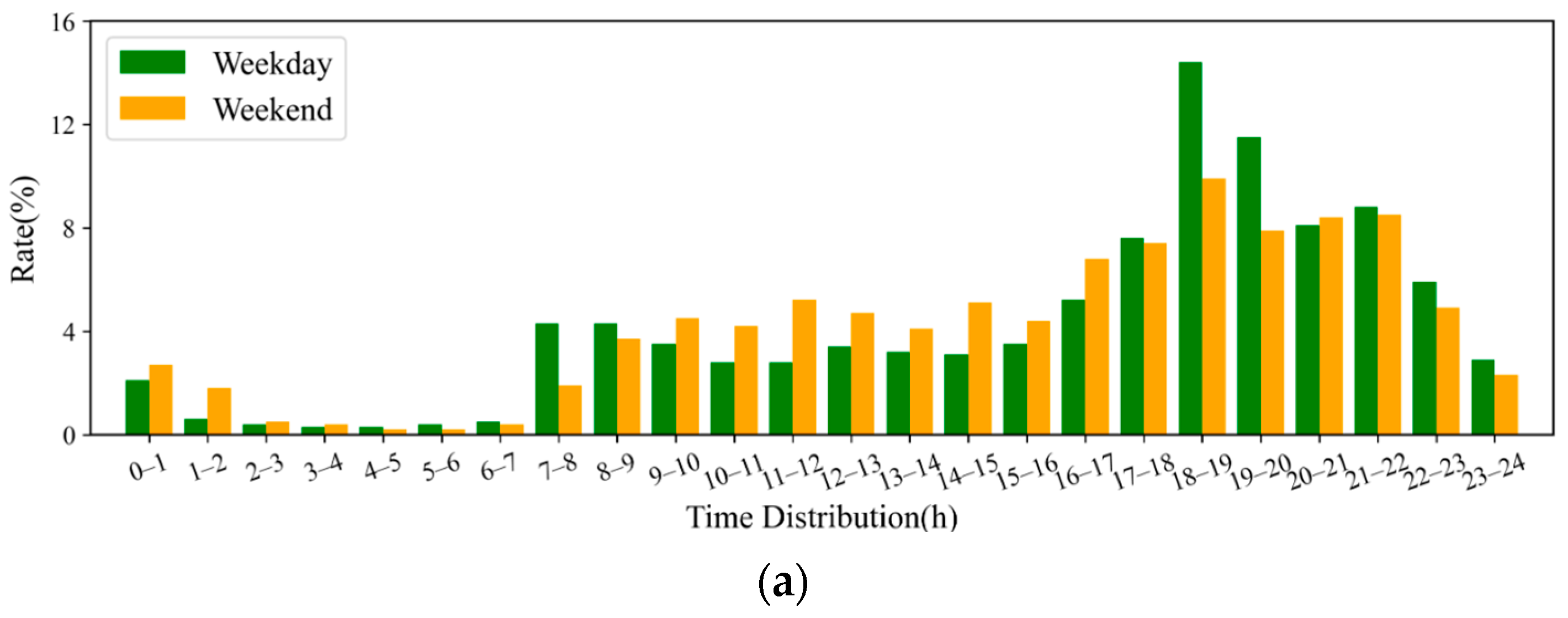
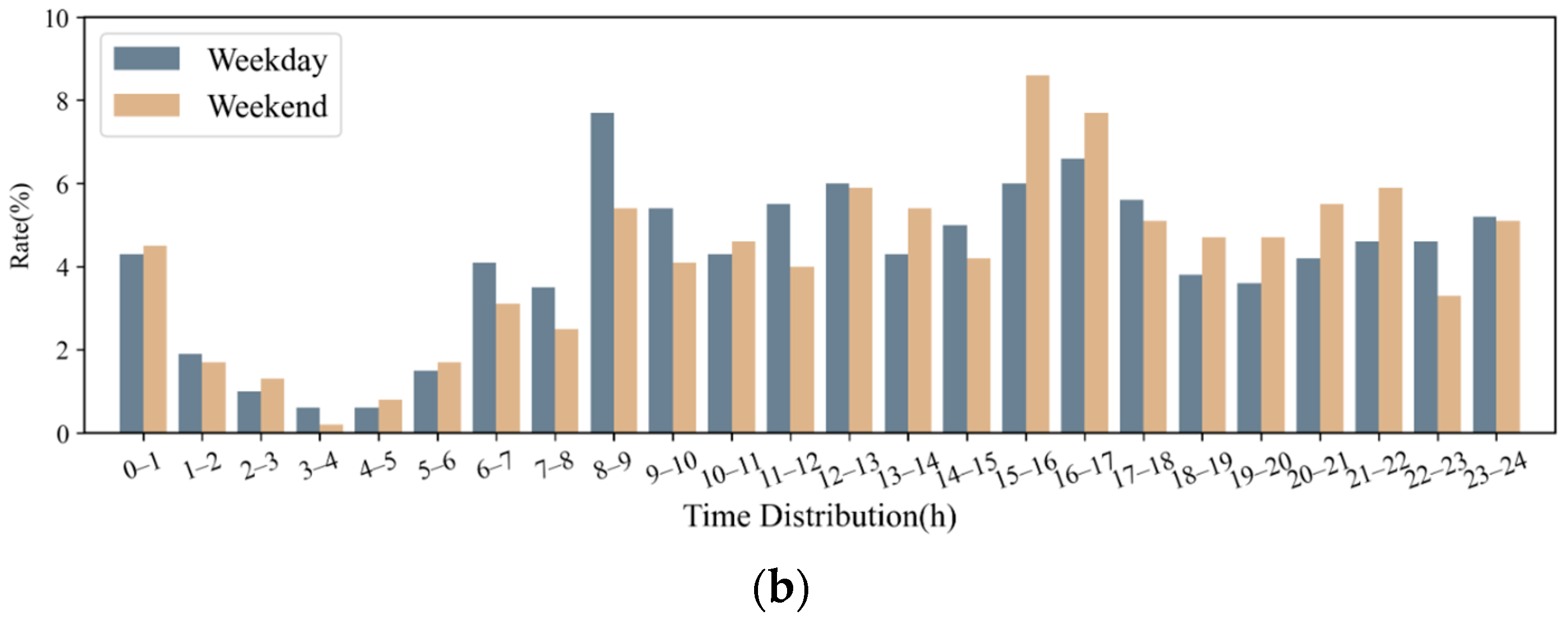
4.2.1. Charging Start Time
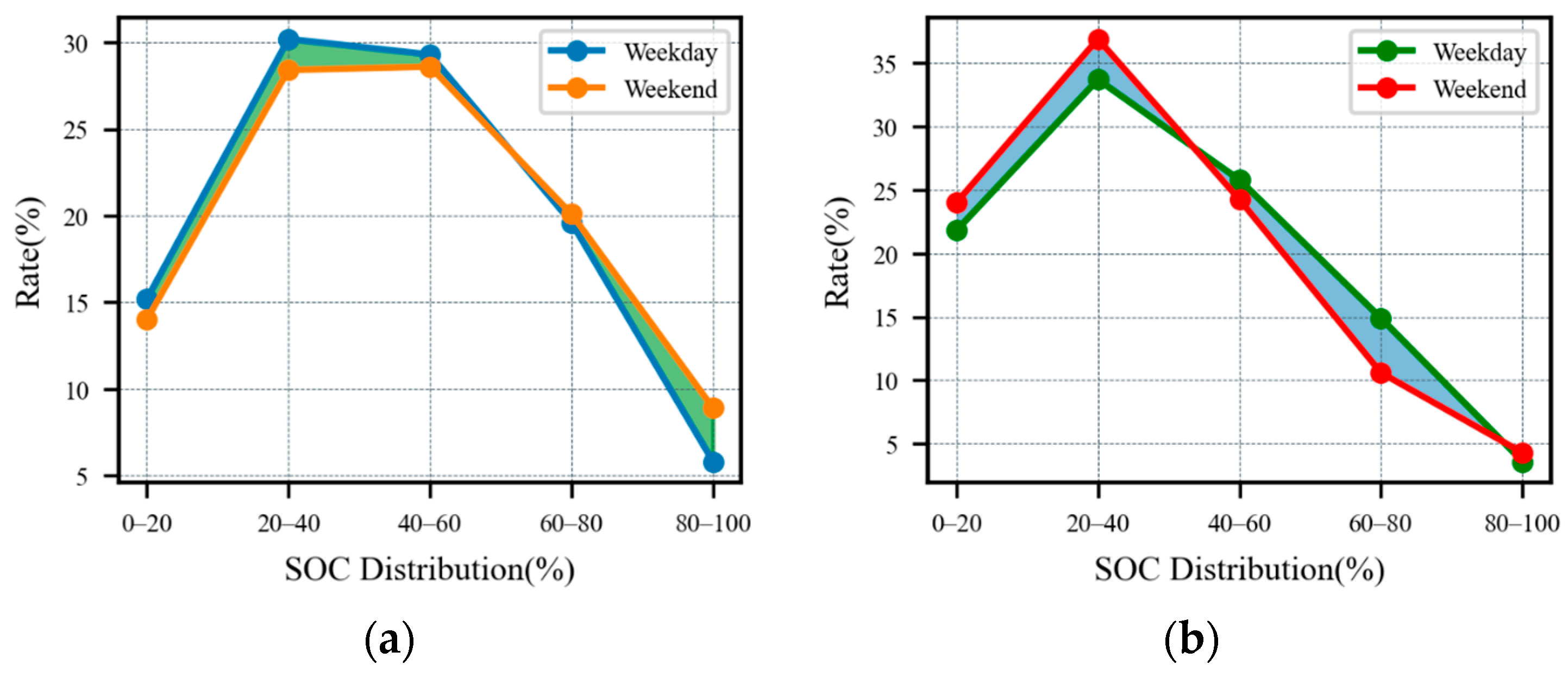
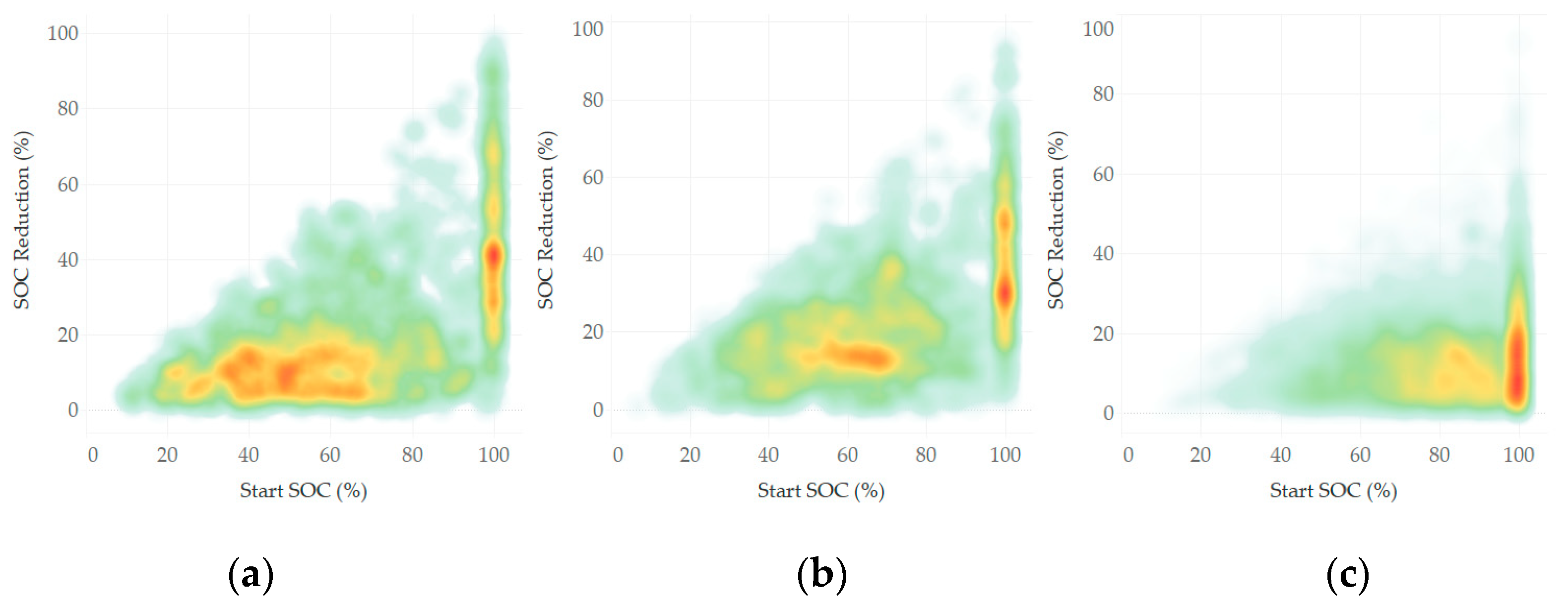
4.2.2. Charging Start SOC
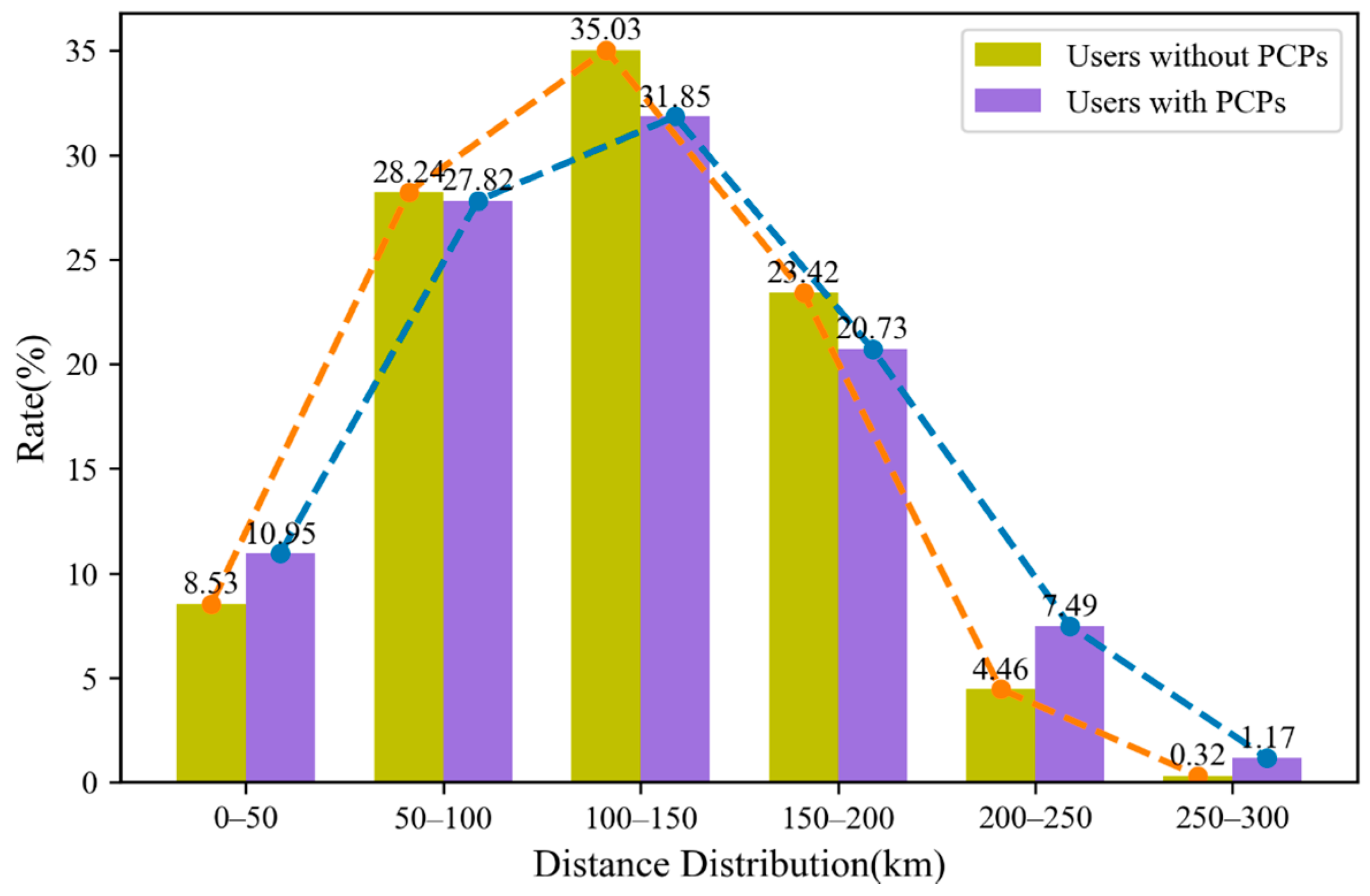
4.2.3. Driving Distance since Last Charge
4.2.4. Time since Last Charge
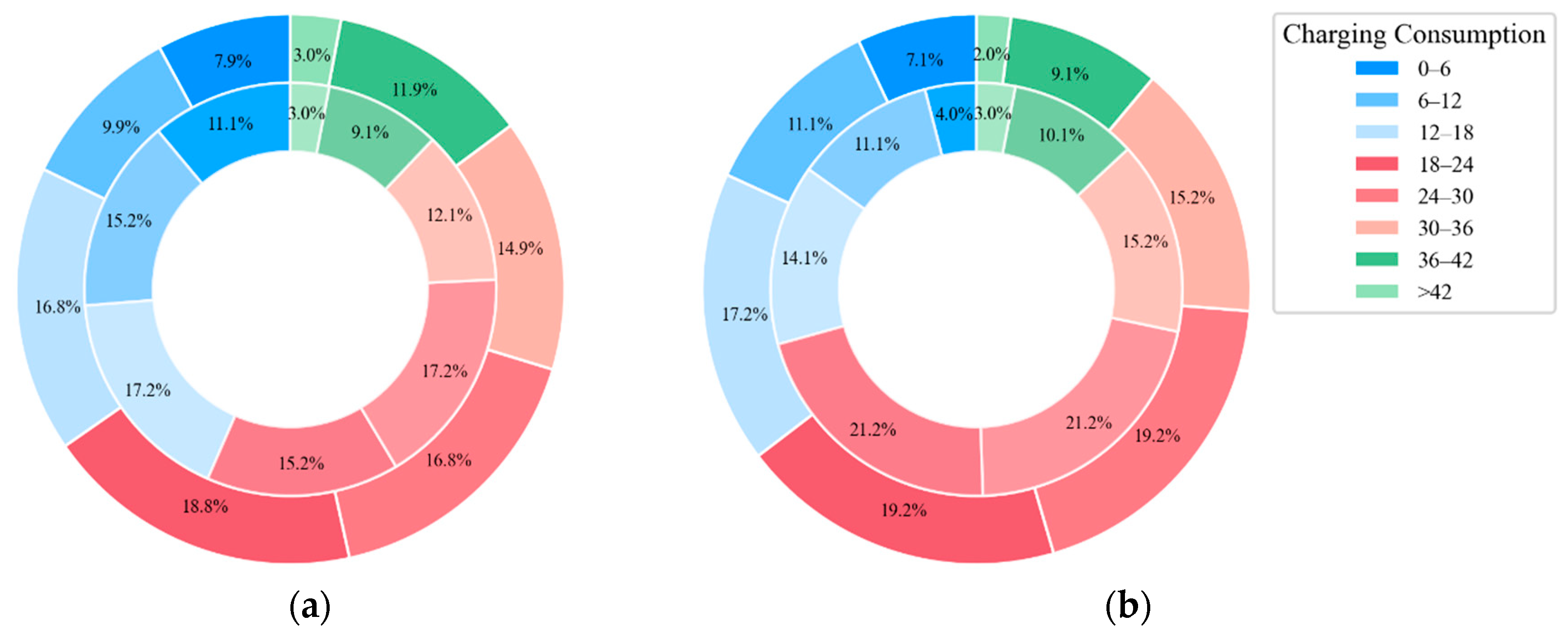
4.3. Charging Energy Consumption
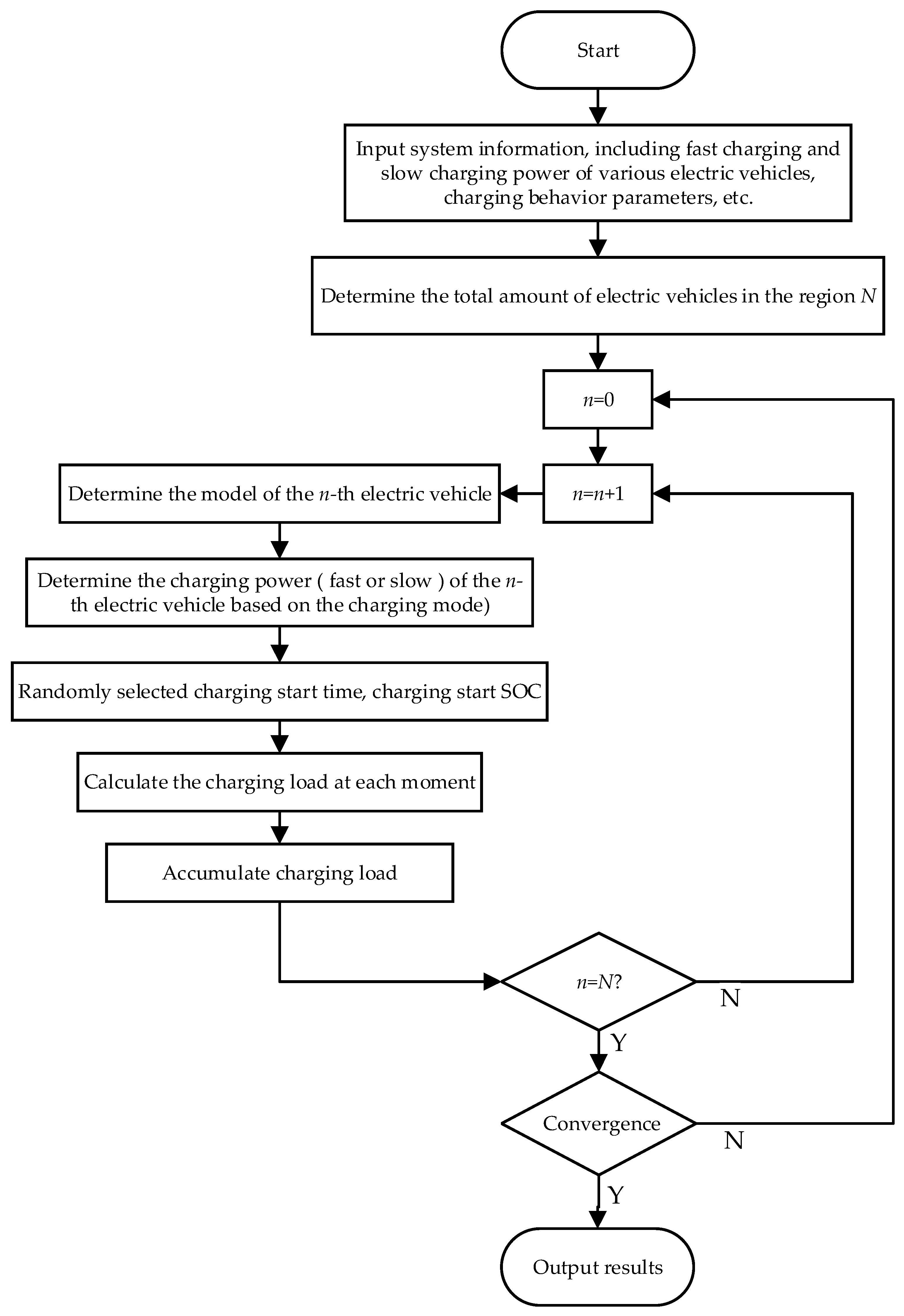
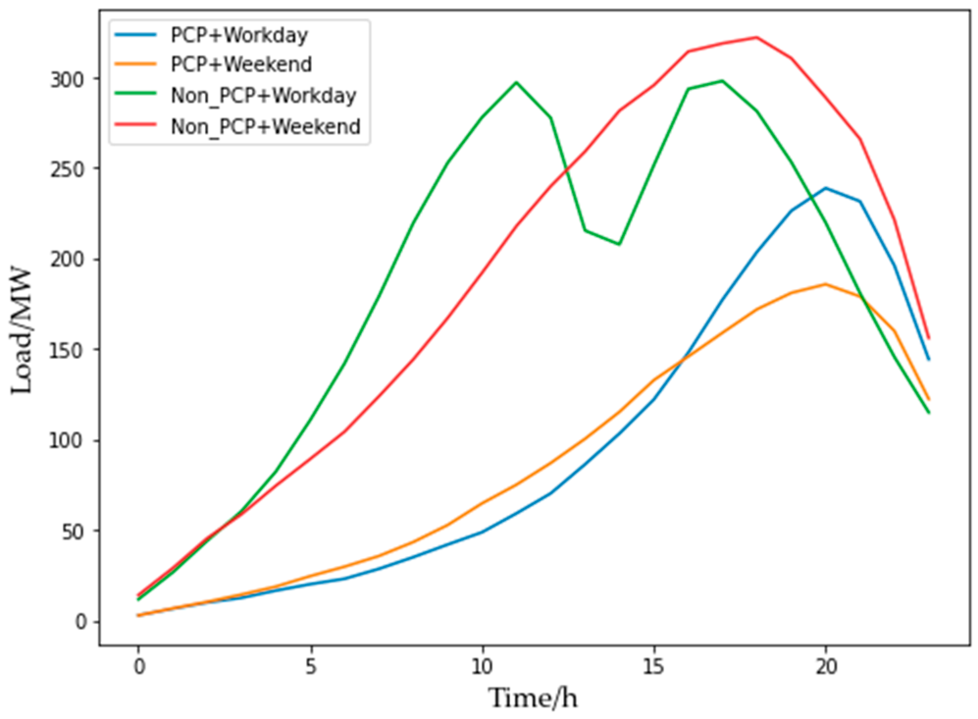
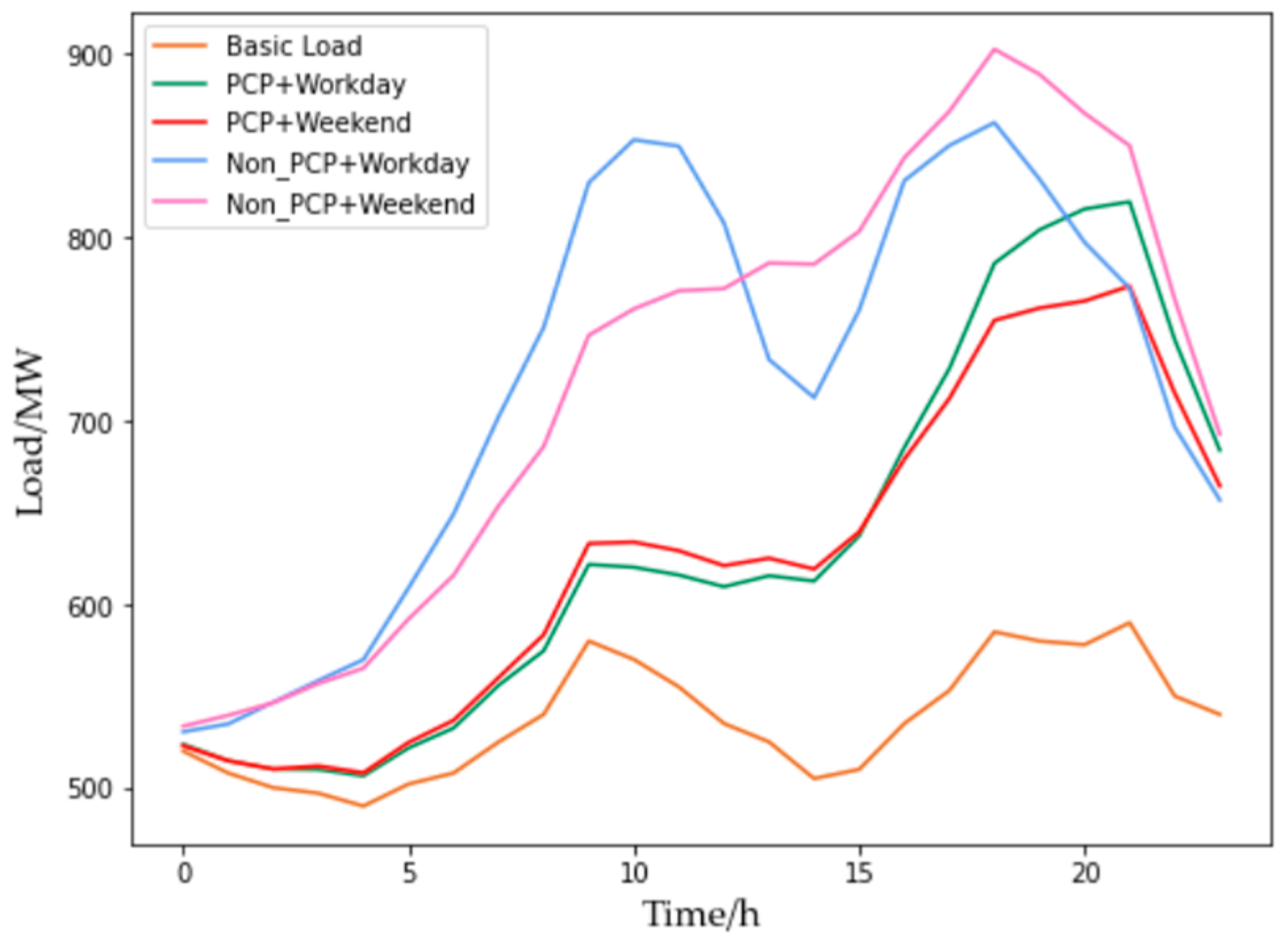
4.4. Prediction of Charging Load
- (1).
- Determine the total number N of BEVs in the region; this paper set N to 50,000.
- (2).
- Determine the model of BEV. Since the three types of vehicles in Table 2 occupy a large proportion of the BEV market, these three types of vehicles are taken as the main object. The possibilities of extracting these three types of vehicles are set to be the same.
- (3).
- Determine the charging mode of the electric vehicle, namely fast charging or slow charging.
- (4).
- According to the previous analysis results, the charging start time and the charging start SOC are randomly selected. The charging duration T(h) is calculated according to Equation (3).
- (5).
- The charging load of each time period is calculated in hours. Then the charging load curve of one vehicle is generated.
- (6).
- Repeat the above process, accumulate the charging load curve generated each time, and finally obtain the charging load curve of all vehicles.
- (7).
- Variance coefficient is used to judge whether the algorithm converges in this paper:
5. Influence of Trip Chain
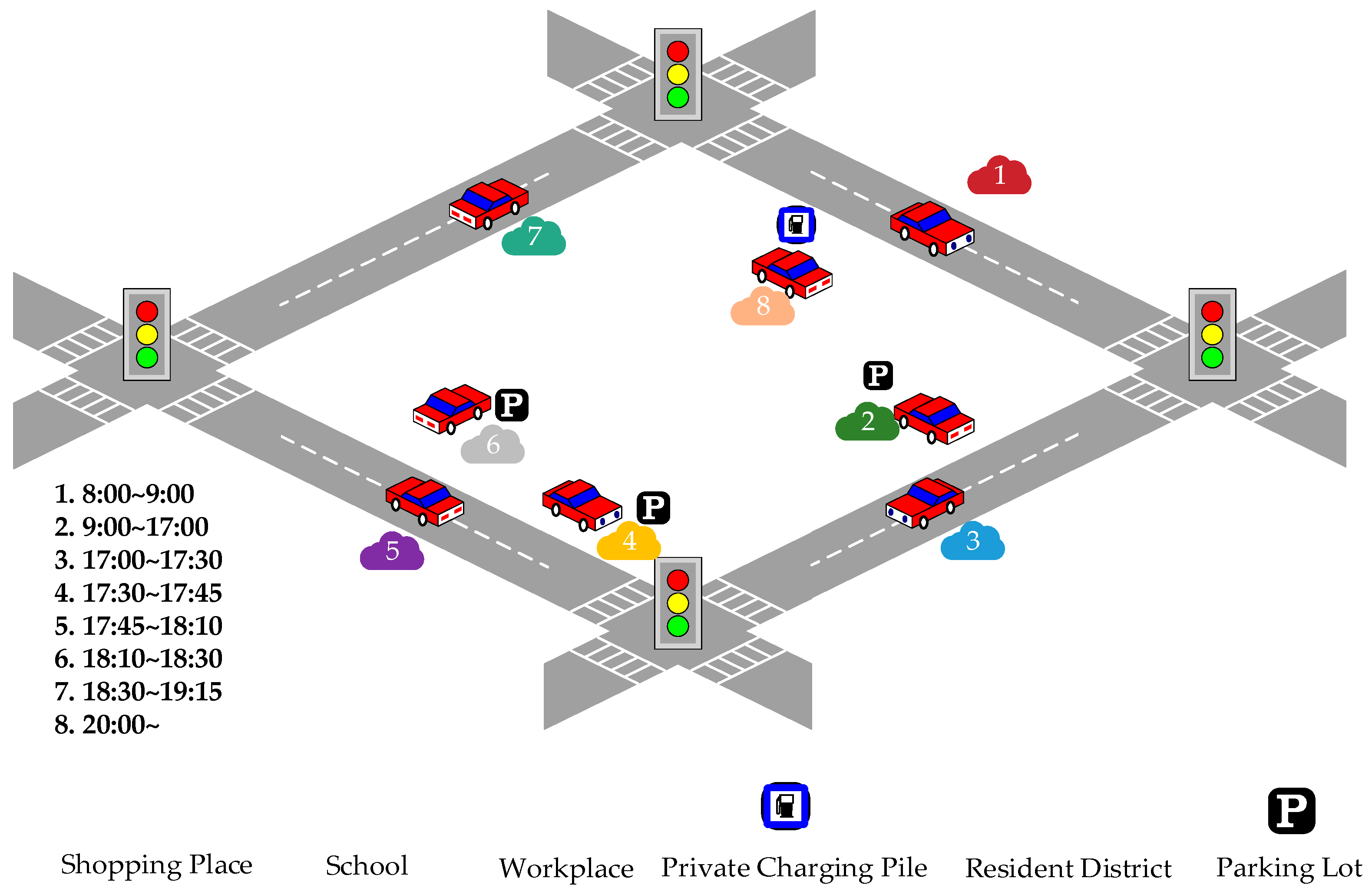
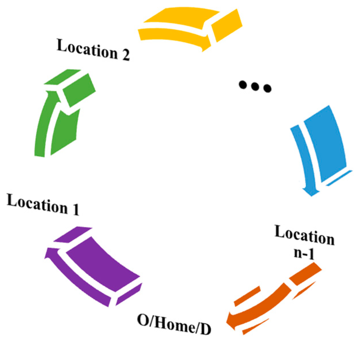
5.1. Trip Chain Generation
5.2. Key Factors Analysis
5.3. Influencing Analysis
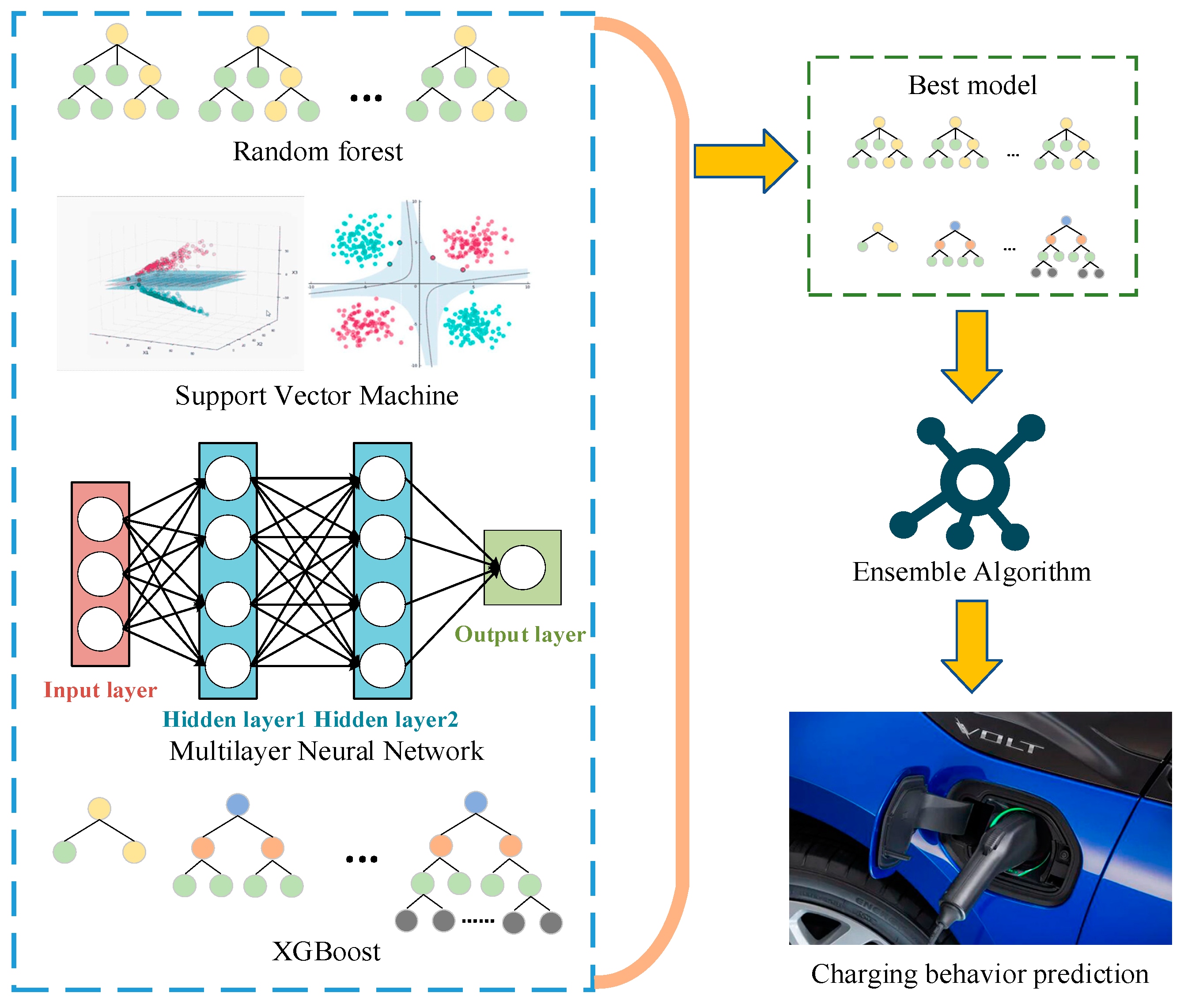
5.3.1. Support Vector Machine
5.3.2. XGBoost
5.3.3. Random Forest
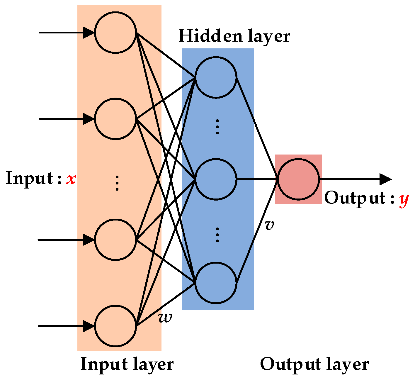
5.3.4. Deep Neural Network
6. Conclusions
Author Contributions
Funding
Data Availability Statement
Conflicts of Interest
Nomenclature
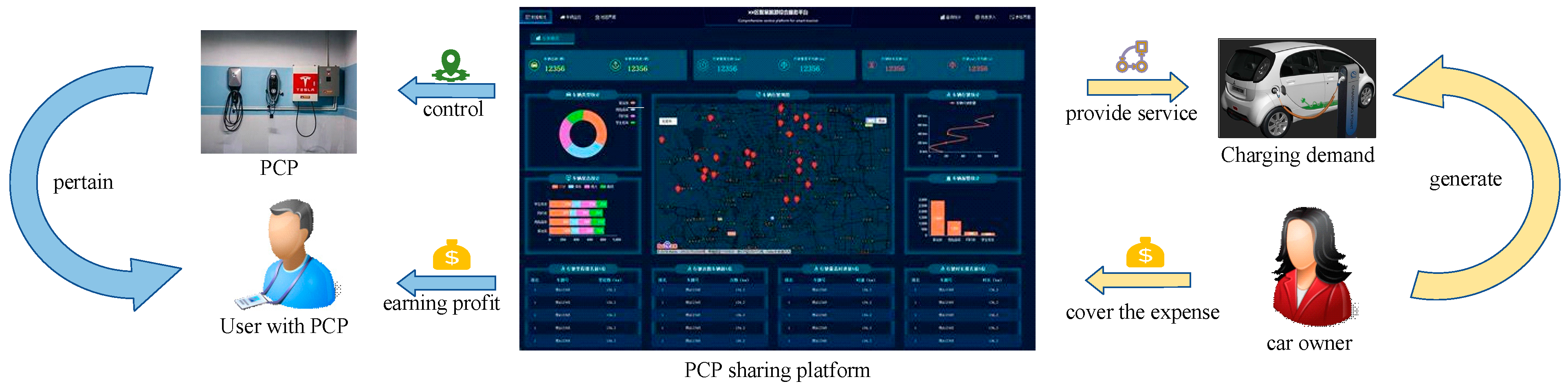
| PCP | Private charging pile |
| EV | Electric vehicle |
| BEV | Battery electric vehicle |
| MC | Monte Carlo |
| ABTCM | Agent-based trip chain model |
| MLR | Multinomial logistic regression |
| MLA | Machine learning algorithm |
| RF | Random forest |
| DNN | Deep neural network |
| SVM | Support vector machine |
| SOC | State of charge |
| POI | Point of interest |
| CART | Classification and regression tree |
References
- Hu, X.; Chen, N.; Wu, N.; Yin, B. The Potential Impacts of Electric Vehicles on Urban Air Quality in Shanghai City. Sustainability 2021, 13, 496. [Google Scholar] [CrossRef]
- Song, M.; Fisher, R.; Kwoh, Y. Technological Challenges of Green Innovation and Sustainable Resource Management with Large Scale Data. Technol. Forecast. Soc. Change 2019, 144, 361–368. [Google Scholar] [CrossRef]
- By the End of 2021, China’s New Energy Vehicle Ownership Reached 7.84 Million—Rolling News—Chinese Government Network. Available online: http://www.gov.cn/xinwen/2022-01/12/content_5667734.htm (accessed on 28 October 2022).
- Jian, L.; Yongqiang, Z.; Larsen, G.N.S.; Snartum, A. Implications of Road Transport Electrification: A Long-Term Scenario-Dependent Analysis in China. eTransportation 2020, 6, 100072. [Google Scholar] [CrossRef]
- China Charging Alliance: Number of Public Charging Piles Increased by 56.6% in September—China Electric Vehicle Association. Available online: http://www.ceva.org.cn/cn/viewnews/20221012/2022101210056.htm (accessed on 3 November 2022).
- Patt, A.; Aplyn, D.; Weyrich, P.; van Vliet, O. Availability of Private Charging Infrastructure Influences Readiness to Buy Electric Cars. Transp. Res. A Policy Pract. 2019, 125, 1–7. [Google Scholar] [CrossRef]
- Tan, Z.; Yang, Y.; Wang, P.; Li, Y. Charging Behavior Analysis of New Energy Vehicles. Sustainability 2021, 13, 4837. [Google Scholar] [CrossRef]
- Chen, Y.; Xia, D. Systematic Density Functional Theory Investigations on Cubic Lithium-Rich Iron-Based Li2FeO3: A Multiple Electrons Cationic and Anionic Redox Cathode Material. eTransportation 2021, 10, 100141. [Google Scholar] [CrossRef]
- Liu, T.; Yang, X.-G.; Ge, S.; Leng, Y.; Wang, C.-Y. Ultrafast Charging of Energy-Dense Lithium-Ion Batteries for Urban Air Mobility. eTransportation 2021, 7, 100103. [Google Scholar] [CrossRef]
- Hecht, C.; Victor, K.; Zurmühlen, S.; Sauer, D.U. Electric Vehicle Route Planning Using Real-World Charging Infrastructure in Germany. eTransportation 2021, 10, 100143. [Google Scholar] [CrossRef]
- Dixon, J.; Bell, K. Electric Vehicles: Battery Capacity, Charger Power, Access to Charging and the Impacts on Distribution Networks. eTransportation 2020, 4, 100059. [Google Scholar] [CrossRef]
- ‘14th Five-Year’ Beijing Electric Vehicle Charging Pile Will Reach 700,000—Local Government—Chinese Government Network. Available online: http://www.gov.cn/xinwen/2022-04/13/content_5684980.htm (accessed on 28 October 2022).
- Dominguez-Jimenez, J.A.; Campillo, J.E.; Montoya, O.D.; Delahoz, E.; Hernández, J.C. Seasonality Effect Analysis and Recognition of Charging Behaviors of Electric Vehicles: A Data Science Approach. Sustainability 2020, 12, 7769. [Google Scholar] [CrossRef]
- Xing, Q.; Chen, Z.; Zhang, Z.; Wang, R.; Zhang, T. Modelling Driving and Charging Behaviours of Electric Vehicles Using a Data-Driven Approach Combined with Behavioural Economics Theory. J. Clean. Prod. 2021, 324, 129243. [Google Scholar] [CrossRef]
- Nicholas, M.A.; Tal, G.; Davies, J.; Woodjack, J. DC Fast as the Only Public Charging Option? Scenario Testing from GPS-Tracked Vehicles. In Proceedings of the Transportation Research Board Conference, Washington, DC, USA, 22–26 January 2012; Available online: https://trid.trb.org/view/1130070 (accessed on 29 November 2022).
- He, Y.; Kockelman, K.M.; Perrine, K.A. Optimal Locations of U.S. Fast Charging Stations for Long-Distance Trip Completion by Battery Electric Vehicles. J. Clean. Prod. 2019, 214, 452–461. [Google Scholar] [CrossRef]
- Xu, Z.; Wang, J.; Lund, P.D.; Zhang, Y. Estimation and Prediction of State of Health of Electric Vehicle Batteries Using Discrete Incremental Capacity Analysis Based on Real Driving Data. Energy 2021, 225, 120160. [Google Scholar] [CrossRef]
- GaryLea ChangeCoordinate 2022. Available online: https://github.com/GaryLea/ChangeCoordinate (accessed on 21 November 2022).
- Geo/Inverse Geocoding—API Documentation—Development Guide—Web Services API—Amap API. Available online: https://developer.amap.com/api/webservice/guide/api/georegeo (accessed on 4 November 2022).
- Electric Pile Home—Electric Life. Available online: https://www.powerlife.com.cn/pile/ops/map/default.html (accessed on 22 November 2022).
- Jordán, J.; Palanca, J.; Del Val, E.; Julian, V.; Botti, V. A Multi-Agent System for the Dynamic Emplacement of Electric Vehicle Charging Stations. Appl. Sci. 2018, 8, 313. [Google Scholar] [CrossRef] [Green Version]
- Pagany, R.; Marquardt, A.; Zink, R. Electric Charging Demand Location Model—A User- and Destination-Based Locating Approach for Electric Vehicle Charging Stations. Sustainability 2019, 11, 2301. [Google Scholar] [CrossRef] [Green Version]
- Lu, Z.; Zhang, Q.; Yuan, Y.; Tong, W. Optimal Driving Range for Battery Electric Vehicles Based on Modeling Users’ Driving and Charging Behavior. J. Adv. Transp. 2020, 2020, 8813137. [Google Scholar] [CrossRef]
- Quirós-Tortós, J.; Ochoa, L.F.; Lees, B. A Statistical Analysis of EV Charging Behavior in the UK. In Proceedings of the IEEE/PES Innovative Smart Grid Technologies ISGT Latin America, Montevideo, Uruguay, 5–7 October 2015; pp. 445–449. [Google Scholar]
- Canizes, B.; Soares, J.; Vale, Z.; Corchado, J.M. Optimal Distribution Grid Operation Using DLMP-Based Pricing for Electric Vehicle Charging Infrastructure in a Smart City. Energies 2019, 12, 686. [Google Scholar] [CrossRef] [Green Version]
- Xu, M.; Yang, H.; Wang, S. Mitigate the Range Anxiety: Siting Battery Charging Stations for Electric Vehicle Drivers. Transp. Res. C Emerg. Technol. 2020, 114, 164–188. [Google Scholar] [CrossRef]
- Yang, Y.; Yao, E.; Yang, Z.; Zhang, R. Modeling the Charging and Route Choice Behavior of BEV Drivers. Transp. Res. C Emerg. Technol. 2016, 65, 190–204. [Google Scholar] [CrossRef]
- Williard, N.; He, W.; Osterman, M.; Pecht, M. Comparative Analysis of Features for Determining State of Health in Lithium-Ion Batteries. IJPHM 2020, 4, 1–7. [Google Scholar] [CrossRef]
- Wan, X.; Wang, W.; Liu, J.; Tong, T. Estimating the Sample Mean and Standard Deviation from the Sample Size, Median, Range and/or Interquartile Range. BMC Med. Res. Methodol. 2014, 14, 135. [Google Scholar] [CrossRef] [PubMed] [Green Version]
- Weldon, P.; Morrissey, P.; Brady, J.; O’Mahony, M. An Investigation into Usage Patterns of Electric Vehicles in Ireland. Transp. Res. D Transp. Environ. 2016, 43, 207–225. [Google Scholar] [CrossRef]
- Sun, D.; Ou, Q.; Yao, X.; Gao, S.; Wang, Z.; Ma, W.; Li, W. Integrated Human-Machine Intelligence for EV Charging Prediction in 5G Smart Grid. EURASIP J. Wirel. Commun. Netw. 2020, 2020, 139. [Google Scholar] [CrossRef]
- Gonzalez Venegas, F.; Petit, M.; Perez, Y. Plug-in Behavior of Electric Vehicles Users: Insights from a Large-Scale Trial and Impacts for Grid Integration Studies. eTransportation 2021, 10, 100131. [Google Scholar] [CrossRef]
- Siddique, C.; Afifah, F.; Guo, Z.; Zhou, Y. Data Mining of Plug-in Electric Vehicles Charging Behavior Using Supply-Side Data. Energy Policy 2022, 161, 112710. [Google Scholar] [CrossRef]
- Ren, Y.; Lan, Z.; Yu, H.; Jiao, G. Analysis and Prediction of Charging Behaviors for Private Battery Electric Vehicles with Regular Commuting: A Case Study in Beijing. Energy 2022, 253, 124160. [Google Scholar] [CrossRef]
- Zhao, P.; Guan, H.; Wei, H.; Liu, S. Mathematical Modeling and Heuristic Approaches to Optimize Shared Parking Resources: A Case Study of Beijing, China. Transp. Res. Interdiscip. Perspect. 2021, 9, 100317. [Google Scholar] [CrossRef]
- Lin, H.; Fu, K.; Wang, Y.; Sun, Q.; Li, H.; Hu, Y.; Sun, B.; Wennersten, R. Characteristics of Electric Vehicle Charging Demand at Multiple Types of Location—Application of an Agent-Based Trip Chain Model. Energy 2019, 188, 116122. [Google Scholar] [CrossRef]
- Almaghrebi, A.; Aljuheshi, F.; Rafaie, M.; James, K.; Alahmad, M. Data-Driven Charging Demand Prediction at Public Charging Stations Using Supervised Machine Learning Regression Methods. Energies 2020, 13, 4231. [Google Scholar] [CrossRef]
- Frendo, O.; Gaertner, N.; Stuckenschmidt, H. Improving Smart Charging Prioritization by Predicting Electric Vehicle Departure Time. IEEE Trans. Intell. Transp. Syst. 2021, 22, 6646–6653. [Google Scholar] [CrossRef]
- Chung, Y.-W.; Khaki, B.; Li, T.; Chu, C.; Gadh, R. Ensemble Machine Learning-Based Algorithm for Electric Vehicle User Behavior Prediction. Appl. Energy 2019, 254, 113732. [Google Scholar] [CrossRef]
- Ge, X.; Shi, L.; Fu, Y.; Muyeen, S.M.; Zhang, Z.; He, H. Data-Driven Spatial-Temporal Prediction of Electric Vehicle Load Profile Considering Charging Behavior. Electr. Power Syst. Res. 2020, 187, 106469. [Google Scholar] [CrossRef]
- Shahriar, S.; Al-Ali, A.R.; Osman, A.H.; Dhou, S.; Nijim, M. Prediction of EV Charging Behavior Using Machine Learning. IEEE Access 2021, 9, 111576–111586. [Google Scholar] [CrossRef]
- Khwaja, A.S.; Venkatesh, B.; Anpalagan, A. Short-Term Individual Electric Vehicle Charging Behavior Prediction Using Long Short-Term Memory Networks. In Proceedings of the 2020 IEEE 25th International Workshop on Computer Aided Modeling and Design of Communication Links and Networks (CAMAD), Pisa, Italy, 14–16 September 2020; pp. 1–7. [Google Scholar]
- Li, Z.; Feng, X.; Wu, Z.; Yang, C.; Bai, B.; Yang, Q. Classification of Atrial Fibrillation Recurrence Based on a Convolution Neural Network With SVM Architecture. IEEE Access 2019, 7, 77849–77856. [Google Scholar] [CrossRef]
- Naimi, A.I.; Balzer, L.B. Stacked Generalization: An Introduction to Super Learning. Eur. J. Epidemiol. 2018, 33, 459–464. [Google Scholar] [CrossRef] [PubMed]


| Time | Vehicle ID | Vehicle State | Charging State | Speed (km/h) | Mileage (km) | Longitude | Latitude | SOC (%) |
|---|---|---|---|---|---|---|---|---|
| 1 January 2020 00:00:06 | 98,341 | 2 | 1 | 0 | 34,279 | 116.3608 | 40.1142 | 68 |
| 1 January 2020 00:00:16 | 98,341 | 2 | 1 | 0 | 34,279 | 116.3608 | 40.1142 | 68 |
| … | ||||||||
| 4 August 2020 07:12:47 | 98,341 | 1 | 3 | 21.8 | 41,911 | 116.2863 | 40.0129 | 43 |
| 4 August 2020 07:12:57 | 98,341 | 1 | 2 | 18.3 | 41,911 | 116.2857 | 40.0128 | 43 |
| … | ||||||||
| 4 November 2020 02:17:28 | 98,341 | 2 | 1 | 0 | 45,970 | 116.3608 | 40.1142 | 100 |
| Brand | GAC Thriving 14 | BAIC EU260 | SAIC Roewe ERX5 |
|---|---|---|---|
 |  |  | |
| Capacity (kWh) | 47.5 | 37.8 | 48.3 |
| Battery Type | Lithium iron phosphate battery | Nickel–Cobalt–Manganese | Nickel–Cobalt–Manganese |
| Fast Charge Power (kW) | 49.15 | 50.87 | 63.32 |
| Slow Charge Power(kW) | 3.05 | 6.13 | 6.42 |
| Driving Range (km) | 253 | 260 | 320 |
| Maximum Speed (km/h) | 150 | 140 | 135 |
| Vehicle State | Charging State | Speed | State | |||
|---|---|---|---|---|---|---|
| 1 | + | 3 | + | 0 | Status 1. Parking but power on | |
| 1 | + | 3 | + | Status 2. Driving | ||
| 2 | + | 3 | + | 0 | Status 3. Parking and power off | |
| 2 | + | 1 | + | 0 | Status 4. Parking and charging | |
| 2 | + | 4 | + | 0 | Status 5. Charging completed but not unplugged |
| Vehicle ID | Name | District | Minimum Range (m) | Type | Position |
|---|---|---|---|---|---|
| 98,363 | Beijing University of Chinese Medicine | Chaoyang District | 145.2680 | School | 116.428250, 39.971307 |
| Decimal | 0 | 1 | 2 | 3 | 4 | 5 | 6 | 7 | 8 | 9 | 10 | 11 | 12 | 13 | 14 | 15 | 16 | 17 | 18 | 19 | 20 | 21 | 22 | 23 | 24 | 25 | 26 | 27 | 28 | 29 | 30 | 31 |
|---|---|---|---|---|---|---|---|---|---|---|---|---|---|---|---|---|---|---|---|---|---|---|---|---|---|---|---|---|---|---|---|---|
| Base32 | 0 | 1 | 2 | 3 | 4 | 5 | 6 | 7 | 8 | 9 | b | c | d | e | f | g | h | j | k | m | n | p | q | r | s | t | u | v | w | x | y | z |
| Minimum | Q1 | Median | Q3 | Maximum | ||
|---|---|---|---|---|---|---|
| Have PCP? | Yes | 1.0 | 79.00 | 117.00 | 159.00 | 288.00 |
| No | 1.0 | 83.00 | 120.00 | 154.25 | 296.00 |
| Minimum | Q1 | Median | Q3 | Maximum | ||
|---|---|---|---|---|---|---|
| Have PCP? | Yes | 0.27 | 20.74 | 51.44 | 109.66 | 2592.27 |
| No | 0.26 | 7.58 | 17.25 | 48.61 | 3145.59 |
| Minimum | Q1 | Median | Q3 | Maximum | |||
|---|---|---|---|---|---|---|---|
| Have PCP? | Yes | Total | 0.47 | 14.08 | 22.33 | 31.40 | 47.82 |
| Weekday | 0.47 | 14.73 | 22.80 | 31.86 | 47.82 | ||
| Weekend | 0.48 | 11.59 | 20.90 | 29.95 | 47.03 | ||
| No | Total | 0.41 | 14.49 | 22.36 | 30.64 | 46.08 | |
| Weekday | 0.41 | 14.25 | 22.33 | 30.43 | 46.08 | ||
| Weekend | 0.83 | 16.56 | 23.44 | 31.45 | 45.60 |
| Type | Non-PCP Charging | PCP Charging | No-Charging | Total |
|---|---|---|---|---|
| Number of chains | 1547 | 2365 | 9429 | 13,341 |
| Rate (%) | 11.59 | 17.73 | 70.68 | 100 |
| Type | Variables | Description |
|---|---|---|
| Vehicle State | Start SOC | SOC at the beginning of the journey |
| SOC decline | SOC declined in the trip | |
| Start Time | The start time of the trip | |
| Travel time | Travel time (excluding parking) | |
| Mileage | Distance in trip | |
| Average Speed | Average speed in a trip | |
| External environment | Average Temperature | Temperature of the day of travel |
| Month | Represents the change of seasons | |
| Week | Whether or not is weekday |
| Variables | Coefficient | Standard Error | Odds Ratio | p | [95% Conf. Interval] | |
|---|---|---|---|---|---|---|
| PCP charging | ||||||
| Start SOC (%) | −4.513 | 0.161 | 0.011 | <0.001 | 0.009 | 0.014 |
| SOC Decline (%) | 3.574 | 0.129 | 35.651 | <0.001 | 15.940 | 79.738 |
| Mileage (km) | 4.134 | 0.411 | 62.413 | <0.001 | 21.387 | 182.135 |
| Average Speed (km/h) | 1.294 | 0.546 | 3.649 | <0.001 | 2.269 | 5.867 |
| Week | 0.023 | 0.242 | 1.023 | 0.777 | 0.872 | 1.200 |
| Start Time (h) | −1.435 | 0.081 | 0.238 | <0.001 | 0.151 | 0.374 |
| Travel Time (h) | −0.190 | 0.231 | 0.827 | 0.202 | 0.617 | 1.107 |
| Month | −0.026 | 0.149 | 0.974 | 0.820 | 0.777 | 1.221 |
| Average Temperature ( | −0.661 | 0.115 | 0.516 | <0.001 | 0.401 | 0.665 |
| Non-PCP charging | ||||||
| Start SOC (%) | −4.897 | 0.151 | 0.007 | <0.001 | 0.006 | 0.010 |
| SOC Decline (%) | 5.360 | 0.497 | 212.682 | <0.001 | 80.303 | 563.285 |
| Mileage (km) | −0.135 | 0.686 | 0.873 | 0.843 | 0.228 | 3.351 |
| Average Speed (km/h) | 3.588 | 0.273 | 36.157 | <0.001 | 21.159 | 61.789 |
| Week | −0.020 | 0.096 | 0.980 | 0.833 | 0.812 | 1.182 |
| Start Time (h) | −2.535 | 0.279 | 0.079 | <0.001 | 0.046 | 0.137 |
| Travel Time (h) | −1.086 | 0.186 | 0.338 | <0.001 | 0.235 | 0.486 |
| Month | 0.411 | 0.133 | 1.509 | 0.002 | 1.163 | 1.957 |
| Average Temperature ( | −0.682 | 0.149 | 0.506 | <0.001 | 0.377 | 0.678 |
| Type | Precision | Recall | F1-score | ||||||
|---|---|---|---|---|---|---|---|---|---|
| PCPC | NPCPC | NC | PCPC | NPCPC | NC | PCPC | NPCPC | NC | |
| ANN | 0.67 | 0.68 | 0.77 | 0.68 | 0.76 | 0.68 | 0.67 | 0.71 | 0.72 |
| RF | 0.84 | 0.88 | 0.85 | 0.87 | 0.91 | 0.79 | 0.86 | 0.90 | 0.82 |
| XGBoost | 0.84 | 0.89 | 0.87 | 0.89 | 0.91 | 0.81 | 0.87 | 0.90 | 0.84 |
| SVM | 0.54 | 0.56 | 0.78 | 0.29 | 0.13 | 0.96 | 0.38 | 0.21 | 0.86 |
| Stacking Ensemble | 0.86 | 0.86 | 0.91 | 0.89 | 0.90 | 0.83 | 0.87 | 0.90 | 0.85 |
| Voting Ensemble | 0.85 | 0.90 | 0.87 | 0.89 | 0.91 | 0.81 | 0.87 | 0.90 | 0.84 |
Disclaimer/Publisher’s Note: The statements, opinions and data contained in all publications are solely those of the individual author(s) and contributor(s) and not of MDPI and/or the editor(s). MDPI and/or the editor(s) disclaim responsibility for any injury to people or property resulting from any ideas, methods, instructions or products referred to in the content. |
© 2023 by the authors. Licensee MDPI, Basel, Switzerland. This article is an open access article distributed under the terms and conditions of the Creative Commons Attribution (CC BY) license (https://creativecommons.org/licenses/by/4.0/).
Share and Cite
Tian, H.; Sun, Y.; Hu, F.; Du, J. Charging Behavior Analysis Based on Operation Data of Private BEV Customers in Beijing. Electronics 2023, 12, 373. https://doi.org/10.3390/electronics12020373
Tian H, Sun Y, Hu F, Du J. Charging Behavior Analysis Based on Operation Data of Private BEV Customers in Beijing. Electronics. 2023; 12(2):373. https://doi.org/10.3390/electronics12020373
Chicago/Turabian StyleTian, Hao, Yujuan Sun, Fangfang Hu, and Jiuyu Du. 2023. "Charging Behavior Analysis Based on Operation Data of Private BEV Customers in Beijing" Electronics 12, no. 2: 373. https://doi.org/10.3390/electronics12020373