Article

Dual-Arm Cluster Tool Scheduling for Reentrant Wafer Flows

1
Institute of Systems Engineering and Collaborative Laboratory for Intelligent Science and Systems, Macau University of Science and Technology, Macao 999078, China
2
State Key Laboratory of Precision Electronic Manufacturing Technology and Equipment, Guangdong University of Technology, Guangzhou 510006, China
3
IKAS Industries Technology (Suzhou) Company Ltd., Suzhou 215000, China
*
Author to whom correspondence should be addressed.
Electronics 2023, 12(11), 2411; https://doi.org/10.3390/electronics12112411
Submission received: 16 April 2023 / Revised: 22 May 2023 / Accepted: 22 May 2023 / Published: 26 May 2023
(This article belongs to the Topic Advanced Systems Engineering: Theory and Applications)

Abstract

:
Cluster tools are the key equipment in semiconductor manufacturing systems. They have been widely adopted for many wafer fabrication processes, such as chemical and physical vapor deposition processes. Reentrant wafer flows are commonly seen in cluster tool operations for deposition processes. It is very complicated to schedule cluster tools with reentrant processes. For a dual-arm cluster tool with two-time reentering, the existing studies point out that a one-wafer periodical (1-WP) schedule can be found, and it is optimal in terms of productivity. However, for some wafer fabrication processes, wafers should be processed at some PMs more than two times. This gives rise to a question of whether there still exists a 1-WP schedule for dual-arm cluster tools with the number of reentering times being more than two such that the cycle time of a tool can reach the lower bound. This problem is still open, and this is what this work wants to tackle. For a dual-arm cluster tool with the number of reentering times being k (>2) times, if there does not exist a value f ∈ {1, 2 …} such that k = 3f, theoretical proofs are given to show that a 1-WP schedule can be found, otherwise it does not exist. For cases with a 1-WP schedule, the cycle time can be obtained by analytical expressions. For the cases without a 1-WP schedule, two new methods for a three-wafer periodical schedule are proposed to improve the system productivity by comparing it with an existing three-wafer periodical schedule. The applications of the obtained results are demonstrated by examples. Wafer residency time constraints are required for some wafer fabrication processes. Note that the results obtained in this work cannot be directly applied to cluster tools with both reentrant wafer flows and wafer residency time constraints. Nevertheless, schedulablity and scheduling analyses for that applications can be conducted based on the obtained results in this work.

1. Introduction

In semiconductor manufacturing, cluster tools have been widely adopted for wafer fabrication. Such a tool compactly integrates several process modules (PMs), a robot, and two loadlocks (LLs). Moreover, it adopts a single-wafer processing technology such that wafers are processed one by one in a PM. With a single- or dual-arm robot, a tool is called a single-arm cluster tool (SACT) or dual-arm cluster tool (DACT), as shown in Figure 1a,b.
In an SACT or a DACT as shown in Figure 1, PMs are filled with chemicals for wafer processing, and the internal temperature in PMs is required to be high for some wafer fabrication processes. The robot in the center of a tool is used to transport wafers among the PMs. LLs have two doors. One faces the internal chamber in which there are several PMs, while the other faces outside. LLs are used to ensure the internal vacuum processing environment.
In semiconductor fabs, 25 wafers are grouped into a lot and held in a front opening unified pod (FOUP) [1]. FOUPs are transported to the right areas for wafer fabrication according to recipes. The recipes of wafers in a lot are identical. In a cluster tool, after a wafer lot is loaded into an LL, the LL is pumped into a vacuum environment. Then, the wafers can be delivered to PMs to be processed according to their recipes. After wafers in an LL are completed, then the raw wafers from the other LL are fed to PMs to be processed such that the tool can operate under a steady state without interruption [1,2].
For some wafer fabrication processes, wafers are required to visit some PMs for more than one time. Such a wafer fabrication process is called a reentering process. Atomic layer deposition (ALD) and plasma-enhanced chemical vapor deposition (PECVD) are such typical processes. For the ALD process, deposition processes should be repeatedly performed several times, even more than five. The first deposition layer requires three process steps: Al2O3 deposition, Ta2O5 deposition, and oxidation process. Each subsequent deposition layer repeats the last two process steps [3]. For a PECVD process, PECVD tools are used for depositing thin films onto silicon wafer substrates, which is one of the crucial steps in the manufacturing of microelectronic circuits and solar cells [4]. For reentering processes, the reentering operations should be performed under identical processing conditions. This presents a requirement that only one PM is configured to serve a processing step.
For a DACT with reentrant wafer flows, Qiao et al. [5] developed a one-wafer periodical (1-WP) scheduling method by adjusting the processing progresses of wafers at different steps such that a 1-WP schedule can be obtained. Moreover, theoretical proofs for its optimality are provided in [5]. However, the study is done for a 2-time reentering process, and it is not known if it is applicable to processes with the reentering times being more than two. In practice, for some reentering processes, wafers are required to visit some PMs for k (≥2) times. Recently, it has been found that a 1-WP schedule cannot be obtained for a DACT with k-time reentrant processes if there exists a value f ∈ ℕ = {1, 2 …} such that k = 3f holds. This implies that the method in [5] is not applicable to such cases, which motivates us to do this work. Further, this work aims at solving the scheduling problem of DACTs with k-time (k ≥ 3) reentrant processes such that the solutions to DACTs with reentrant processes are complete.

2. Literature Review

In SACTs and DACTs, the time taken for robot tasks, including placing, picking, and moving, is actually quite short in comparison with wafer processing time in PMs. Thus, for SACTs, a backward strategy is optimal in terms of productivity [6,7], while for DACTs, a swap strategy is optimal [8]. Further, studies on modeling and scheduling SACTs and DACTs were conducted in [8,9,10]. With two wafer types and one shared PM, the scheduling analysis was done for DACTs in [11]. The results obtained in the above-mentioned studies are based on the assumption that there are no wafer residency time constraints (WRTCs).
For some wafer fabrication processes, WRTCs are imposed, which requires that after a wafer is processed in a PM, it should be removed from the PM within a limited time interval, otherwise it would be damaged by the high temperature and chemical gas in the PM. In [12,13], methods were proposed to find optimal periodical schedules for DACTs with WRTCs. Further, based on Petri nets, a mixed integer programming (MIP) method was presented in [14] to get optimal cyclic schedules for both SACTs and DACTs with various wafer processing flows. To improve the computational efficiency in finding an optimal solution for SACTs and DACTs with WRTCs, schedulability conditions under which a feasible schedule exists were established in [15,16]. If schedulable checked by such conditions, the authors established analytical expressions to find optimal solutions. With multiple wafer types, wafer delay analysis and workload balancing of parallel PMs were conducted in [17]. Moreover, PM configuring problem of residency time-constrained DACTs was investigated, and a polynomial-complexity algorithm was developed to find optimal cyclic schedules in [18].
In practice, the time required for robot activities and wafer processing might be disturbed. Such a time variation may result in a feasible schedule obtained under the deterministic activity time assumption becoming infeasible. Thus, a robust scheduling method is necessary for cluster tools with activity time variation. To do so, in [19], based on Petri nets, a real-time control policy was proposed for DACTs with WRTCs and activity time variation to offset the activity time disturbance as much as possible by adjusting the robot waiting time in real-time. Then, an optimal real-time scheduling method consisting of an off-line schedule and a real-time control policy was presented in [20]. Since the robot task sequences for DACTs and SACTs are different, the methods for DACTs in [19,20] are not applicable to SACTs. Thus, in [21], for SACTs with a backward strategy, a real-time control policy was proposed to reduce the impact caused by activity time variation as much as possible and analytical expressions were given to calculate the upper bound of wafer sojourn time delay. Then, based on the results obtained in [21], an optimal real-time scheduling method was proposed in [22] for SACT with WRTCs and activity time variation. In [23], a class of schedules was proposed for cluster tools to keep timing patterns as steady as possible and adopt timing of tasks in response to process time variation so as to satisfy WRTCs robustly. To ensure the consistency of wafer sojourn time, ref. [24] examined the conditions under which a feedback controller proposed in their previous work can stabilize the wafer sojourn time in a stochastic processing environment with unexpected random time disturbances.
As the wafer size becomes larger, while the circuit width shrinks down, the wafer fabrication constraints are more and more strict. Periodical chamber cleaning operations are normally required for a PM in cluster tools after a PM processes a specified number of wafers so as to ensure the processing environment. Let h denote the number of wafers that a PM processes at most before it requires a chamber cleaning operation. When h = 1, the chamber cleaning operation is called a purge cleaning operation. To improve the productivity of SACTs and DACTs with purge operations, a backward(z) strategy is presented in [25] for SACTs based on the conventional backward strategy, while a swap(a, z) strategy is presented in [26,27] for DACTs based on the conventional swap strategy. By considering more general cases with h ≥ 1, Qiao et al. [28] presented a virtual wafer-based method for DACTs to deal with chamber cleaning requirements. Besides, in [29,30], efficient scheduling approaches were proposed to deal with the chamber cleaning operation issue caused by the processing environment detection.
All the above-mentioned studies were conducted for cluster tools without reentrant processes. In fact, for an SACT or a DACT without reentrant processes, it can be treated as a flow-shop system. However, with reentrant processes, it is not, therefore, the above-mentioned studies are not applicable. Thus, for cluster tools with reentrant processes, system behavior was modeled by Petri nets (PNs) in [31] for performance analysis without tackling their optimization problems. Then, in [3], these problems were addressed for SACTs based on a developed PN model and formulated by an MIP model. To improve the computational efficiency, based on a resource-oriented PN (ROPN) model, an analytical method was proposed to schedule the overall system with reentrant processes in [32]. For DACTs with reentrant processes, Wu et al. [33,34] pointed out that the tool may operate under a transient process for some cases all the time based on a three-wafer periodical (3-WP) scheduling method. This means that the obtained results under the steady state in [31] are not applicable. Further, ref. [35] presented the cycle time analysis for DACTs with k-time (k ≥ 3) reentrant processes based on the 3-WP scheduling method. Then, Qiao et al. [5] developed a 1-WP scheduling method by adjusting the processing progresses of wafers at different steps and theoretically proved its optimality. Furthermore, for time-constrained DACTs with reentrant processes, the schedulability and scheduling analysis was carried out in [36,37] based on such a 1-WP schedule. By taking the activity time variation into account, for time-constrained DACTs with reentrant processes, efficient algorithms were developed to calculate the upper bound of wafer sojourn time delay in [38] and an optimal real-time scheduling method was proposed in [31] to operate DACTs.
The existing studies for cluster tools with reentrant wafer flows are summarized in Table 1. In [31], it did not present a method to obtain optimal schedules. In [5], although the proposed MIP model can find optimal solutions, it would take a long time to solve the model as the number of reentering times increases. In [32], deadlock control policies were presented, and efficient scheduling methods were proposed for SACTs. In [5,33,34,36,37,38,39], the scheduling problem of DACTs with two-time reentrant processes was fully investigated. Moreover, by the swap strategy, a 1-WP scheduling method was found in [5] to achieve the lower bound of cycle time. However, as mentioned in the Introduction, in a case study for DACTs with three-time reentrant processes, it was found that a 1-WP schedule cannot be obtained by the swap strategy. Thus, it gives rise to a question of how to schedule DACTs with three-time reentrant processes so as to maximize productivity. With such motivation, this work is conducted.
In this work, if there does not exist a value f ∈ {1, 2 …} such that k = 3f, theoretical proofs are given to show that a 1-WP schedule can be found for DACTs with k-time reentrant processes. Furthermore, for cases with a 1-WP schedule, simple expressions are given to calculate the cycle time. For the cases without a 1-WP schedule, two new 3-WP scheduling methods are proposed to improve the system productivity by comparing it with an existing 3-WP scheduling method presented in [35]. In summary, compared with the existing studies, this work aims to tackle the open problem in this research field and makes significant improvements.
In the next section, the reentrant processes and the 1-WP schedule are introduced. Then, for k-time reentrant processes with k ≥ 3, Section 4 shows that a 1-WP schedule cannot be found if there exists a value f ∈ ℕ such that k = 3f holds. In Section 5, two novel methods are proposed to improve the productivity of DACTs for the cases where a 1-WP schedule cannot be found. The applications of the obtained results are demonstrated by examples in Section 6, and this work is concluded in Section 7.

3. The Reentrant Process and Periodical Schedules

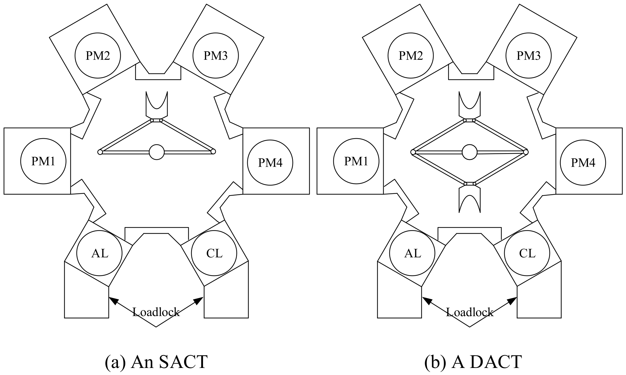
3.1. Reentrant Process

PMs in a cluster tool are divided into different groups. The PMs in the same group serve to perform the same fabrication operation called a step. For serial wafer flows, raw wafers sequentially visit several steps according to their processing recipes. For reentrant wafer flows (i.e., reentrant processes), wafers should revisit some steps multiple times. Notice that, for the steps involving reentrant processes, only one PM is configured so as to ensure processing consistency. For example, ALD and PECVD have such a requirement. Thus, if a wafer is repeatedly processed at a reentrant step, the processing environment is exactly identical such that the processing quality can be ensured.
There are three processing steps for the ALD process. After a raw wafer is moved out of an LL by the robot, the wafer is delivered to Step 1 to be processed, then Step 2, and followed by Step 3. When the processing of the wafer in Step 3 is completed, it revisits Steps 2 and 3 again such that a wafer visits Steps 2 and 3 totally k ≥ 2 times. Note that each step of Steps 2 and 3 has only one PM. In fact, the workloads at the reentrant steps are much greater than that in Step 1. Thus, more than one PM used for Step 1 cannot improve the productivity of a cluster tool. Therefore, only one PM is used to serve for Step 1 as well. Moreover, it can save cost to operate such a tool in this way since a PM (i.e., a chamber) is quite expensive. PMi, i ∈ {1, 2, 3}, is used for Step i. Then, the wafer flow pattern is denoted as (PM1, (PM2, PM3)k), with (PM2, PM3)k being the reentrant process.
Another commonly seen reentrant process is PECVD. For PECVD, it has two steps (i.e., Steps 1 and 2), and both are reentrant ones. PM1 is used to complete plasma-enhanced chemical vapor deposition in Step 1, while PM2 in Step 2 is used to complete a cure operation so as to ensure wafer quality. Then, (PM1, PM2)k, k ≥ 2, is used to represent the wafer flow pattern of PECVD. By observing the wafer flow patterns of ALD and PECVD, the reentrant pattern of PECVD is a special case of ALD from the perspective of scheduling. Thus, this work focuses on the scheduling analysis of DACTs with (PM1, (PM2, PM3)k) with k ≥ 2, which is commonly seen in cluster tool scheduling with reentrant processes. Note that the results in [5] are conducted for DACTs with (PM1, (PM2, PM3)k) as well.

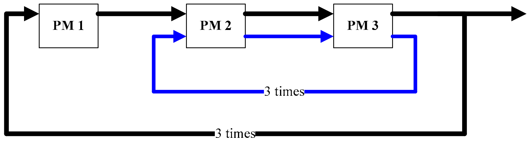
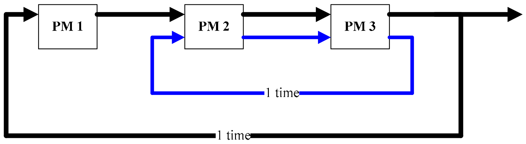
3.2. Activity Description

In a DACT, the two robot arms are named Arm-1 and Arm-2, respectively. Robot activities include picking a wafer from a PM, moving between two PMs, placing a wafer into a PM, rotating, and waiting. For a DACT, a swap strategy is efficient. At a state, assume that Arm-1 is empty and stays at PMi, while Arm-2 carries a wafer. At this state, a swap operation at PMi, i ∈ {1, 2, 3}, includes the following activities: Picking a processed wafer from PMi by Arm-1 → rotating → placing the wafer held by Arm-2 into PMi. The robot picking and placing activities at PMi are denoted as PIi and PLi, respectively. A swap operation at PMi is denoted as SWPi. Thus, SWPi includes PIi, robot rotation, and PLi. Besides, Mij is used to denote the robot moving from Steps i to j. Note that LLs are denoted as Step 0.
To model the time aspect, we assume that the time needed to execute each of the above-mentioned robot activities is constant. The activities of executing PIi, PLi, and Mij spend α, β, and μ time units, respectively. In practice, the time taken for SWPi is often less than the sum of the time for performing PIi, robot rotation, and PLi. Thus, symbol λ is introduced to represent the time needed for SWPi. Except for the robot activities, the wafer processing time at PMi, i ∈ {1, 2, 3}, is denoted as ρi. The meanings of the notations are summarized in Table 2.

3.3. Periodical Schedules

In a cluster tool, raw wafers enter the system one by one. The d-th wafer entering the system is denoted as Wd, d ∈ ℕ. To find a periodical schedule, it is necessary to analyze the state evolution of the system. Let Θi = {Wd(q)}, i ∈ {1, 2, 3}, denote the state of PMi (Step i), indicating that Wd is processed in PMi for the q-th operation. Furthermore, let Θ4 = {Ri(Wd(q)} denote the state of the robot, representing that the robot is staying at PMi, i ∈ {1, 2, 3}, and at the same time, carrying Wd with its q-th operation to be processed in the PM. Then, the state of the system is denoted as S = {Θ1, Θ2, Θ3, Θ4}.
For a DACT with (PM1, (PM2, PM3)2), by a swap strategy, Wu et al. [33] present a three-wafer periodical schedule called a 3-WP schedule in short. With a 3-WP schedule, starting from S1 = {W3(1), W2(2), W1(3), R1(W4(1))}, a DACT evolves as follows: S1 = {W3(1), W2(2), W1(3), R1(W4(1))} → S2 = {W4(1), W3(2), W1(3), R3(W2(3))} → S3 = {W4(1), W1(4), W2(3), R3(W3(3))} → S4 = {W4(1), W2(4), W3(3), R3(W1(5))} → S5 = {W4(1), W3(4), W1(5), R3(W2(5))} → S6 = {W4(1), W3(4), W2(5), R1(W5(1))} → S7 = {W5(1), W4(2), W3(5), R1(W6(1))} → S8 = {W6(1), W5(2), W4(3), R1(W7(1))} → S9 = {W7(1), W6(2), W4(3), R3(W5(3))}. Notice that S1 and S8 are equivalent. It implies that evolution from S1 to S8 forms a period.
Note that, to transfer S1 to S2 and S8 to S9, robot task sequence σ1 = 〈SWP1M12SWP2M23〉 is performed, i.e., the robot sequentially performs the following robot tasks: Swaps at PM1, moves to PM2 from PM1, swaps at PM2, and moves to PM3 from PM2. To transfer S2 to S3, σ2 = 〈SWP3M32SWP2M23〉 is performed, i.e., the robot sequentially performs the following robot tasks: Swaps at PM3, moves to PM2 from PM3, swaps at PM2, and moves to PM3 from PM2. σ2 is repeated for S3 to S4 and S4 to S5. Note that σ2 forms a robot task cycle involving the reentrant process (PM2, PM3)2, and it is called a local cycle. σ3 = 〈SWP3M30PL0PI0M01〉 is for S5 to S6. This means that the robot sequentially performs the following robot tasks for σ3: Swaps at PM3, moves to an LL from PM3, place a wafer into the LL, pick a wafer from the LL, and moves to PM1 from the LL. σ4 = 〈SWP1M12SWP2M23SWP3M30PL0PI0M01〉 is for S6 to S7 and S7 to S8. This means that the robot sequentially performs the following robot tasks for σ4: Swaps at PM1, moves to PM2 from PM1, swaps at PM2, moves to PM3 from PM2, swaps at PM3, moves to an LL from PM3, place a wafer into the LL, pick a wafer from the LL, and moves to PM1 from the LL. Obviously, σ4 is a robot cycle involving all PMs, and it is called a global cycle. Moreover, σ1 and σ3 together form a global cycle as well. Thus, as shown in Figure 2, a period from S1 to S8 (or S2 to S9) contains three local and three global cycles. Notice that, in each global cycle, one wafer with all operations being completed is returned to LLs. Thus, three wafers are returned to LLs in this period.
For a DACT with (PM1, (PM2, PM3)2), by a 3-WP schedule, as shown in Figure 2, Wu et al. [33] point out that the tool may operate under a transient process in some cases all the time. In such cases, once the robot enters the global cycles from local cycles, there might be a time delay when the robot arrives at the PMs involving reentrant processes. Such time delay makes that the lower bound of the system cycle time cannot be reached, i.e., a 1-WP schedule may not be optimal in such cases. This also implies that productivity reduction is caused by multiple local and global cycles in a period. Thus, it raises the question of whether the performance of the system can be improved by reducing the number of local and global cycles. To answer this question, for a DACT with (PM1, (PM2, PM3)2), Qiao et al. [5] present a 1-WP schedule.
By a 1-WP schedule, the tool should start to operate from a steady state, i.e., S1 = {W3(1), W1(4), W2(3), R1(W4(1))}. Then, by performing σ1, the system enters state S2 = {W4(1), W3(2), W2(3), R3(W1(5))}. Further, by executing σ2, it reaches S3 = {W4(1), W2(4), W1(5), R3(W3(3))}. Finally, by executing σ3, S4 = {W4(1), W2(4), W3(3), R1(W5(1))} is reached. At this time, S1 and S4 are equivalent. Thus, as shown in Figure 3, a period with a local and a global cycle is formed. Moreover, during such a period, a wafer is returned to LLs.
For a DACT with (PM1, (PM2, PM3)2), Qiao et al. [5] proved that the 1-WP schedule is optimal in terms of cycle time. However, in the cases where wafers are required to visit some PMs for k (>2) times, if there exists a value f ∈ ℕ = {1, 2 …} such that k = 3f holds, it is found that a 1-WP schedule cannot be obtained for a DACT, resulting in that the method in [5] is not applicable to such cases. It motivates us to conduct this work. Next, this work gives theoretical proofs for the above findings and provides the analytical expressions of the system cycle time if a 1-WP schedule exists for a DACT with (PM1, (PM2, PM3)k).

4. Scheduling Analysis by One-Wafer Cyclic Schedule

For a DACT with (PM1, (PM2, PM3)k), k ≥ 3, with a 3-WP schedule, the cycle time analysis has been conducted in [35]. It is found that there are (3k − 3) local cycles and three global cycles in a period. Thus, before a completed wafer goes back to LLs in a global cycle, it should undergo (3k − 3) local cycles to complete the reentrant process. Furthermore, when this wafer is returned to LLs, it has completed its (2k + 1)-th operation. Assume that a 1-WP schedule exists for a DACT with (PM1, (PM2, PM3)k). Then, the 1-WP schedule should result in a one-wafer period with multiple local cycles and a global cycle. Since only one completed wafer is returned to LLs in such a period, this wafer has already experienced (3k − 3) local cycles in fact. Notice that if (3k − 3) local cycles are consecutively performed, three wafers should be returned to LLs by three consecutive global cycles. This is a 3-WP schedule. If a 1-WP schedule exists, an obtained period should have (k − 1) local cycles first and then a global cycle such that a wafer is returned to LLs during each global cycle. Further, with a 1-WP schedule, there should be a state, i.e., S1 = {W1(1), W(ϑ1), W(2k + 1), R3(W(ϑ2))} at which the last local cycle in a period is just completed.
Theorem 1. 
For a DACT with (PM1, (PM2, PM3)k), if there exists a value f ∈ ℕ ∪ {0} such that k = 3f + 2 holds, then the system can be scheduled by a 1-WP schedule.
Proof. 
Starting from S1 = {W1(1), W(ϑ1), W(2k + 1), R3(W(ϑ2))}, S2 = {W2(1), W1(2), W(ϑ2), R3(W(ϑ1 + 1))} is reached after a global cycle. Thus, the tool then evolves in local cycles. After (k − 1) local cycles, the robot stays at PM3 and prepares to place W1 into PM3 for processing the (2f + 3)-th operation. Then, the tool undergoes a global cycle such that W1 is processed at PM3 for the (2f + 3)-th operation. Further, after (k − 1) local cycles, W1 is processed at PM2 for the (4f + 4)-th operation. In the next global cycle, the robot picks W1 from PM2 and moves to PM3, implying that the robot is going to place W1 into PM3 for processing the (4f + 5)-th operation. The following evolution also undergoes (k − 1) local cycles. After that, W1 is processed at PM3 for the (6f + 5)-th operation. Note that, the robot is staying at PM3 at this time. With k = 3f + 2, (6f + 5) = 2k + 1 holds. This means that W1 can be returned to LLs in the next global cycle. Further, by repeatedly performing (k − 1) local cycles and a global cycle, wafers (i.e., Wd, d ∈ ℕ\{1}) are continuously completed and returned to LLs. Hence, the system can be scheduled by a 1-WP schedule. □
In this case, for a DACT with (PM1, (PM2, PM3)k), k ≥ 2, if k is known and there exists a value f ∈ ℕ ∪ {0} such that k = 3f + 2 holds, Theorem 1 provides a simple way to find a state (i.e., S2 = {W2(1), W1(2), W(2f + 3), R3(W(4f + 5))}) starting from which a 1-WP schedule exists.
Theorem 2. 
For a DACT with (PM1, (PM2, PM3)k), if there exists a value f ∈ ℕ such that k = 3f holds, then the system cannot be scheduled by a 1-WP schedule.
Proof. 
Starting from marking S1 = {W1(1), W(ϑ1), W(2k + 1), R3(W(ϑ2))}, S2 = {W2(1), W1(2), W(ϑ2), R3(W(ϑ1 + 1))} is reached after a global cycle. Thus, the tool then evolves in local cycles. After (k − 1) local cycles, the robot is at PM3, and wafer W1 is just being processed at the PM for the (2f + 1)-th operation. By a 1-WP schedule, a global cycle should be performed next. In this global cycle, W1 should be delivered to LLs without completing all operations. Hence, the theorem holds. □
In this case, a 1-WP schedule is not applicable. Thus, this work presents two novel scheduling methods for this case in the next section to improve the system productivity.
Theorem 3. 
For a DACT with (PM1, (PM2, PM3)k), if there exists a value f ∈ ℕ such that k = 3f +1 holds, then the system can be scheduled by a 1-WP schedule.
Proof. 
Starting from S1 = {W1(1), W(ϑ1), W(2k + 1), R3(W(ϑ2))}, S2 = {W2(1), W1(2), W(ϑ2), R3(W(ϑ1 + 1))} is reached after a global cycle. Thus, the tool then evolves in local cycles. After (k − 1) local cycles, wafer W1 is just being processed at PM2 for the (2f + 2)-th operation. Then, after a global cycle, the robot picks W1 from PM2, moves to PM3, and stays there. By a 1-WP schedule, the following state evolution is for local cycles. After (k − 1) local cycles, the robot is at PM3 with W1 being held to be placed into the PM for the (4f + 3)-th operation. After the wafer is placed into the PM, W1 is processed in PM3 for the (4f + 3)-th operation, and then the system just enters the next global cycle. Then, after a global cycle, the system evolves for (k − 1) local cycles. After that, W1 is processed at PM3 for the (6f + 3)-th operation. Due to k = 3f + 1, (6f + 3) = 2k + 1 holds, implying that W1 can be returned to LLs in the next global cycle. Further, by repeatedly performing (k − 1) local cycles and a global cycle, wafers (i.e., Wd, d ∈ ℕ\{1}) are continuously completed and returned to LLs. Hence, the system can be scheduled by a 1-WP schedule. □
In this case, for a DACT with (PM1, (PM2, PM3)k), k ≥ 2, if k is known and there exists a value f ∈ ℕ such that k = 3f + 1 holds, Theorem 3 provides a simple way to find a state (i.e., S2 = {W2(1), W1(2), W(4f + 3), R3(W(2f + 3))}) starting from which a 1-WP schedule exists. Then, for the cases where a 1-WP schedule is applicable to a DACT with (PM1, (PM2, PM3)k), k ≥ 2, the cycle time is analyzed next.
For DACTs, in Step i (PMi), a swap operation makes a processed wafer removed from the PM and a new wafer placed into the PM. Then, the PM starts to process the wafer. When the robot comes to the PM again to perform a swap operation, the wafer in the PM is picked up, and a new wafer is placed into the PM again. Thus, the time taken to complete a wafer in Step i (i.e., the workload) is
Πi = ρi + λ, i ∈ {1, 2, 3}
Let φ and ψ denote the time taken for a local and a global cycle without considering the robot waiting time, respectively. Then, they can be calculated as follows.
φ = 2λ + 2μ
ψ = α + β + 3λ + 4μ
Further, let Πlocal = max{Π2, Π3, φ} and Π1-WP be the cycle time of a DACT with (PM1, (PM2, PM3)k), k ≥ 2, if a 1-WP schedule exists. Then, according to the cycle time analysis for a 1-WP schedule in [5], if Π1 ≤ (k − 1)Πlocal + ψ, Corollaries 1 and 2 are given below.
Corollary 1. 
For a DACT with (PM1, (PM2, PM3)k), when there does not exist a value f ∈ ℕ such that k = 3f holds, by a 1-WP schedule, if Π1 ≤ (k − 1)Πlocal + ψ and max{Π2, Π3} ≤ ψ, the cycle time is
Π1-WP = (k − 1)Πlocal + ψ
In fact, the time taken for the (k − 1) local cycles is (k − 1)Πlocal. In this case, due to Π1 ≤ (k − 1)Πlocal + ψ and max{Π2, Π3} ≤ ψ, when the robot comes to PMi, i ∈ {1, 2, 3}, the PM has completed the wafer processing. Thus, the robot can perform a swap operation immediately such that there is no robot waiting in the global cycle. Therefore, the time taken for the global cycle is ψ. Hence, in this case, (4) holds.
Corollary 2. 
For a DACT with (PM1, (PM2, PM3)k), when there does not exist a value f ∈ ℕ such that k = 3f holds, by a 1-WP schedule, if Π1 ≤ (k − 1)Πlocal + ψ and max{Π2, Π3} > ψ, the cycle time is
Π1-WP = local
In this case, due to Π1 ≤ (k − 1)Πlocal + ψ, it implies that when the robot comes to PM1, PM1 has completed the wafer processing. Thus, the robot can perform a swap operation immediately. However, due to max{Π2, Π3} > ψ, it implies that the time taken for the global cycle is max{Π2, Π3}. Therefore, (5) holds. Further, if Π1 > (k − 1)Πlocal + ψ, according to the cycle time analysis for a 1-WP schedule in [5], Corollaries 3–5 are given below.
Corollary 3. 
For a DACT with (PM1, (PM2, PM3)k), when there does not exist a value f ∈ ℕ such that k = 3f holds, by a 1-WP schedule, if kΠlocal ≥ Π1 > (k − 1)Πlocal +ψ and max{Π2, Π3} > ψ, the cycle time is
Π1-WP = local
In this case, due to Π1 > (k − 1)Πlocal + ψ, it implies that when the robot comes to PM1, the robot has to wait for some time since the PM has not completed the wafer processing yet at this time. The robot waiting time at PM1 should be Π1 − [(k − 1)Πlocal + ψ]. Without loss of generality, in this case, let Π3 = max{Π2, Π3} = Πlocal > ψ. This means that in a global cycle, the total robot waiting time should be Πlocalψ at least. Note that Π1 − [(k − 1)Πlocal + ψ] ≤ local − [(k − 1)Πlocal + ψ] = Πlocalψ, indicating that, in a global cycle, although the robot has waited at PM1 for Π1 − [(k − 1)Πlocal + ψ] time units, it still needs to wait at PM3 such that the time taken for the global cycle is Πlocal. Therefore, (6) holds.
Corollary 4. 
For a DACT with (PM1, (PM2, PM3)k), when there does not exist a value f ∈ ℕ such that k = 3f holds, by a 1-WP schedule, if Π1 > kΠlocal and max{Π2, Π3} > ψ, the cycle time is
Π1-WP = Π1
Corollary 5. 
For a DACT with (PM1, (PM2, PM3)k), when there does not exist a value f ∈ ℕ such that k = 3f holds, by a 1-WP schedule, if Π1 > (k − 1)Πlocal + ψ and max{Π2, Π3} ≤ ψ, the cycle time is
Π1-WP = Π1
For the cases given by Corollaries 4 and 5, in a global cycle, when the robot comes to PM1, the robot must wait there since the PM has not completed the wafer processing yet. However, when the robot comes to PMi, i ∈ {2, 3}, the wafer in the PM has been completed, meaning that the workload at PM1 dominates the system cycle time. Therefore, (7) and (8) for Corollaries 4 and 5 hold, respectively.
Besides, in the cases given by Corollaries 1–5, a 1-WP schedule can achieve the lower bound of the cycle time, i.e., it is optimal in terms of productivity. Up to now, the cycle time analysis has been done in all cases where a 1-WP schedule is applicable to a DACT with (PM1, (PM2, PM3)k). Based on the above analysis, to apply a 1-WP schedule, the key is to get the desired state of the system shown above, then, by starting from this state, the system can evolve with the 1-WP schedule.

5. Two Novel Scheduling Methods

As above-discussed, given the number k of revisiting times, if there is an f ∈ ℕ such that k = 3f, then no 1-WP schedule can be found. Thus, in this case, there is an issue of how to schedule the system so as to improve productivity. This section aims to tackle this issue by proposing two novel scheduling methods.
For a DACT with (PM1, (PM2, PM3)k), k ≥ 2, when the system evolves from local cycles to a global cycle, there might be wafer delay time in PMs involved in the reentrant process in the global cycle such that the system cycle time cannot reach its lower bound [33]. Thus, after the local cycles, if the number of global cycles can be decreased, the system cycle time can be improved. With this idea, the first scheduling method is proposed.

5.1. Scheduling Method One

Without loss of generality, the scheduling analysis is conducted for a DACT with (PM1, (PM2, PM3)3). Then, by the proposed method, a DACT with (PM1, (PM2, PM3)3) evolves as follows: S1 = {W4(1), W3(2), W1(5), R3(W2(5))} → S2 = {W4(1), W1(6), W2(5), R3(W3(3))} → S3 = {W4(1), W2(6), W3(3), R3(W1(7))} → S4 = {W4(1), W3(4), W1(7), R3(W2(7))} → S5 = {W5(1), W4(2), W2(7), R3(W3(5))} → S6 = {W6(1), W5(2), W3(5), R3(W4(3))} → S7 = {W6(1), W3(6), W4(3), R3(W5(3))} → S8 = {W6(1), W4(4), W5(3), R3(W3(7))} → S9 = {W6(1), W5(4), W3(7), R3(W4(5))} → S10 = {W7(1), W6(2), W4(5), R3(W5(5))} with S1 and S10 being equivalent. Thus, a period from S1 to S10 is formed. Note that to reach S2 from S1, S3 from S2, S4 from S3, S7 from S6, S8 from S7, and S9 from S8, robot task sequence σ2 for a local cycle is performed, respectively. To reach S5 from S4, S6 from S5, and S10 from S9, σ5 = 〈SWP3M30PL0PI0M01SWP1M12SWP2M23〉 is executed, respectively. Note that σ5 is a global cycle.
During a period from S1 to S10, before two global cycles (i.e., the first global cycle from S4 to S5 and the second one from S5 to S6), three local cycles are performed at first. Then, there are three local cycles again, and they are followed by one global cycle (i.e., the third global cycle from S9 to S10). Thus, after the local cycles, the number of global cycles followed is decreased by comparing with the 3-WP schedule presented in [33,35]. Moreover, in each global cycle, one wafer is returned to LLs. Totally, three wafers are returned to LLs in a period. Therefore, it is also a 3-WP schedule. However, it is different from the 3-WP schedule presented in [33,35], by which three wafers are completed in three consecutive global cycles in a period. Thus, it is a new 3-WP schedule, called an N3-WP1 schedule in short. Let ΠN3-WP1 denote the system cycle time by an N3-WP1 schedule.
Theorem 4. 
For a DACT with (PM1, (PM2, PM3)3), by an N3-WP1 schedule, if Π1 ≤ 3Πlocal + ψ and max{Π2, Π3} ≤ ψ, the cycle time is
Π N 3 - WP 1 = 2 Π l o c a l + ψ ,   i f   ψ     Π 1 6 Π l o c a l + 2 ψ + Π 1 3 ,   i f   ψ < Π 1
Proof. 
From S1 to S4, there are three local cycles that take 3Πlocal time units. After that, the system performs two global cycles. Due to Π1 ≤ 3Πlocal + ψ and max{Π2, Π3} ≤ ψ, when the robot arrives at PMi, i ∈ {1, 2, 3}, to pick up a wafer in the first global cycle from S4 to S5, the wafer should have been processed and can be picked up from the PM immediately. Therefore, the robot does not need to wait at PMi, i ∈ {1, 2, 3}, such that ψ time units are needed for the first global cycle. Then, if ψ < Π1, the next global cycle from S5 to S6 takes Π1 time units, and otherwise, it takes ψ time units. From S6 to S9, the three local cycles take 3Πlocal time units. For the global cycle from S9 to S10, ψ time units are required due to Π1 ≤ 3Πlocal + ψ. Thus, by an N3-WP1 schedule, if ψΠ1, a period takes 6Πlocal + 3ψ time units, and otherwise it takes 6Πlocal + 2ψ + Π1 time units. Therefore, (9) holds. □
In this case, when ψ < Π1, the result obtained by a 3-WP schedule is improved. Let ω1i, ω2i, and ω3i, i ∈ {1, 2, 3}, denote the robot waiting time before a swap operation at PM1, PM2 and PM3 in the i-th global cycle in a period, respectively. Moreover, let χ = Π1Πlocal. The following result is achieved.
Theorem 5. 
For a DACT with (PM1, (PM2, PM3)3), by an N3-WP1 schedule, if Π1 ≤ 3Πlocal + ψ and max{Π2, Π3} > ψ, the cycle time is
Π N 3 - W P 1 = 3 Π l o c a l ,   i f   Π l o c a l ψ     χ 3 Π l o c a l + χ + ψ Π l o c a l 3 ,   i f   Π l o c a l ψ < χ
Proof. 
By Theorem 4, for the three local cycles from S1 to S4, 3Πlocal time units are required. After that, the system undergoes two global cycles. Due to Π1 ≤ 3Πlocal + ψ, when the robot arrives at PM1 to pick up a wafer in the first global cycle from S4 to S5, the wafer should have been processed and can be picked up from the PM immediately. Therefore, ω11 = 0. Further, due to max{Π2, Π3} > ψ, ω21 + ω31 = Πlocalψ. In this way, the wafer in a PM with a higher workload of PM2 and PM3 can be picked up once it is processed. Thus, Πlocal time units are needed for the first global cycle. In the second global cycle from S5 to S6, when the robot comes to PM1, there are two cases: (1) Πlocalψχ and (2) Πlocalψ < χ. In the first case, before the robot can pick a wafer up from PM1, it should wait at the PM for ω12 = Π1 − (ψ + ω21 + ω31) = Π1Πlocal = χ time units if χ ≥ 0, or ω12 = 0 if χ < 0. Then, due to max{Π2, Π3} > ψ, ω22 + ω32 = Πlocalψω12 = Πlocalψmax(χ, 0) ≥ 0, implying that a wafer in a PM with the higher workload of PM2 and PM3 can be picked up once it is processed. Thus, the time taken for the second global cycle is Πlocal in this case. In Case (2), before the robot can pick a wafer up from PM1, it should wait at the PM for ω12 = Π1 − (ψ + ω21 + ω31) = Π1Πlocal = χ > Πlocalψ > 0 time units. Further, when the robot comes to PM2 or PM3 to pick up a wafer, the wafer has already been processed due to Πlocalψ < χ = ω12 (i.e., Πlocal < ω12 + ψ). Thus, for the second global cycle, it spends ω12 + ψ = χ + ψ time units. Similarly, the time taken for the process from S6 to S10 is 4Πlocal. Hence, (10) holds. □
In this case, when Πlocalψ ≥ χ, the cycle time is optimal. Furthermore, when Πlocalψ < χ, the result obtained by a 3-WP schedule is improved.
Theorem 6. 
For a DACT with (PM1, (PM2, PM3)3), by an N3-WP1 schedule, if 4Πlocal ≥ Π1 > 3Πlocal + ψ and max{Π2, Π3} > ψ, the cycle time is
ΠN3-WP1 = (Π1 + 7Πlocal + ψ + max{2Π1ψ − 7Πlocal, 0})/3
Proof. 
Note that in the second global cycle from S5 to S6, due to Π1 > 3Πlocal + ψ, ω22 + ω32 = 0 should hold. Thus, from S6 to S10, it takes 4Πlocal time units due to 4ΠlocalΠ1 > 3Πlocal + ψ and max{Π2, Π3} > ψ. Further, in the third global cycle, ω13 = Π1 − (3Πlocal + ψ) and ω23 + ω33 = Πlocalω13ψ = 4ΠlocalΠ1.
By Theorem 4, from S1 to S4, it takes 3Πlocal time units. Further, with ω23 + ω33 = 4ΠlocalΠ1, during the first global cycle from S4 to S5, ω11 = max(Π1 − (3Πlocal + ψ) − (ω23 + ω33), 0) = max(Π1 − (3Πlocal + ψ) − (4ΠlocalΠ1), 0) = max{2Π1ψ − 7Πlocal, 0} and ω21 + ω31 = Πlocalψmax{2Π1ψ − 7Πlocal, 0}. If 2Π1ψ − 7Πlocal > 0, then Πlocalψmax{2Π1ψ − 7Πlocal, 0} = Πlocalψ − 2Π1 + ψ + 7Πlocal = 8Πlocal − 2Π1 ≥ 0, i.e., ω21 + ω31 ≥ 0. Therefore, the time taken for the first global cycle is ψ + ω11 + ω21 + ω31 = Πlocal.
In the second global cycle from S5 to S6, ω12 = Π1Πlocal + max{2Π1ψ − 7Πlocal, 0} > 2Πlocal + ψ + max{2Π1ψ − 7Πlocal, 0} holds due to Π1 > 3Πlocal + ψ. Thus, ω22 + ω32 = 0. Therefore, the time taken for this global cycle is ω12 + ψ = Π1Πlocal + max{2Π1ψ − 7Πlocal, 0} + ψ.
Thus, the time taken for a period from S1 to S10 is Π1 + 7Πlocal + ψ + max{2Π1ψ − 7Πlocal, 0}. With three wafers being completed in a period, the cycle time can be obtained by (11). □
Similar to Corollaries 4 and 5, the following two theorems are presented. Due to the space limit, their proofs are omitted.
Theorem 7. 
For a DACT with (PM1, (PM2, PM3)3), by an N3-WP1 schedule, if Π1 > 4Πlocal and max{Π2, Π3} > ψ, the cycle time is
ΠN3-WP1 = Π1
Theorem 8. 
For a DACT with (PM1, (PM2, PM3)3), by an N3-WP1 schedule, if Π1 > 3Πlocal + ψ and max{Π2, Π3} ≤ ψ, the cycle time is
ΠN3-WP1 = Π1
Note that in the cases presented by Theorems 7 and 8, the cycle time is optimal.

5.2. Scheduling Method Two

Up to now, the cycle time analysis for a DACT with (PM1, (PM2, PM3)3) by an N3-WP1 schedule has been done. With the N3-WP1 schedule, in some cases, the productivity of the system is improved over the existing 3-WP schedule. However, in some other cases, the optimal cycle time cannot be achieved. Thus, we present another scheduling method by which a DACT with (PM1, (PM2, PM3)3) evolves as follows: S1 = {W4(1), W3(2), W2(3), R3(W1(7))} → S2 = {W4(1), W2(4), W1(7), R3(W3(3))} → S3 = {W5(1), W4(2), W3(3), R3(W2(5))} → S4 = {W5(1), W3(4), W2(5), R3(W4(3))} → S5 = {W5(1), W2(6), W4(3), R3(W3(5))} → S6 = {W5(1), W4(4), W3(5), R3(W2(7))} → S7 = {W5(1), W3(6), W2(7), R3(W4(5))} → S8 = {W6(1), W5(2), W4(5), R3(W3(7))} → S9 = {W6(1), W4(6), W3(7), R3(W5(3))} → S10 = {W7(1), W6(2), W5(3), R3(W4(7))}. Since S1 and S10 are equivalent, a period is formed by this state evolution. In the above state evolution, to realize the process from S1 to S2, S3 to S4, S4 to S5, S5 to S6, S6 to S7, and S8 to S9, robot task sequence σ1 for a local cycle is executed, respectively, while to reach S3 from S2, S8 from S7, and S10 from S9, robot task sequence σ5 for a global cycle is executed, respectively.
During the period from S1 to S10, at first, there is a local cycle followed by a global cycle (i.e., the first global cycle from S2 to S3). Then, there are four local cycles and then a global cycle (i.e., the second global cycle from S7 to S8) is followed. After that, there is a local cycle followed by a global cycle (i.e., the third global cycle from S9 to S10) again. In each global cycle, one wafer is completed. Thus, during the period, it is also a 3-WP schedule that is different from the one presented in [33,35]. In this work, the second scheduling method is called an N3-WP2 schedule in short. Let ΠN3-WP2 denote the system cycle time under an N3-WP2 schedule. Based on Corollary 1 and Theorem 4, we present Theorem 9, while based on Corollary 2 and Theorem 5, we can get Theorem 10. The proofs of Theorems 9 and 10 are omitted due to the space limit.
Theorem 9. 
For a DACT with (PM1, (PM2, PM3)3), by an N3-WP2 schedule, if Π1 ≤ Πlocal + ψ and max{Π2, Π3} ≤ ψ, the cycle time is
ΠN3-WP2 = 2Πlocal + ψ
Theorem 10. 
For a DACT with (PM1, (PM2, PM3)3), by an N3-WP2 schedule, if Π1 ≤ Πlocal + ψ and max{Π2, Π3} > ψ, the cycle time is
ΠN3-WP2 = 3Πlocal
In these two cases, as presented in Theorems 9 and 10, the cycle time cannot be shortened anymore, implying that this is the lower bound. For an N3-WP2 schedule, ω1i, ω2i, and ω3i, I ∈ {1, 2, 3}, are also used to denote the robot waiting time before a swap operation at PM1, PM2, and PM3 in the i-th global cycle during a period, respectively. Then, the following result is presented.
Theorem 11. 
For a DACT with (PM1, (PM2, PM3)3), by an N3-WP2 schedule, if 2Πlocal ≥ Π1 > Πlocal + ψ and max{Π2, Π3} > ψ, the cycle time is
ΠN3-WP2 = 3Πlocal
Proof. 
Due to 2ΠlocalΠ1 > Πlocal + ψ, the time taken for the state evolution from S3 to S8 is 5Πlocal. Further, ω22 + ω32 = 0 holds. For the local cycle from S8 to S9, it takes Πlocal time units. In the global cycle from S9 to S10, when the robot comes to PM1, due to Π1 > Πlocal + ψ, it has to wait there for ω13 = Π1 − (Πlocal + ψ) time units. Further, we have ω23 + ω33 = Πlocalψω13 = 2ΠlocalΠ1 ≥ 0. Then, the time taken for the global cycle from S9 to S10 is ψ + ω13 + ω23 + ω33 = Πlocal. Similarly, for the local cycle from S1 to S2, it takes Πlocal time units. For the global cycle from S2 to S3, when the robot comes to PM1, due to Π1 > Πlocal + ψ, it has to wait there for ω11 = max(Π1 − (Πlocal + ψ) − (ω23 + ω33), 0) = max(Π1 − (Πlocal + ψ) − (2ΠlocalΠ1), 0) = max(2Π1 − 3Πlocalψ, 0) time units. Then, there are two cases: (1) ω11 = 0 and (2) ω11 = 2Π1 − 3Πlocalψ. In Case (1), ω21 + ω31 = Πlocalψ, leading to that the time taken for the global cycle from S2 to S3 is ψ + ω11 + ω21 + ω31 = Πlocal. In Case (2), ω21 + ω31 = Πlocalψω11 = Πlocalψ − (2Π1 − 3Πlocalψ) = 4Πlocal − 2Π1 ≥ 0 due to 2ΠlocalΠ1. Thus, in this case, the time taken for the global cycle from S2 to S3 is ψ + ω11 + ω21 + ω31 = Πlocal as well. Therefore, it takes 9Πlocal time units for the period from S1 to S10. With three wafers completed in the period, (16) holds. □
The cycle time cannot be shortened in this case either, i.e., it is optimal. Further, the following result for another case can be obtained.
Theorem 12. 
For a DACT with (PM1, (PM2, PM3)3), by an N3-WP2 schedule, if 4Πlocal ≥ Π1 > 2Πlocal and max{Π2, Π3} > ψ, the cycle time is
Π N 3 - W P 2 = 3 Π l o c a l ,   i f   5 Π l o c a l 2 Π 1 ψ     0 4 Π l o c a l + ψ + 2 Π 1 3 ,   i f   5 Π l o c a l 2 Π 1 ψ < 0
Proof. 
For the four local cycles from S3 to S7, it takes 4Πlocal time units. With 4ΠlocalΠ1 > 2Πlocal, 4Πlocal + ψ > Π1 holds. Thus, during the global cycle from S7 to S8, when the robot comes to PM1, the robot does not need to wait before swapping at the PM, i.e., ω12 = 0. Further, ω22 + ω32 = Πlocalψ, resulting in that the time taken for the global cycle from S7 to S8 is ψ + ω12 + ω22 + ω32 = Πlocal. For the local cycle from S8 to S9, it takes Πlocal time units. In the global cycle from S9 to S10, when the robot comes to PM1, it has to wait there for ω13 = Π1Πlocalψ − (ω22 + ω32) = Π1 − 2Πlocal > 0 time units due to 4ΠlocalΠ1 > 2Πlocal. Further, we have ω23 + ω33 = max(Πlocal − (ω13 + ψ), 0) = max(Πlocal − (Π1 − 2Πlocal + ψ), 0) = max(3ΠlocalΠ1ψ, 0). Then, there are two cases as follows.
Case 1: max(3ΠlocalΠ1ψ, 0) = 3ΠlocalΠ1ψ. In this case, the time taken for the global cycle from S9 to S10 is ψ + ω13 + ω23 + ω33 = ψ + Π1 − 2Πlocal + 3ΠlocalΠ1ψ = Πlocal. Then, the time taken for the local cycle from S1 to S2 is Πlocal. Furthermore, in the global cycle from S2 to S3, when the robot arrives at PM1, it has to wait there for ω11 = Π1Πlocalψ − (ω23 + ω33) = Π1Πlocalψ − (3ΠlocalΠ1ψ) = 2Π1 − 4Πlocal > 0 time units due to 4ΠlocalΠ1 > 2Πlocal. Thus, ω21 + ω31 = max(Πlocal − (ω11 + ψ), 0) = max(Πlocal − (2Π1 − 4Πlocal + ψ), 0) = max(5Πlocal − 2Π1ψ, 0). Then, there are two cases as follows again. Case 1.1: max(5Πlocal − 2Π1ψ, 0) = 5Πlocal − 2Π1ψ. In this case, the time taken for the global cycle S2 to S3 is ψ + ω11 + ω21 + ω31 = ψ + 2Π1 − 4Πlocal + 5Πlocal − 2Π1ψ = Πlocal. Hence, the time taken for a period from S1 to S10 is 9Πlocal in this case. Case 1.2: max(5Πlocal − 2Π1ψ, 0) = 0. In this case, the time taken for the global cycle from S2 to S3 is ψ + ω11 + ω21 + ω31 = ψ + 2Π1 − 4Πlocal. Hence, the time taken for a period from S1 to S10 is 4Πlocal + ψ + 2Π1 in this case.
Case 2: max(3ΠlocalΠ1ψ, 0) = 0. In this case, the time taken for the global cycle from S9 to S10 is ψ + ω13 + ω23 + ω33 = ψ + Π1 − 2Πlocal. Then, the time taken for the local cycle from S1 to S2 is Πlocal. Furthermore, in the global cycle from S2 to S3, when the robot arrives at PM1, it has to wait there for ω11 = Π1Πlocalψ − (ω23 + ω33) = Π1Πlocalψ > 0 time units. Thus, ω21 + ω31 = max(Πlocal − (ω11 + ψ), 0) = max(2ΠlocalΠ1, 0) = 0. Therefore, the time taken for the global cycle from S2 to S3 is ψ + ω11 + ω21 + ω31 = Π1Πlocal. Hence, the time taken for a period from S1 to S10 is 4Πlocal + ψ + 2Π1 in this case.
In summary, we conclude that the theorem holds. □
Therefore, by an N3-WP2 schedule, we ensure that, in the case with 5Πlocal − 2Π1ψ ≥ 0, the cycle time is optimal. Further, by Theorem 12, the following result can be obtained.
Theorem 13. 
For a DACT with (PM1, (PM2, PM3)3), by an N3-WP2 schedule, if 3Πlocal + ψ ≥ Π1 > Πlocal + ψ and max{Π2, Π3} ≤ ψ, the cycle time is
ΠN3-WP2 = (4Πlocal + 2Π1 + ψ)/3
Proof. 
For the four local cycles from S3 to S7, it takes 4Πlocal time units. With 3Πlocal + ψΠ1, 4Πlocal + ψ > Π1 holds. Thus, during the global cycle from S7 to S8, when the robot comes to PM1, the robot does not need to wait before swapping at the PM, i.e., ω12 = 0. Further, ω22 + ω32 = 0 due to max{Π2, Π3} ≤ ψ. Therefore, the time taken for the global cycle from S7 to S8 is ψ. For the local cycle from S8 to S9, it takes Πlocal time units. During the global cycle from S9 to S10, when the robot comes to PM1, it has to wait there for ω13 = Π1Πlocalψ − (ω22 + ω32) = Π1Πlocalψ > 0 time units. Further, ω23 + ω33 = 0 due to max{Π2, Π3} ≤ ψ. Thus, the time taken for the global cycle from S9 to S10 is ψ + ω13 + ω23 + ω33 = Π1Πlocal. Similarly, the time taken for the local cycle from S1 to S2 and the global cycle from S2 to S3 is Πlocal and Π1Πlocal, respectively. Thus, the time taken for the period from S1 to S10 is 4Πlocal + ψ + 2Π1. Therefore, with three wafers being completed in such a period, the cycle time can be obtained by (18), or the theorem holds. □
Based on the above development, Algorithm 1 is presented to determine one of the schedules N3-WP1 and N3-WP2 to be applied to the system to maximize productivity.
Algorithm 1: For a DACT with (PM1, (PM2, PM3)3), the following algorithm is applied to choose one of the N3-WP1 and N3-WP2 schedules for the tool.
Input: ρ1, ρ2, ρ3, α, μ, β, and λ
Output: The adopted schedule
1.Calculate ψ, Π1, Π2, Π3, and Πlocal;
2.If max{Π2, Π3} ≤ ψ
3.If Π1Πlocal + ψ
4.  The N3-WP2 schedule is applied, and the cycle time is calculated by Theorem 9;
5.If Πlocal + ψ < Π1 ≤ 3Πlocal + ψ
6.  Calculate ΠN3-WP1 by Theorem 4 and ΠN3-WP2 by Theorem 13;
7.  If ΠN3-WP1 < ΠN3-WP2
8.   The N3-WP1 schedule is applied;
9.   Else
10.   The N3-WP2 schedule is applied;
11.If Π1 > 3Πlocal + ψ
12.  The N3-WP1 schedule is applied, and the cycle time is calculated by Theorem 8;
13.Else
14.If Π1Πlocal + ψ
15.  The N3-WP2 schedule is applied, and the cycle time is calculated by Theorem 10;
16.If Πlocal + ψ < Π1 ≤ 2Πlocal
17.  The N3-WP2 schedule is applied, and the cycle time is calculated by Theorem 11;
18.If 2Πlocal < Π1 ≤ 2.5Πlocal − 0.5ψ
19.  The N3-WP2 schedule is applied, and the cycle time is calculated by Theorem 12;
20.If 2.5Πlocal − 0.5ψ < Π1 ≤ 3Πlocal + ψ
21.  Calculate ΠN3-WP1 by Theorem 5 and ΠN3-WP2 by Theorem 12;
22.  If ΠN3-WP1 < ΠN3-WP2
23.   The N3-WP1 schedule is applied;
24.   Else
25.   The N3-WP2 schedule is applied;
26.If 3Πlocal + ψ < Π1 ≤ 4Πlocal
27.  Calculate ΠN3-WP1 by Theorem 6 and ΠN3-WP2 by Theorem 12.
28.  If ΠN3-WP1 < ΠN3-WP2
29.   The N3-WP1 schedule is applied;
30.   Else
31.   The N3-WP2 schedule is applied;
32.If Π1 > 4Πlocal
33.  The N3-WP1 schedule is applied, and the cycle time can be obtained by Theorem 7;
Note that, in the case with 4Πlocal < Π1 and max{Π2, Π3} > ψ, by Theorem 7, an N3-WP1 schedule can achieve the minimum system cycle time, while in the case with Π1 > 3Πlocal + ψ and max{Π2, Π3} ≤ ψ, by Theorem 8, an N3-WP1 schedule can achieve the minimum system cycle time as well. Thus, we do not present the cycle time analysis in both cases under an N3-WP2 schedule. Now, we have completed the cycle time analysis for a DACT with (PM1, (PM2, PM3)3) by the N3-WP1 and N3-WP2 schedules.
Based on Theorems 10–12, in the case with 2.5Πlocal − 0.5ψΠ1 and max{Π2, Π3} > ψ, an N3-WP2 schedule is optimal. Based on Theorem 7, in the case with Π1 > 4Πlocal and max{Π2, Π3} > ψ, an N3-WP1 schedule is optimal. Based on Theorem 9, in the case with Π1Πlocal + ψ and max{Π2, Π3} ≤ ψ, an N3-WP2 schedule is optimal. Based on Theorem 8, in the case with Π1 > 3Πlocal + ψ and max{Π2, Π3} ≤ ψ, an N3-WP1 schedule is optimal. In other cases, for the N3-WP1 and N3-WP2 schedule, the one with the minimum cycle time can be applied to a DACT with (PM1, (PM2, PM3)3). This is what Algorithm 1 does. Besides, in such cases, the adopted scheduling method cannot ensure optimality in terms of the cycle time. This is also the limitation of this work.
Note that by extending the N3-WP1 and N3-WP2 schedules, similar schedules can be developed for a DACT with (PM1, (PM2, PM3)k), k ∈ {3f| f ∈ ℕ\{1}}. Furthermore, the cycle time can be analyzed in a similar way. Besides, according to the investigation from enterprises of integrated circuit high-end technological equipment, for DACTs with k-time reentrant processes, k is normally no greater than five. Therefore, the obtained results in this work match the practical demand well.

6. Implementation of the Proposed Methods and Illustrative Examples

6.1. Implementation of the Proposed Methods

For a DACT with (PM1, (PM2, PM3)k), k ≥ 2 and k ≠ 3f, f ∈ {1, 2 …}, based on Theorems 1 and 3, a 1-WP schedule exists for the tool such that the lower bound of the system cycle time can be achieved. Let W0 denote a virtual wafer and assume that a tool starts from its idle state. To implement the 1-WP schedule for a DACT, virtual wafers are introduced into the tool, and we assume that at the initial state, each PM is processing a virtual wafer and also the robot is holding a wafer.
For the case that a DACT with (PM1, (PM2, PM3)k), k = 3f +2 and f ∈ ℕ ∪ {0}, Theorem 1 provides a simple way to find a state (i.e., {W2(1), W1(2), W(2f + 3), R3(W(4f + 5))}) starting from which a 1-WP schedule exists. By introducing virtual wafers into the tool, let S0 = {W0(1), W0(2), W0(3), R3(W0(5))} be the initial (idle) state of the tool. Then, by the swap strategy, the tool can evolve into a state in which all virtual wafers are removed from the tool. At this time, the wafers in the tool are all real ones. In this way, the 1-WP schedule is implemented.
For the case that a DACT with (PM1, (PM2, PM3)k), k = 3f +1 and f ∈ ℕ, Theorem 3 provides a simple way to find a state (i.e., {W2(1), W1(2), W(4f + 3), R3(W(2f + 3))}) starting from which a 1-WP schedule exists. By introducing virtual wafers into the tool, let S0 = {W0(1), W0(2), W0(7), R3(W0(5))} be the initial (idle) state of the tool. Then, by the swap strategy, the tool can evolve into a state in which all virtual wafers are removed from the tool, and the wafers in the tool are all real ones. In this way, the 1-WP schedule is implemented.
For a DACT with (PM1, (PM2, PM3)k), k = 3f and f ∈ ℕ, based on Theorem 2, a 1-WP schedule does not exist. In this case, this work presents two methods (an N3-WP1 schedule and an N3-WP2 schedule) to operate the tool for productivity improvement. To implement the N3-WP1 schedule, by introducing virtual wafers, let S0 = {W0(1), W0(2), W0(5), R3(W0(5))} be the initial (idle) state of the tool. Then, by the swap strategy, the tool can evolve into a state in which all virtual wafers are removed from the tool, and the wafers in the tool are all real ones. To implement the N3-WP2 schedule, by introducing virtual wafers, let S0 = {W0(1), W0(2), W0(3), R3(W0(7))} be the initial (idle) state of the tool. Then, by the swap strategy, the tool can evolve into a state in which all virtual wafers are removed from the tool, and the wafers in the tool are all real ones. In this way, the N3-WP1 schedule and N3-WP2 schedule are implemented.

6.2. Illustrative Examples

Now, several examples are presented to demonstrate the obtained results in this work. Among them, Examples 2–4 come from [35]. Note that Π3-WP represents the system cycle time obtained by a 3-WP schedule.
Example 1. 
For a DACT with (PM1, (PM2, PM3)5), the wafer processing time at PM1, PM2, and PM3 is 80 s, 35 s, and 50 s (i.e., ρ1 = 80 s, ρ2 = 35 s, and ρ3 = 50 s), respectively, and α = μ = β = 3 s and λ = 8 s.
For this example, k = 3 × 1 + 2 with f = 1, Π1 = 88 s, Π2 = 43 s, Π3 = 58 s, and ψ = 42 s. By applying a 3-WP schedule, Π3-WP = (290 + 44/3) s ≈ 304.67 s. However, if a 1-WP schedule is applied, it follows from Corollary 2 that Π1-WP = 5Π3 = 290 s. Obviously, the 1-WP schedule outperforms the 3-WP schedule.
Example 2. 
For a DACT with (PM1, (PM2, PM3)3), ρ1 = 37 s, ρ2 = 22 s, ρ3 = 32 s, α = μ = β = 4 s, and λ = 8 s.
For this example, Π1 = 45 s, Π2 = 30 s, Π3 = 40 s, and ψ = 48 s. By using a 3-WP schedule, we get Π3-WP = 128 s. If an N3-WP1 schedule is applied, by Theorem 4, we get ΠN3-WP1 = 128 s, while if an N3-WP2 schedule is applied, by Theorem 9, we also get ΠN3-WP2 = 128 s. Thus, the three scheduling methods can obtain the same results.
Example 3. 
For a DACT with (PM1, (PM2, PM3)3), ρ1 = 50 s, ρ2 = 22 s, ρ3 = 32 s, α = μ = β = 4 s, and λ = 8 s.
For this example, Π1 = 58 s, Π2 = 30 s, Π3 = 40 s, and ψ = 48 s. By using a 3-WP schedule, Π3-WP = 404/3 s ≈ 134.67 s. However, if an N3-WP1 schedule is applied, by Theorem 4, ΠN3-WP1 = 394/3 s ≈ 131.33 s. If an N3-WP2 schedule is applied, by Theorem 9, ΠN3-WP2 = 128 s. Thus, in this case, an N3-WP2 schedule should be applied since it can achieve the best performance among the three schedules.
Example 4. 
For a DACT with (PM1, (PM2, PM3)3), ρ1 = 450 s, ρ2 = 200 s, ρ3 = 250 s, α = μ = β = 3 s, and λ = 8 s.
For this example, Π1 = 458 s, Π2 = 208 s, Π3 = 258 s, and ψ = 42 s. By using a 3-WP schedule, Π3-WP = (774 + 184/3) s ≈ 835.33 s. However, if an N3-WP1 schedule is applied, by Theorem 5, ΠN3-WP1 = 774 s. If an N3-WP2 schedule is applied, by Theorem 11, ΠN3-WP2 = 774 s. Thus, in this case, we can choose either N3-WP1 or N3-WP2 to improve the cycle time by 7.34% in comparison with a 3-WP schedule.
Example 5. 
For a DACT with (PM1, (PM2, PM3)3), ρ1 = 200 s, ρ2 = 45 s, ρ3 = 50 s, α = μ = β = 2 s, and λ = 5 s.
In this example, Π1 = 205 s, Π2 = 50 s, Π3 = 55 s, and ψ = 27 s. By using a 3-WP schedule, we have Π3-WP = (165 + 272/3) s ≈ 255.67 s. However, if an N3-WP1 schedule is applied, by Theorem 6, ΠN3-WP1 = 617/3 s ≈ 205.67 s. If an N3-WP2 schedule is applied, by Theorem 12, ΠN3-WP2 = 219 s. Thus, in this case, the N3-WP1 schedule should be applied, and it improves the cycle time by 19.56% in comparison with a 3-WP schedule.
In Examples 1–5, with the parameters of the cluster tool provided, we can quickly obtain the cycle time of the system under any one of the 3-WP schedule, N3-WP1 schedule, N3-WP2 schedule, and 1-WP schedule (if existing). With the system cycle time obtained, one can determine the best scheduling method to be applied to DACTs with reentrant wafer flows.
Besides, more examples are given in Table 3 to show the superiority of the proposed methods by comparing them with the 3-WP schedule in terms of the system cycle time. In the cases in Table 3, the time for the robot activities and wafer processing is set according to real applications in a semiconductor equipment vendor in China. With these given parameters of cluster tools, Algorithm 1 can be used to obtain the best scheduling method immediately in the cases shown in Table 3. Furthermore, by using the best one of the N3-WP1 and N3-WP2 schedules, the cycle time of the system is improved by 16.8% on average by comparing with the 3-WP schedule. Besides, in Cases 1–6, the adopted scheduling method can achieve a minimal cycle time. However, in Cases 7–11, the optimality of the adopted scheduling method cannot be ensured. Nevertheless, the adopted method significantly outperforms the existing 3-WP schedule.

7. Conclusions

Wafer reentrant flows normally exist for some processes, such as chemical vapor and physical vapor deposition. Moreover, cluster tools are widely applied to wafer fabrication for such processes. Such a tool compactly integrates several PMs, a wafer transport robot, and two LLs. It can provide a highly precise vacuum environment for wafer fabrication. Since there is no buffer between PMs, it is important to effectively schedule such a tool with reentrant processes. For a DACT with two-time reentrant processes, it is found that a 1-WP schedule can achieve the optimal cycle time. However, for some wafer fabrication processes, wafers should be processed at some processing steps more than two times. Up to now, the problem is open for the issue if a 1-WP schedule exists for a DACT with wafer reentrant processes for more than two times. If not, it raises the question of whether a better schedule exists by comparing it with an existing 3-WP schedule. This motivates us to do this work to answer this question.
In this work, theorical analysis is conducted on it. In Section 4, it is shown that if there exists a value f ∈ ℕ such that k = 3f holds, then a 1-WP schedule does not exist, and otherwise, the system can be scheduled by a 1-WP schedule. Further, analytical expressions are given to calculate the system cycle time if a 1-WP schedule exists. In the cases where a 1-WP schedule is not applicable, this work presents two novel scheduling methods in Section 5 to improve the cycle time by comparing it with an existing 3-WP schedule. Meanwhile, by these two scheduling methods, analytical expressions are given to obtain the system cycle time. Further, an algorithm is given to display the conditions under which one of the two novel scheduling methods can be used to operate cluster tools. Besides, this work presents the conditions under which the two novel scheduling methods may not achieve the minimal cycle time, i.e., the limitation of the methods. Thus, given a case, by simply calculating the cycle time, one can decide which method should be applied to the system. In Section 6, by introducing virtual wafers, a way to implement the proposed scheduling methods is given, and the application of the proposed scheduling methods is demonstrated by examples.
In the future, we aim to deal with the scheduling problems of cluster tools handling multi-wafer types with different wafer flow patterns as well as multi-cluster tools. Moreover, the proposed scheduling methods cannot achieve the minimal system cycle time in some cases. Thus, another future work needs to be done for optimal scheduling of such cases.

Author Contributions

Conceptualization, T.S. and Y.Q.; methodology, T.S. and Y.Q.; validation, T.S. and Y.H.; formal analysis, T.S., Y.Q. and Y.H.; investigation, T.S. and Y.Q.; resources, N.W. and B.L.; data curation, T.S., Y.H. and B.L.; writing—original draft preparation, T.S. and Y.Q.; writing—review and editing, N.W.; supervision, N.W. and Z.L.; project administration, Y.Q. and N.W.; funding acquisition, N.W. and Z.L. All authors have read and agreed to the published version of the manuscript.

Funding

This research was funded in part by Science and Technology development fund (FDCT), Macau SAR (file Nos. 0018/2021/A1, 0083/2021/A2, and 0015/2020/AMJ), and in part by Research Fund of Guangdong-Hong Kong-Macao Joint Laboratory for Intelligent Micro-Nano Optoelectronic Technology (No. 2020B1212030010).

Institutional Review Board Statement

Not applicable.

Informed Consent Statement

Not applicable.

Data Availability Statement

Not applicable.

Conflicts of Interest

The authors declare no conflict of interest.

References

  1. Kim, W.; Yu, T.-S.; Lee, T.-E. Integrated Scheduling of a Dual-Armed Cluster Tool for Maximizing Steady Schedule Patterns. IEEE Trans. Syst. Man Cybern. Syst. 2021, 51, 7282–7294. [Google Scholar] [CrossRef]
  2. Kim, Y.; Lee, G.; Jeong, J. ML-Based JIT1 Optimization for Throughput Maximization in Cluster Tool Automation. Appl. Sci. 2022, 12, 7519. [Google Scholar] [CrossRef]
  3. Lee, H.Y.; Lee, T.E. Scheduling single-armed cluster tools with reentrant wafer flows. IEEE Trans. Semicond. Manuf. 2006, 19, 226–240. [Google Scholar] [CrossRef]
  4. Bleakie, A.; Djurdjanovic, D. Feature extraction, condition monitoring, and fault modeling in semiconductor manufacturing systems. Comput. Ind. 2013, 64, 203–213. [Google Scholar] [CrossRef]
  5. Qiao, Y.; Wu, N.; Zhou, M. A Petri Net-Based Novel Scheduling Approach and Its Cycle Time Analysis for Dual-Arm Cluster Tools with Wafer Revisiting. IEEE Trans. Semicond. Manuf. 2013, 26, 100–110. [Google Scholar] [CrossRef]
  6. Lopez, M.J.; Wood, S.C. Systems of multiple cluster tools: Configuration, reliability, and performance. IEEE Trans. Semicond. Manuf. 2003, 16, 170–178. [Google Scholar] [CrossRef]
  7. Lee, T.E.; Lee, H.Y.; Shin, Y.H. Workload balancing and scheduling of a single-amred cluster tool. In Proceedings of the 5th APIEMS Conference, Gold Coast, Australia, 12–15 December 2004; pp. 1–15. [Google Scholar]
  8. Venkatesh, S.; Davenport, R.; Foxhoven, P.; Nulman, J. A steady-state throughput analysis of cluster tools: Dual-blade versus single-blade robots. IEEE Trans. Semicond. Manuf. 1997, 10, 418–424. [Google Scholar] [CrossRef]
  9. Perkinson, T.L.; McLarty, P.K.; Gyurcsik, R.S.; Cavin, R.K. Single-wafer cluster tool performance: An analysis of throughput. IEEE Trans. Semicond. Manuf. 1994, 7, 369–373. [Google Scholar] [CrossRef]
  10. Kim, D.K.; Kim, H.J.; Lee, T.E. Optimal scheduling for sequentially connected cluster tools with dual-armed robots and a single input and output module. Int. J. Prod. Res. 2017, 55, 3092–3109. [Google Scholar] [CrossRef]
  11. Lee, J.H.; Kim, H.J.; Lee, T.E. Scheduling cluster tools for concurrent processing of two wafer types with PM sharing. Int. J. Prod. Res. 2015, 53, 6007–6022. [Google Scholar] [CrossRef]
  12. Rostami, S.; Hamidzadeh, B.; Camporese, D. An optimal periodic scheduler for dual-arm robots in cluster tools with residency constraints. IEEE Trans. Robot. Autom. 2001, 17, 609–618. [Google Scholar] [CrossRef]
  13. Kim, J.H.; Lee, T.E.; Lee, H.Y.; Park, D.B. Scheduling analysis of time-constrained dual-armed cluster tools. IEEE Trans. Semicond. Manuf. 2003, 16, 521–534. [Google Scholar] [CrossRef]
  14. Jung, C.; Lee, T.E. An Efficient Mixed Integer Programming Model Based on Timed Petri Nets for Diverse Complex Cluster Tool Scheduling Problems. IEEE Trans. Semicond. Manuf. 2012, 25, 186–199. [Google Scholar] [CrossRef]
  15. Wu, N.; Chu, C.; Chu, F.; Zhou, M.C. A Petri Net Method for Schedulability and Scheduling Problems in Single-Arm Cluster Tools with Wafer Residency Time Constraints. IEEE Trans. Semicond. Manuf. 2008, 21, 224–237. [Google Scholar] [CrossRef]
  16. Wu, N.; Zhou, M. A Closed-Form Solution for Schedulability and Optimal Scheduling of Dual-Arm Cluster Tools with Wafer Residency Time Constraint Based on Steady Schedule Analysis. IEEE Trans. Autom. Sci. Eng. 2010, 7, 303–315. [Google Scholar] [CrossRef]
  17. Ko, S.G.; Yu, T.S.; Lee, T.E. Wafer delay analysis and workload balancing of parallel chambers for dual-armed cluster tools with multiple wafer types. IEEE Trans. Autom. Sci. Eng. 2021, 18, 1516–1526. [Google Scholar] [CrossRef]
  18. Wang, J.F.; Liu, C.F.; Zhou, M.C.; Leng, T.T.; Albeshri, A. Optimal cyclic scheduling of wafer-residency-time-constrained dual-arm cluster tools by configuring processing modules and robot waiting time. IEEE Trans. Semicond. Manuf. 2023, 36, 251–259. [Google Scholar] [CrossRef]
  19. Wu, N.; Zhou, M. Modeling, Analysis and Control of Dual-Arm Cluster Tools with Residency Time Constraint and Activity Time Variation Based on Petri Nets. IEEE Trans. Autom. Sci. Eng. 2012, 9, 446–454. [Google Scholar] [CrossRef]
  20. Wu, N.; Zhou, M. Schedulability Analysis and Optimal Scheduling of Dual-Arm Cluster Tools with Residency Time Constraint and Activity Time Variation. IEEE Trans. Autom. Sci. Eng. 2012, 9, 203–209. [Google Scholar] [CrossRef]
  21. Qiao, Y.; Wu, N.; Zhou, M. Petri Net Modeling and Wafer Sojourn Time Analysis of Single-Arm Cluster Tools with Residency Time Constraints and Activity Time Variation. IEEE Trans. Semicond. Manuf. 2012, 25, 432–446. [Google Scholar] [CrossRef]
  22. Qiao, Y.; Wu, N.; Zhou, M. Real-Time Scheduling of Single-Arm Cluster Tools Subject to Residency Time Constraints and Bounded Activity Time Variation. IEEE Trans. Autom. Sci. Eng. 2012, 9, 564–577. [Google Scholar] [CrossRef]
  23. Lim, Y.; Yu, T.S.; Lee, T.E. Adaptive scheduling of cluster tools with wafer delay constraints and process time variation. IEEE Trans. Autom. Sci. Eng. 2020, 17, 375–388. [Google Scholar] [CrossRef]
  24. Kim, C.; Yu, T.S.; Lee, T.E. Feedback control of cluster tools: Stability against random time disruptions. IEEE Trans. Autom. Sci. Eng. 2022, 19, 2008–2015. [Google Scholar] [CrossRef]
  25. Yu, T.S.; Kim, H.J.; Lee, T.E. Scheduling Single-Armed Cluster Tools with Chamber Cleaning Operations. IEEE Trans. Autom. Sci. Eng. 2018, 15, 705–716. [Google Scholar] [CrossRef]
  26. Yu, T.S.; Lee, T.E. Scheduling Dual-Armed Cluster Tools with Chamber Cleaning Operations. IEEE Trans. Autom. Sci. Eng. 2019, 16, 218–228. [Google Scholar] [CrossRef]
  27. Yu, T.S.; Lee, T.E. Wafer delay analysis and control of dual-armed cluster tools with chamber cleaning operations. Int. J. Prod. Res. 2020, 58, 434–447. [Google Scholar] [CrossRef]
  28. Qiao, Y.; Lu, Y.; Li, J.; Zhang, S.; Wu, N.; Liu, B. An Efficient Binary Integer Programming Model for Residency Time-Constrained Cluster Tools with Chamber Cleaning Requirements. IEEE Trans. Autom. Sci. Eng. 2022, 19, 1757–1771. [Google Scholar] [CrossRef]
  29. Li, C.; Yang, F.; Zhen, L. Efficient scheduling approaches to time-constrained single-armed cluster tools with condition-based chamber cleaning operations. Int. J. Prod. Res. 2022, 60, 3555–3568. [Google Scholar] [CrossRef]
  30. Li, H.P.; Zhu, Q.H.; Hou, Y. Scheduling a single-arm robotic cluster tool with a condition-based cleaning operation. In Proceedings of the 2022 IEEE International Conference on Systems, Man, and Cybernetics, Clarion Congress Hotel, Prague, Czech Republic, 9–12 October 2022. [Google Scholar]
  31. Zuberek, W.M. Cluster tools with chamber revisiting-modeling and analysis using timed Petri nets. IEEE Trans. Semicond. Manuf. 2004, 17, 333–344. [Google Scholar] [CrossRef]
  32. Wu, N.; Chu, F.; Chu, C.; Zhou, M. Petri Net-Based Scheduling of Single-Arm Cluster Tools with Reentrant Atomic Layer Deposition Processes. IEEE Trans. Autom. Sci. Eng. 2011, 8, 42–55. [Google Scholar] [CrossRef]
  33. Wu, N.; Chu, F.; Chu, C.; Zhou, M. Petri Net Modeling and Cycle-Time Analysis of Dual-Arm Cluster Tools with Wafer Revisiting. IEEE Trans. Syst. Man Cybern. Syst. 2013, 43, 196–207. [Google Scholar] [CrossRef]
  34. Wu, N.; Zhou, M.; Chu, F.; Chu, C. A Petri-Net-Based Scheduling Strategy for Dual-Arm Cluster Tools with Wafer Revisiting. IEEE Trans. Syst. Man Cybern. Syst. 2013, 43, 1182–1194. [Google Scholar] [CrossRef]
  35. Qiao, Y.; Wu, N.; Zhu, Q.; Bai, L. Cycle time analysis of dual-arm cluster tools for wafer fabrication processes with multiple wafer revisiting times. Comput. Oper. Res. 2015, 53, 252–260. [Google Scholar] [CrossRef]
  36. Qiao, Y.; Wu, N.; Zhou, M. Scheduling of Dual-Arm Cluster Tools with Wafer Revisiting and Residency Time Constraints. IEEE Trans. Ind. Inform. 2014, 10, 286–300. [Google Scholar] [CrossRef]
  37. Qiao, Y.; Wu, N.; Zhou, M. Schedulability and Scheduling Analysis of Dual-Arm Cluster Tools with Wafer Revisiting and Residency Time Constraints Based on a Novel Schedule. IEEE Trans. Syst. Man Cybern. Syst. 2015, 45, 472–484. [Google Scholar] [CrossRef]
  38. Qiao, Y.; Wu, N.; Yang, F.; Zhou, M.; Zhu, Q. Wafer Sojourn Time Fluctuation Analysis of Time-Constrained Dual-Arm Cluster Tools with Wafer Revisiting and Activity Time Variation. IEEE Trans. Syst. Man Cybern. Syst. 2018, 48, 622–636. [Google Scholar] [CrossRef]
  39. Qiao, Y.; Wu, N.; Yang, F.; Zhou, M.; Zhu, Q.; Qu, T. Robust Scheduling of Time-Constrained Dual-Arm Cluster Tools with Wafer Revisiting and Activity Time Disturbance. IEEE Trans. Syst. Man Cybern. Syst. 2019, 49, 1228–1240. [Google Scholar] [CrossRef]
Figure 1. Cluster tools: (a) an SACT with a single-arm robot and four PMs; (b) a DACT with a dual-arm robot and four PMs.
Electronics 12 02411 g001
Figure 2. A 3-WP schedule for a DACT with (PM1, (PM2, PM3)2).
Electronics 12 02411 g002
Figure 3. A 1-WP schedule for a DACT with (PM1, (PM2, PM3)2).
Electronics 12 02411 g003
Table 1. The existing studies for cluster tools with reentrant wafer flows.
ReferencesNumber of Reentrant TimesOther ConstraintsThe Addressed ProblemMethodsResults
[31]k ≥ 2NoneDeadlock analysisPNsNo optimality analysis
[3]k ≥ 2NoneSchedulingPNs and MIPOptimal
[32]k = 2NoneSchedulingPNsOptimal for SACTs
[33]k = 2NoneSchedulingPNs and 3-WP schedulingOptimal for some cases
[34]k = 2NoneSchedulingPNs and 2-WP schedulingOptimal for some cases
[5]k = 2NoneSchedulingPNs and 1-WPOptimal
[36,37]k = 2WRTCsScheduling1-WPOptimal
[38,39]k = 2WRTCs, time variationControl and SchedulingPNs and 1-WPOptimal
[35]k ≥ 2NoneCycle time analysisPNs and 3-WPOptimal for some cases
Table 2. Robot and processing activities.
NotationsRobot TasksTime
PIiPicking a wafer in Step iα
PLiPlacing a wafer in Step iβ
MijMoving from Steps i to jμ
SWPiSwapping in Step iλ
Table 3. Comparison results.
No.ρ1ρ2ρ3N3-WP1N3-WP23-WPThe Adopted Scheduling MethodImprovement
ΠN3-WP1TheoremΠN3-WP2TheoremΠ3-WP
125035502587//302N3-WP114.57%
215025301588//195(1/3)N3-WP119.11%
370253013041189142N3-WP216.90%
4702535140(1/3)512910152N3-WP215.13%
5954050183(2/3)517411198(2/3)N3-WP212.42%
61104050188(2/3)517412208(2/3)N3-WP216.61%
71402530153(1/3)4163(1/3)13188(2/3)N3-WP118.73%
810025301404136(2/3)13162N3-WP215.64%
921035502226236(2/3)12275(1/3)N3-WP119.37%
102003550218(2/3)523012268(2/3)N3-WP118.61%
1112035501925176(2/3)12215(1/3)N3-WP217.96%
Disclaimer/Publisher’s Note: The statements, opinions and data contained in all publications are solely those of the individual author(s) and contributor(s) and not of MDPI and/or the editor(s). MDPI and/or the editor(s) disclaim responsibility for any injury to people or property resulting from any ideas, methods, instructions or products referred to in the content.

