Maximum Service Coverage in Business Site Selection Using Computer Geometry Software

Abstract

A planar maximum coverage location problem in a continuous formulation is considered. The demand zone and service areas are presented as geometric items of given shapes and sizes. Each service area is associated with a point (centroid), relative to which the corresponding geometric item forms. The task is to find the position of the centroids to provide an optimal service for the demand zone according to a given criterion. The mathematical model is constructed as a nonlinear optimization problem, in which the variables are the coordinates of the centroids, and the objective function is defined as the area of the demand zone covered by the services. For the formalization and calculation of the objective function, both analytical expressions and computer geometry software are used. The methodology we propose is applicable to the arbitrary shapes of both the demand zone and the service areas. Moreover, this technique does not depend on the complexity of the corresponding items, since it uses the Shapely library, which operates with the same Polygon class. An approach to solving the problem based on the consistent application of local and global optimization methods is proposed. An auxiliary problem is posed that allows one to significantly reduce the run time at the stage of local optimization. The implementation of the approach is illustrated by examples of the maximum coverage location problem when the demand zone is a polygon and the service areas have the shape of a circle and an ellipse. The innovation of this paper lies in the fact that the maximum service coverage problem in business site selection is studied in such a way that both the demand zone and the service areas have an arbitrary shape.

1. Introduction

The issue of service coverage when choosing a business site for a facility is an important component of business strategy, especially for businesses that operate in the real, physical world. Whether it is a retail outlet, manufacturing plant, or distribution center, companies need to carefully consider where they locate their facilities in order to best serve potential demand. Conceptually, this problem has been widely studied in papers [1,2,3,4,5]. At the same time, one of the key tasks in site location analysis is to determine the optimal site location for maximum service coverage. The Maximum Coverage Location Problem (MCLP) is a widely used optimization problem that aims to determine the best location for a feature in order to maximize its service coverage. By taking into account factors such as population density, transportation networks, and demand patterns, the MCLP can help businesses determine the optimal location for their facilities.

In the business industry, facilities such as retail stores are very interested in optimizing location decisions [6]. By locating their stores in areas with high traffic and purchasing power, retailers can capture market share and optimize revenue. The MCLP can help retailers determine the best location for their stores based on factors such as surrounding demographics, proximity to competing retailers, and site accessibility. For manufacturers, the optimal site location can be determined by factors such as availability of raw materials and proximity to transport networks [7]. By identifying the best location for their facilities, manufacturers can reduce the costs associated with acquiring raw materials and transporting goods, improving overall profitability.

The application of the MCLP is not limited to the private sector. Public sector organizations such as healthcare providers and emergency services can also benefit from streamlining their facility placement decisions [8]. By optimizing facility placement decisions, these organizations can increase access to healthcare, improve response times, and save lives. For healthcare providers, the MCLP can help to identify the optimal locations for hospitals, clinics, and other healthcare facilities. By analyzing factors such as population density, demographic data, and disease prevalence, healthcare providers can identify areas with high demand for healthcare services and determine the optimal locations for their facilities. This can help to increase access to healthcare services, reduce wait times, and improve overall health outcomes for the community. Therefore, site location is a major issue for businesses and organizations in a wide variety of sectors. By applying the MCLP to location decisions, businesses can optimize service coverage, reduce operating costs, and gain a competitive advantage in the marketplace.

The standard MCLP considers a finite set of possible locations for items, and a set of discrete points represents demand. This problem was proposed by R.L. Church and C. ReVelle [9]. As a result, the MCLP can be formulated as an integer linear programming problem. A variety of task statements arise due to the use of different methods for determining the coverage area of a potential item or assigning weights to sites.

Later, with the development of mathematical modeling tools and computer technologies, the formulation of the MCLP was significantly generalized and expanded, taking into account applications to various subject areas, such as the location of police stations [10], the allocation of emergency response centers [11], the placement of drones facilities to provide various services [12], positioning antennas [13], the placement of charging stations for electric vehicles [14], and many others. The construction of adequate mathematical models of the listed tasks is necessary to take into account the geometric properties of the demand zone and service areas.

The assumption that demand can only be represented as point data without measurement is a significant limitation in location modeling. Demand is often continuously distributed over a unit area of a particular geometric shape, and such distribution must be considered when modeling a location. To address this limitation, some studies have used regional representations of demand. These area-based representations take the size and shape of the area into account when estimating demand, resulting in a more accurate and realistic representation of demand.

In [15], it is proposed to continuously place both service areas and its centroids on the plane. Such a problem is called the planar MCLP and is NP-hard [16]. In [17], a planar MCLP with partial coverage and rectangular demand and service zones are studied. The problem is how to position a given number of rectangular service zones on the two-dimensional plane to partially cover a set of existing (possibly overlapping) rectangular demand zones such that the total covered demand is maximized. Based on the properties of the model, the possibility of a significant reduction in the search space is theoretically substantiated.

In [17,18], a computational geometry-based approach was proposed to study partial coverage by rectangular and circular service areas. In [19], a mixed integer nonlinear programming model was formulated to determine the position of rectangular items of unequal area when the demand area is a continuum. A continuous approach is proposed using an annealing simulation algorithm for solving large-scale problems. For the initial solution, a heuristic algorithm based on the geometric features of the problem is used.

In [20], the MCLP is analyzed, in which continuity conditions are imposed on the location of items; however, the discrete structure of the demand area is preserved, taking into account the graph of relations between the centroids of the service areas. The problem of mixed-integer nonlinear programming is formulated. At the same time, considering the geometric properties, its equivalent reformulation in the form of an integer linear programming problem is proposed.

Let us also point out approaches that use the decomposition of the demand area into several smaller regions, taking into account the ratio between fully covered and uncovered areas [15,21,22,23]. It is assumed that the object covers the demand of the region if it serves the entire region. Since obtaining even a partial maximum coverage is not a trivial problem, an auxiliary problem of partial coverage by only one item is considered.

Particular interest is given to continuous problems of optimal set partitioning. Such problems include infinite-dimensional problems of enterprise location with simultaneous partitioning of a given region, continuously filled with consumers, into consumer areas, each of which is served by one enterprise, in order to minimize transportation and production costs. The relevance of infinite-dimensional location problems arises when there are a large number of consumers. In this case, the consideration of a discrete mathematical model becomes inexpedient due to the difficulties associated with solving problems of excessively large dimensions. In addition, there are problems that can be reduced to problems of optimal partitioning, in which the set partitioned into subsets is already initially continual in its structure. In [24,25,26,27], the foundations of the mathematical theory of continuous problems of optimal partitioning of the Euclidean space sets into subsets, which are nonclassical problems of infinite-dimensional mathematical programming with Boolean variables, are laid. Within the framework of this theory, a number of directions have been investigated, determined both by various areas of its applications and by types of mathematical formulations of partitioning problems. These are single-stage deterministic linear and nonlinear, single-product and multi-product problems of optimal set partitioning under constraints, with both a given location of the subset centers and with finding the optimal variant of their location; two-stage continuous–discrete optimal location-allocation problems; optimal set partitioning problems under uncertainty; dynamic problems of optimal set partitioning; and others.

Summarizing the above, we state that the study of complex spatial representations of the demand zone and service areas provides more accurate and meaningful information for decision-making processes in various applications. In turn, this requires a deep understanding of the spatial characteristics of demand and service areas, such as their size, shape, and relative position, and the inclusion of this information in location modeling. In addition, the increased use of geographic information systems and digital spatial information increases the importance of exploring alternative representations of the spatial shapes of both demand and service areas when modeling their location.

The purpose of this article is to study the maximum coverage of services when choosing business sites in the MCLP formulation, taking into account the given shapes of the demand zone and service areas, the development of mathematical models and approaches to solving the planar MCLP using modern computer technologies. The main emphasis is on the arbitrary shapes and sizes of both the demand zone and the service areas, as well as on the possibility of using the Shapely library of the Python algorithmic language. The rationale for choosing this particular library is given.

2. Materials and Methods

Notation

$${\mathrm{N}}_{\mathrm{n}}=\left\{1,2,\dots ,\mathrm{n}\right\}$$

$${\mathrm{N}}_{\mathrm{n}}^0={\mathrm{N}}_{\mathrm{n}}^{}\cup \left\{0\right\}=\left\{0,1,\dots ,\mathrm{n}\right\}$$

$$\mathrm{\Omega }=\left\{{\mathrm{S}}_0,{\mathrm{S}}_1,\dots ,{\mathrm{S}}_{\mathrm{n}}\right\}$$

2.1. Problem Statement

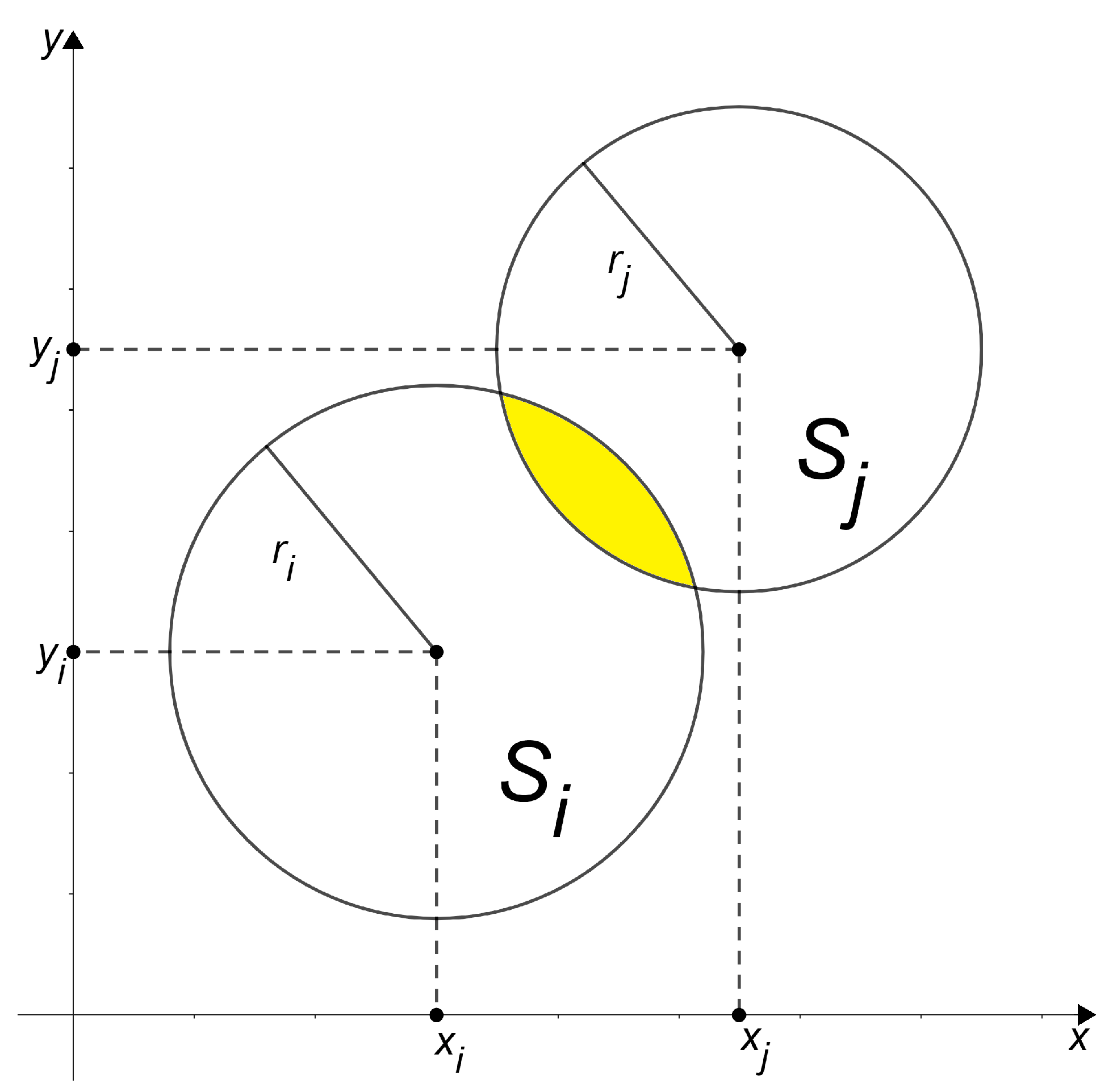
There is a demand zone (region) ${\mathrm{S}}_0$ and a family of service areas ${\mathrm{S}}_1,\dots ,{\mathrm{S}}_{\mathrm{n}}$. Each service area ${\mathrm{S}}_{\mathrm{i}},\mathrm{i}\in {\mathrm{N}}_{\mathrm{n}}$ is associated with a point ${\mathrm{c}}_{\mathrm{i}}$, which we will call a centroid. The areas will be defined relatively to that point. The problem is how to find such a position of service area centroids ${\mathrm{c}}_{\mathrm{i}},\mathrm{i}\in {\mathrm{N}}_{\mathrm{n}}$ in order to provide the optimal service of the demand zone ${\mathrm{S}}_0$ according to a given criterion. It is assumed that the shape and geometric sizes of the demand zone and service areas are specified. Restrictions can be imposed on the position of centroids ${\mathrm{c}}_{\mathrm{i}},\mathrm{i}\in {\mathrm{N}}_{\mathrm{n}}$, which determine their allowable location. As optimality criteria, we will consider the maximum coverage area of the demand zone.

Let us pose this task in terms of the Maximum Coverage Location Problem, considering the demand zone and the service areas as planar geometric items.

2.2. Auxiliary Concepts

In $\mathrm{d}$-dimension Euclidean space ${\mathrm{R}}^{\mathrm{d}}$, an item $\mathrm{S}$ is a geometric set of points $\mathrm{P}\in {\mathrm{R}}^{\mathrm{d}}$ that satisfy an inequality $\mathrm{f}(\mathrm{P})\ge 0$. The equation $\mathrm{f}(\mathrm{P})=0$ defines the boundary of the item $\mathrm{S}$ and its shape. In the general case, the boundary equation contains constants $\mathbf{m}=({\mathrm{m}}_1,\dots ,{\mathrm{m}}_{\mathsf{\alpha }})$, which are called metric parameters, which determines linear sizes of $\mathrm{S}$, i.e., $\mathrm{f}(\mathrm{P},\mathbf{m})=0$. We assume that the function $\mathrm{f}(\mathrm{P},\mathbf{m})$ is defined and continuous in $\mathrm{P}$ for any $\mathbf{m}\in \mathrm{D}$, where $\mathrm{D}$ is the set of admissible values of metric parameters $\mathbf{m}$.

In what follows, we restrict ourselves to a plane problem, so $\mathrm{d}=2$, $\mathrm{P}=(\mathrm{x},\mathrm{y})$.

Consider a fixed Cartesian coordinate system $\mathrm{O}\mathrm{x}\mathrm{y}$. Let us choose a point $\mathrm{c}\in \mathrm{S}$ and associate with the item $\mathrm{S}$ its own (moving) Cartesian coordinate system $\mathrm{O}{\mathrm{x}}^{\prime }{\mathrm{y}}^{\prime }$, with the origin at the point $\mathrm{c}$. The location of the item $\mathrm{S}$ in the coordinate system $\mathrm{O}\mathrm{x}\mathrm{y}$ will be determined by the so-called placement parameters $\mathbf{p}=(\mathbf{v},\mathsf{\theta })$, where $\mathbf{v}=(\mathrm{x},\mathrm{y})$ are the coordinates of the point $\mathrm{c}$ in the fixed coordinate system, and $\mathsf{\theta }$ is the angle of rotation $\mathrm{O}{\mathrm{x}}^{\prime }{\mathrm{y}}^{\prime }$ relative to $\mathrm{O}\mathrm{x}\mathrm{y}$.

The location of an item $\mathrm{S}$ relative to a fixed coordinate system is given by the equation of its general position:

$$\mathrm{F}(\mathrm{P},\mathbf{m},\mathbf{v},\mathsf{\theta })=\mathrm{f}\left(\mathbf{A}(\mathrm{P}\text{-}\mathbf{v}),\mathbf{m}\right)=0,$$

(1)

where the operator $\mathbf{A}$ has the form

$$\mathbf{A}=\left(\begin{array}{r}\cos \mathsf{\theta }\sin \mathsf{\theta }\\ -\sin \mathsf{\theta }\cos \mathsf{\theta }\end{array}\right).$$

Note that the number of placement parameters can be reduced, particularly for centrally symmetrical geometric items. In addition, some placement parameters can be fixed in accordance with the problem statement.

To consider geometric items that have a given shape, but variable metric $\mathbf{m}$ and placement $\mathbf{p}$ parameters, in [28,29] the concept of a configuration space of geometric items $\mathrm{\Xi }(\mathrm{S})$ is introduced, with generalized variables $\mathbf{g}=(\mathbf{m},\mathbf{p})$. Any point $\mathbf{g}=(\mathbf{m},\mathbf{p})$, $\mathbf{m}\in \mathrm{D}$ in this space corresponds to a parametrized geometric item $\mathrm{S}(\mathbf{g})$ such that

$$\begin{array}{c}\mathrm{F}(\mathrm{P},\mathbf{m},\mathbf{p})=0,\mathrm{if}\mathrm{P}\in \mathrm{f}\mathrm{r}\mathrm{S}(\mathbf{g});\\ \mathrm{F}(\mathrm{P},\mathbf{m},\mathbf{p})>0,\mathrm{if}\mathrm{P}\in \mathrm{int}\mathrm{S}(\mathbf{g});\\ \mathrm{F}(\mathrm{P},\mathbf{m},\mathbf{p})<0,\mathrm{if}\mathrm{P}\notin \mathrm{c}\mathrm{l}\mathrm{S}(\mathbf{g}),\end{array}$$

where fr, int, and cl are the operations of the topological boundary, interior, and closure, respectively.

2.3. Math Modeling

Let ${\mathrm{S}}_0$ be a geometric item corresponding to the demand zone and ${\mathrm{S}}_{\mathrm{i}},\mathrm{i}\in {\mathrm{N}}_{\mathrm{n}}^{}$ be a family of geometric items corresponding to the service areas. Analogous with the above definitions, we set the metric and placement parameters ${\mathbf{m}}^{\mathrm{i}}=({\mathrm{m}}_1^{\mathrm{i}},\dots ,{\mathrm{m}}_{{\mathsf{\alpha }}_{\mathrm{i}}}^{\mathrm{i}})$, ${\mathbf{p}}^{\mathrm{i}}=({\mathrm{v}}^{\mathrm{i}},{\mathsf{\theta }}^{\mathrm{i}})$ for ${\mathrm{S}}_{\mathrm{i}},\mathrm{i}\in {\mathrm{N}}_{\mathrm{n}}^0$. Here ${\mathbf{v}}^{\mathrm{i}}=({\mathrm{x}}_{\mathrm{i}},{\mathrm{y}}_{\mathrm{i}})$ are the coordinates of the centroids ${\mathrm{c}}_{\mathrm{i}},\mathrm{i}\in {\mathrm{N}}_{\mathrm{n}}^0$ in the fixed coordinate system $\mathrm{O}\mathrm{x}\mathrm{y}$.

Let us form the configuration spaces $\mathrm{\Xi }({\mathrm{S}}_{\mathrm{i}}),\mathrm{i}\in {\mathrm{N}}_{\mathrm{n}}^0$ of items ${\mathrm{S}}_{\mathrm{i}}$ with generalized variables ${\mathbf{g}}^{\mathrm{i}}=({\mathbf{m}}^{\mathrm{i}},{\mathbf{p}}^{\mathrm{i}})$. Then, we construct the configuration space $\mathrm{\Xi }(\mathrm{\Omega })$ with generalized variables $\mathbf{g}=({\mathbf{g}}^0,{\mathbf{g}}^1,\dots ,{\mathbf{g}}^{\mathrm{n}})$ as a Cartesian product of configuration spaces $\mathrm{\Xi }({\mathrm{S}}_{\mathrm{i}}),\mathrm{i}\in {\mathrm{N}}_{\mathrm{n}}^0$, i.e.,

$$\mathrm{\Xi }(\mathrm{\Omega })=\mathrm{\Xi }({\mathrm{S}}_0)\times \mathrm{\Xi }({\mathrm{S}}_1)\times \dots \times \mathrm{\Xi }({\mathrm{S}}_{\mathrm{n}})$$

Note that depending on the problem statement, some generalized variables may be given. To indicate this, we will use a cap over the corresponding variable.

The solution of the problem posed involves the construction of appropriate mathematical models which are primarily associated with the formalizing of the optimization criterions and constraints, followed by the choice of effective methods for local and global optimization.

In this article, the maximum service coverage of the demand zone is considered as an optimality criterion.

To determine the dependence of the specified optimality criterion on placement parameters ${\mathbf{p}}^{\mathrm{i}},\mathrm{i}\in {\mathrm{N}}_{\mathrm{n}}^{}$ of service areas, an approach based on the concept of a $\mathsf{\omega }$-function [30] for a complex geometric item is proposed.

Let $\mathrm{\Omega }=\left\{{\mathrm{S}}_{\mathrm{i}},\mathrm{i}\in {\mathrm{N}}_{\mathrm{n}}^0\right\}$ be the initial set of geometric items. By the logical operators (union, intersection, difference), we will define a mapping as

$$\mathsf{\phi }:\mathrm{\Omega }\to \mathrm{S}\mathsf{\phi }$$

(2)

that forms a so-called complex item ${\mathrm{S}}_{\mathsf{\phi }}=\mathsf{\phi }({\mathrm{S}}_0,{\mathrm{S}}_1,\dots ,{\mathrm{S}}_{\mathrm{n}})$. We will assume that the mapping $\mathsf{\phi }$ determines the structure of a complex item ${\mathrm{S}}_{\mathsf{\phi }}$.

In the configuration space $\mathrm{\Xi }(\mathrm{\Omega })$, a complex item ${\mathrm{S}}_{\mathsf{\phi }}=\mathsf{\phi }({\mathrm{S}}_0,{\mathrm{S}}_1,\dots ,{\mathrm{S}}_{\mathrm{n}})$ corresponds to a parameterized geometric item

$${\mathrm{S}}_{\mathsf{\phi }}(\mathbf{g})={\mathrm{S}}_{\mathsf{\phi }}({\mathbf{g}}^0,{\mathbf{g}}^1,\dots ,{\mathbf{g}}^{\mathrm{n}})=\mathsf{\phi }\left({\mathrm{S}}_1({\mathbf{g}}^0),{\mathrm{S}}_1({\mathbf{g}}^1),\dots ,{\mathrm{S}}_{\mathrm{n}}({\mathbf{g}}^{\mathrm{n}})\right)$$

Let the sets ${\mathrm{S}}_{\mathrm{i}}({\widehat{\mathbf{g}}}^{\mathrm{i}})\subset {\mathbf{R}}^2,\mathrm{i}\in {\mathrm{N}}_{\mathrm{n}}^0$ be measured by Lebesgue for any ${\widehat{\mathbf{g}}}^{\mathrm{i}}\in \mathrm{\Xi }({\mathrm{S}}_{\mathrm{i}})$. We define a function as

$${\mathsf{\omega }}_{\mathsf{\phi }}(\mathbf{g})={\mathsf{\omega }}_{\mathsf{\phi }}({\mathbf{g}}^0,{\mathbf{g}}^1,\dots ,{\mathbf{g}}^{\mathrm{n}})=\mathsf{\mu }\left({\mathrm{S}}_{\mathsf{\phi }}({\mathbf{g}}^0,{\mathbf{g}}^1,\dots ,{\mathbf{g}}^{\mathrm{n}})\right)$$

where $\mathsf{\mu }(\cdot )$ is the Lebesgue measure.

The function

$${\mathsf{\omega }}_{\mathsf{\phi }}:\mathrm{\Xi }(\mathrm{\Omega })\to {\mathrm{R}}^1$$

defined in this way is called $\mathsf{\omega }$-function [30].

In its essence, for the planar complex parameterized geometric item ${\mathrm{S}}_{\mathsf{\phi }}(\mathbf{g})$, the $\mathsf{\omega }$-function determines the dependence of its area on the generalized variables of the constituent items ${\mathrm{S}}_{\mathrm{i}}({\mathbf{g}}^{\mathrm{i}}),\mathrm{i}\in {\mathrm{N}}_{\mathrm{n}}^0$.

To define the $\mathsf{\omega }$-function, we introduce the characteristic function

$${\mathsf{\lambda }}_{\mathsf{\phi }}(\mathrm{P},\mathbf{g})=\{\begin{array}{l}1,\mathrm{i}\mathrm{f}\mathrm{P}\in {\mathrm{S}}_{\mathsf{\phi }}(\mathbf{g});\\ 0,\mathrm{i}\mathrm{f}\mathrm{P}\notin {\mathrm{S}}_{\mathsf{\phi }}(\mathbf{g}).\end{array}$$

For planar item we have

$${\mathsf{\omega }}_{\mathsf{\phi }}(\mathbf{g})={\displaystyle \iint {\mathsf{\lambda }}_{\mathsf{\phi }}(\mathrm{P},\mathbf{g})\mathrm{d}\mathrm{P}}.$$

(3)

To construct the corresponding $\mathsf{\omega }$-functions, it is necessary to form the configuration spaces of geometric items ${\mathrm{S}}_{\mathrm{i}},\mathrm{i}\in {\mathrm{N}}_{\mathrm{n}}^0$, and write down the equations of their boundaries ${\mathrm{f}}_{\mathrm{i}}(\mathrm{P},{\mathbf{m}}^{\mathrm{i}})=0$ and general positions ${\mathrm{F}}_{\mathrm{i}}(\mathrm{P},{\mathbf{m}}^{\mathrm{i}},{\mathbf{p}}^{\mathrm{i}},{\mathsf{\theta }}^{\mathrm{i}})={\mathrm{f}}_{\mathrm{i}}\left(\mathbf{A}(\mathrm{P}\text{-}{\mathbf{v}}^{\mathrm{i}}),{\mathbf{m}}^{\mathrm{i}}\right)=0$.

In applied problems, geometric items that have the shape of a circle, ellipse, and polygon are most often considered.

For circular items, generalized variables are its radius ${\mathrm{r}}_{\mathrm{i}}$ (metric parameter) and the coordinates of the center $({\mathrm{x}}_{\mathrm{i}},{\mathrm{y}}_{\mathrm{i}})$ in a fixed coordinate system (placement parameters), i.e., ${\mathbf{g}}^{\mathrm{i}}=({\mathbf{m}}^{\mathrm{i}},{\mathbf{p}}^{\mathrm{i}})=({\mathrm{r}}_{\mathrm{i}},{\mathrm{x}}_{\mathrm{i}},{\mathrm{y}}_{\mathrm{i}})$. The general position equation has the form

$${\mathrm{F}}_{\mathrm{i}}(\mathrm{P},{\mathbf{m}}^{\mathrm{i}},{\mathbf{p}}^{\mathrm{i}})={\mathrm{r}}_{\mathrm{i}}^2-{(\mathrm{x}-{\mathrm{x}}_{\mathrm{i}})}^2+{(\mathrm{y}-{\mathrm{y}}_{\mathrm{i}})}^2=0.$$

For an ellipse ${\mathrm{S}}_{\mathrm{i}}$, the generalized variables are semi-major ${\mathrm{a}}_{\mathrm{i}}$ and semi-minor ${\mathrm{b}}_{\mathrm{i}}$ axes, the coordinates $({\mathrm{x}}_{\mathrm{i}},{\mathrm{y}}_{\mathrm{i}})$ of the center of symmetry in a fixed coordinate system, and the angle ${\mathsf{\theta }}_{\mathrm{i}}$ of rotation of its own coordinate system, i.e., ${\mathbf{g}}^{\mathrm{i}}=({\mathbf{m}}^{\mathrm{i}},{\mathbf{p}}^{\mathrm{i}})=({\mathrm{a}}_{\mathrm{i}},{\mathrm{b}}_{\mathrm{i}},{\mathrm{x}}_{\mathrm{i}},{\mathrm{y}}_{\mathrm{i}},{\mathsf{\theta }}_{\mathrm{i}})$. The general position equation can be written as

$${\mathrm{F}}_{\mathrm{i}}(\mathrm{P},{\mathbf{m}}^{\mathrm{i}},{\mathbf{p}}^{\mathrm{i}})=1-\frac{{\left((\mathrm{x}-{\mathrm{x}}_{\mathrm{i}})\cos {\mathsf{\theta }}_{\mathrm{i}}+(\mathrm{y}-{\mathrm{y}}_{\mathrm{i}})\sin {\mathsf{\theta }}_{\mathrm{i}}\right)}^2}{{\mathrm{a}}_{\mathrm{i}}^2}+\frac{{\left((\mathrm{x}-{\mathrm{x}}_{\mathrm{i}})\sin {\mathsf{\theta }}_{\mathrm{i}}-(\mathrm{y}-{\mathrm{y}}_{\mathrm{i}})\cos {\mathsf{\theta }}_{\mathrm{i}}\right)}^2}{{\mathrm{b}}_{\mathrm{i}}^2}=0.$$

For a polygon ${\mathrm{S}}_{\mathrm{i}}$ with ${\mathrm{k}}_{\mathrm{i}}$ vertices, metric parameters can be set, for example, by ordering the coordinates of its vertices in its own coordinate system ${\mathbf{m}}^{\mathrm{i}}=({\widehat{\mathrm{x}}}_1^{\mathrm{i}},{\widehat{\mathrm{y}}}_1^{\mathrm{i}},{\widehat{\mathrm{x}}}_2^{\mathrm{i}},{\widehat{\mathrm{y}}}_2^{\mathrm{i}},\dots ,{\widehat{\mathrm{x}}}_{{\mathrm{k}}_{\mathrm{i}}}^{\mathrm{i}},{\widehat{\mathrm{y}}}_{{\mathrm{k}}_{\mathrm{i}}}^{\mathrm{i}})$. The placement parameters will be the coordinates of the system origin $({\mathrm{x}}_{\mathrm{i}},{\mathrm{y}}_{\mathrm{i}})$ and the angle ${\mathsf{\theta }}_{\mathrm{i}}$ of its rotation, i.e., ${\mathbf{g}}^{\mathrm{i}}=({\mathbf{m}}^{\mathrm{i}},{\mathbf{p}}^{\mathrm{i}})=({\widehat{\mathrm{x}}}_1^{\mathrm{i}},{\widehat{\mathrm{y}}}_1^{\mathrm{i}},{\widehat{\mathrm{x}}}_2^{\mathrm{i}},{\widehat{\mathrm{y}}}_2^{\mathrm{i}},\dots ,{\widehat{\mathrm{x}}}_{{\mathrm{k}}_{\mathrm{i}}}^{\mathrm{i}},{\widehat{\mathrm{y}}}_{{\mathrm{k}}_{\mathrm{i}}}^{\mathrm{i}},{\mathrm{x}}_{\mathrm{i}},{\mathrm{y}}_{\mathrm{i}},{\mathsf{\theta }}_{\mathrm{i}})$. The general position equation ${\mathrm{F}}_{\mathrm{i}}(\mathrm{P},{\mathbf{m}}^{\mathrm{i}},{\mathbf{p}}^{\mathrm{i}})=0$ is easy to write using the equations of lines passing through adjacent vertices of the polygon.

To use the approach described above to solve the problem posed in this article, we consider the formation of complex items based on mapping (2). Let us put the family of mappings as

$$\mathsf{\psi }:\mathrm{\Omega }\to \mathrm{S}\mathsf{\psi }$$

(4)

$${\mathsf{\psi }}_{\mathrm{i}\mathrm{j}}:\mathrm{\Omega }\to \mathrm{S}{\mathsf{\psi }}_{\mathrm{i}\mathrm{j}},\mathrm{i},\mathrm{j}\in {\mathrm{N}}_{\mathrm{n}}^0,\mathrm{j}>\mathrm{i},$$

(5)

where

$${\mathrm{S}}_{\mathsf{\psi }}=\mathsf{\psi }({\mathrm{S}}_0,{\mathrm{S}}_1,\dots ,{\mathrm{S}}_{\mathrm{n}})={\mathrm{S}}_0\cap {\displaystyle \underset{\mathrm{i}=1}{\overset{\mathrm{n}}{\cup }}{\mathrm{S}}_{\mathrm{i}}}$$

(6)

$$\mathrm{S}{\mathsf{\psi }}_{\mathrm{i}\mathrm{j}}={\mathsf{\psi }}_{\mathrm{i}\mathrm{j}}({\mathrm{S}}_0,{\mathrm{S}}_1,\dots ,{\mathrm{S}}_{\mathrm{n}})={\mathrm{S}}_{\mathrm{i}}\cap {\mathrm{S}}_{\mathrm{j}},\mathrm{i},\mathrm{j}\in {\mathrm{N}}_{\mathrm{n}}^0,\mathrm{j}>\mathrm{i}.$$

We fix the location of the demand zone by setting ${\widehat{\mathbf{p}}}^0=(0,0,0)$ and setting the metric parameters ${\widehat{\mathbf{m}}}^{\mathrm{i}},\mathrm{i}\in {\mathrm{N}}_{\mathrm{n}}^0$ of the demand zone and service areas. Then,

$${\mathbf{g}}^0=({\widehat{\mathbf{m}}}^0,{\mathbf{p}}^0),{\mathbf{g}}^{\mathrm{i}}=({\widehat{\mathbf{m}}}^{\mathrm{i}},{\mathbf{p}}^{\mathrm{i}}),\mathrm{i}\in {\mathrm{N}}_{\mathrm{n}}^{}.$$

Considering that both metric parameters ${\widehat{\mathbf{m}}}^{\mathrm{i}},\mathrm{i}\in {\mathrm{N}}_{\mathrm{n}}^0$ and the placement parameters ${\widehat{\mathbf{p}}}^0$ are given, our goal is to find the placement parameters ${\mathbf{p}}^{\mathrm{i}},\mathrm{i}\in {\mathrm{N}}_{\mathrm{n}}^{}$ of service areas that provide the maximum service coverage. Note that with the given metric parameters ${\widehat{\mathbf{m}}}^{\mathrm{i}},\mathrm{i}\in {\mathrm{N}}_{\mathrm{n}}^0$ of geometric objects, their Lebesgue measure (area) does not depend on placement parameters, i.e., ${\mathsf{\mu }}_{\mathrm{i}}=\mathsf{\mu }({\mathrm{S}}_{\mathrm{i}})$.

The dependence of the coverage area of the demand zone ${\mathrm{S}}_0$ on placement parameters ${\mathbf{p}}^{\mathrm{i}}=({\mathrm{x}}_{\mathrm{i}},{\mathrm{y}}_{\mathrm{i}},{\mathsf{\theta }}_{\mathrm{i}})$ of service areas ${\mathrm{S}}_{\mathrm{i}},\mathrm{i}\in {\mathrm{N}}_{\mathrm{n}}^{}$ can be represented as

$$\mathrm{W}({\mathbf{p}}^1,\dots ,{\mathbf{p}}^{\mathrm{n}})={\mathsf{\omega }}_{\mathsf{\psi }}(\mathbf{g})={\mathsf{\omega }}_{\mathsf{\psi }}({\widehat{\mathbf{m}}}^0,{\widehat{\mathbf{p}}}^0,{\widehat{\mathbf{m}}}^1,{\mathbf{p}}^1,\dots ,{\widehat{\mathbf{m}}}^{\mathrm{n}},{\mathbf{p}}^{\mathrm{n}}),$$

where the mapping $\mathsf{\psi }$ has the form (4).

As a result, we have a nonlinear optimization problem

$$\mathrm{W}({\mathbf{p}}^1,\dots ,{\mathbf{p}}^{\mathrm{n}})\to \max$$

(7)

subject to

$$({\mathbf{p}}^1,\dots ,{\mathbf{p}}^{\mathrm{n}})\in \mathrm{D},$$

where $\mathrm{D}$ is a feasible region, which is given by restrictions on the location of centroids

$${\mathrm{c}}_{\mathrm{i}},\mathrm{i}\in {\mathrm{N}}_{\mathrm{n}}.$$

An example of such restrictions can be the conditions for the minimum ${\mathrm{d}}_{\mathrm{i}\mathrm{j}}^{\min }$ and maximum ${\mathrm{d}}_{\mathrm{i}\mathrm{j}}^{\max }$ distances between centroids ${\mathrm{c}}_{\mathrm{i}}$ and ${\mathrm{c}}_{\mathrm{j}}$, $\mathrm{i},\mathrm{j}\in {\mathrm{N}}_{\mathrm{n}},\mathrm{j}>\mathrm{i}$ which have the form

$${\mathrm{d}}_{\mathrm{i}\mathrm{j}}^{\min }\le \sqrt{{({\mathrm{x}}_{\mathrm{i}}-{\mathrm{x}}_{\mathrm{j}})}^2+{({\mathrm{y}}_{\mathrm{i}}-{\mathrm{y}}_{\mathrm{j}})}^2}\le {\mathrm{d}}_{\mathrm{i}\mathrm{j}}^{\max }.$$

2.4. Decision Optimization Using Computer Geometry Software

The optimization problem (7) is high-dimensional and multi-extremal. The ways to solve it are determined by the properties of the function $\mathrm{W}({\mathbf{p}}^1,\dots ,{\mathbf{p}}^{\mathrm{n}})$. Unfortunately, it is impossible to obtain an analytical expression for $\mathrm{W}({\mathbf{p}}^1,\dots ,{\mathbf{p}}^{\mathrm{n}})$ in the form of a dependence on variables ${\mathbf{p}}^{\mathrm{i}}=({\mathrm{x}}_{\mathrm{i}},{\mathrm{y}}_{\mathrm{i}},{\mathsf{\theta }}_{\mathrm{i}})$, $\mathrm{i}\in {\mathrm{N}}_{\mathrm{n}}^{}$. Indeed, for this it is necessary to carry out integration according to formula (3), which is an impossible task for regions of a complex shape. We propose to calculate the function $\mathrm{W}({\mathbf{p}}^1,\dots ,{\mathbf{p}}^{\mathrm{n}})$ using modern computational geometry packages. The features of the implementation of such packages when solving placement and coverage problems using $\mathsf{\omega }$-functions are described in [31,32,33].

Currently, you can find a wide list of libraries that allow you to operate with complex geometric shapes, in particular, SymPy, Shapely, CGAL, SpaceFuncs, and many others. Based on the analysis of these libraries, taking into account the necessary functionality for calculating the function $\mathrm{W}({\mathbf{p}}^1,\dots ,{\mathbf{p}}^{\mathrm{n}})$, we chose the Shapely library [34] of the Python algorithmic language.

Shapely is created for the theoretical analysis of point sets and the manipulation of planar objects using the functions of the GEOS library through the ctypes Python module. GEOS as a port of the Java Topology Suite package is the geometry attribute of the spatial extension of PostGIS. At the same time, Shapely adheres mainly to uniform standard classes and operations.

The Shapely library makes it possible to perform operations on geometric shapes using logical operators (union, intersection, difference, and complement) and to build complex shapes on the plane from a set of basic shapes (polygon, circle, and ellipse). To model basic shapes, the geometry module is used, which includes the Point and Polygon classes. We import the Point and Polygon classes for geometry items from Shapely as follows:

from shapely.geometry.point import Point

from shapely.geometry import Polygon

A point is given by its coordinates and a polygon by an array of vertex coordinates. When using the Shapely library, the complexity of the shape does not matter and only affects the calculation time. At the same time, geometric items are created typically for Python through the instance factory. If necessary, factories can be checked for topological simplicity or validity using the predicate: attr:is_valid.

Since there is no special data type for circle and ellipse in the Shapely library, the affinity module is used to construct them. A set of affine transformation functions is contained in the shapely.affinity module, which returns geometric shapes by directly providing coefficients to the affine transformation matrix or by using a custom named transformation (rotate, scale, etc.).

To build a circle, you need a standard set of its generalized parameters—the coordinates of the center (x, y) and the radius r:

circle_center = Point(x, y)

circle = circle_center.buffer(r)

For an ellipse, the major semi-axis a and the minor semi-axis b are used:

ellipse_center = Point(x, y).buffer(1)

ellipse = affinity.scale(ellipse_center, a, b),

where the affinity.scale function scales the item according to the values of the semi-axes.

The function affinity.rotate (item, $\theta$) is used to rotate the item by an angle $\theta$. Here ‘item’ specifies the shape (polygon, ellipse, or complex shape). However, in any case, as a result of the affine transformation, an item belonging to the Polygon class is built. This is the main reason for the simplicity of operations between the complex items, since, in fact, these are operations on polygons. Logical operations difference, intersection, union, symmetric_difference are used for any two items in the geometry module.

From the point of view of using the Shapely library, the ability to calculate the area of a complex geometric item is fundamental. There is an area field for this. When forming any item, its area is calculated automatically.

The ability to calculate the function $\mathrm{W}({\widehat{\mathbf{p}}}^1,\dots ,{\widehat{\mathbf{p}}}^{\mathrm{n}})$ for any fixed placement parameters $({\widehat{\mathbf{p}}}^1,\dots ,{\widehat{\mathbf{p}}}^{\mathrm{n}})$ allows the use of modern methods of local and global optimization to solve problem (7). However, this requires too much computation of this function. Therefore, there is a question around the development of effective approaches that reduce their computational complexity.

Based on the specifics of the problem statement, we offer the following approach. Let us consider the auxiliary optimization problem, which consists in minimizing the total area of paired overlaps of service areas and their overlap with the complement of the demand zone.

The auxiliary problem is formulated as

$$\mathrm{G}({\mathbf{p}}^1,\dots ,{\mathbf{p}}^{\mathrm{n}})\to \min ,$$

(8)

where

$$\mathrm{G}({\mathbf{p}}^1,\dots ,{\mathbf{p}}^{\mathrm{n}})={\displaystyle \sum _{\mathrm{i}=1}^{\mathrm{n}-1}{\displaystyle \sum _{\mathrm{j}=\mathrm{i}+1}^{\mathrm{n}}{\mathsf{\omega }}_{{\mathsf{\psi }}_{\mathrm{i}\mathrm{j}}}}}({\mathbf{g}}^{\mathrm{i}},{\mathbf{g}}^{\mathrm{j}})-{\displaystyle \sum _{\mathrm{j}=1}^{\mathrm{n}}{\mathsf{\omega }}_{{\mathsf{\psi }}_{0\mathrm{j}}}({\widehat{\mathbf{g}}}^0,{\mathbf{g}}^{\mathrm{j}})}+{\displaystyle \sum _{\mathrm{j}=1}^{\mathrm{n}}{\mathsf{\mu }}_{\mathrm{j}}};$$

(9)

the family of mappings ${\mathsf{\psi }}_{\mathrm{i}\mathrm{j}}$, $\mathrm{i},\mathrm{j}\in {\mathrm{N}}_{\mathrm{n}}^0$, $\mathrm{j}>\mathrm{i}$ have the form (4);

${\mathsf{\mu }}_{\mathrm{j}}$, $\mathrm{j}\in {\mathrm{N}}_{\mathrm{n}}^{}$ are constants equal to the item areas ${\mathrm{S}}_{\mathrm{i}},\mathrm{i}\in {\mathrm{N}}_{\mathrm{n}}^{}$.

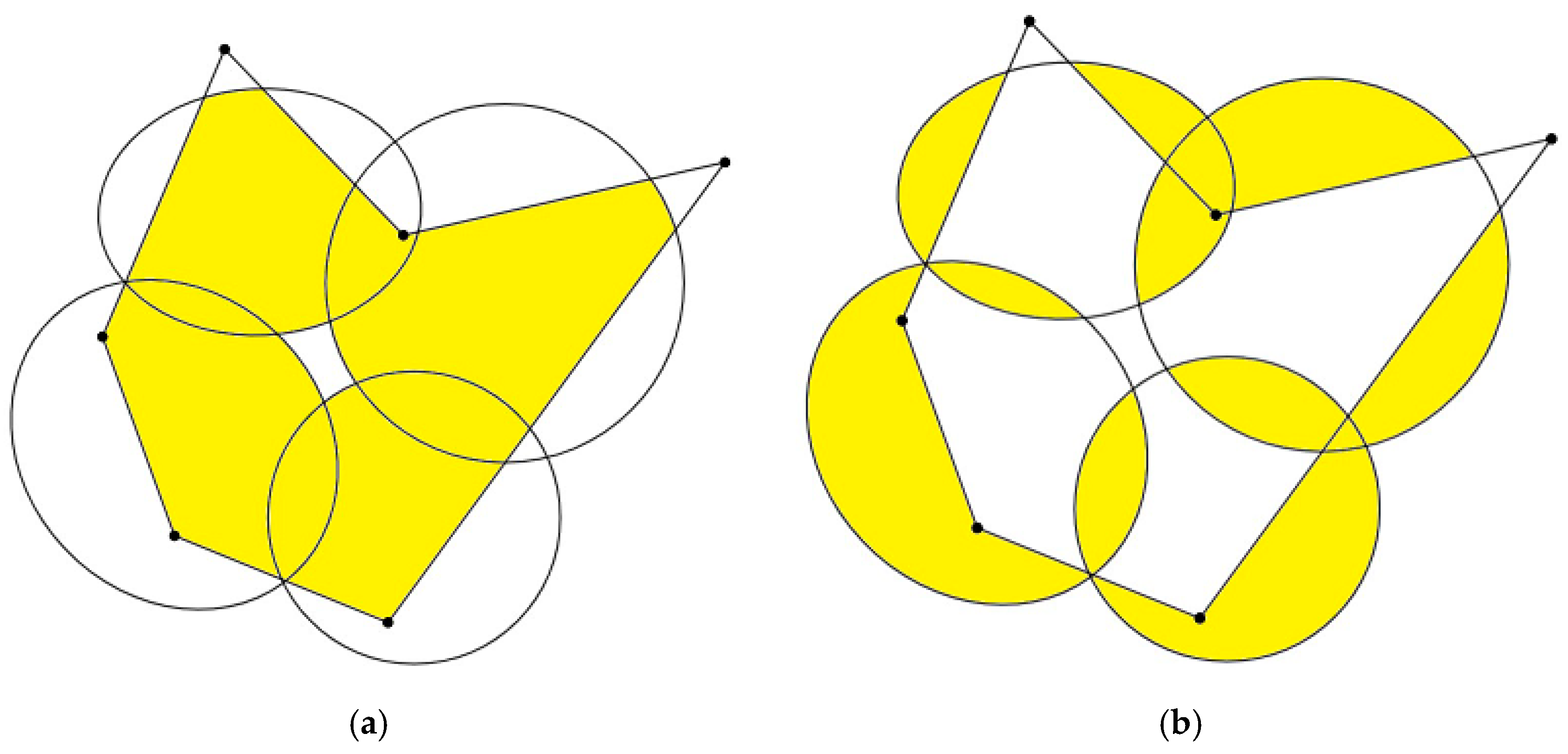
To clarify the geometric meaning of the functions $\mathrm{W}({\widehat{\mathbf{p}}}^1,\dots ,{\widehat{\mathbf{p}}}^{\mathrm{n}})$ and $\mathrm{G}({\widehat{\mathbf{p}}}^1,\dots ,{\widehat{\mathbf{p}}}^{\mathrm{n}})$ for the fixed placement parameters of items, we present Figure 1. In Figure 1a, the service coverage is shown. In Figure 1b, the overlapping of service areas between themselves and with the demand zone complement are also colored.

Obviously, it is expected that the solution to problem (8) will be a good approximation for problem (7). This assumption is confirmed by the test tasks presented in the next section.

The main advantage of problem (8) is that in order to calculate functions ${\mathsf{\omega }}_{{\mathsf{\psi }}_{0\mathrm{j}}}({\widehat{\mathbf{g}}}^0,{\mathbf{g}}^{\mathrm{j}})$, ${\mathsf{\omega }}_{{\mathsf{\psi }}_{\mathrm{i}\mathrm{j}}}({\mathbf{g}}^{\mathrm{i}},{\mathbf{g}}^{\mathrm{j}})$, $\mathrm{i},\mathrm{j}\in {\mathrm{N}}_{\mathrm{n}}^{}$, $\mathrm{j}>\mathrm{i}$, using the Shapely library, there is no need to form a complex item (6), but it is enough to consider only the operations of the intersection of two items. Moreover, for geometric items of a simple shape (circles, ellipses, and polygons), formulas are known for the dependence of the intersection area of items on their placement parameters.

Based on the above reasoning, we propose the following approach to solving problem (7), highlighting the stages of local and global optimization. At the stage of local optimization for the starting point $({\widehat{\mathbf{p}}}^1,\dots ,{\widehat{\mathbf{p}}}^{\mathrm{n}})$, we find the local minimum $({\tilde{\mathbf{p}}}^1,\dots ,{\tilde{\mathbf{p}}}^{\mathrm{n}})$ of the function $\mathrm{G}({\mathbf{p}}^1,\dots ,{\mathbf{p}}^{\mathrm{n}})$. To solve this problem, the Nelder–Mead method or an efficient gradient method can be used. If analytical expressions for the functions ${\mathsf{\omega }}_{{\mathsf{\psi }}_{0\mathrm{j}}}({\widehat{\mathbf{g}}}^0,{\mathbf{g}}^{\mathrm{j}})$, ${\mathsf{\omega }}_{{\mathsf{\psi }}_{\mathrm{i}\mathrm{j}}}({\mathbf{g}}^{\mathrm{i}},{\mathbf{g}}^{\mathrm{j}})$, $\mathrm{i},\mathrm{j}\in {\mathrm{N}}_{\mathrm{n}}^{}$, $\mathrm{j}>\mathrm{i}$ are known, then the calculation of their gradients does not cause difficulties. In general, first order differences can be used. Then the value of the function $\mathrm{W}({\tilde{\mathbf{p}}}^1,\dots ,{\tilde{\mathbf{p}}}^{\mathrm{n}})$ is found, and the point $({\tilde{\mathbf{p}}}^1,\dots ,{\tilde{\mathbf{p}}}^{\mathrm{n}})$ is considered as an approximation to the local solution of the problem (7). Note that for the function ${\mathsf{\omega }}_{\mathsf{\psi }}({\widehat{\mathbf{m}}}^0,{\widehat{\mathbf{p}}}^0,{\widehat{\mathbf{m}}}^1,{\mathbf{p}}^1,\dots ,{\widehat{\mathbf{m}}}^{\mathrm{n}},{\mathbf{p}}^{\mathrm{n}})$, the calculation of the first order differences has features that are studied in [33].

At the stage of the global optimization, a multi-start method was used, when at each iteration, initial points $({\widehat{\mathbf{p}}}^1,\dots ,{\widehat{\mathbf{p}}}^{\mathrm{n}})$ were randomly generated, approximations to the local minimum $({\tilde{\mathbf{p}}}^1,\dots ,{\tilde{\mathbf{p}}}^{\mathrm{n}})$ of the function were found $\mathrm{G}({\mathbf{p}}^1,\dots ,{\mathbf{p}}^{\mathrm{n}})$, and values $\mathrm{W}({\tilde{\mathbf{p}}}^1,\dots ,{\tilde{\mathbf{p}}}^{\mathrm{n}})$ were calculated. After all iterations, the best point $({\tilde{\mathbf{p}}}^1,\dots ,{\tilde{\mathbf{p}}}^{\mathrm{n}})$ was chosen as the starting point for local optimization of the function $\mathrm{W}({\mathbf{p}}^1,\dots ,{\mathbf{p}}^{\mathrm{n}})$. The resulting solution is considered as a solution to problem (7).

3. Results

We implemented the approach described above to solve the following problem. Let the demand zone ${\mathrm{S}}_0$ be a polygon, and the service areas ${\mathrm{S}}_{\mathrm{i}},\mathrm{i}\in {\mathrm{N}}_{\mathrm{n}}^{}$ have a circular shape with generalized variables ${\mathbf{g}}^{\mathrm{i}}=({\widehat{\mathbf{m}}}^{\mathrm{i}},{\mathbf{p}}^{\mathrm{i}})=({\mathrm{r}}_{\mathrm{i}},{\mathrm{x}}_{\mathrm{i}},{\mathrm{y}}_{\mathrm{i}})$, where ${\mathrm{r}}_{\mathrm{i}}$ is the given radius; $({\mathrm{x}}_{\mathrm{i}},{\mathrm{y}}_{\mathrm{i}})$ are the coordinates of the circle center in the fixed coordinate system $\mathrm{O}\mathrm{x}\mathrm{y}$ (Figure 2).

The following formulas were used to calculate the functions ${\mathsf{\omega }}_{{\mathsf{\psi }}_{\mathrm{i}\mathrm{j}}}({\mathbf{g}}^{\mathrm{i}},{\mathbf{g}}^{\mathrm{j}})$, $\mathrm{i},\mathrm{j}\in {\mathrm{N}}_{\mathrm{n}}^{}$, $\mathrm{j}>\mathrm{i}$ and their gradients:

$${\mathsf{\omega }}_{{\mathsf{\psi }}_{\mathrm{i}\mathrm{j}}}({\mathbf{g}}^{\mathrm{i}},{\mathbf{g}}^{\mathrm{j}})={\mathrm{r}}_{\mathrm{i}}^2\mathrm{c}\mathrm{o}{\mathrm{s}}^{-1}\frac{{}_{{\mathrm{r}}_{\mathrm{i}}^2-{\mathrm{r}}_{\mathrm{j}}^2+{({\mathrm{x}}_{\mathrm{i}}-{\mathrm{x}}_{\mathrm{j}})}^2+{({\mathrm{y}}_{\mathrm{i}}-{\mathrm{y}}_{\mathrm{j}})}^2}}{2{\mathrm{r}}_{\mathrm{i}}^{}\sqrt{{({\mathrm{x}}_{\mathrm{i}}-{\mathrm{x}}_{\mathrm{j}})}^2+{({\mathrm{y}}_{\mathrm{i}}-{\mathrm{y}}_{\mathrm{j}})}^2}}-$$

$$-\frac{{\mathrm{r}}_{\mathrm{i}}^2-{\mathrm{r}}_{\mathrm{j}}^2+{({\mathrm{x}}_{\mathrm{i}}-{\mathrm{x}}_{\mathrm{j}})}^2+{({\mathrm{y}}_{\mathrm{i}}-{\mathrm{y}}_{\mathrm{j}})}^2}{2\sqrt{{({\mathrm{x}}_{\mathrm{i}}-{\mathrm{x}}_{\mathrm{j}})}^2+{({\mathrm{y}}_{\mathrm{i}}-{\mathrm{y}}_{\mathrm{j}})}^2}}\sqrt{{\mathrm{r}}_{\mathrm{i}}^2-\frac{{{}_{\left({\mathrm{r}}_{\mathrm{i}}^2-{\mathrm{r}}_{\mathrm{j}}^2+{({\mathrm{x}}_{\mathrm{i}}-{\mathrm{x}}_{\mathrm{j}})}^2+{({\mathrm{y}}_{\mathrm{i}}-{\mathrm{y}}_{\mathrm{j}})}^2\right)}}^2}{4\left({({\mathrm{x}}_{\mathrm{i}}-{\mathrm{x}}_{\mathrm{j}})}^2+{({\mathrm{y}}_{\mathrm{i}}-{\mathrm{y}}_{\mathrm{j}})}^2\right)}}+$$

$$+{\mathrm{r}}_{\mathrm{j}}^2\mathrm{c}\mathrm{o}{\mathrm{s}}^{-1}\frac{{}_{{\mathrm{r}}_{\mathrm{j}}^2-{\mathrm{r}}_{\mathrm{i}}^2+{({\mathrm{x}}_{\mathrm{i}}-{\mathrm{x}}_{\mathrm{j}})}^2+{({\mathrm{y}}_{\mathrm{i}}-{\mathrm{y}}_{\mathrm{j}})}^2}}{2{\mathrm{r}}_{\mathrm{j}}^{}\sqrt{{({\mathrm{x}}_{\mathrm{i}}-{\mathrm{x}}_{\mathrm{j}})}^2+{({\mathrm{y}}_{\mathrm{i}}-{\mathrm{y}}_{\mathrm{j}})}^2}}-$$

$$-\frac{{\mathrm{r}}_{\mathrm{j}}^2-{\mathrm{r}}_{\mathrm{i}}^2+{({\mathrm{x}}_{\mathrm{i}}-{\mathrm{x}}_{\mathrm{j}})}^2+{({\mathrm{y}}_{\mathrm{i}}-{\mathrm{y}}_{\mathrm{j}})}^2}{2\sqrt{{({\mathrm{x}}_{\mathrm{i}}-{\mathrm{x}}_{\mathrm{j}})}^2+{({\mathrm{y}}_{\mathrm{i}}-{\mathrm{y}}_{\mathrm{j}})}^2}}\sqrt{{\mathrm{r}}_{\mathrm{j}}^2-\frac{{{}_{\left({\mathrm{r}}_{\mathrm{j}}^2-{\mathrm{r}}_{\mathrm{i}}^2+{({\mathrm{x}}_{\mathrm{i}}-{\mathrm{x}}_{\mathrm{j}})}^2+{({\mathrm{y}}_{\mathrm{i}}-{\mathrm{y}}_{\mathrm{j}})}^2\right)}}^2}{4\left({({\mathrm{x}}_{\mathrm{i}}-{\mathrm{x}}_{\mathrm{j}})}^2+{({\mathrm{y}}_{\mathrm{i}}-{\mathrm{y}}_{\mathrm{j}})}^2\right)}}$$

(10)

The functions ${\mathsf{\omega }}_{{\mathsf{\psi }}_{0\mathrm{j}}}({\widehat{\mathbf{g}}}^0,{\widehat{\mathbf{g}}}^{\mathrm{j}})$, $\mathrm{j}\in {\mathrm{N}}_{\mathrm{n}}^{}$ were calculated algorithmically using the Shapely library. Polygon ${\mathrm{S}}_0$ generalized variables ${\widehat{\mathbf{g}}}^0=({\widehat{\mathbf{m}}}^0,{\mathbf{p}}^0)$ were specified by a list of vertex coordinates (vert_coords) and ${\mathbf{p}}^0=(0,0,0)$. The Python code instance is as follows:

from shapely.geometry.point import Point

from shapely.geometry import Polygon

region = Polygon(region_vert_coord)

circle = [Point(center_coord[i]).buffer(r[i]) for i in range(n)]

result_functionG = 0

for i in range(n):

 result_functionG += region.intersection(circle[i]).area

To find the local minimum of the function $\mathrm{G}({\mathbf{p}}^1,\dots ,{\mathbf{p}}^{\mathrm{n}})$ given by formula (9), we used the Broyden–Fletcher–Goldfarb–Shanno (BFGS) method [35]. The gradients of the functions ${\mathsf{\omega }}_{{\mathsf{\psi }}_{\mathrm{i}\mathrm{j}}}({\mathbf{g}}^{\mathrm{i}},{\mathbf{g}}^{\mathrm{j}})$, $\mathrm{i},\mathrm{j}\in {\mathrm{N}}_{\mathrm{n}}^{}$, $\mathrm{j}>\mathrm{i}$ were calculated analytically based on formula (10), and for the functions ${\mathsf{\omega }}_{{\mathsf{\psi }}_{0\mathrm{j}}}({\widehat{\mathbf{g}}}^0,{\widehat{\mathbf{g}}}^{\mathrm{j}})$, $\mathrm{j}\in {\mathrm{N}}_{\mathrm{n}}^{}$, first order differences were used.

To find the local maximum of the function $\mathrm{W}({\mathbf{p}}^1,\dots ,{\mathbf{p}}^{\mathrm{n}})$, we also used the BFGS method with first-order differences. In this case, the function ${\mathsf{\omega }}_{\mathsf{\psi }}({\widehat{\mathbf{m}}}^0,{\widehat{\mathbf{p}}}^0,{\widehat{\mathbf{m}}}^1,{\mathbf{p}}^1,\dots ,{\widehat{\mathbf{m}}}^{\mathrm{n}},{\mathbf{p}}^{\mathrm{n}})$ was calculated algorithmically using the Shapely library according to the Python code instance

circle_loc = [Point(center_coord_loc[i]).buffer(r[i]) for i in range(n)]

result_areaW = region.intersection(unary_union(circle_loc)).area

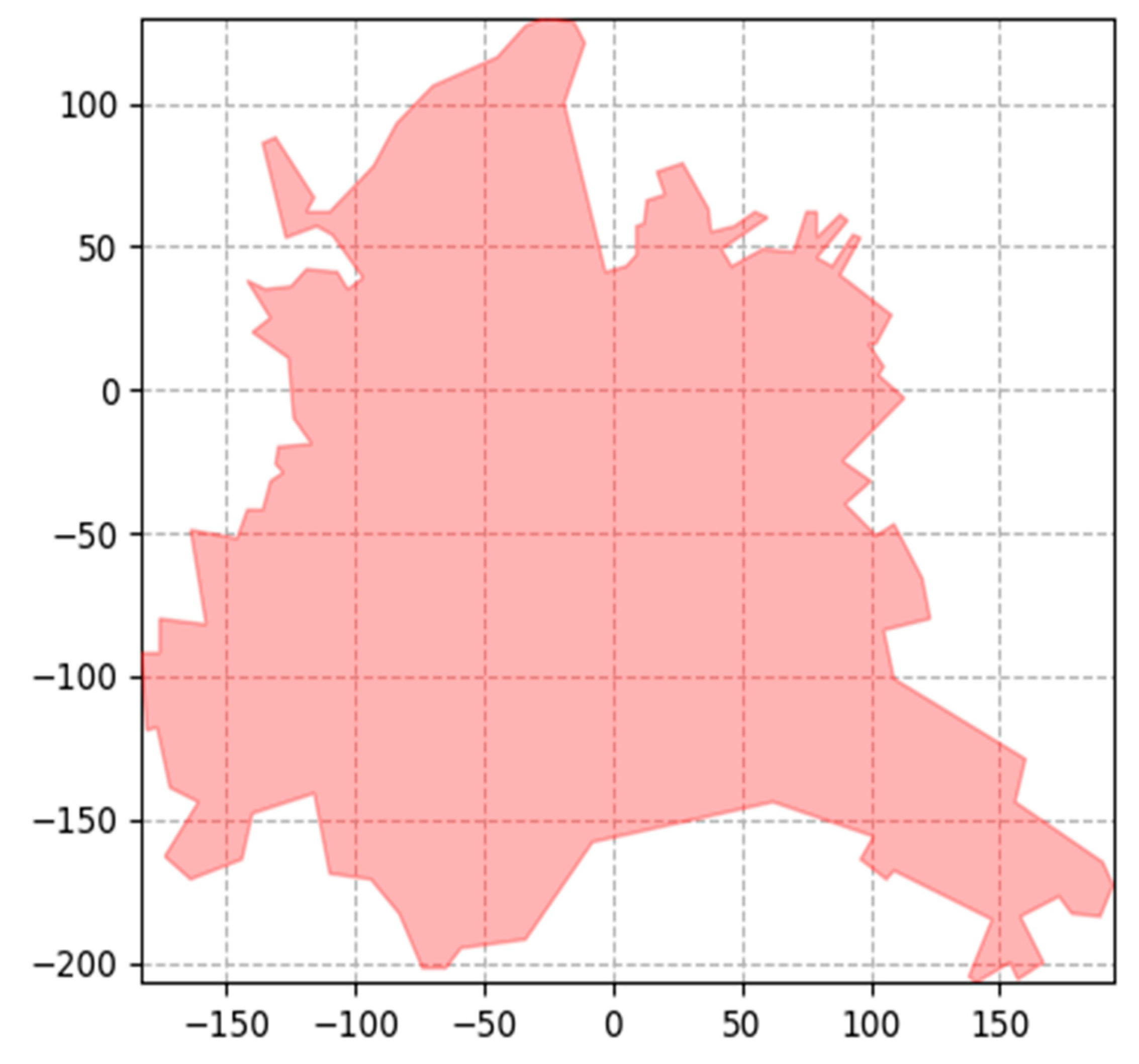
For the numerical implementation of the approach, we chose the polygon ${\mathrm{S}}_0$ corresponding to the Kharkiv region (Ukraine) as the demand zone. Figure 3 shows this region, and

Table 1. Coordinates of the polygon vertices of the demand zone.

$\mathbf{i}$	${\mathbf{x}}_{\mathbf{i}}$	${\mathbf{y}}_{\mathbf{i}}$	$\mathbf{i}$	${\mathbf{x}}_{\mathbf{i}}$	${\mathbf{y}}_{\mathbf{i}}$	$\mathbf{i}$	${\mathbf{x}}_{\mathbf{i}}$	${\mathbf{y}}_{\mathbf{i}}$	$\mathbf{i}$	${\mathbf{x}}_{\mathbf{i}}$	${\mathbf{y}}_{\mathbf{i}}$	$\mathbf{i}$	${\mathbf{x}}_{\mathbf{i}}$	${\mathbf{y}}_{\mathbf{i}}$
1	−174	−163	25	−125	36	49	9	47	73	96	53	97	158	−184
2	−161	−144	26	−119	42	50	9	57	74	88	40	98	167	−200
3	−172	−139	27	−107	41	51	12	58	75	108	26	99	157	−206
4	−177	−118	28	−103	35	52	13	66	76	102	16	100	154	−200
5	−181	−119	29	−97	39	53	20	68	77	99	16	101	141	−207
6	−183	−92	30	−109	54	54	17	76	78	105	8	102	138	−205
7	−176	−92	31	−115	57	55	27	79	79	103	5	103	147	−185
8	−176	−80	32	−127	53	56	37	63	80	113	−3	104	109	−168
9	−158	−82	33	−136	86	57	38	55	81	89	−25	105	106	−171
10	−164	−49	34	−131	88	58	47	57	82	100	−32	106	96	−164
11	−146	−52	35	−116	67	59	55	62	83	90	−40	107	101	−156
12	−142	−42	36	−119	62	60	60	60	84	102	−51	108	62	−144
13	−136	−42	37	−110	62	61	42	49	85	109	−47	109	−8	−158
14	−133	−32	38	−93	78	62	46	43	86	120	−66	110	−34	−192
15	−128	−29	39	−84	93	63	58	49	87	123	−80	111	−59	−195
16	−131	−26	40	−70	106	64	70	48	88	105	−84	112	−65	−202
17	−130	−20	41	−45	116	65	75	62	89	109	−101	113	−74	−202
18	−117	−19	42	−34	127	66	79	62	90	160	−129	114	−83	−183
19	−124	−10	43	−26	130	67	79	53	91	156	−144	115	−94	−171
20	−126	11	44	−15	128	68	88	61	92	190	−165	116	−110	−169
21	−140	20	45	−11	121	69	91	59	93	194	−173	117	−116	−141
22	−133	25	46	−19	100	70	79	46	94	189	−184	118	−140	−148
23	−142	38	47	−3	41	71	85	43	95	178	−183	119	−144	−164
24	−135	35	48	5	43	72	93	54	96	173	−177	120	−164	−171

lists the coordinates of the vertices of ${\mathrm{S}}_0$. As service areas, the 30 circles ${\mathrm{S}}_{\mathrm{i}},\mathrm{i}\in {\mathrm{N}}_{30}^{}$ are considered and the radii ${\mathrm{r}}_{\mathrm{i}},\mathrm{i}\in {\mathrm{N}}_{30}^{}$, both of which are presented in

Table 2. Radii of circular service areas.

i	ri	i	ri	i	ri	i	ri	i	ri
1	16.4	7	20.4	13	24.4	19	28.4	25	32.4
2	17.1	8	21.1	14	25.1	20	29.1	26	33.1
3	17.8	9	21.8	15	25.8	21	29.8	27	33.8
4	18.4	10	22.4	16	26.4	22	30.4	28	34.4
5	19.1	11	23.1	17	27.1	23	31.1	29	35.1
6	19.8	12	23.8	18	27.8	24	31.8	30	35.8

. The polygon ${\mathrm{S}}_0$ area is 65,837 units, the total area of the 30 circles is 67,343.5 units.

We used a computer with the following configuration: Intel Core i7-5557U processor, CPU Speed 3.1 GHz, 2 cores, 4 threads; RAM 16 GB DDR3 1866 MHz; Graphics processor Intel Iris Graphics 6100 with 1.5 GB of video memory; SSD 512 GB; Operating system Mac OS X11.0 Big Sur.

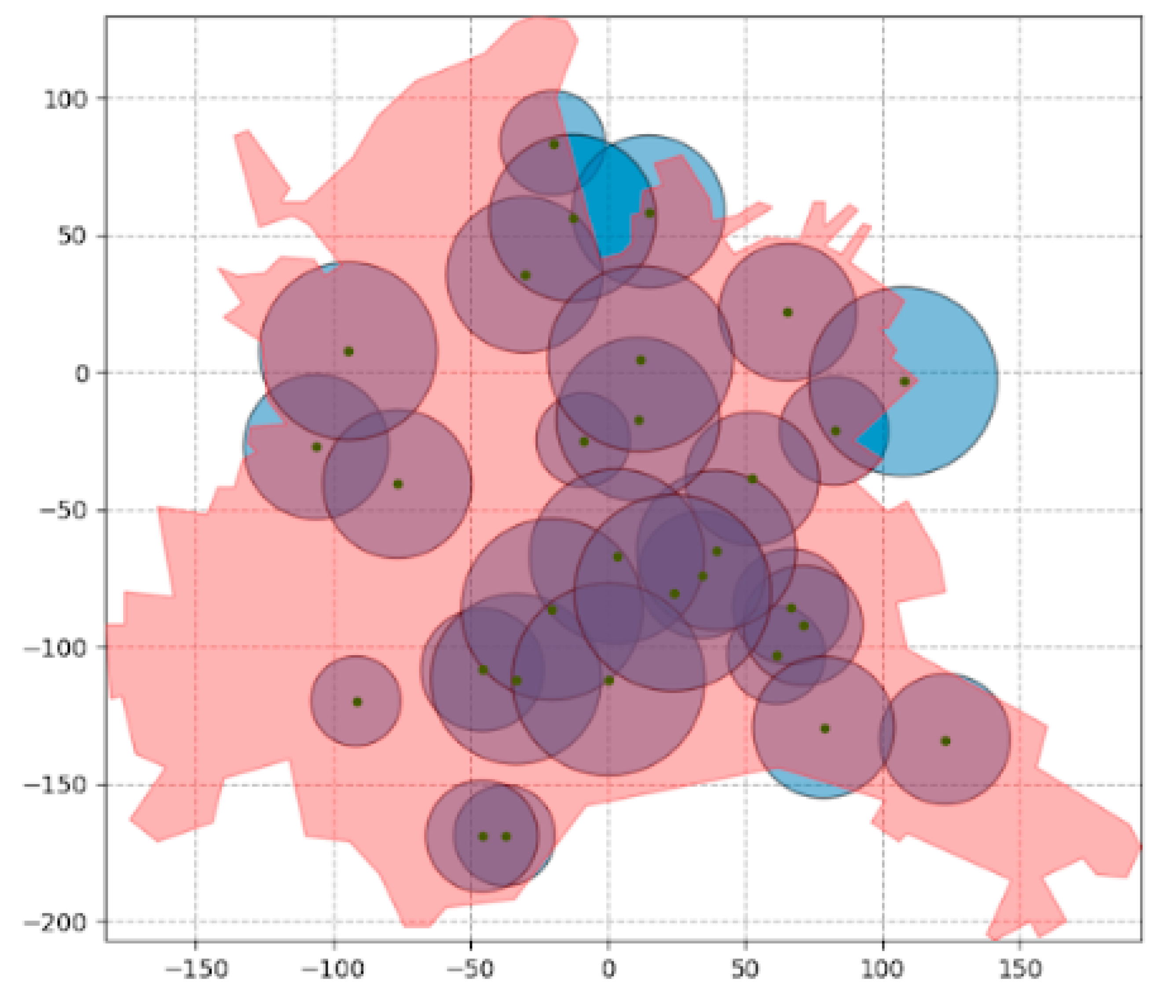
For the global optimization of the function $\mathrm{G}({\mathbf{p}}^1,\dots ,{\mathbf{p}}^{\mathrm{n}})$, a multi-start was used with a random generation of 1000 starting points and the calculation of the corresponding local extrema of $\mathrm{G}({\mathbf{p}}^1,\dots ,{\mathbf{p}}^{\mathrm{n}})$. In Figure 4, one of the typical options for the random location of the 30 circles is given. The placement parameters $({\mathrm{x}}_{\mathrm{i}},{\mathrm{y}}_{\mathrm{i}}),\mathrm{i}\in {\mathrm{N}}_{30}^{}$ corresponding to the best result in the multi-start series are presented in

Table 3. Placement parameters of circular service areas.

$\mathbf{i}$	${\mathbf{x}}_{\mathbf{i}}$	${\mathbf{y}}_{\mathbf{i}}$	$\mathbf{i}$	${\mathbf{x}}_{\mathbf{i}}$	${\mathbf{y}}_{\mathbf{i}}$	$\mathbf{i}$	${\mathbf{x}}_{\mathbf{i}}$	${\mathbf{y}}_{\mathbf{i}}$
1	111.69	−155.55	11	57.71	−75.68	21	−14.28	−12.97
2	27.18	55.03	12	−106.88	−28.94	22	−40.14	96.13
3	22.49	−77.35	13	−60.6	−37.4	23	86.23	−119.34
4	31.88	−5.47	14	−112.58	17.29	24	73.33	−25.82
5	−54.44	−110.27	15	−55.89	−180.46	25	−91.38	−79.68
6	132.77	−128.88	16	−26.74	−141.24	26	−86.17	−141.45
7	17.88	24.89	17	−67.59	4.98	27	26.08	−122.24
8	99.35	−69.99	18	66.21	25.06	28	157.33	−171.10
9	−139.85	−60.41	19	−78.87	57.79	29	−146.76	−113.69
10	24.35	−44.11	20	−27.74	40.84	30	−23.27	−76.61

. The area of the region ${\mathrm{S}}_0$ covered by the services is equal to 60,798.8 units.

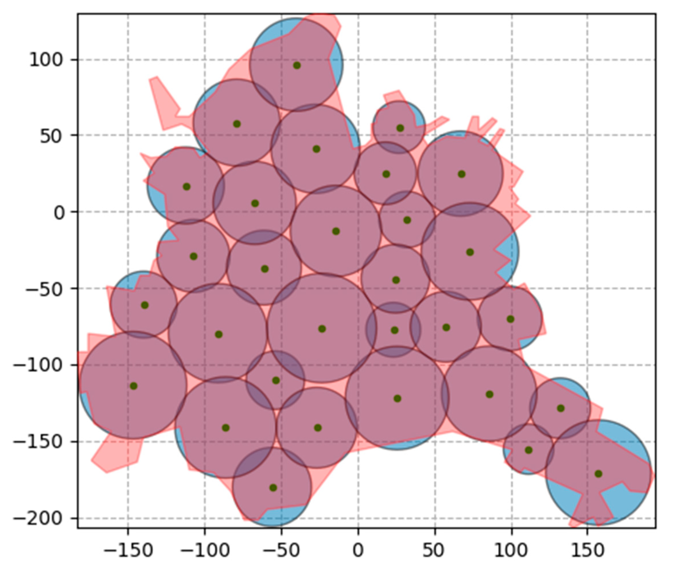
Further improvement by maximizing the function $\mathrm{W}({\mathbf{p}}^1,\dots ,{\mathbf{p}}^{\mathrm{n}})$ made it possible to obtain the solution depicted in Figure 5. Improved circle placement parameters are listed in

Table 4. Improved placement parameters of circular service areas.

$\mathbf{i}$	${\mathbf{x}}_{\mathbf{i}}$	${\mathbf{y}}_{\mathbf{i}}$	$\mathbf{i}$	${\mathbf{x}}_{\mathbf{i}}$	${\mathbf{y}}_{\mathbf{i}}$	$\mathbf{i}$	${\mathbf{x}}_{\mathbf{i}}$	${\mathbf{y}}_{\mathbf{i}}$
1	111.65	−155.55	11	57.54	−75.53	21	−14.17	−12.92
2	27.02	55.06	12	−107.28	−29.20	22	−40.11	95.90
3	23.28	−77.48	13	−61.16	−36.86	23	85.92	−119.26
4	32.30	−5.38	14	−112.24	16.92	24	73.34	−26.23
5	−53.77	−110.50	15	−55.92	−180.31	25	−91.19	−79.70
6	132.31	−128.83	16	−26.76	−141.58	26	−86.19	−141.42
7	18.14	24.85	17	−67.24	5.51	27	25.74	−122.17
8	99.41	−70.13	18	67.17	24.65	28	157.27	−170.88
9	−139.74	−61.05	19	−78.98	58.03	29	−146.69	−113.76
10	24.68	−44.06	20	−27.50	40.83	30	−23.47	−76.35

. The corresponding area of the region ${\mathrm{S}}_0$ covered by the services is equal to 60,806.5 units.

In the process of implementing the approach, the following run time parameters were obtained. For the 30 circles, each local extremum of the function $\mathrm{G}({\mathbf{p}}^1,\dots ,{\mathbf{p}}^{\mathrm{n}})$ was searched for an average of 1.7 s with the random generation of the starting point $({\widehat{\mathbf{p}}}^1,\dots ,{\widehat{\mathbf{p}}}^{\mathrm{n}})$. The multi-start run time of 1000 starting points with subsequent local optimization required 1942 s. The local optimum of the function $\mathrm{W}({\mathbf{p}}^1,\dots ,{\mathbf{p}}^{\mathrm{n}})$ is found to be 1.3 s. In this case, the best solution resulting from the multi-start was taken as the starting point. The fact that the local extremum of a more complex function $\mathrm{W}({\mathbf{p}}^1,\dots ,{\mathbf{p}}^{\mathrm{n}})$ is found to be faster than for $\mathrm{G}({\mathbf{p}}^1,\dots ,{\mathbf{p}}^{\mathrm{n}})$ is explained using a good starting point. As experiments have shown, the average time to obtain a local solution to the function $\mathrm{W}({\mathbf{p}}^1,\dots ,{\mathbf{p}}^{\mathrm{n}})$ in the case of the random generation of the starting point $({\widehat{\mathbf{p}}}^1,\dots ,{\widehat{\mathbf{p}}}^{\mathrm{n}})$ was about 4.9 s. Analysis of the results substantiates the expediency of using an auxiliary problem at the stage of global optimization.

When the items ${\mathrm{S}}_{\mathrm{i}},\mathrm{i}\in {\mathrm{N}}_{\mathrm{n}}^{}$ have the shape of an ellipse, then ${\mathbf{g}}^{\mathrm{i}}=({\widehat{\mathbf{m}}}^{\mathrm{i}},{\mathbf{p}}^{\mathrm{i}})=({\mathrm{a}}_{\mathrm{i}},{\mathrm{b}}_{\mathrm{i}},{\mathrm{x}}_{\mathrm{i}},{\mathrm{y}}_{\mathrm{i}},{\mathsf{\theta }}_{\mathrm{i}})$; where $({\mathrm{a}}_{\mathrm{i}},{\mathrm{b}}_{\mathrm{i}})$ are given semi-major and semi-minor axes, $({\mathrm{x}}_{\mathrm{i}},{\mathrm{y}}_{\mathrm{i}},{\mathsf{\theta }}_{\mathrm{i}})$ are the coordinates of the center in the coordinate system $\mathrm{O}\mathrm{x}\mathrm{y}$. To obtain dependencies ${\mathsf{\omega }}_{{\mathsf{\psi }}_{\mathrm{i}\mathrm{j}}}({\mathbf{g}}^{\mathrm{i}},{\mathbf{g}}^{\mathrm{j}})$, one can use the formulas for the area of the intersection of the two ellipses. Due to the cumbersome nature of these formulas, we do not present them here. Moreover, as shown by numerical experiments, the time for calculating functions ${\mathsf{\omega }}_{{\mathsf{\psi }}_{0\mathrm{j}}}({\widehat{\mathbf{g}}}^0,{\widehat{\mathbf{g}}}^{\mathrm{j}})$ and ${\mathsf{\omega }}_{{\mathsf{\psi }}_{\mathrm{i}\mathrm{j}}}({\mathbf{g}}^{\mathrm{i}},{\mathbf{g}}^{\mathrm{j}})$, $\mathrm{i},\mathrm{j}\in {\mathrm{N}}_{\mathrm{n}}^{}$, $\mathrm{j}>\mathrm{i}$ from analytical formulas is commensurate with the use of computer geometry software.

In this case, the Python code instance for calculating function $\mathrm{G}({\mathbf{p}}^1,\dots ,{\mathbf{p}}^{\mathrm{n}})$ is as follows:

from shapely.geometry.point import Point

from shapely.geometry import Polygon

from shapely import affinity

region = Polygon(region_vert_coord)

ellipses = []

for i in range(n):

 circle = Point(center[i]).buffer(1)

 ellipses.append(affinity.rotate(affinity.scale(circle), a[i], b[i]), angle[i]))

functionG = 0

for i in range(n − 1):

 for j in range(i + 1, n):

  functionG += ellipses[i].intersection(ellipses[j]).area

sum_ellipse_area = 0

for i in range(n):

 functionG -= region.intersection(ellipses[i]).area

 sum_ellipse_area += ellipses[i].area

functionG += sum_ellipse_area

The Python code instance for calculating the function $\mathrm{W}({\mathbf{p}}^1,\dots ,{\mathbf{p}}^{\mathrm{n}})$ looks like this:

region = Polygon(region_vert_coord)

ellipses_loc = []

for i in range(n):

 circle = Point(center[i]).buffer(1)

 ellipses_loc.append(affinity.rotate(affinity.scale(circle), a[i], b[i]), angle[i]))

result_functionW = region.intersection(unary_union(ellipses_loc)).area

Let us consider a test problem similar to the one above but with an ellipse-shaped service area ${\mathrm{S}}_{\mathrm{i}},\mathrm{i}\in {\mathrm{N}}_{30}$. Semi-major and semi-minor axes $({\mathrm{a}}_{\mathrm{i}},{\mathrm{b}}_{\mathrm{i}})$, $\mathrm{i}\in {\mathrm{N}}_{30}^{}$ are presented in

Table 5. Semi-axes of elliptical service areas.

$\mathbf{i}$	ai	bi	$\mathbf{i}$	ai	bi	$\mathbf{i}$	ai	bi	$\mathbf{i}$	ai	bi	$\mathbf{i}$	ai	bi
1	20	35	7	25	33	13	35	20	19	27	34	25	19	34
2	20	27	8	23	37	14	18	20	20	22	36	26	35	21
3	18	22	9	21	30	15	37	16	21	16	35	27	25	26
4	37	18	10	29	32	16	31	18	22	37	18	28	36	26
5	33	30	11	30	24	17	28	34	23	24	37	29	17	36
6	25	31	12	29	20	18	29	22	24	24	17	30	24	36

. The total area of the 30 ellipses is 66,212.2 units.

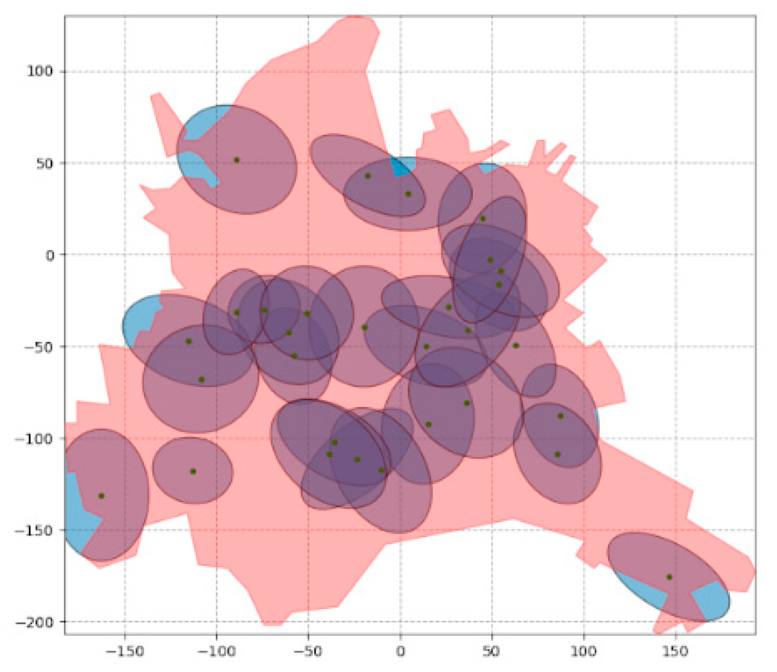
For the global optimization of the function $\mathrm{G}({\mathbf{p}}^1,\dots ,{\mathbf{p}}^{\mathrm{n}})$, a multi-start was used with a random generation of 100 starting points $({\widehat{\mathbf{p}}}^1,\dots ,{\widehat{\mathbf{p}}}^{\mathrm{n}})$ and the calculation of the corresponding local extrema of $\mathrm{G}({\widehat{\mathbf{p}}}^1,\dots ,{\widehat{\mathbf{p}}}^{\mathrm{n}})$. In Figure 6, one of the typical options for the random location of the 30 ellipses is given. The placement parameters $({\mathrm{x}}_{\mathrm{i}},{\mathrm{y}}_{\mathrm{i}},{\mathsf{\theta }}_{\mathrm{i}}),\mathrm{i}\in {\mathrm{N}}_{30}^{}$ corresponding to the best result in the multi-start series are presented in

Table 6. Placement parameters of elliptical service areas.

i	${\mathbf{x}}_{\mathbf{i}}$	${\mathbf{y}}_{\mathbf{i}}$	θi	i	${\mathbf{x}}_{\mathbf{i}}$	yi	θi	i	${\mathbf{x}}_{\mathbf{i}}$	${\mathbf{y}}_{\mathbf{i}}$	θi
1	−34.95	104.68	−4.28	11	−61.40	−171.99	−10.40	21	−59.61	−39.35	−16.59
2	−1.87	−95.03	−5.96	12	−33.31	59.20	41.42	22	31.21	34.27	−7.16
3	−21.11	−147.97	24.78	13	−146.40	−138.11	5.34	23	127.19	−143.53	31.23
4	84.21	−116.46	−10.68	14	99.68	−68.73	10.12	24	−128.23	−60.46	−7.58
5	41.26	−73.69	−11.65	15	−105.27	−101.31	16.64	25	−50.31	−84.73	−8.35
6	−77.48	67.57	−3.84	16	−106.56	24.08	0.23	26	−159.36	−94.27	−11.08
7	79.23	18.52	−13.68	17	−10.29	15.93	−18.56	27	24.47	−22.86	17.74
8	−91.84	−60.45	−1.86	18	−99.77	−143.01	−6.89	28	−15.99	−46.15	−5.19
9	69.01	−31.92	20.14	19	27.73	−125.83	−5.18	29	−54.85	12.48	−15.51
10	−34.95	104.68	−4.28	20	−99.72	−14.36	−5.12	30	160.04	−177.04	−5.87

. The area of the region ${\mathrm{S}}_0$ covered by services is equal to 60,946.5 units.

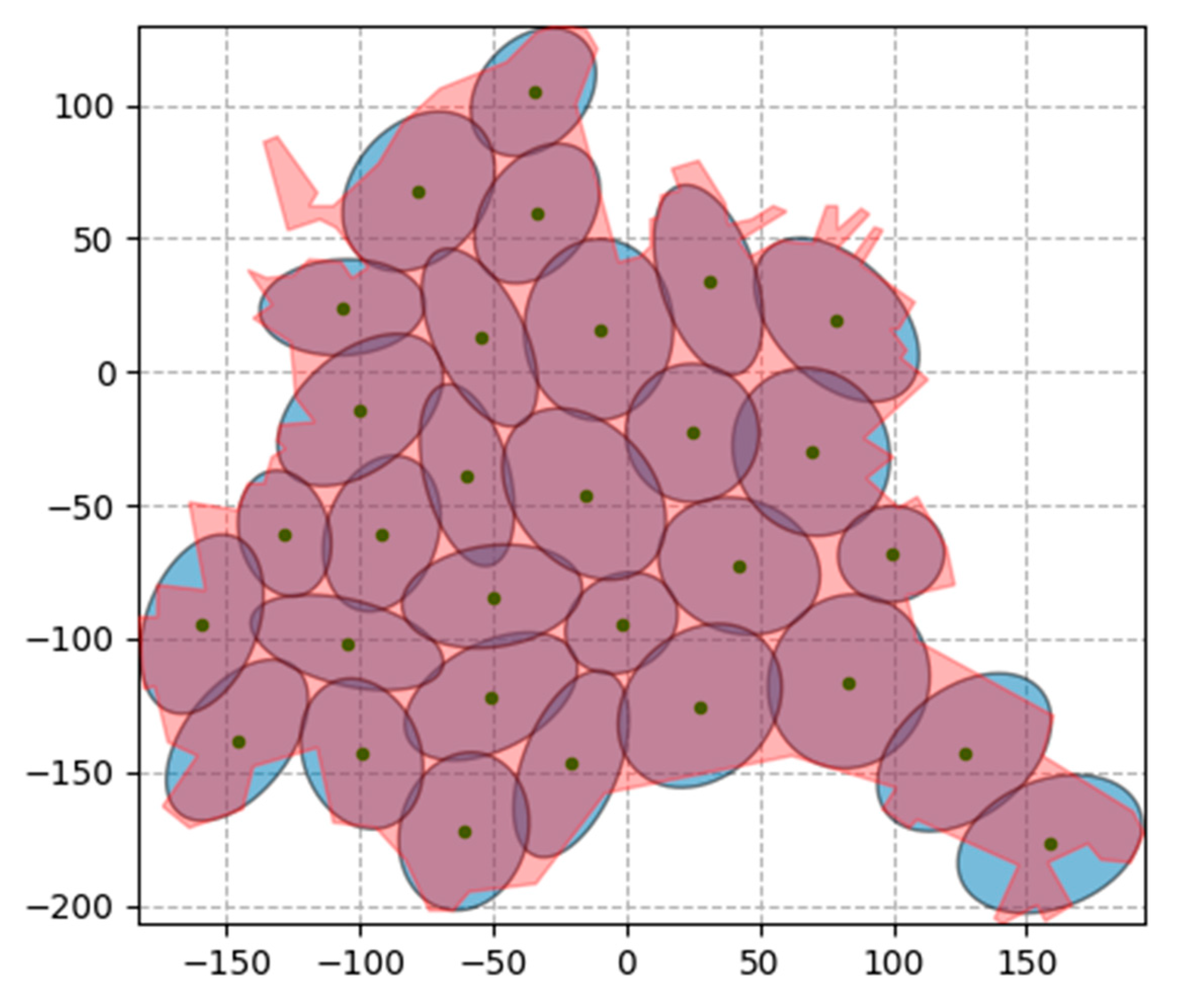
Further improvement by maximizing the function $\mathrm{W}({\mathbf{p}}^1,\dots ,{\mathbf{p}}^{\mathrm{n}})$ allowed us to obtain the location of the service areas shown in Figure 7. Improved ellipses placement parameters are presented in

Table 7. Improved placement parameters of elliptical service areas.

i	${\mathbf{x}}_{\mathbf{i}}$	${\mathbf{y}}_{\mathbf{i}}$	θi	i	${\mathbf{x}}_{\mathbf{i}}$	${\mathbf{y}}_{\mathbf{i}}$	θi	i	${\mathbf{x}}_{\mathbf{i}}$	${\mathbf{y}}_{\mathbf{i}}$	θi
1	−50.81	−121.74	−6.26	11	−61.04	−172.34	−10.51	21	−59.84	−38.8	−16.55
2	−34.98	104.77	−4.28	12	−33.55	59.24	41.37	22	30.68	34.31	−7.24
3	−1.92	−94.24	−6.02	13	−146.03	−138.16	5.22	23	126.63	−142.71	30.82
4	−20.81	−147.09	24.83	14	99.23	−68.43	9.89	24	−128.32	−60.66	−7.56
5	83.36	−116.13	−10.99	15	−104.88	−101.52	16.59	25	−50.47	−84.23	−8.21
6	42.22	−72.88	−11.00	16	−106.63	24.07	0.29	26	−159.29	−94.66	−11.03
7	−77.98	67.56	−3.99	17	−10.44	15.73	−18.26	27	24.68	−22.99	17.99
8	78.78	19.37	−13.46	18	−99.29	−143.28	−6.92	28	−15.91	−45.89	−4.93
9	−91.79	−60.69	−1.84	19	27.48	−125.26	−4.49	29	−55.11	12.73	−15.47
10	69.27	−30.11	20.45	20	−99.88	−14.38	−5.04	30	158.81	−177.09	−6.84

. The corresponding area of the region ${\mathrm{S}}_0$ covered by the services is equal to 60,957.0 units.

For the 30 ellipses, the local extremum of the function $\mathrm{G}({\mathbf{p}}^1,\dots ,{\mathbf{p}}^{\mathrm{n}})$ was searched for an average of 14.5 s with the random generation of the starting point. The multi-start run time of 100 starting points with subsequent local optimization required 1542 s. The local optimum of the function $\mathrm{W}({\mathbf{p}}^1,\dots ,{\mathbf{p}}^{\mathrm{n}})$, when the best solution resulting from the multi-start is chosen as the starting point, was found to be 8.3 s. The average time for finding the local maximum of the function $\mathrm{W}({\mathbf{p}}^1,\dots ,{\mathbf{p}}^{\mathrm{n}})$ in the case of the random generation of the initial starting point is about 25 s.

Thus, the use of an auxiliary problem for the global optimization of the function $\mathrm{W}({\mathbf{p}}^1,\dots ,{\mathbf{p}}^{\mathrm{n}})$ significantly reduces the solution time, and the results are close. The time saved can be used to increase the number of starting points in the multi-start scheme, and therefore to obtain a better solution to the problem as a whole.

4. Discussion

A feature of this article is the study of the maximum service coverage in the business site selection problem in the continuous formulation of the MCLP, taking into account the arbitrary spatial shape of the demand zone and service areas. Traditionally, the demand zone was represented as a set of points due to the limited possibilities of processing the spatial and geometric data of the demand area. The assumption that space can be represented as a discrete set of points potentially leads to an inadequate model. However, demand tends to be distributed continuously, which must be taken into account when modeling business site selection. Accounting for the size and shape of the service area when estimating service coverage results in a more accurate and realistic representation. In this sense, the maximum service coverage problems in terms of the MCLP with items of arbitrary geometric shape is of particular interest. Continuous MCLPs require the construction of special mathematical models and optimization methods that take into account their specifics.

The studies conducted allowed us to approach the analysis of the mathematical model of the problem from a general position, considering geometric features (taking into account the size and shape of the demand zone and service areas). On the one hand, it is possible to set the demand zone and service areas by constructing equations for the boundaries of the corresponding geometric items. On the other hand, you can use computer geometry software to analyze the relative location of these items and calculate service coverage criteria depending on the location of the service areas. An important result that was obtained is the formalization of such criteria and the formulation of the corresponding nonlinear optimization problem. At the same time, the difficulties associated with the analytical specification of the optimality criterion are overcome by using computer geometry packages that work perfectly with geometric items of a complex spatial shape.

The optimization problem under consideration is essentially multidimensional and multiextremal. The authors managed to propose an approach to a fast run time approach for estimating local solutions by introducing an auxiliary problem. As a result, it takes seconds to calculate the objective function and search for its local extremum, which is confirmed by the experiments. For the considered test problems, the multi-start was used to enumerate local solutions. Even in this case, quite good results are obtained. It should be expected that the use of metaheuristic, in particular, evolutionary, methods of global optimization will improve the efficiency of the proposed approach.

The task of determining the location of the service areas that provide the maximum coverage of the demand zone in the general case is the basis for the Maximum Service Coverage in Business Site Selection. In a more general setting, additional problems arise for the optimal location of service centers belonging to the indicated areas. At the same time, it is important not only to fulfill the restrictions on the allowable location of centroids within the service areas but also the mutual location of centroids. Partially, such restrictions are formalized by taking into account the minimum and maximum allowable distances between centroids. Moreover, in the future, routing problems and others related to servicing the centers themselves arise. Thus, in the general case, we have a multi-level and multi-criteria problem, the solution of which is inextricably linked to the quality and time of solving the problem of determining the location of service areas that provide maximum coverage. These tasks, using the approach proposed in the article, are supposed to be studied in the future.

5. Conclusions

As a result of the study, the following innovations were obtained:

• the service coverage model in business site selection was presented as a continuous maximum coverage location problem;
• in this model, the demand zone is also continuous (continuum), in contrast to the known continuous MCLP, where only service area placement parameters (centroid coordinates) are continuous;
• both the demand zone and the service area have an arbitrary shape and different sizes, which is also an extension of the known results;
• our generalized continuous MCLP is formulated as a nonlinear optimization problem, in which the variables are the placement parameters of the service area;
• analytical and algorithmic approaches to the calculation of the objective function are proposed depending on the shape of the demand zone and the service area;
• to solve the problem, an approach is proposed that comprehensively combines the stages of local and global optimization;
• at the stage of local optimization, an auxiliary problem was used based on the decomposition of the objective function, which significantly reduced the computation time;
• numerical experiments confirmed the adequacy of the model and the effectiveness of the proposed approach.