1. Introduction
The implementation of DR programs is sensitive to the consumer’s perception and mentality in relation to a couple of factors that are not always measured directly using tools such as surveys or questionnaires. Confirmatory factor analysis (CFA) is a statistical instrument that allows the testing of hypotheses that are sustained by theory. It requires a good knowledge of the field to identify the latent factors and group the observed variables by those latent factors.
For this investigation, we extracted observed variables from two complex and large questionnaires that targeted Irish electricity consumers during a pre-trial and post-trial period of installing smart metering systems (SMS) in which their consumption and opinions were monitored. The data sets can be accessed (
https://www.ucd.ie/issda/data/commissionforenergyregulationcer/ (accessed on 25 January 2022)) from CER that initiated a project that aimed to evaluate the performance of a couple of DR programs using SMS and tested the opportunity to install more SMS. It consists of two of the largest and most comprehensive trials in the world that are aimed at both residential consumers and small and medium enterprises.
The two 143-item and 243-item questionnaires were launched to residential electricity consumers that were subject to a pre- and post-trial SMS implementation carried out by the Irish CER to test the electricity consumers’ behavior. The questions accounted for numerous latent factors such as demographics (sex, age, education, employment status), attitude, expectation, relation with supplier, perceived impact of their own actions, pro-environmental measures, appliances, heating usage, and perceived implementation of the DR programs. In this article, the research is focused on the residential consumer respondents to the questionnaires that accounted for 4232 observations (pre-trial) and 3423 observations (post-trial). Thus, our study uses the real-life experience of the Irish residential consumers.
Our purpose was to test the structure of the factors underlying the questionnaire data sets. Thus, we empirically test the theory that describes the structure of factors that underlies the two data sets [
1,
2]. Furthermore, this study verifies whether the measurement model created with CFA shows an acceptable fit to the data and shows how it can be modified to be even better. The contribution of this paper consists of the following:
the creation of two measurement models (first-order CFA) that test the structure of factors that are behind the observed variables of the two large and complex questionnaires;
the creation of several hierarchical CFA models, such as second-order and bi-factor models to reflect the relation between the items of the questionnaires and the awareness of electricity consumers;
the testing of the models to prove that they do not capitalize on chance characteristics of the data, proving that the data-model fit is not random, and the model can generalize on different data sets;
drawing interesting conclusions and providing information on the relationship between respondents’ answers and their awareness of environmental issues and implementation of DR programs.
This paper is structured into six sections. In the
Section 1, an introduction to the general context, motivation, and contribution of this paper is provided. In the
Section 2, a comprehensive literature review is performed, while in the
Section 3, the research methodology is presented. We provide an exploratory data analysis (EDA) of the input data in
Section 4. The results and simulations are revealed in
Section 5 along with meaningful discussions on the main findings of this study. The conclusion is drawn in
Section 6.
2. Review of the Literature
Numerous studies use CFA in investigations related to consumer awareness, behavior, education, psychology, economy, etc., in social science research to analyze questionnaire data and to extract valuable insights that are not easy to measure otherwise [
3,
4,
5,
6,
7].
A first wave of studies related to attitudes towards energy consumption and conservation using CFA emerged in the United States in the 1990s [
8] and focused on identifying the dimensions underlying energy usage attitudes, concepts, and beliefs. A total of 308 observations taken from the respondents in Macau were analyzed using CFA and structural equation modelling (SEM) to show that environmental concerns and financial benefits were the factors that influenced the perception of full electric vehicles (FEV) and the intention to purchase FEV. It revealed that the perception of economic benefit was one of the key factors influencing the adoption of FEV [
9].
Furthermore, the authors of [
10] analyzed the responses of 246 electricity consumers from Pakistan using CFA and SEM to measure consumers’ awareness about electricity conservation in developing countries. It measured the influence of some factors such as beliefs, attitudes, and intentions on energy conservation, showing that awareness [
11], perceived value, resistance to change, and benefits were predictors of behavioral changes towards efficient energy conservation measures.
An investigation of the effect of digitalization, climate change and energy consumption of 282 Indonesian respondents using CFA and regression was proposed in [
12]. Awareness of smart technologies increased the experience of consumers.
The factors that impacted the awareness of the residential consumers, perceived benefits, price and attitudes were investigated in [
13] considering 516 respondents from Jordan. Both exploratory and confirmatory factor analyses were carried out to identify the latent factors and to check the performance indicators. The relationship among these factors was also analyzed using SEM. The study found that awareness positively impacted acquisition intentions, perceived gain, and consumption behavior.
Energy saving practices and participation towards renewable energy development were studied in Malaysia using CFA and AMOS software [
14,
15] or with both Exploratory Factor Analysis (EFA) and CFA [
16]. The latter study contained a factor structure that consisted of the degree of knowledge on RES, environmental concern, public awareness on RES, attitude towards RES usage, and willingness to adopt RES technologies and aimed to predict the willingness to pay for green energy.
Furthermore, several case studies were deployed in Tanzania [
17] assessing indicators of energy access in rural areas using both EFA and CFA and concluding that these indicators related to the energy access were significant in improving the social economic progress and the living standards of the people in rural areas of Tanzania.
Another competitive software, LISREL, was exploited in [
18] to study the factors underlying the waste-to-energy facilities in Thailand. A sample of 361 individuals’ responses were analyzed with CFA and the Structural Equation Model (SEM) proving that all factors had a positive influence on the waste-to-energy facilities.
More studies on influencing factors related to energy management in industries [
19], assessing the employees’ engagement in energy-saving [
20], residential consumers’ lifestyle and energy saving [
21], and experience in green energy learning [
22] were recently performed using CFA and sometimes SEM to identify future trends. The authors of [
19] aimed to analyze the influencing factors on energy management in industries from several perspectives with CFA. They analyzed the responses to surveys applied to different industrial sectors in Brazil showing a positive correlation among the factors.
Consumption data and questionnaires deployed by the Irish CER were involved in obtaining a clustering solution [
23], the classification of load profiles [
24,
25], extracting insights from smart metering data and responses of electricity consumers [
26], anomaly detection [
27], and forecasts [
28,
29,
30].
Although numerous studies have been conducted with consumption data and questionnaires deployed by the Irish CER, to our knowledge, the two large questionnaires with 3000–4000 respondents and 150–250 items have not yet been analyzed with CFA.
3. Research Methodology
The research methodology implemented in this article consisted of processing large and challenging data sets for CFA. First, we split the questions of each questionnaire into significant groups that revealed specific characteristics of electricity consumers and their consumption. The pre-trial questionnaire consisted of 4232 observations and 143 questions that were grouped by 7 variables summing up data on: q1 Demographics, q2 Positive attitude, q3 Negative attitude, q4 Pro-environmental measures, q5 Expectations, q6 Relation with supplier, and q7 Appliances. These variables were further grouped by 2 latent factors: F1 social–economic and F2 behavioral factors.
On the other hand, the post-trial questionnaire had 3423 observations and 234 questions that were grouped by 9 variables that summed up data about: q1 DR program, q2 Demographics, q3 Positive attitude, q4 Negative attitude, q5 Heating, q6 Pro-environmental measures, q7 Positive perception on price-based DR implementation, q8 Negative perception on price-based DR implementation, and q9 Perception of incentive-based DR. Each observed variable was influenced by one latent factor and a measurement error. For CFA, the SAS CALIS procedure was implemented using the lineqs statement that allowed us to define the observed variables as linear equations. Similar results could be obtained with a factor statement that is similar to lineqs.
In the
lineqs statement, we defined a set of linear equations for each observed variable
. It is equal to the factor loading
multiplied by latent factor
plus a measurement error or residual term
.
where
i is the number of observed variables and
k is the number of latent factors. Using
variance and
covariance (cov) statements, we defined the variances and covariances that were calculated using the CALIS procedure. Variances for latent factors were set to 1, whereas they were allowed to covary, and the covariance was defined in the
cov statement.
The pathdiagram statement allowed us to display the CFA diagram along with the main performance indicators. When using the
factor statement, the relationships are written as:
where
j is the number of variables that load on a certain latent factor
.
We set on the residual robust and modification options of the CALIS procedure. As we summed up the answers for a series of questions, the problem with the missing value disappeared, but outliers still existed and lowered the performance indicators of the model. They are printed with the plots = caseresid option of the CALIS procedure. Therefore, residual robust is an option for outlier treatment that does not simply erase or remove some outliers that may lead to a masking effect. It is an alternative way to handle outliers that are down-weighed simultaneously with the estimation. The observations are iteratively reweighted based on the updated parameter estimates. The performance of the model increases with the residual robust option from Comparative Fit Index (CFI) = 0.9, Standardized Root Mean Squared Residual (SRMR) = 0.05 and Root Mean Square Error of Approximation (RMSEA) = 0.08 to CFI = 0.91, SRMR = 0.4 and RMSEA = 0.07. The modification option is also important, as it may provide meaningful suggestions to improve the model.
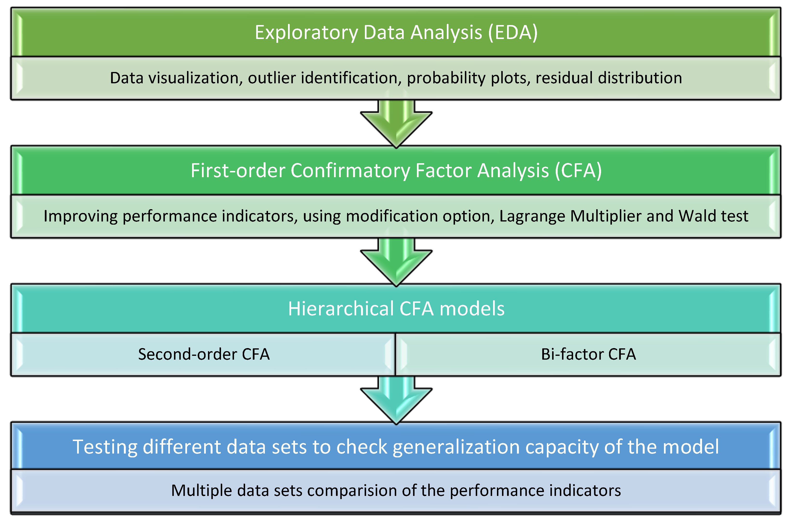
The methodology of this research study consisted of the following steps (as in
Figure 1): (1) first, an exploratory data analysis (EDA) was performed to visualize the data distribution and identify outliers to further treat them and help improve the model performance; (2) the first-order CFA was initially performed with the
modification option on to check whether there was additional room for improvement. The Lagrange Multiplier and Wald tests were included in the
modification option. However, these modifications were moderately approached and verified with the theory; (3) third, more complex CFA models were created to verify if the performance indicators could be further improved. Moreover, these models (second-order CFA and bi-factor models) allowed us to consider one or more latent factors that were not easy to measure in questionnaires; (4) forth, more tests were performed to prove that the models did not capitalize on chance in a data set and they could provide good results with other data sets as well.
4. EDA of Input Data
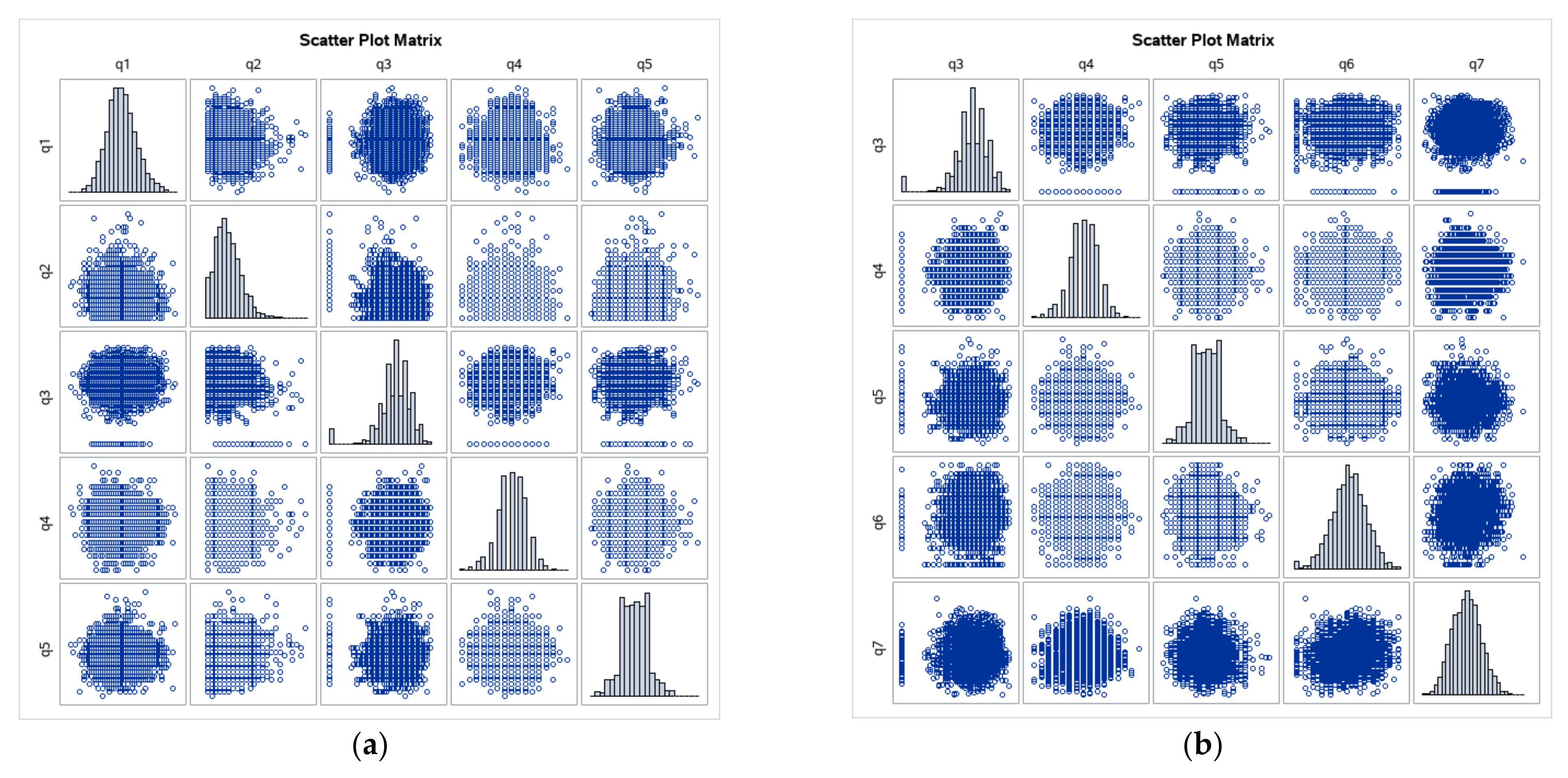
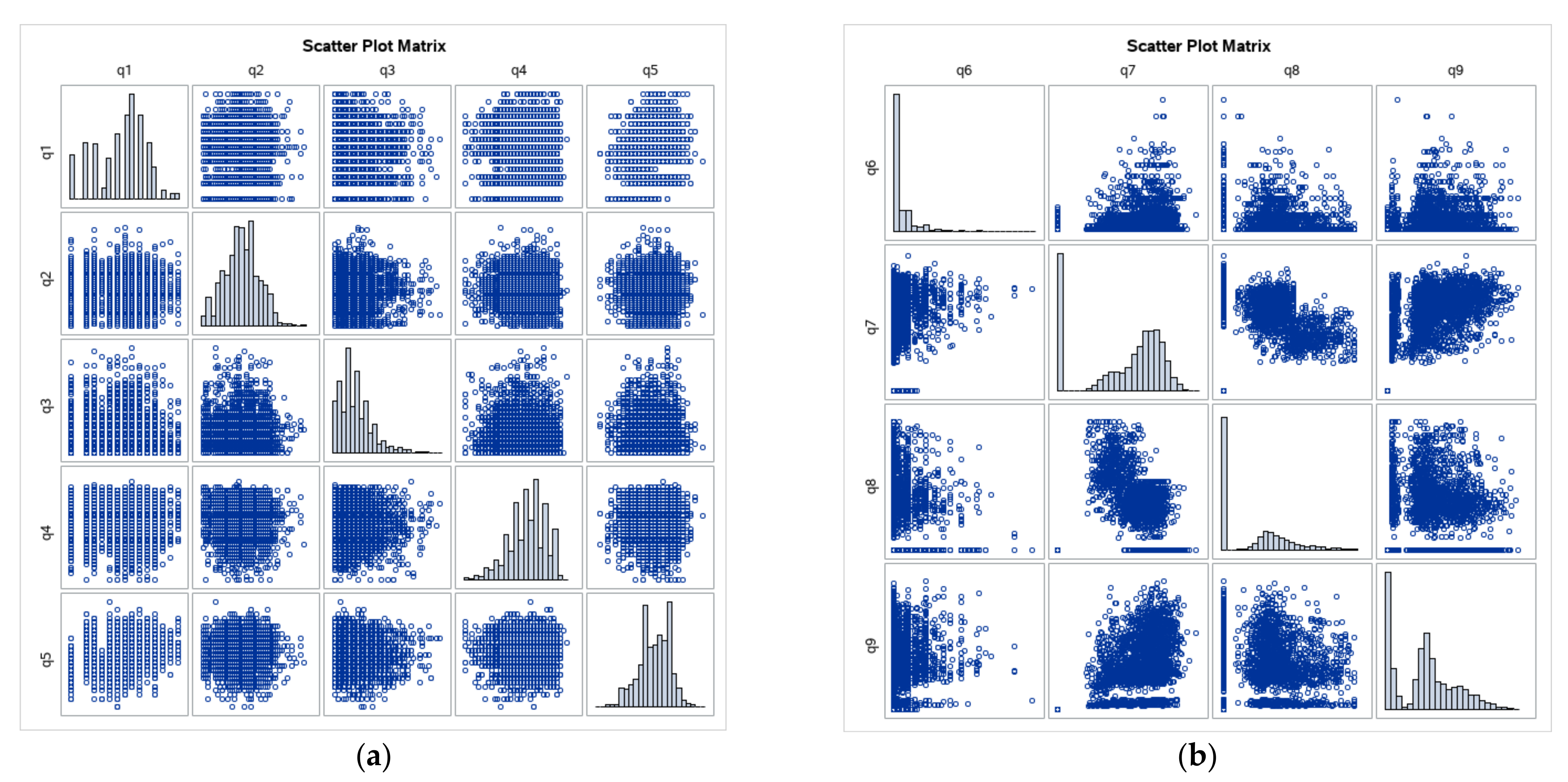
Both data sets are analyzed in this section. A similar EDA was performed for each of them. The pre-trial questionnaire data set consisted of seven derived variables, whereas the post-trial questionnaire data set had nine variables that were scatter plotted to display their distribution (as in
Figure 2 and
Figure 3).
The pre-trial variables were closer to the normal distribution than the post-trial variables. Thus, the logarithm function could be applied to the post-trial variables.
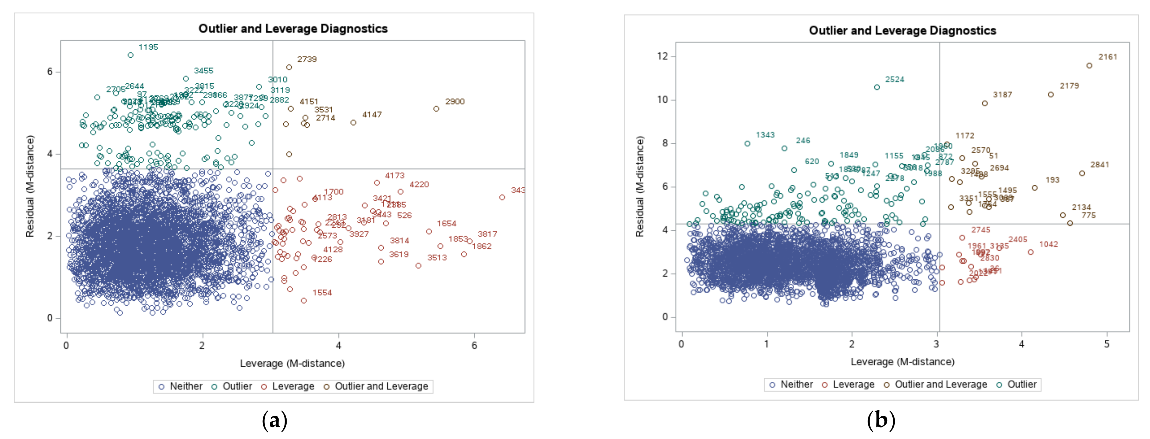
Outliers generally decreased the performance of CFA. Therefore, the values were grouped into normal and outliers as in
Figure 4.
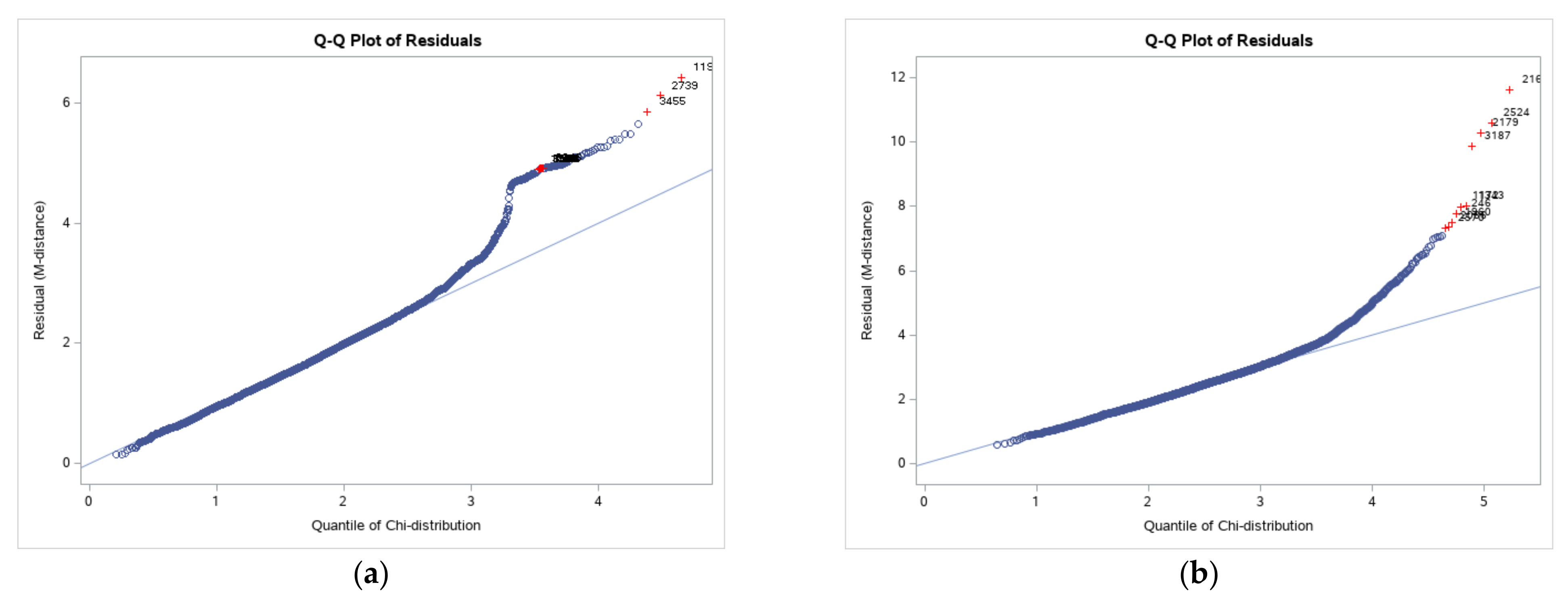
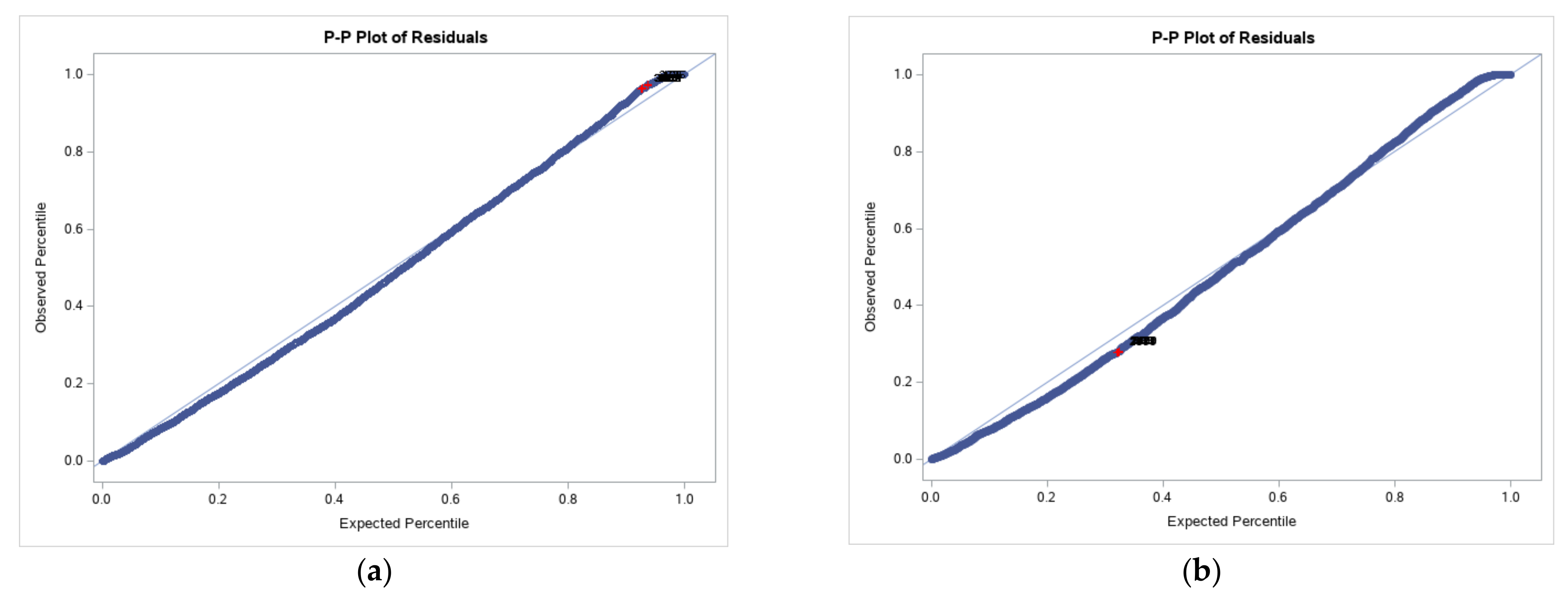
Probability graphs are displayed to assess whether a data set was approximately normally distributed. The data were plotted against a theoretical normal distribution so that the points should have formed a straight line. Departures from it indicate departures from normality that were more evident for the post-trial data set (as in
Figure 5 and
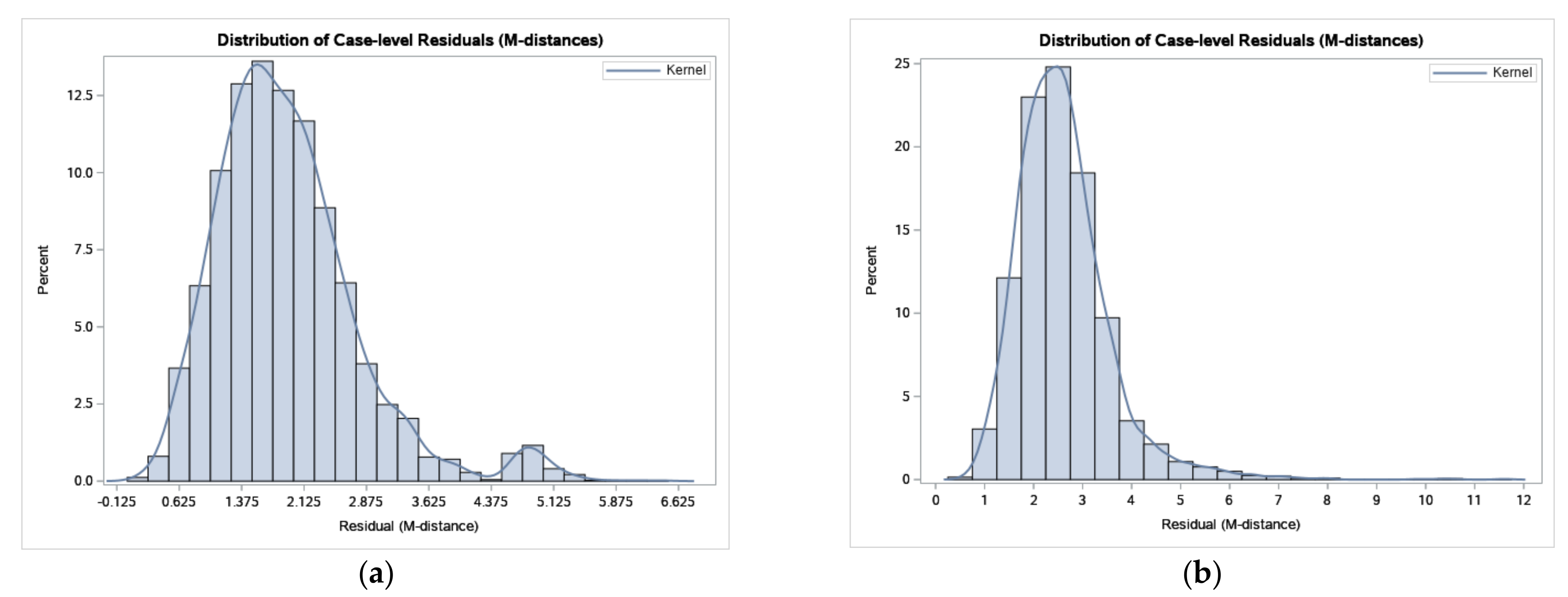
Figure 6). The distributions of the residuals are provided in
Figure 7.
With the p-p plots, we obtained a higher resolution in the center of the distribution. On the other hand, with the q-q plots, we obtained a higher resolution at the tails. We were more concerned about the tails of a distribution, which impacted the model.
5. Results
The numerous items of the pre-trial questionnaire were aggregated into seven observed variables: q1 for Demographics, q2 for Positive attitude, q3 for Negative attitude, q4 for Measures, q5 for Expectations, q6 for Relation with supplier, and q7 for Appliances. Two latent factors were considered: F1 as the social–economic factor and F2 as the behavioral factor. Variables q1, q4, q6, and q7 from the pre-trial questionnaire loaded on the social–economic factor (F1), while q2, q3, and q5 loaded on the behavioral factor (F2). The SAS CALIS procedure was implemented for the pre-trial questionnaire as in
Table 1. The
Lineqs statement was considered to define the variables as linear equations. Each observed variable was influenced by its latent factor and measurement error.
Nine variables were extracted from the post-trial questionnaire: q1 for the DR program, q2 for Demographics, q3 for Positive attitude, q4 for Negative attitude, q5 for Heating, q6 for Measures, q7 for Positive perception on price-based DR implementation, q8 for Negative perception on price-based DR implementation, and q9 for Perception on incentive-based DR. The same two latent factors were considered: F1 as the social–economic factor and F2 as the behavioral factor. Variables q2, q5, and q6 from the post-trial questionnaire loaded on the social-economic factor (F1), while q1, q3, q4, q7–q9 loaded on the behavioral factor (F2). Furthermore, the CALIS procedure was implemented for the data set of the post-trial questionnaire as in
Table 2 using the
lineqs statement to define the nine variables.
The results related to the modelling information and variables are presented in
Table 3 and
Table 4. The mean and standard deviation for the observed variables are presented in
Table 5.
After 12 iterations, the convergence was reached for the first-order CFA model run on the pre-trial data set (as in
Table 6), whereas only 6 iterations were required for the post-trial data set (as in
Table 7).
The factor loadings for the pre-trial questionnaire and the post-trial questionnaire are presented in
Table 8 and
Table 9. In each case, there was one factor loading that was not statistically significant, p4 for the pre-trial questionnaire for which the
t value was outside the limits (that is smaller than 2.58) and p2 for the post-trial questionnaire for which the
t value was 1.289, which was also less than 2.58.
Based on the Wald test (as in
Table 10), we removed the two factor loadings that were also indicated in
Table 8 and
Table 9 as not statistically significant. Therefore, the q4 variable was removed from the pre-trial data set and the simulation was repeated.
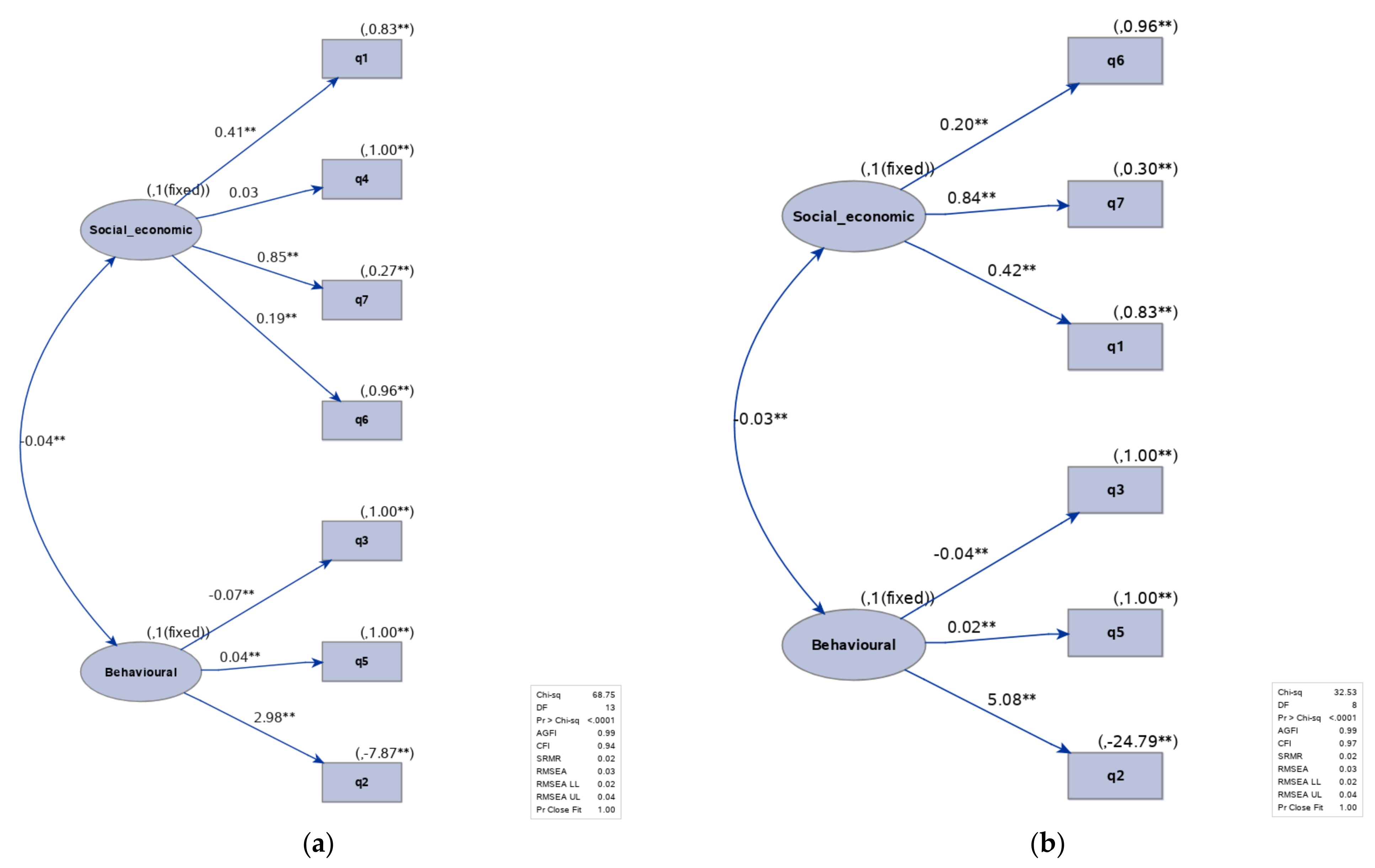
In
Figure 8, the two path diagrams for the pre-trial data set are displayed before and after modification option. The q4 variable did not load on F1 (social–economic factor) and CFI improved from 0.94 to 0.97, which indicates a better fit.
Furthermore, from the above path diagrams we may conclude that there was a weak correlation between the two latent factors. A synthesis of the performance indicators is shown in each diagram that reveals that apart from CFI and chi-square that decreased, the other indicators remained unchanged. In
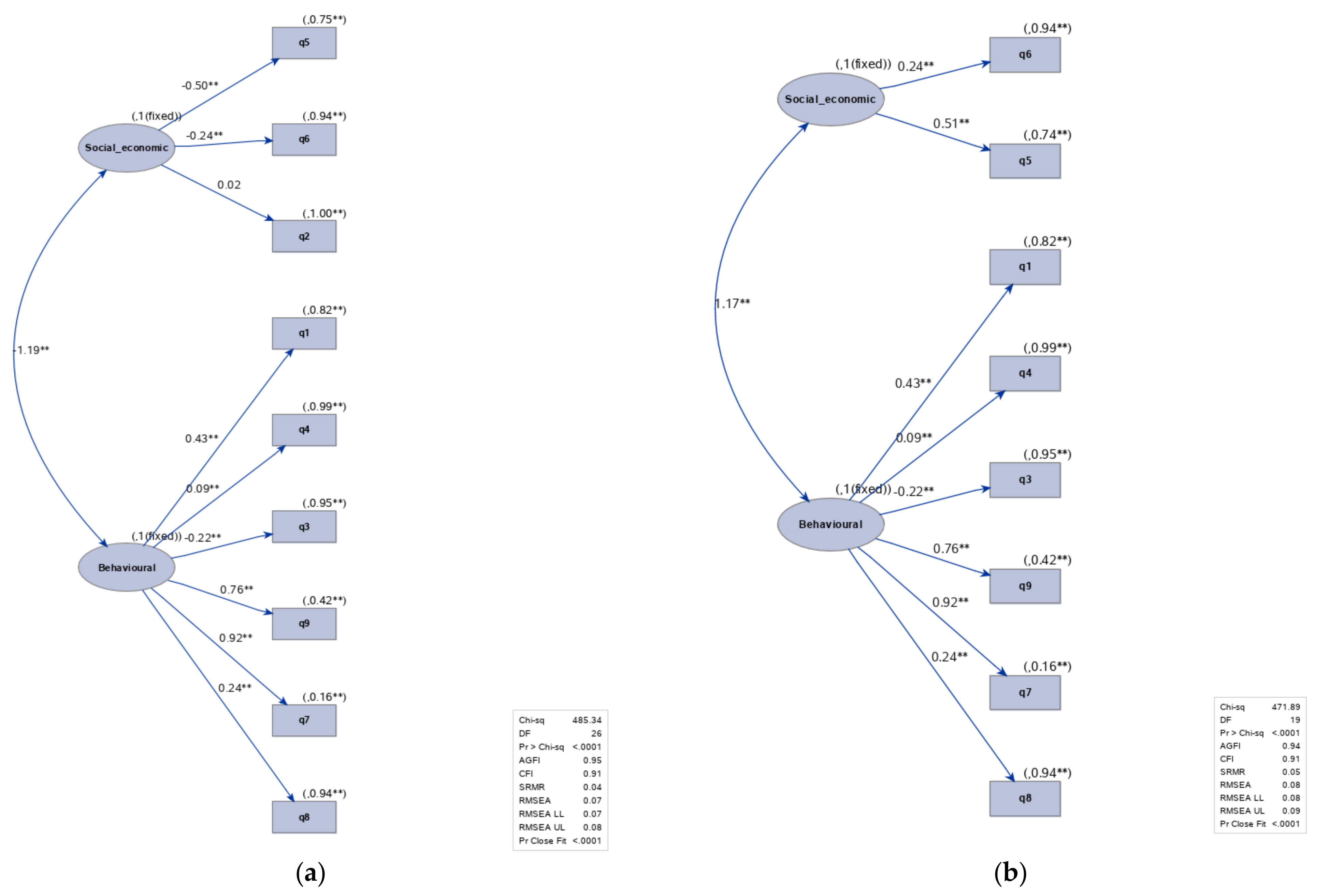
Figure 9, the two path diagrams for the post-trial data set are displayed before and after modification. At first sight, we noticed that the chi-square was much larger than in the previous model.
However, when q2 was removed from the post-trial data set, the performance indicators did not improve. On the contrary, RMSEA and SRMR increased by 0.01. In addition to the performance indicators that are displayed along with the path diagrams, all indicators are displayed in
Table 11 for the two models with and without modification indicated by the Wald test. Some other modifications were suggested by the Lagrange Multiplier test, but they were not reasonable from the theory point of view.
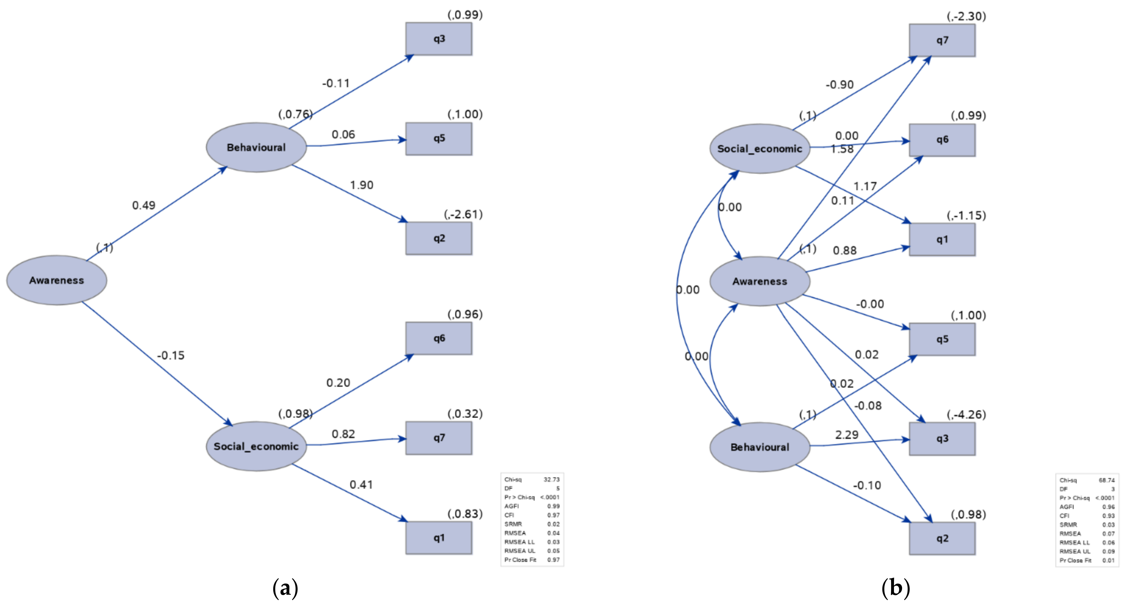
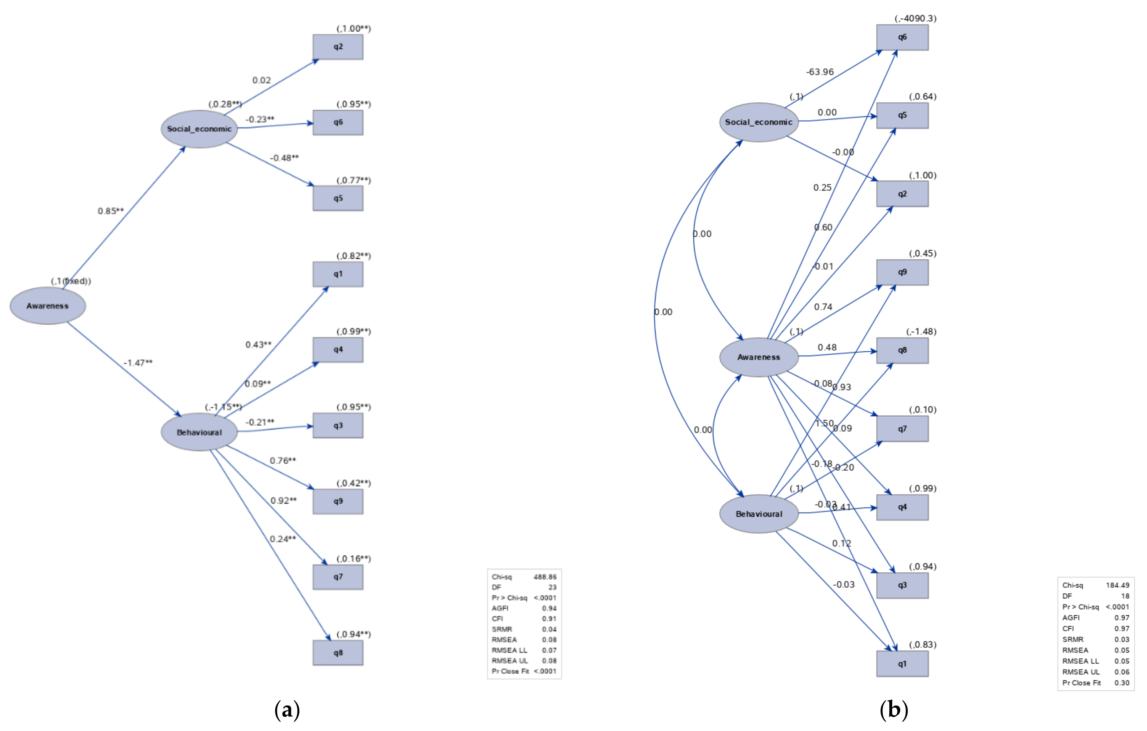
Furthermore, two hierarchical models were created for the two data sets. These complex models allowed us to insert a new latent variable ‘Awareness’ that could be affected by social–economic and behavioral factors (as in
Figure 10 and
Figure 11). In the second-order CFA model, social–economic and behavioral factors were the first-order latent factors, while awareness was the second-order latent factor. The first-order factors acted as an intermediary layer between the second-order factor and observed variables. On the contrary, in the case of the bi-factor model, the observed variables loaded on two factors (one group and one general factor).
Comparable results were obtained with the second-order CFA for the pre-trial data set, whereas better results were obtained with the bi-factor model for the post-trial data set, improving CFI from 0.91 to 0.97, SRMR from 0.04 to 0.03, and RMSEA from 0.07 to 0.05.
The challenge with CFA models and small data sets is that the model can perform well only for a single data set. However, when the data set is large, it can be divided into subsets, and the CFA models can be run on each of them to check whether the model is capable of generalizing different data sets or if it just capitalizes on chance in a data set. The size of the data set must have enough statistical power that can be tested using the degrees of freedom of the model and the sample size. With 4232 observations and DF = 8, the statistical power was 0.99, while with 1058 observations, the statistical power was 0.83, which was higher than 0.8, indicating the reliable statistical power of the data sample. Thus, the 4232 observations of the pre-trial data set were divided into four data subsets of 1058 observations each creating the first, second, third and fourth data subsets as in
Table 12. We noticed that with smaller data sets, the chi-square was smaller, and the probability was even smaller than 0.05, which confirmed the null hypothesis that the theoretical model fit the data. This is a proper demonstration of the fact that the chi-square is sensitive to the data sample size and is not always reliable to indicate an adequate fit to data, especially when the data set is large (as the pre-trial data set).
6. Conclusions
Very good results in terms of performance indicators from each category (absolute, parsimony and incremental indexes) were obtained for the pre-trial data set with over 4000 respondents, especially when the q4 variable was removed (CFI = 0.97, SRMR = 0.02, RMSEA = 0.03), whereas the results for the post-trial data set were acceptable without excluding variables q2 (CFI = 0.91, SRMR = 0.04 and RMSEA = 0.07). Thus, the modification indications must be tested, and should be in line with the theory that underlies the model.
By considering smaller data subsets, we demonstrated that the chi-square is sensitive to sample size. Furthermore, applying CFA for smaller data sets proved that the model is able to generalize and provide a reliable solution for various data sets.
Implementing more complex hierarchical models brough better or comparable results for both the pre-trial data set (second-order CFA) and the post-trial data set (bi-factor model).
The analyses will be continued as future work with tests of more complex models such as the structural equation model to make further predictions and to understand the relationship among the latent factors.
Author Contributions
Conceptualization, S.-V.O., A.B. and C.-E.C.; methodology, S.-V.O. and A.B.; software, S.-V.O.; validation, C.-E.C., L.F.S. and A.B.; formal analysis, A.B., C.-E.C. and L.F.S.; investigation, L.F.S.; resources, L.F.S.; data curation, A.B. and L.F.S.; writing—original draft preparation, A.B., L.F.S., C.-E.C. and S.-V.O.; writing—review and editing, A.B. and S.-V.O.; visualization, A.B., C.-E.C. and L.F.S.; supervision, A.B. and S.-V.O.; project administration, S.-V.O.; funding acquisition, L.F.S. All authors have read and agreed to the published version of the manuscript.
Funding
This research received no external funding.
Data Availability Statement
Acknowledgments
This work was supported by a grant of the Romanian Ministry of Research and Innovation, CCCDI–UEFISCDI, project number 462PED/28.10.2020, project code PN-III-P2-2.1-PED-2019-1198, within PNCDI III. We would like to address special thanks to the authors of the first two references (Norm O’Rouke, Larry Hatcher and Timothy Brown) and SAS guidelines from SAS Help Center for offering us plenty of informational support.
Conflicts of Interest
The authors declare no conflict of interest.
References
- O’Rourke, N.; Psych, R.; Hatcher, L. A Step-by-Step Approach to Using SAS for Factor Analysis and Structural Equation Modeling; Sas Institute: Cary, NC, USA, 2013; ISBN 978-1-55544-643-7. [Google Scholar]
- Brown, T. Confirmatory Factor Analysis for Applied Research, 2nd ed.; Guilford Publications: New York, NY, USA, 2015; ISBN 146251779X, 9781462517794. [Google Scholar]
- Nurhayati, R. Measuring Students’ Curiosity Character Using Confirmatory Factor Analysis. Eur. J. Educ. Res. 2021, 10, 773–783. [Google Scholar] [CrossRef]
- Bianchi, R.; Schonfeld, I.S.; Verkuilen, J. A Five-Sample Confirmatory Factor Analytic Study of Burnout-Depression Overlap. J. Clin. Psychol. 2020, 76, 801–821. [Google Scholar] [CrossRef] [PubMed]
- Zainudin, M.; Subali, B. Construct Validity of Mathematical Creativity Instrument: First-Order and Second-Order Confirmatory Factor Analysis. Int. J. Instr. 2019, 12, 595–614. [Google Scholar] [CrossRef]
- Selvaraj, S.; Naing, N.N.; Wan-Arfah, N.; Prasadh, S. Confirmatory Factor Analysis of Knowledge, Attitude, and Behaviour Questionnaire towards Oral Health among Indian Adults. J. Pers. Med. 2021, 11, 320. [Google Scholar] [CrossRef]
- Rasool, S.; Rehman, A.; Cerchione, R.; Centobelli, P. Evaluating Consumer Environmental Behavior for Sustainable Development: A Confirmatory Factor Analysis. Sustain. Dev. 2021, 29, 318–326. [Google Scholar] [CrossRef]
- Samuelson, C.D.; Biek, M. Attitudes toward Energy Conservation: A Confirmatory Factor Analysis. J. Appl. Soc. Psychol. 1991, 21, 549–568. [Google Scholar] [CrossRef]
- Lai, I.K.W.; Liu, Y.; Sun, X.; Zhang, H.; Xu, W. Factors Influencing the Behavioural Intention towards Full Electric Vehicles: An Empirical Study in Macau. Sustainability 2015, 7, 12564–12585. [Google Scholar] [CrossRef] [Green Version]
- Habib, M.D.; Shah, H.J.; Qayyum, A. Analyzing the Role of Values, Beliefs and Attitude in Developing Sustainable Behavioral Intentions: Empirical Evidence from Electric Power Industry. Bus. Econ. Rev. 2021, 13, 19–44. [Google Scholar] [CrossRef]
- Trotta, G. Electricity Awareness and Consumer Demand for Information. Int. J. Consum. Stud. 2021, 45, 65–79. [Google Scholar] [CrossRef]
- Sasmoko, S.; Mihardjo, L.W.W.; Alamsjah, F.; Elidjen, E.; Tarofder, A.K. Investigating the effect of digital technologies, energy consumption and climate change on customer’s experience: A study from Indonesia. Int. J. Energy Econ. Policy 2019, 9, 353–362. [Google Scholar] [CrossRef] [Green Version]
- Akroush, M.N.; Zuriekat, M.I.; Al Jabali, H.I.; Asfour, N.A. Determinants of Purchasing Intentions of Energy-Efficient Products: The Roles of Energy Awareness and Perceived Benefits. Int. J. Energy Sect. Manag. 2019, 13, 128–148. [Google Scholar] [CrossRef]
- Hanifah, M.; Mohmadisa, H.; Nasir, N.; Yazid, S.; Saiyidatina Balkhis, N. A Confirmatory Factor Analysis of Malaysian Primary School Students’ Energy Saving Practices. J. Turkish Sci. Educ. 2018, 15, 51–63. [Google Scholar] [CrossRef]
- Mahat, H.; Hashim, M.; Saleh, Y.; Nayan, N.; Norkhaidi, S.B. Factor Analysis on Energy Saving Knowledge among Primary School Students in Malaysia: A Case Study in Batang Padang District, Perak. Kasetsart J. Soc. Sci. 2019, 40, 448–453. [Google Scholar] [CrossRef]
- Abdullah, W.M.Z.B.W.; Zainudin, W.N.R.A.B.; Ishak, W.W.B.M.; Sulong, F.B.; Zia Ul Haq, H.M. Public Participation of Renewable Energy (Ppred) Model in Malaysia: An Instrument Development. Int. J. Renew. Energy Dev. 2020, 10, 119–137. [Google Scholar] [CrossRef]
- Mangula, M.S.; Kuzilwa, J.A.; Msanjila, S.S.; Legonda, I.A. Indicators of Energy Access in Rural Areas of Tanzania: An Application of Confirmatory Factor Analysis Approach. Indep. J. Manag. Prod. 2018, 9, 1068–1078. [Google Scholar] [CrossRef] [Green Version]
- Chailertpong, T.; Phimolsathien, T. Antecedents to Creating Shared Value at Thai Waste-to-Energy Facilities. J. Sustain. Dev. Energy Water Environ. Syst. 2018, 6, 649–664. [Google Scholar] [CrossRef] [Green Version]
- Sola, A.V.H.; Mota, C.M.M. Influencing Factors on Energy Management in Industries. J. Clean. Prod. 2020, 248, 119263. [Google Scholar] [CrossRef]
- Chen, C.H.V.; Chen, Y.C. Assessment of Enhancing Employee Engagement in Energy-Saving Behavior at Workplace: An Empirical Study. Sustainability 2021, 13, 2457. [Google Scholar] [CrossRef]
- Thøgersen, J. Housing-Related Lifestyle and Energy Saving: A Multi-Level Approach. Energy Policy 2017, 102, 73–87. [Google Scholar] [CrossRef]
- Hong, J.C.; Tsai, C.R.; Hsiao, H.S.; Chen, P.H.; Chu, K.C.; Gu, J.; Sitthiworachart, J. The Effect of the “Prediction-Observation-Quiz-Explanation” Inquiry-Based e-Learning Model on Flow Experience in Green Energy Learning. Comput. Educ. 2019, 133, 127–138. [Google Scholar] [CrossRef]
- Gorzalczany, M.B.; Piekoszewski, J.; Rudzinski, F. Electricity Consumption Data Clustering for Load Profiling Using Generalized Self-Organizing Neural Networks with Evolving Splitting-Merging Structures. In Proceedings of the IEEE International Symposium on Industrial Electronics, Cairns, QLD, Australia, 13–15 June 2018. [Google Scholar]
- Lin, S.; Gu, X.; Tang, J.; Li, D.; Fu, Y. Power Load Profile Classification Method Based on Neural Network of Sparse Automatic Encoder. Dianwang Jishu Power Syst. Technol. 2020, 44, 3508–3515. [Google Scholar] [CrossRef]
- Wang, Y.; Bennani, I.L.; Liu, X.; Sun, M.; Zhou, Y. Electricity Consumer Characteristics Identification: A Federated Learning Approach. IEEE Trans. Smart Grid 2021, 12, 3637–3647. [Google Scholar] [CrossRef]
- Oprea, S.V.; Bâra, A.; Tudorică, B.G.; Călinoiu, M.I.; Botezatu, M.A. Insights into Demand-Side Management with Big Data Analytics in Electricity Consumers’ Behaviour. Comput. Electr. Eng. 2021, 89, 106902. [Google Scholar] [CrossRef]
- Oprea, S.V.; Bâra, A.; Puican, F.C.; Radu, I.C. Anomaly Detection with Machine Learning Algorithms and Big Data in Electricity Consumption. Sustainability 2021, 13, 10963. [Google Scholar] [CrossRef]
- Lungu, I.; Bâra, A.; Cărutasu, G.; Pîrjan, A.; Oprea, S.V. Prediction Intelligent System in the Field of Renewable Energies through Neural Networks. Econ. Comput. Econ. Cybern. Stud. Res. 2016, 50, 85–102. [Google Scholar]
- Vrablecová, P.; Bou Ezzeddine, A.; Rozinajová, V.; Šárik, S.; Sangaiah, A.K. Smart Grid Load Forecasting Using Online Support Vector Regression. Comput. Electr. Eng. 2018, 65, 102–117. [Google Scholar] [CrossRef]
- Kiruithiga, D.; Manikandan, V. Time Series Load Forecasting Using Pooling Based Multitasking Deep Neural Network. In Proceedings of the 2021 IEEE Power and Energy Society Innovative Smart Grid Technologies Conference (ISGT), Washington, DC, USA, 16–18 February 2021. [Google Scholar]
Figure 1.
Research methodology.
Figure 1.
Research methodology.
Figure 2.
Scatter plot and distribution of variables (a) q1–q5, (b) q3–q7 of the pre-trial data set.
Figure 2.
Scatter plot and distribution of variables (a) q1–q5, (b) q3–q7 of the pre-trial data set.
Figure 3.
Scatter plot and distribution of variables (a) q1–q5, (b) q6–q9 of the post-trial data set.
Figure 3.
Scatter plot and distribution of variables (a) q1–q5, (b) q6–q9 of the post-trial data set.
Figure 4.
Outliers (a) pre-trial data set and (b) post-trial data set.
Figure 4.
Outliers (a) pre-trial data set and (b) post-trial data set.
Figure 5.
Q-Q plot of residuals (a) pre-trial data set and (b) post-trial data set.
Figure 5.
Q-Q plot of residuals (a) pre-trial data set and (b) post-trial data set.
Figure 6.
P-P plot of residuals (a) pre-trial data set, (b) post-trial data set.
Figure 6.
P-P plot of residuals (a) pre-trial data set, (b) post-trial data set.
Figure 7.
Distribution of residuals (a) pre-trial data set, (b) post-trial data set.
Figure 7.
Distribution of residuals (a) pre-trial data set, (b) post-trial data set.
Figure 8.
Path diagrams for the data set of the pre-trial questionnaire (a) initial (b) after modification.
Figure 8.
Path diagrams for the data set of the pre-trial questionnaire (a) initial (b) after modification.
Figure 9.
Path diagrams for the post-trial questionnaire data set (a) initial (b) after modification.
Figure 9.
Path diagrams for the post-trial questionnaire data set (a) initial (b) after modification.
Figure 10.
Path diagrams for the pre-trial questionnaire data set (a) second-order, (b) bi-factor.
Figure 10.
Path diagrams for the pre-trial questionnaire data set (a) second-order, (b) bi-factor.
Figure 11.
Path diagrams for the post-trial questionnaire data set (a) second-order, (b) bi-factor.
Figure 11.
Path diagrams for the post-trial questionnaire data set (a) second-order, (b) bi-factor.
Table 1.
CALIS implementation of the first-order CFA model for the pre-trial questionnaire.
Table 1.
CALIS implementation of the first-order CFA model for the pre-trial questionnaire.
| data preq7factor; | variance |
| infile ‘/home/simonaoprea0/preq7factor.csv’ dsd; | e1-e7 = vare1-vare7, |
| input id $ q1-q7; | F1 = 1, F2 = 1; |
| run; | cov |
| proc calis modification residual robust; | F1 F2 = covF1F2; |
| lineqs | var q1-q7; |
| q1 = p1 F1 + e1, | pathdiagram diagram = standard |
| q2 = p2 F2 + e2, | scale = 0.75 EXOGCOVARIANCE |
| q3 = p3 F2 + e3, | label = [F1 = “Social_economic” |
| q4 = p4 F1 + e4, | F2 = “Behavioural”] |
| q5 = p5 F2 + e5, | dh = 1000 dw = 1000 |
| q6 = p6 F1 + e6, | textsizemin = 10; |
| q7 = p7 F1 + e7; | run; |
Table 2.
CALIS implementation of the first-order CFA model for the pre-trial questionnaire.
Table 2.
CALIS implementation of the first-order CFA model for the pre-trial questionnaire.
| data post9factor; | q9 = p9 F2 + e9; |
| infile ‘/home/simonaoprea0/post9factor.csv’ dsd; | variance |
| input id $ q1 q2 q3 q4 q5 q6 q7 q8 q9; | e1−e9 = vare1−vare9, |
| run; | F1 = 1, F2 = 1; |
| proc calis modification residual robust; | cov |
| lineqs | F1 F2 = covF1F2; |
| q1 = p1 F2 + e1, | var q1−q9; |
| q2 = p2 F1 + e2, | pathdiagram diagram = standard scale = 0.75 EXOGCOVARIANCE |
| q3 = p3 F2 + e3, | label = [F1 = “Social_economic” F2 = “Behavioural”] dh = 1000 dw = 1000 textsizemin = 10; |
| q4 = p4 F2 + e4, | run; |
| q5 = p5 F1 + e5, | - |
| q6 = p6 F1 + e6, | - |
| q7 = p7 F2 + e7, | - |
| q8 = p8 F2 + e8, | - |
Table 3.
Modelling information.
Table 3.
Modelling information.
| Modelling Information for Pre-Trial Questionnaire | Modelling Information for Post-Trial Questionnaire |
|---|
| Modeling Information | Modeling Information |
|---|
| Robust Maximum Likelihood Estimation | Robust Maximum Likelihood Estimation |
|---|
| Data Set | WORK.PREQ7FACTOR | Data Set | WORK.POST9FACTOR |
| N Records Read | 4232 | N Records Read | 3423 |
| N Records Used | 4232 | N Records Used | 3423 |
| N Obs | 4232 | N Obs | 3423 |
| Model Type | LINEQS | Model Type | LINEQS |
| Analysis | Means and Covariances | Analysis | Means and Covariances |
Table 4.
Variables information.
Table 4.
Variables information.
| Variables for the Pre-Trial Questionnaire | Variables for the Post-Trial Questionnaire |
|---|
| Variables in the Model | Variables in the Model |
|---|
| Number of Endogenous Variables = 7 | Number of Endogenous Variables = 9 |
| Number of Exogenous Variables = 9 | Number of Exogenous Variables = 11 |
| Endogenous | Manifest | q1 q2 q3 q4 q5 q6 q7 | Endogenous | Manifest | q1 q2 q3 q4 q5 q6 q7 q8 q9 |
| | Latent | - | | Latent | |
| Exogenous | Manifest | - | Exogenous | Manifest | |
| - | Latent | F1 F2 | - | Latent | F1 F2 |
| - | Error | e1 e2 e3 e4 e5 e6 e7 | - | Error | e1 e2 e3 e4 e5 e6 e7 e8 e9 |
Table 5.
Simple statistics for the two data sets.
Table 5.
Simple statistics for the two data sets.
| Simple Statistics for the Pre-Trial Questionnaire | Simple Statistics for the Post-Trial Questionnaire |
|---|
| Simple Statistics | Simple Statistics |
|---|
| Variable | Mean | Std Dev | Variable | Mean | Std Dev |
|---|
| q1 | 45.91966 | 6.49056 | q1 | 8.53754 | 3.22219 |
| q2 | 16.78474 | 3.06561 | q2 | 20.61846 | 7.10923 |
| q3 | 23.94849 | 6.01536 | q3 | 16.0894 | 5.63135 |
| q4 | 13.99669 | 2.05743 | q4 | 25.89833 | 5.57182 |
| q5 | 15.60562 | 3.16985 | q5 | 23.71458 | 3.84094 |
| q6 | 18.40052 | 4.01145 | q6 | 3.43003 | 4.67816 |
| q7 | 50.69565 | 11.09745 | q7 | 70.04061 | 41.94054 |
| - | q8 | 17.14607 | 19.24341 |
| - | q9 | 52.78761 | 42.62345 |
Table 6.
Iterations of the first-order CFA model run on the pre-trial data set.
Table 6.
Iterations of the first-order CFA model run on the pre-trial data set.
| Iteration | Restarts | Function
Calls | Active
Constraints | Objective
Function | Objective
Function
Change | Max Abs
Gradient
Element | Lambda | Ratio
between
Actual
and
Predicted
Change |
|---|
| 1 | 0 | 4 | 0 | 0.01052 | 0.00650 | 0.00488 | 0 | 0.936 |
| 2 | 0 | 7 | 0 | 0.00975 | 0.000769 | 0.00411 | 0.0105 | 0.883 |
| 3 | 0 | 10 | 0 | 0.00937 | 0.000377 | 0.00415 | 0.00506 | 0.926 |
| 4 | 0 | 13 | 0 | 0.00919 | 0.000181 | 0.00281 | 0.00334 | 0.940 |
| 5 | 0 | 16 | 0 | 0.00910 | 0.000089 | 0.00248 | 0.00197 | 0.918 |
| 6 | 0 | 19 | 0 | 0.00906 | 0.000046 | 0.00170 | 0.00133 | 0.946 |
| 7 | 0 | 22 | 0 | 0.00903 | 0.000022 | 0.000901 | 0.00111 | 0.983 |
| 8 | 0 | 24 | 0 | 0.00903 | 5.733 × 10⁻⁶ | 0.00379 | 0.00008 | 0.338 |
| 9 | 0 | 26 | 0 | 0.00901 | 0.000015 | 0.000491 | 0 | 1.041 |
| 10 | 0 | 28 | 0 | 0.00901 | 5.027 × 10⁻⁷ | 0.000056 | 0 | 1.173 |
| 11 | 0 | 30 | 0 | 0.00901 | 3.296 × 10⁻⁸ | 0.000031 | 0 | 1.270 |
| 12 | 0 | 32 | 0 | 0.00901 | 2.903 × 10⁻⁹ | 7.566 × 10⁻⁶ | 0 | 1.290 |
Table 7.
Iterations of the first-order CFA model run on the post-trial data set.
Table 7.
Iterations of the first-order CFA model run on the post-trial data set.
| Iteration | Restarts | Function
Calls | Active
Constraints | Objective
Function | Objective
Function
Change | Max Abs
Gradient
Element | Lambda | Ratio
between
Actual
and
Predicted
Change |
|---|
| 1 | 0 | 4 | 0 | 0.15703 | 0.0224 | 0.0292 | 0 | 1.159 |
| 2 | 0 | 6 | 0 | 0.15603 | 0.000998 | 0.00164 | 0 | 1.148 |
| 3 | 0 | 8 | 0 | 0.15599 | 0.000043 | 0.00103 | 0 | 1.129 |
| 4 | 0 | 10 | 0 | 0.15599 | 2.589 × 10⁻⁶ | 0.000035 | 0 | 1.072 |
| 5 | 0 | 12 | 0 | 0.15599 | 1.681 × 10⁻⁷ | 0.000077 | 0 | 0.991 |
| 6 | 0 | 14 | 0 | 0.15599 | 1.187 × 10⁻⁸ | 9.588 × 10⁻⁶ | 0 | 0.905 |
Table 8.
Factor loadings for the pre-trial questionnaire data set.
Table 8.
Factor loadings for the pre-trial questionnaire data set.
| Standardized Effects in Linear Equations for Pre-Trial Questionnaire |
|---|
| Variable | Predictor | Parameter | Estimate | Standard Error | t Value | Pr > |t| |
|---|
| q1 | F1 | p1 | 0.40652 | 0.03209 | 12.6685 | <0.0001 |
| q2 | F2 | p2 | 2.97743 | 0.02871 | 103.7 | <0.0001 |
| q3 | F2 | p3 | −0.06694 | 0.00504 | −13.2872 | <0.0001 |
| q4 | F1 | p4 | 0.03290 | 0.01791 | 1.8370 | 0.0662 |
| q5 | F2 | p5 | 0.03640 | 0.00503 | 7.2344 | <0.0001 |
| q6 | F1 | p6 | 0.19495 | 0.02102 | 9.2762 | <0.0001 |
| q7 | F1 | p7 | 0.85228 | 0.06165 | 13.8250 | <0.0001 |
Table 9.
Factor loadings for the post-trial questionnaire data set.
Table 9.
Factor loadings for the post-trial questionnaire data set.
| Standardized Effects in Linear Equations for Post-Trial Questionnaire |
|---|
| Variable | Predictor | Parameter | Estimate | Standard Error | t Value | Pr > |t| |
|---|
| q1 | F2 | p1 | 0.42884 | 0.01515 | 28.3030 | <0.0001 |
| q2 | F1 | p2 | 0.01971 | 0.01529 | 1.2890 | 0.1974 |
| q3 | F2 | p3 | −0.21572 | 0.01739 | −12.4069 | <0.0001 |
| q4 | F2 | p4 | 0.09304 | 0.01801 | 5.1659 | <0.0001 |
| q5 | F1 | p5 | −0.50338 | 0.03143 | −16.0161 | <0.0001 |
| q6 | F1 | p6 | −0.23909 | 0.02111 | −11.3272 | <0.0001 |
| q7 | F2 | p7 | 0.91882 | 0.00804 | 114.3 | <0.0001 |
| q8 | F2 | p8 | 0.24149 | 0.01719 | 14.0458 | <0.0001 |
| q9 | F2 | p9 | 0.76306 | 0.00965 | 79.1111 | <0.0001 |
Table 10.
Wald test indication.
Table 10.
Wald test indication.
| Wald Test for Pre-Trial Questionnaire | Wald Test for Post-Trial Questionnaire |
|---|
| Stepwise Multivariate Wald Test | Stepwise Multivariate Wald Test |
|---|
| Parm | Cumulative Statistics | Univariate Increment | Parm | Cumulative Statistics | Univariate Increment |
| Chi-Square | DF | Pr > ChiSq | Chi-Square | Pr > ChiSq | Chi-Square | DF | Pr > ChiSq | Chi-Square | Pr > ChiSq |
| p4 | 3.3704 | 1 | 0.0664 | 3.3704 | 0.0664 | p2 | 1.6603 | 1 | 0.1976 | 1.6603 | 0.1976 |
Table 11.
Performance indicators of the first-order CFA model.
Table 11.
Performance indicators of the first-order CFA model.
| Index Category | Performance Indicator | PRE | PREq4 | POST | POSTq2 |
|---|
| Absolute Index | Fit Function | 0.0162 | 0.0077 | 0.1418 | 0.1379 |
| - | Chi-Square | 68.74 | 32.53 | 485.33 | 471.88 |
| Chi-Square DF | 13 | 8 | 26 | 19 |
| Pr > Chi-Square | <0.0001 | <0.0001 | <0.0001 | <0.0001 |
| Z-Test of Wilson and Hilferty | 5.8077 | 3.7435 | 17.9693 | 17.8397 |
| Hoelter Critical N | 1377 | 2017 | 275 | 219 |
| Root Mean Square Residual (RMR) | 0.4779 | 0.5003 | 8.2502 | 9.0782 |
| Standardized RMR (SRMR) | 0.0241 | 0.0189 | 0.0443 | 0.0486 |
| Goodness of Fit Index (GFI) | 0.9955 | 0.9974 | 0.9701 | 0.9674 |
| Parsimony Index | Adjusted GFI (AGFI) | 0.9902 | 0.9933 | 0.9482 | 0.9382 |
| - | Parsimonious GFI | 0.6162 | 0.5320 | 0.7006 | 0.6564 |
| RMSEA Estimate | 0.0318 | 0.0269 | 0.0719 | 0.0835 |
| RMSEA Lower 90% Confidence Limit | 0.0247 | 0.0177 | 0.0663 | 0.0770 |
| RMSEA Upper 90% Confidence Limit | 0.0394 | 0.0369 | 0.0775 | 0.0901 |
| Probability of Close Fit | 1.0000 | 1.0000 | <0.0001 | <0.0001 |
| ECVI Estimate | 0.0234 | 0.0138 | 0.1530 | 0.1479 |
| ECVI Lower 90% Confidence Limit | 0.0181 | 0.0105 | 0.1331 | 0.1282 |
| ECVI Upper 90% Confidence Limit | 0.0304 | 0.0189 | 0.1750 | 0.1697 |
| Akaike Information Criterion | 98.74 | 58.53 | 523.33 | 505.88 |
| Bozdogan CAIC | 209.00 | 154.08 | 658.96 | 627.23 |
| Schwarz Bayesian Criterion | 194.00 | 141.08 | 639.96 | 610.23 |
| McDonald Centrality | 0.9934 | 0.9971 | 0.9351 | 0.9360 |
| Incremental Index | Bentler Comparative Fit Index | 0.9440 | 0.9744 | 0.9125 | 0.9141 |
| - | Bentler-Bonett NFI | 0.9323 | 0.9665 | 0.9082 | 0.9110 |
| Bentler-Bonett Non-normed Index | 0.9095 | 0.9519 | 0.8788 | 0.8734 |
| Bollen Normed Index Rho1 | 0.8907 | 0.9372 | 0.8728 | 0.8688 |
| Bollen Non-normed Index Delta2 | 0.9444 | 0.9745 | 0.9127 | 0.9142 |
| James et al. Parsimonious NFI | 0.5772 | 0.5155 | 0.6559 | 0.6182 |
Table 12.
Results with different data sets.
Table 12.
Results with different data sets.
| - | - | Complete Data Set | 1st Subset | 2nd Subset | 3rd Subset | 4th Subset |
|---|
| Absolute Index | Fit Function | 0.0077 | 0.0219 | 0.0131 | 0.0071 | 0.0109 |
| - | Chi-Square | 32.53 | 23.1501 | 13.8552 | 7.5028 | 11.4965 |
| Chi-Square DF | 8 | 8 | 8 | 8 | 8 |
| Pr > Chi-Square | <0.0001 | 0.0032 | 0.0856 | 0.4835 | 0.1751 |
| Z-Test of Wilson and Hilferty | 3.7435 | 2.7168 | 1.3721 | 0.0397 | 0.9375 |
| Hoelter Critical N | 2017 | 709 | 1184 | 2185 | 1426 |
| Root Mean Square Residual (RMR) | 0.5003 | 0.6682 | 0.5539 | 0.4711 | 0.7003 |
| Standardized RMR (SRMR) | 0.0189 | 0.0296 | 0.0239 | 0.0166 | 0.0226 |
| Goodness of Fit Index (GFI) | 0.9974 | 0.9927 | 0.9956 | 0.9976 | 0.9965 |
| Parsimony Index | Adjusted GFI (AGFI) | 0.9933 | 0.9808 | 0.9884 | 0.9938 | 0.9907 |
| - | Parsimonious GFI | 0.5320 | 0.5294 | 0.5310 | 0.5321 | 0.5314 |
| RMSEA Estimate | 0.0269 | 0.0423 | 0.0263 | 0.0000 | 0.0203 |
| RMSEA Lower 90% Confidence Limit | 0.0177 | 0.0228 | 0.0000 | 0.0000 | 0.0000 |
| RMSEA Upper 90% Confidence Limit | 0.0369 | 0.0630 | 0.0490 | 0.0346 | 0.0444 |
| Probability of Close Fit | 1.0000 | 0.7037 | 0.9580 | 0.9978 | 0.9822 |
| ECVI Estimate | 0.0138 | 0.0467 | 0.0379 | 0.0319 | 0.0356 |
| ECVI Lower 90% Confidence Limit | 0.0105 | 0.0365 | 0.0324 | 0.0324 | 0.0324 |
| ECVI Upper 90% Confidence Limit | 0.0189 | 0.0641 | 0.0516 | 0.0419 | 0.0482 |
| Akaike Information Criterion | 58.53 | 49.1501 | 39.8552 | 33.5028 | 37.4965 |
| Bozdogan CAIC | 154.08 | 126.6839 | 117.3890 | 111.0365 | 115.0303 |
| Schwarz Bayesian Criterion | 141.08 | 113.6839 | 104.3890 | 98.0365 | 102.0303 |
| McDonald Centrality | 0.9971 | 0.9929 | 0.9972 | 1.0002 | 0.9983 |
| Incremental Index | Bentler Comparative Fit Index | 0.9744 | 0.9433 | 0.9754 | 1.0000 | 0.9870 |
| - | Bentler-Bonett NFI | 0.9665 | 0.9180 | 0.9452 | 0.9711 | 0.9596 |
| Bentler-Bonett Non-normed Index | 0.9519 | 0.8938 | 0.9539 | 1.0038 | 0.9757 |
| Bollen Normed Index Rho1 | 0.9372 | 0.8463 | 0.8973 | 0.9459 | 0.9242 |
| Bollen Non-normed Index Delta2 | 0.9745 | 0.9448 | 0.9761 | 1.0020 | 0.9873 |
| James et al. Parsimonious NFI | 0.5155 | 0.4896 | 0.5041 | 0.5179 | 0.5118 |
| Publisher’s Note: MDPI stays neutral with regard to jurisdictional claims in published maps and institutional affiliations. |
© 2022 by the authors. Licensee MDPI, Basel, Switzerland. This article is an open access article distributed under the terms and conditions of the Creative Commons Attribution (CC BY) license (https://creativecommons.org/licenses/by/4.0/).


