
CondNAS: Neural Architecture Search for Conditional CNNs


Department of Electrical and Computer Engineering, University of Seoul, Seoul 02504, Korea
*
Author to whom correspondence should be addressed.
Electronics 2022, 11(7), 1101; https://doi.org/10.3390/electronics11071101
Submission received: 9 March 2022
/
Revised: 27 March 2022
/
Accepted: 28 March 2022
/
Published: 31 March 2022
(This article belongs to the Collection Deep Learning for Computer Vision: Algorithms, Theory and Application)
Abstract
:As deep learning has become prevalent and adopted in various application domains, the need for efficient convolution neural network (CNN) inference on diverse target platforms has increased. To address the need, a neural architecture search (NAS) technique called once-for-all, or OFA, which aims to efficiently find the optimal CNN architecture for the given target platform using genetic algorithm (GA), has recently been proposed. Meanwhile, a conditional CNN architecture, which allows early exits with auxiliary classifiers in the middle of a network to achieve efficient inference without accuracy loss or with negligible loss, has been proposed. In this paper, we propose a NAS technique for the conditional CNN architecture, CondNAS, which efficiently finds a near-optimal conditional CNN architecture for the target platform using GA. By attaching auxiliary classifiers through adaptive pooling, OFA’s SuperNet is successfully extended, such that it incorporates the various conditional CNN sub-networks. In addition, we devise machine learning-based prediction models for the accuracy and latency of an arbitrary conditional CNN, which are used in the GA of CondNAS to efficiently explore the large search space. The experimental results show that the conditional CNNs from CondNAS is 2.52× and 1.75× faster than the CNNs from OFA for Galaxy Note10+ GPU and CPU, respectively.
1. Introduction
The need for efficient deep learning inference on diverse embedded mobile platforms has increased recently. Many applications require real-time object detection and recognition, including autonomous driving, intelligent surveillance, and augmented reality on diverse platforms: cars, robots, drones, smartphones, and various IoT devices. To meet stringent constraints, efficient yet accurate deep learning inference on embedded mobile devices has been actively researched in many directions, including quantization [1], lightweight convolution neural networks (CNNs) [2,3,4], and efficient convolution algorithms [5].
One approach is a neural architecture search (NAS) for diverse platforms. While the traditional NAS techniques only aimed at increasing the classification accuracy not considering the computing platforms [6,7,8,9,10,11], many recent NAS techniques [12,13,14] attempt to find an optimal CNN architecture that can minimize latency of the CNN inference on a given target platform while maintaining the accuracy. The recently proposed NAS technique, once-for-all (OFA) [15], can efficiently search for the optimal CNN through genetic algorithm (GA) without retraining.
Another approach for efficient yet accurate CNN inference is a conditional CNN where a CNN model has auxiliary classifier(s) in the middle of the network, allowing for early exit if it is confident enough to classify the input [16,17,18]. It can avoid forwarding the input (i.e., computing the feature maps) to the end layer, saving time and energy, without sacrificing accuracy if the confidence level was set correctly. The recently proposed work, BPNet [19], can find out the locations to attach the auxiliary classifiers and the threshold of each auxiliary classifier in a systematic manner using GA. Given the target platform and a CNN, it finds the optimal conditional CNN architecture for the platform. Even if BPNet does not alter the base CNN architecture but only determines the location and threshold of each auxiliary classifier, it can be considered a NAS technique that can find fast yet accurate conditional CNN architectures for the target platform.
In this paper, we propose a NAS technique for conditional CNNs to address the problem of fast yet accurate inference on diverse embedded platforms. To the best of our knowledge, no prior work exists for the NAS of conditional CNNs. BPNet can be thought of as a NAS technique for conditional CNNs but it can only find the optimal conditional CNN architectures for the given base network: it cannot alter the base network in the search. One may think of applying BPNet to the CNN obtained by NAS techniques such as OFA. However, it would not be optimal as auxiliary classifier architectures and the base architectures are searched separately in sequence. To consider the auxiliary classifiers simultaneously in the same search process, we propose to integrate the two NAS techniques, OFA and BPNet. The challenges in integrating the two NAS techniques are two-fold. First, how to attach the auxiliary classifiers to the SuperNet in OFA and how many to attach should be considered. SuperNet is a network that contains various parameters that OFA searches. Second, the accuracy and latency predictors for a conditional CNN should be devised. In BPNet, the accuracy and latency are not predicted but directly measured in the profiling phase, and the information is used in the pruning, or the design space exploration (DSE) phase, to find the optimal locations and the thresholds of auxiliary classifiers. However, the GA in the integrated NAS would be too time-consuming if such a direct profiling is employed to evaluate the accuracy and latency.
This paper presents CondNAS, a NAS framework for conditional CNNs, to tackle these two challenges. The SuperNet is extended such that it incorporates auxiliary classifiers through adaptive pooling, and the accuracy and latency prediction models are devised and trained using the dataset of arbitrary conditional CNNs extracted from the extended SuperNet. With the prediction models, the GA can efficiently search the huge design space composed of arbitrary CNN configurations and arbitrary auxiliary classifier configurations. The experimental results show that the conditional CNNs from CondNAS is 2.52× and 1.75× faster than the CNNs from OFA for Galaxy Note10+ GPU and CPU, respectively. Overall, this work makes the following contributions:
- To the best of our knowledge, this is the first NAS technique for the conditional CNNs with different base networks; BPNet is for the same base network.
- Careful extension of the SuperNet with auxiliary classifiers that does not incur accuracy loss
- Accurate prediction models for the accuracy and latency of conditional CNNs.
- Efficient dataset generation to train the prediction models.
- Significant speedups from the (near-)optimal solutions found by CondNAS.
2. Background
2.1. OFA
Once-for-all, or OFA, is a GA-based NAS technique [15] where the model training stage and the neural architecture search stage are decoupled. A once-for-all network that is trained considering diverse architectural configurations, and then (near-)optimal sub-networks for the target platforms are efficiently searched using GA. Two key enablers are the design and training of once-for-all network, or SuperNet, and the accuracy and latency predictors used in GA to extract optimal sub-networks, or SubNets, for the target platform from the trained SuperNet. Thanks to these, the NAS cost for the N different platforms and devices can be reduced from O(N) to O(1).
To consider diverse architectural configurations, the SuperNet is designed such that, conceptually, an arbitrary number of layers (i.e., depth) can have an arbitrary number of channels (i.e., width) and kernel sizes in multiple units for the arbitrary input image resolutions. In practice, they limit the number of units to five, the depth in a unit to be one of 2, 3, 4, the width expansion ratio of layer to be one of 3, 4, 6, and the kernel size is chosen from 3, 5, 7. The design space is as large as and each of them is used for the 25 different input image resolutions from 128 to 224 with stride 4.
To efficiently train the SuperNet, progressive shrinking was proposed, which first trains with maximum depth, width, and kernel size, then progressively fine-tunes the smaller sub-networks: the network with a reduced kernel size is fine-tuned while the depth and width are unchanged, then the network with a reduced width is fine-tuned while the other architectural configurations are unchanged, and so on. Progressive shrinking prevents interference between SubNets by enforcing a training order from large SubNets to small SubNets in a progressive manner, which can be also thought of as a generalized network pruning [15].
Once a SuperNet is trained independently of target platforms, GA finds the optimal SubNets for the target platform with accuracy and latency predictors. The accuracy predictor in OFA is a multi-layer perceptron (MLP) with three layers, and the SubNet configuration is represented as a 128-long one-hot encoded vector and fed to the MLP to predict the latency. The latency predictor is an LUT-based estimator, which simply adds up the profiled estimates of each layer of a SubNet.
Decoupling of SuperNet training and the optimal SubNet search for the target platform distinguishes OFA from the previous NAS techniques, including DARTS [9], ENAS [8], and proxyless NAS [14]. Although the previous NAS techniques can consider weight sharing among different SubNets, they must retrain the SubNet for the target platform, due to which OFA achieves faster search. Moreover, as the interference between SubNets are prevented using progressive shrinking, OFA achieves superior results in both accuracy and latency of SubNets [15].
2.2. BPNet
BPNet, or branch-pruned network, is also a GA-based NAS technique [19] for the conditional CNNs, which finds out the optimal locations and thresholds of auxiliary classifiers in the given base CNN for the target platform. It consists of profiling and pruning phases, in addition to training and testing phases. In the training of the BPNet, the candidate auxiliary classifiers, or branches, are attached at conceptually every possible location (i.e., after every convolution layer), and then, in the profiling phase, the softmax value and the latency at each auxiliary classifier are measured and stored in the LUT for the calibration dataset. This LUT is used in the branch pruning phase, where design space for auxiliary classifiers is explored using GA: the location and threshold values of each branch are encoded as a gene and their latency and accuracy scores are evaluated by referencing the LUT. As a result of the branch pruning, only helpful branches, or classifiers, survive and lead to latency reduction while maintaining the accuracy.
BPNet is not the first work that proposed conditional CNN but it is the first work that proposed to design the conditional CNN systematically. Because the prior works determine the location and threshold of auxiliary classifiers in an ad hoc manner, they are inefficient in finding the advantageous configurations and tend to result in sub-optimal architectures. In contrast, BPNet can efficiently find pareto-optimal solutions when an arbitrary CNN model and an arbitrary target platform is given.
However, BPNet only works for one base CNN at a time, which requires joint training with auxiliary classifiers. Therefore, the design space is limited to the conditional CNN architecture for the given base CNN model. If the optimal conditional CNN architecture can be searched for while the base CNN architectures are also varied, the consequent conditional CNNs would be much more efficient, which is the theme of this paper.
3. Proposed Approach
We propose a unified NAS technique for conditional CNNs called CondNAS that integrates OFA NAS and BPNet, aiming at searching for an optimal conditional CNN for the given target platform. Compared to the conditional CNN that could be obtained by simply applying the two techniques in series, the CondNAS can find a more efficient conditional CNN because it explores significantly larger design space, consisting of diverse configurations of auxiliary classifiers for an arbitrary CNN model architecture. This section discusses our solution to the two technical challenges addressed in Section 1, starting with the overall description of the proposed framework called CondNAS.
3.1. Overall Structure
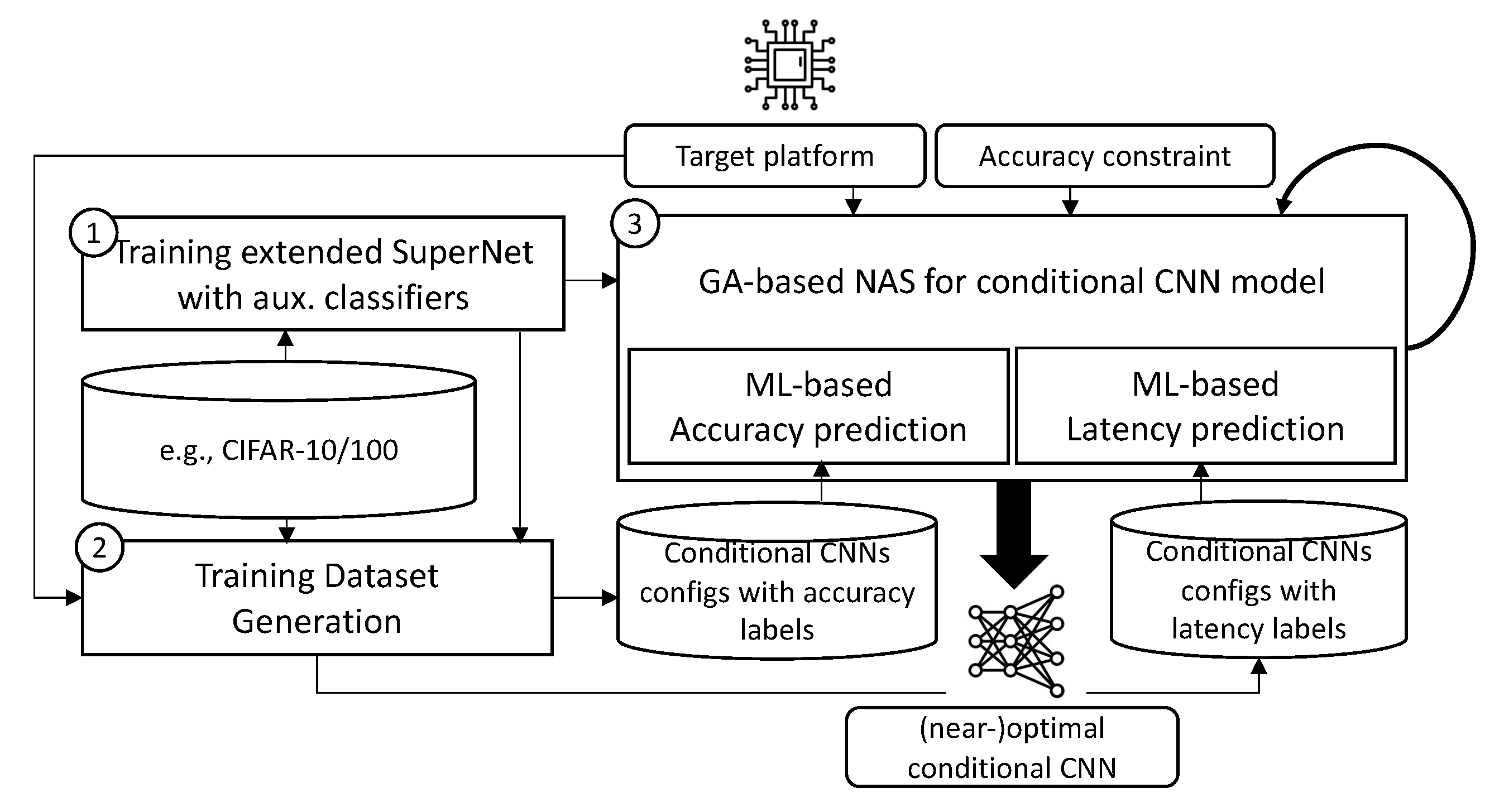
Figure 1 shows the overall structure of CondNAS and its design flow. Similar to OFA, the SuperNet is first trained independent of target platforms (①), then the GA is later performed for the given target platform. The SuperNet is extended such that it can incorporate the various configurations of auxiliary classifiers. The GA in CondNAS adopts machine learning-based accuracy and latency prediction models to evaluate the score of an arbitrary conditional CNN encountered in the search. To this end, before the GA starts, the training dataset generation module extracts a number of various conditional CNNs from the SuperNet and generates their accuracy and latency label for the given target platform (②) in a similar way to BPNet: it actually runs and profiles the conditional CNNs, feeding the calibration dataset. The generated datasets are used for training the prediction models, which are then used in the search of (near-)optimal conditional CNNs for the given target platform (③). The SuperNet and the accuracy prediction model are trained only once for a new input image dataset, whereas the latency prediction model should be trained whenever the target platform changes.
3.2. Extending SuperNet
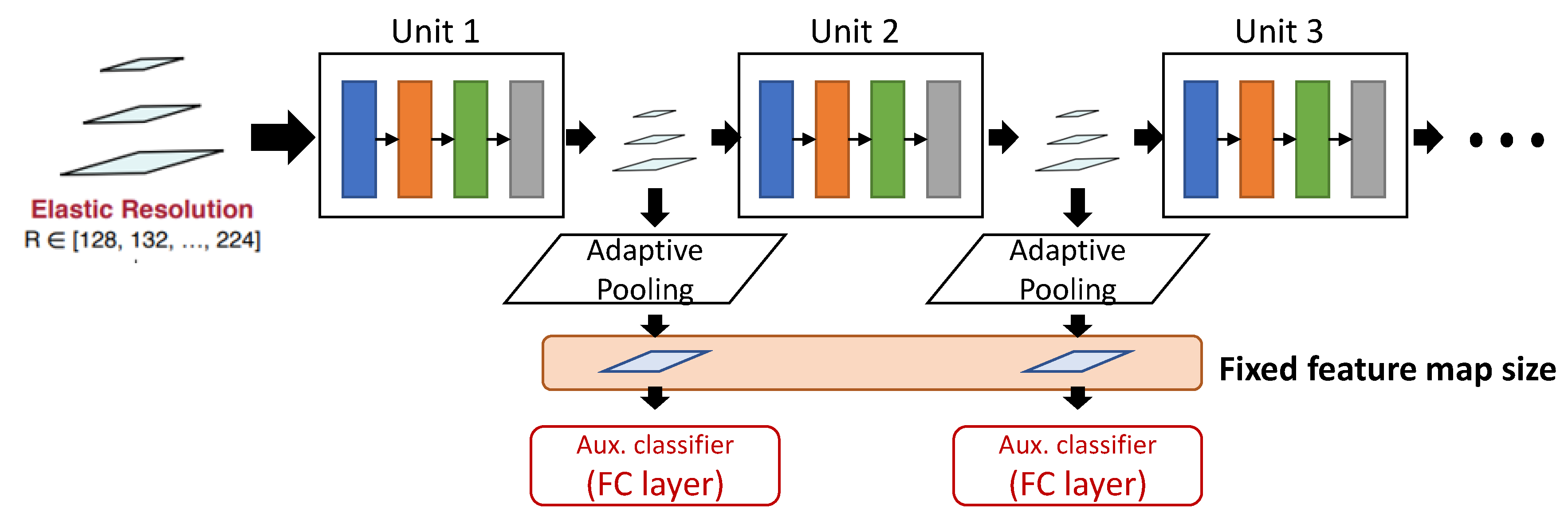
The first challenge for integrating OFA with BPNet is where to attach the auxiliary classifiers. In BPNet, the initial candidate locations of auxiliary classifiers are after every convolution layer. Although this has a potential to lead to more efficient conditional CNNs, it would make SuperNet training difficult or infeasible because a unit has a varying number of convolution layers: having a different number of auxiliary classifiers in a unit will make the loss function complicated. On the other hand, if we allow an auxiliary classifier to be attached only at the end of each unit, then the loss function of a unit will have the same number (i.e., one) of auxiliary classifiers and, hence, SuperNet training would be more tractable.
The second challenge for integrating OFA with BPNet is how to attach the auxiliary classifiers. SuperNet can take multiple input sizes and the auxiliary classifier attached to the SuperNet should be able to. As the auxiliary classifiers are fully connected layers, they are dependent on the size of input feature maps, unlike convolution layers. To address this problem, we propose to add an adaptive pooling layer before an auxiliary classifier so that the different sized input feature maps can be converted to a fixed size input feature map, as shown in Figure 2. While conventional pooling layers determine the output feature map size using stride and padding parameters, adaptive pooling layers compress the feature maps into a fixed size feature map. However, this can incur accuracy loss as average pooling layers in the proposed SuperNet convert the feature maps based on the minimal input image size. This minimizes the overhead of auxiliary classifiers in the inference and makes the training of the SuperNet with auxiliary classifiers more tractable: when the actual input size is larger than the minimal size, the information loss occurs. Although the information loss can lead to the accuracy loss, the reduced information can also play the role of a regularizer and prevent overfitting, actually increasing the overall accuracy. We examine the impact of average pooling on the overall accuracy.
3.3. Chromosome Design
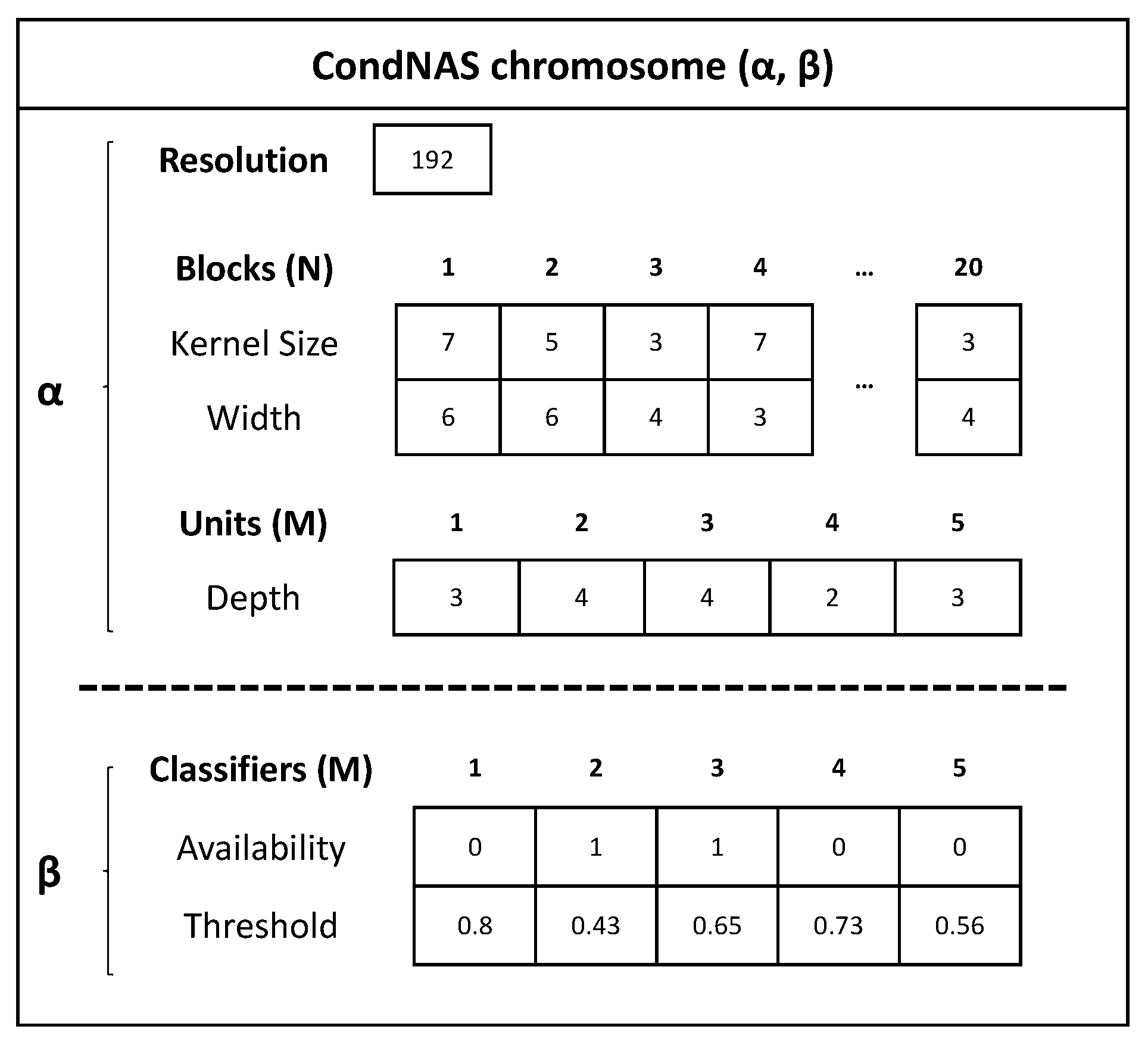
Once a SuperNet with auxiliary classifiers is trained by progressive shrinking, GA searches for the optimal conditional CNN for the target platform. Figure 3 shows the chromosome used in CondNAS’s GA module. The base CNN architecture () is encoded in three parts: image resolution, Blocks (N), and Units (M). A base CNN has five units, each of which has from two to four blocks (i.e., depth is at least two and the maximum number of blocks in the entire network is 20), and a block has two genes for kernel size and width, respectively. Thus, is encoded in 1 + 20 × 2 + 5 = 46 genes. On the other hand, conditional CNN architecture () encodes the availability and threshold of each auxiliary classifier after each of five units, resulting in 5 × 2 = 10 genes.
3.4. Accuracy Prediction of Conditional CNN
Performance estimation is a key factor that enables efficient and accurate design space exploration in GA. If performance estimation is not accurate, GA would not evolve correctly and fail to find the (near-)optimal solutions. If performance estimation is not efficient, it would be too time-consuming to explore sufficiently large design space. To this end, OFA proposed an accuracy predictor of a CNN. In BPNet, however, the accuracy of a conditional CNN was not estimated but was directly measured using a calibration dataset and the profiled information was used in GA. However, such a direct profiling would be infeasible in CondNAS due to significantly larger design space. In BPNet, the calibration dataset consists of 10,000 images, and the profiling time to measure softmax values at the auxiliary classifiers of an conditional CNN is about 1–2 min. The number of conditional CNN architectures in GA of CondNAS is 50,000 as a population of 100 individuals is evolved through 500 generations. Thus, the total time for directly calculating the accuracy of the conditional CNNs in CondNAS’s GA would be 50,000 × 1–2 min = 833–1666 GPU h, or 35–70 GPU days, which corresponds to 9–18 days even with a server having four GPUs. If the target platform is changed, or the GA should be re-run with different parameters, the whole process must be repeated, consuming another 833–1666 GPU h. One might consider reusing the profiled softmax values because the accuracy of conditional CNNs is independent of target platforms. However, it is highly likely that the individuals (i.e., the newly generated arbitrary conditional CNN architectures) from the GA are new and cannot be reused, considering the significantly large design space: .
To mitigate this problem, we devise an accuracy predictor to predict the accuracy instead of directly measuring the softmax values of the calibration dataset and calculating the accuracy of a conditional CNN. The accuracy predictor is already provided in OFA, but it is for conventional CNNs, not for conditional CNNs. The accuracy prediction of a conditional CNN is challenging but OFA has shown that it is feasible for conventional CNNs: multi-layer perceptron (MLP) takes a CNN of interest as input and very accurately predicts its accuracy. They achieved 0.21%p root mean square error (RMSE). It was reported that 1000–2000 training data (i.e., CNNs with accuracy labels) were used. For the prediction of conditional CNN accuracy, we devised a prediction model and empirically found that 200 training data for a base CNN (i.e., different locations and threshold values of auxiliary classifiers in a given base CNN, with accuracy labels) are sufficient to achieve a good accuracy of 0.4%p RMSE. The training dataset generation for the proposed accuracy prediction model of conditional CNNs is performed in two steps: it first constructs the softmax LUT for each of 2000 base CNNs using 10 K calibration dataset in a similar manner to BPNet. Then, the accuracy values of 200 different configurations of auxiliary classifiers were calculated using the LUT and stored as training data. Thus, the training generation time is 2000 × 60 + 2000 × 200 × 0.1 s ≅ 44 h, when the softmax profiling for one takes 1 min and the accuracy calculation and store for one pair of (, ) takes 0.1 s when is fixed.
The accuracy prediction model is trained with the generated training dataset consisting of 400 K arbitrary conditional CNNs. In OFA, the CNN accuracy prediction model is an MLP consisting of three layers. To predict the accuracy of a conditional CNN, which is much more complicated due to auxiliary classifiers, MLP may not be sufficient. Recently, gradient boosting-based ensemble decision tree models, such as XGBoost [20] and LightGBM [21], have been proposed, showing high performance in classification and regression problems. In particular, LightGBM can mitigate the drawbacks of XGBoost, such as long training time and being easy-to-overfit. In addition, it can be accelerated using CUDA, further reducing the training time. In this work, we use LightGBM rather than MLP to predict the accuracy of conditional CNNs. Note that, once the accuracy prediction model is trained, it is reused in CondNAS’s GA no matter how many times the target platform is changed.
3.5. Latency Prediction of Conditional CNN
A CNN latency is dependent on the target platform and a conditional CNN latency is further dependent on the input image because it allows early exit at the auxiliary classifier. OFA and BPNet both use LUT-based latency estimation. In OFA, the execution time of different types of layers with various shapes is profiled in advance on the target platform and stored in an LUT, which is then referenced by the latency estimator in the GA to estimate the latency of an arbitrary CNN. Because a CNN layer latency is almost the same regardless of input images, the latency estimator references the LUT and simply adds the latency of each layer in the CNN. In BPNet, the base CNN is fixed and the latency as well as the softmax value at each branch (i.e., auxiliary classifier) in the conditional CNN is profiled and stored in an LUT in advance; then, it is looked up in the GA (i.e., branch pruning stage). However, CondNAS cannot construct the latency LUT of the conditional CNNs in advance as the base CNN is not fixed but is arbitrary, unlike BPNet. Similarly, OFA’s approach of adding the layer latency to estimate the entire network latency is not efficient because, unlike OFA, CondNAS should estimate the conditional CNN latency for all input images as it varies depending on input images. Thus, it must run all input images in the calibration dataset to obtain the mean latency of the conditional CNNs, whereas OFA’s latency estimator for (base) CNNs need only one calculation to estimate the latency as it does not vary depending on the input image. Therefore, we also propose to predict the latency of conditional CNNs with the LightGBM model. Similarly to the accuracy prediction model, the latency prediction model is trained with a number of diverse conditional CNNs with latency labels. Then, it can efficiently predict the mean latency of a given conditional CNN without running any input images during GA. The similar order of time is required for the latency training dataset generation as the accuracy dataset. Unlike the accuracy training dataset, the latency training dataset cannot be reused when the target platform is changed.
4. Evaluations
The base SuperNet used in this study was from OFA, whose building block is based on MobileNet-v3 [22]. To compare with the results in BPNet, CIFAR-10 and CIRAR-100 datasets were used to fine-tune the SuperNet. As the image size of SuperNet is 224 × 224 while the size in CIFAR-10 and CIFAR-100 is 40 × 40, upsampling was completed as a pre-processing step before training.
To train the extended SuperNet, PyTorch 1.5.1 was used with Horovod [23] for the distributed deep learning across two nodes, one with four Titan V GPUs and the other with two Titan RTX GPUs. The GA algorithm used was NSGA-III [24]. The inference was made using TensorFlow Lite 2.3 on Galaxy Note10+, where the GPU is Mali-G76 and the CPU consists of two Mongoose M4 cores, two Cortex-A75 cores, and four Cortex-A55 cores.
4.1. Training of SuperNet for Conditional CNNs
4.1.1. Accuracy Comparison
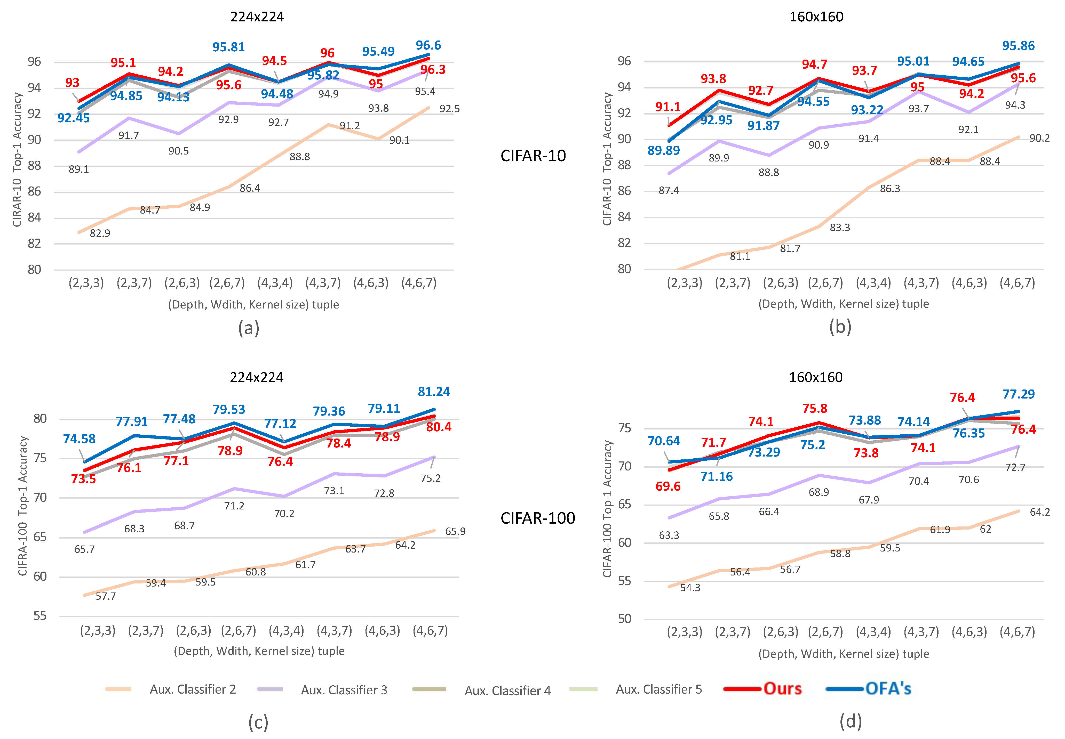
Figure 4 shows the test accuracy of the original SuperNet from OFA and the proposed extended SuperNet with auxiliary classifiers when depth (i.e., number of layers in a unit), width (i.e., number of channels), and kernel size are varied. For CIFAR-10, the proposed SuperNet with auxiliary classifiers shows 0.2%p of very little accuracy loss compared to the original OFA SuperNet accuracy. For CIFAR-100, the accuracy loss is also as small as 0.8%p. The accuracy of the last two auxiliary classifiers (ID 4 and 5) show accuracies comparable to the final classifier, which indicates that the test data in CIFAR-10 and CIFAR-100 are sufficiently easy to classify, already at the point of the fourth auxiliary classifier. In contrast, the first auxiliary classifier shows very poor accuracy, based on which we do not consider attaching an auxiliary classifier after the first unit in the design space exploration.
We observed that our proposed SuperNet with auxiliary classifiers cannot be trained with the hyperparameters of OFA, suffering from overshooting. Thus, we gradually reduced the learning rate and empirically found the learning rate, which does not incur overshooting. Correspondingly, we increased the number of epochs in the first stage of progressive shrinking. The other hyperparameters from OFA were used unchanged. Hyperparameters for conditional CNNs, loss weight, , and coefficient, c, have been added. However, unlike BPNet, where c is in the range of 1.0 and 4.0, we fixed c to 1.0 as c > 1.0 results in overshooting in SuperNet training. For , the same value was used as in BPNet.
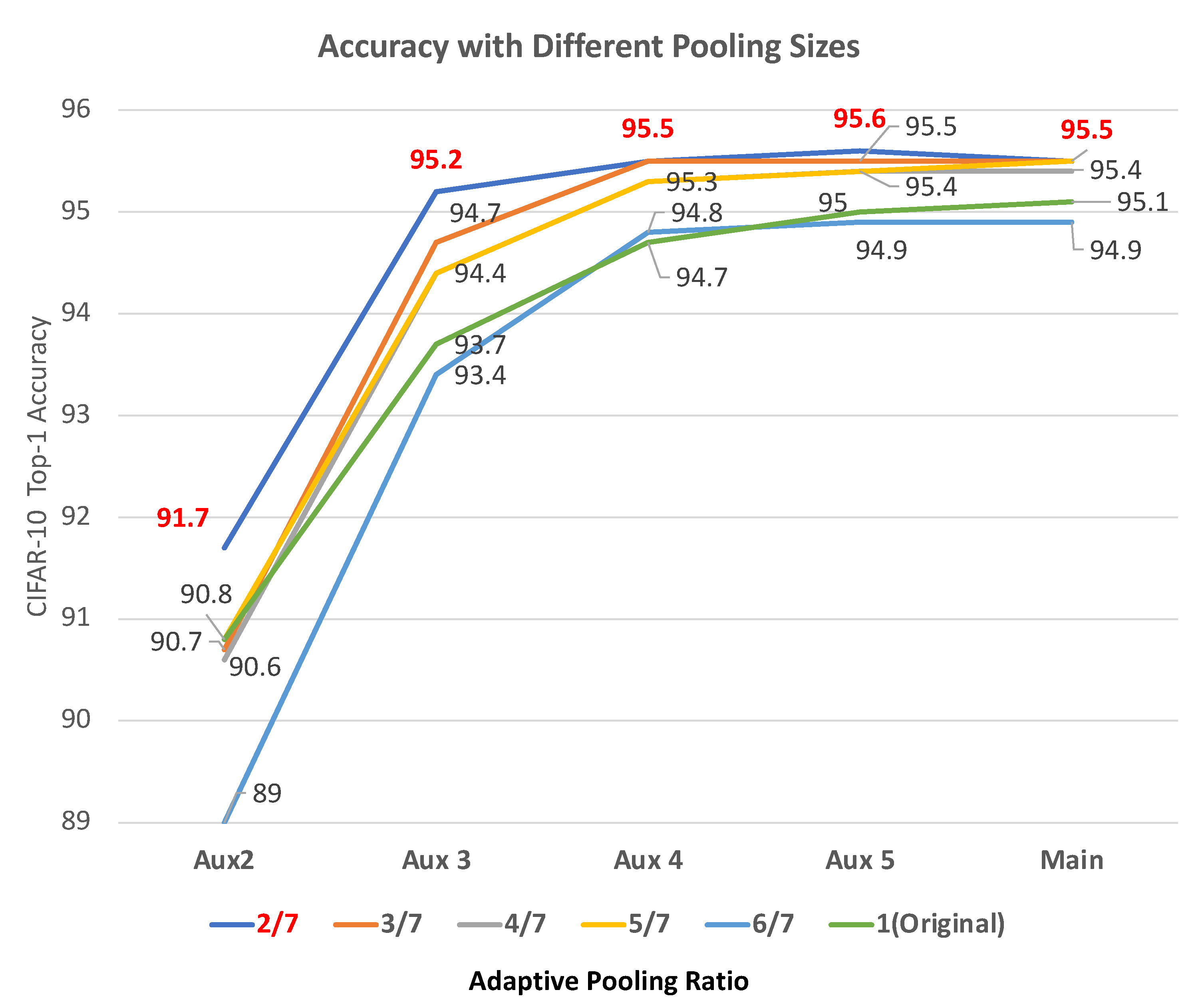
4.1.2. Effect of Adaptive Pooling
Figure 5 shows the accuracy when the adaptive pooling size is varied. The adaptive pooling size is defined to be the output of an adaptive pooling layer. In the proposed SuperNet, auxiliary classifiers are attached through an adaptive pooling layer so that the feature map size in the classifiers is fixed. Due to this, we expected a certain level of accuracy loss. As shown in Figure 5, however, most of the sizes except for one led to an increased accuracy by up to 2.17%p. Counter-intuitively, the smallest size, 64 × 64, shows the highest accuracy. It is because adaptive pooling normalizes largely distributed information, preventing overfitting. Note that, without adaptive pooling, we observe that the SuperNet with auxiliary classifiers cannot be trained.
4.2. Efficient Search in GA
4.2.1. Accuracy and Latency Prediction for Conditional CNNs
For accuracy and latency prediction of a conditional CNN, we devised light gradient boosting machine (LightGBM) models that take as input an arbitrary conditional CNN and predicts its accuracy and latency. The train dataset was generated as explained in Section 3. The number of for each was 200 while the number of was 3000, resulting in the total size of the train data being 600,000. To compare the accuracy of the proposed LightGBM model with the MLP model architecture from OFA, which consists of the three layers, they were trained with the same dataset of 600,000 arbitrary conditional CNNs for 2000 epochs. It took about 6.8 h for the MLP models, whereas LightGBM models took only about 40 s on a Titan RTX GPU.
Figure 6 shows the comparison results. For the accuracy prediction, the LightGBM model (Figure 6d) shows a significantly smaller RMSE of 0.15%p than the MLP model (Figure 6c), whose RMSE is 2.0%p. The proposed latency prediction model also shows accurate latency predictions with 0.75 ms of RMSE (Figure 6b) while the MLP model shows 1.5 ms of RMSE (Figure 6a).
4.2.2. Optimal Conditional CNNs
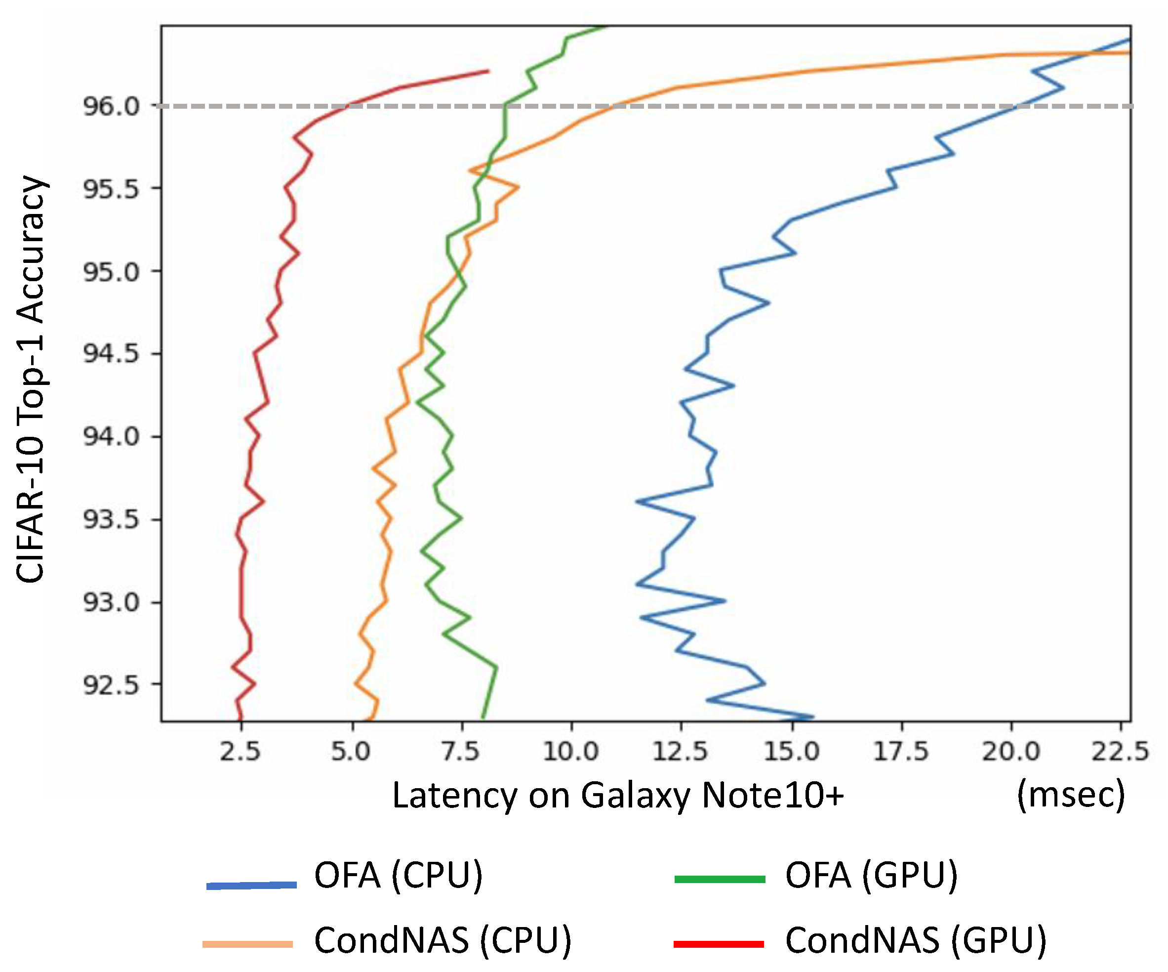
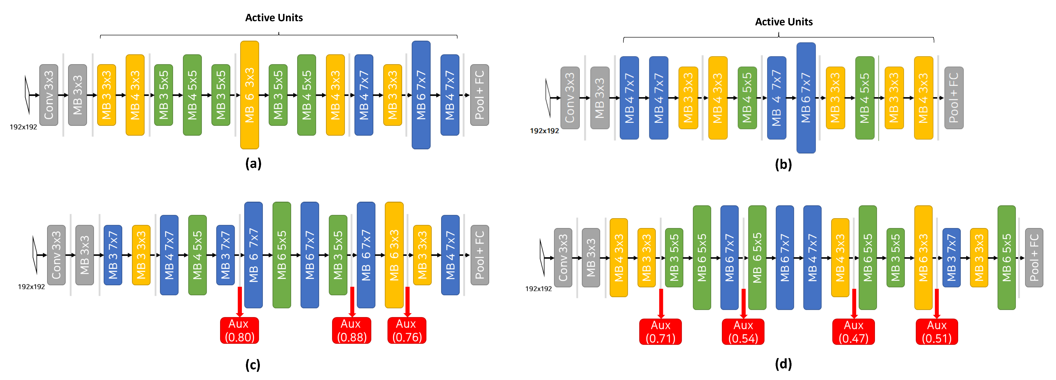
CondNAS can find a set of (near-)optimal conditional CNNs with shortest latency for the target platforms while meeting the accuracy constraint. Figure 7 shows the Pareto-optimal curves obtained by the prediction models in CondNAS and OFA for Galaxy Note10+ CPU and GPU. The accuracy of 0.96, which is smaller than the maximum accuracy by only 0.3%p, was selected as the comparison point because the conditional CNNs with higher accuracy tend to have only one auxiliary classifier at the end before the main classifier, with a large threshold: they are similar to the typical CNNs, having no advantage of the conditional architecture. For the same accuracy of 0.96, the conditional CNNs from CondNAS are 2.52× faster than the CNNs from OFA for the GPU (i.e., Mali-G76) and 1.75× faster for the CPU (i.e., mainly two Mongoose M4 cores). The large speedups come from the early exit in the conditional CNNs. As shown in Figure 8, the base CNNs are different from the those obtained by OFA, which confirms that CondNAS can successfully find (near-)optimal conditional CNNs, efficiently exploring the huge design space.
Figure 8 shows examples of (near-)optimal conditional CNNs obtained by CondNAS and CNNs by OFA. For the CPU, the CNN latency (Figure 8a) was 20.3 ms while the conditional CNN latency (Figure 8c) was 11.6 ms, achieving a 1.75× speedup. For the GPU, the CNN latency (Figure 8b) was 8.3 ms while the conditional CNN latency (Figure 8d) was only 3.3 ms, achieving a 2.52× speedup. All four CNNs had the same top-1 accuracy of 0.96: accuracy is not sacrificed in conditional CNNs. Note that the base CNN of conditional cases are different from the OFA CNNs, having different depth, width, and kernel sizes in each unit.
When the BPNet method was applied to the CNN obtained by OFA, the resultant conditional CNN could not maintain the accuracy of 0.96, but resulted in 0.925 with the latency of 14.98 ms. The conditional CNN obtained by CondNAS for the same accuracy of 0.925 showed 5.10 ms, achieving a 2.94× speedup.
5. Discussions
The conditional CNNs obtained from CondNAS can achieve significantly faster inference than the CNNs from OFA for the same platform, thanks to the auxiliary classifiers. However, the maximum accuracy in the conditional CNNs from CondNAS tends to be lower than the CNNs from OFA for the same reason: due to the early exist, an input image may not be thoroughly examined with all the layers in the network. Even if CondNAS carefully determined the threshold for the early exist in the auxiliary classifiers and the location of classifiers in a network, the maximum accuracy can be lower than that of the conventional CNNs without auxiliary classifiers. However, the difference is usually negligible, being less than 1%p. As the purpose of employing conditional CNNs is to reduce the latency while meeting the accuracy constraint, such a negligible difference in maximum accuracy should be acceptable. Nevertheless, one can try to reduce the maximum accuracy difference, for example, by further improving the accuracy prediction model for the conditional CNNs.
In this work, we examined the efficacy of CondNAS with CIFAR-10 and CIFAR-100. It remains as future work to examine it with a complex dataset such as ImageNet.
6. Conclusions
In this paper, we proposed an efficient NAS technique called CondNAS for conditional CNNs for the fast yet accurate inference on diverse target platforms. CondNAS integrates two prior works, OFA and BPNet, carefully taking into account how to extend SuperNet for the conditional CNNs and how to predict the accuracy and latency of an arbitrary conditional CNN to make GA efficient. By using adaptive pooling as a glue, the SuperNet with the auxiliary classifiers could be trained without accuracy loss. By using an efficient training dataset generation, the proposed accuracy and latency prediction model in LightGBM shows very accurate prediction results. The experimental results show that the conditional CNNs obtained from CondNAS for Galaxy Note10+ GPU (Mali-G76) is 2.52× faster than the CNN from OFA, and the conditional CNNs from CondNAS for Galaxy Note10+ CPU (mainly Mongoose M4) is 1.75× faster than the CNN from OFA. The conditional CNN obtained by simply applying BPNet to the CNN from OFA could not maintain the same top-1 accuracy and the latency was also 2.94× slower than the conditional CNN obtained from CondNAS.
Author Contributions
Conceptualization, Y.Y. and G.P.; Data curation, G.P.; Funding acquisition, Y.Y.; Investigation, Y.Y.; Methodology, G.P. and Y.Y.; Project administration, Y.Y.; Software, G.P.; Supervision, Y.Y.; Validation, G.P. and Y.Y.; Visualization, G.P.; Writing—original draft, G.P. and Y.Y. All authors have read and agreed to the published version of the manuscript.
Funding
This work was supported by the 2018 Research Fund of the University of Seoul.
Data Availability Statement
The data presented in this study are available on request from the corresponding author.
Conflicts of Interest
The authors declare no conflict of interest.
Abbreviations
The following abbreviations are used in this manuscript:
| CNN | Convolution neural network |
| NAS | Neural architecture search |
| GA | Genetic algorithm |
| OFA | Once-for-all |
| BPNet | Branch-pruned network |
| DSE | Design space exploration |
| MLP | Multi-layer perceptron |
| LUT | Lookup table |
| LightGBM | Light gradient boosting machine |
| RMSE | Root mean square error |
References
- Jacob, B.; Kligys, S.; Chen, B.; Zhu, M.; Tang, M.; Howard, A.; Adam, H.; Kalenichenko, D. Quantization and training of neural networks for efficient integer-arithmetic-only inference. In Proceedings of the IEEE Conference on Computer Vision and Pattern Recognition, Salt Lake City, UT, USA, 18–22 June 2018. [Google Scholar]
- Zhang, X.; Zhou, X.; Lin, M.; Sun, J. Shufflenet: An extremely efficient convolutional neural network for mobile devices. In Proceedings of the IEEE Conference on Computer Vision and Pattern Recognition, Salt Lake City, UT, USA, 18–22 June 2018. [Google Scholar]
- Iandola, F.N.; Song, H.; Moskewicz, M.W.; Ashraf, K.; Dally, W.J.; Keutzer, K. SqueezeNet: AlexNet-level accuracy with 50× fewer parameters and <0.5 MB model size. arXiv 2016, arXiv:1602.07360. [Google Scholar]
- Howard, A.G.; Zhu, M.; Chen, B.; Kalenichenko, D.; Wang, W.; Weyand, T.; Andreetto, M.; Adam, H. Mobilenets: Efficient convolutional neural networks for mobile vision applications. arXiv 2017, arXiv:1704.04861. [Google Scholar]
- Lavin, A.; Gray, S. Fast algorithms for convolutional neural networks. In Proceedings of the IEEE Conference on Computer Vision and Pattern Recognition, Las Vegas, NV, USA, 27–30 June 2016; pp. 4013–4021. [Google Scholar]
- Zoph, B.; Le, Q.V. Neural architecture search with reinforcement learning. arXiv 2016, arXiv:1611.01578. [Google Scholar]
- Zoph, B.; Vasudevan, V.; Shlens, J.; Le, Q.V. Learning transferable architectures for scalable image recognition. In Proceedings of the IEEE Conference on Computer Vision and Pattern Recognition, Salt Lake City, UT, USA, 18–22 June 2018. [Google Scholar]
- Pham, H.; Guan, M.Y.; Zoph, B.; Le, Q.V.; Dean, J. Efficient neural architecture search via parameter sharing. arXiv 2018, arXiv:1802.03268. [Google Scholar]
- Liu, H.; Simonyan, K.; Yang, Y. Darts: Differentiable architecture search. arXiv 2018, arXiv:1806.09055. [Google Scholar]
- Real, E.; Aggarwal, A.; Huang, Y.; Le, Q.V. Regularized evolution for image classifier architecture search. In Proceedings of the AAAI Conference on Artificial Intelligence, Honolulu, HI, USA, 27 January–1 February 2019. [Google Scholar]
- Tan, M.; Le, Q.V. Efficientnet: Rethinking model scaling for convolutional neural networks. arXiv 2019, arXiv:1905.11946. [Google Scholar]
- Tan, M.; Chen, B.; Pang, R.; Vasudevan, V.; Sandler, M.; Howard, A.; Le, Q.V. Mnasnet: Platform-aware neural architecture search for mobile. In Proceedings of the IEEE Conference on Computer Vision and Pattern Recognition, Long Beach, CA, USA, 15–20 June 2019. [Google Scholar]
- Wu, B.; Dai, X.; Zhang, P.; Wang, Y.; Sun, F.; Wu, Y.; Tian, Y.; Vajda, P.; Jia, Y.; Keutzer, K. Fbnet: Hardware-aware efficient convnet design via differentiable neural architecture search. In Proceedings of the IEEE Conference on Computer Vision and Pattern Recognition, Long Beach, CA, USA, 15–20 June 2019. [Google Scholar]
- Cai, H.; Zhu, L.; Han, S. Proxylessnas: Direct neural architecture search on target task and hardware. arXiv 2018, arXiv:1812.00332. [Google Scholar]
- Cai, H.; Gan, C.; Wang, T.; Zhang, Z.; Han, S. Once-for-all: Train one network and specialize it for efficient deployment. arXiv 2019, arXiv:1908.09791. [Google Scholar]
- Panda, P.; Sengupta, A.; Roy, K. Conditional deep learning for energy-efficient and enhanced pattern recognition. In Proceedings of the Design, Automation & Test in Europe Conference & Exhibition, Dresden, Germany, 14–18 March 2016. [Google Scholar]
- Jayakodi, N.K.; Chatterjee, A.; Choi, W.; Doppa, J.R.; Pande, P.P. Trading-off accuracy and energy of deep inference on embedded systems: A co-design approach. IEEE Trans. Comput. Aided Des. Integr. Circuits Syst. 2018, 37, 2881–2893. [Google Scholar] [CrossRef]
- Teerapittayanon, S.; McDanel, B.; Kung, H. Branchynet: Fast inference via early exiting from deep neural networks. In Proceedings of the 23rd International Conference on Pattern Recognition (ICPR), Cancun, Mexico, 4–8 December 2016. [Google Scholar]
- Park, K.; Oh, C.; Yi, Y. BPNet: Branch-pruned conditional neural network for systematic time-accuracy tradeoff. In Proceedings of the 57th ACM/IEEE Design Automation Conference (DAC), Virtual, 20–24 July 2020. [Google Scholar]
- Chen, T.; Guestrin, C. Xgboost: A scalable tree boosting system. In Proceedings of the 22nd ACM SIGKDD International Conference on Knowledge Discovery and Data Mining, San Francisco, CA, USA, 13–17 August 2016. [Google Scholar]
- Ke, G.; Meng, Q.; Finley, T.; Wang, T.; Chen, W.; Ma, W.; Ye, Q.; Liu, T. Lightgbm: A highly efficient gradient boosting decision tree. In Proceedings of the Advances in Neural Information Processing Systems 30 (NIPS 2017), Long Beach, CA, USA, 4–9 December 2017. [Google Scholar]
- Howard, A.; Sandler, M.; Chu, G.; Chen, L.; Chen, B.; Tan, M.; Wang, W.; Zhu, Y.; Pang, R.; Vasudevan, V.; et al. Searching for mobilenetv3. In Proceedings of the IEEE International Conference on Computer Vision, Seoul, Korea, 27–28 October 2019. [Google Scholar]
- Sergeev, A.; Balso, M.D. Horovod: Fast and easy distributed deep learning in TensorFlow. arXiv 2018, arXiv:1802.05799. [Google Scholar]
- Cui, Z.; Chang, Y.; Zhang, J.; Cai, X.; Zhang, W. Improved NSGA-III with selection-and-elimination operator. Swarm Evol. Comput. 2019, 49, 23–33. [Google Scholar] [CrossRef]
Figure 1.
CondNAS overall structure and design flow.

Figure 2.
Adaptive pooling as a glue to attach auxiliary classifiers to SuperNet.

Figure 3.
CondNAS chromosome with 56 genes.

Figure 4.
Accuracy comparison of SuperNets with (a) CIFAR-10 and image size of 224 × 224, (b) CIFAR-10 and 160 × 160, (c) CIFAR-100 and 224 × 224, and (d) CIFAR-100 and 160 × 160.
Figure 4.
Accuracy comparison of SuperNets with (a) CIFAR-10 and image size of 224 × 224, (b) CIFAR-10 and 160 × 160, (c) CIFAR-100 and 224 × 224, and (d) CIFAR-100 and 160 × 160.

Figure 5.
Accuracy when adaptive pooling size is varied. Original size is 224 × 224.

Figure 6.
Accuracy and latency prediction comparison: (a) MLP model for latency prediction, (b) LightGBM model for latency prediction in CondNAS, (c) MLP model for accuracy prediction in OFA, and (d) LightGBM model for accuracy prediction in CondNAS.
Figure 6.
Accuracy and latency prediction comparison: (a) MLP model for latency prediction, (b) LightGBM model for latency prediction in CondNAS, (c) MLP model for accuracy prediction in OFA, and (d) LightGBM model for accuracy prediction in CondNAS.

Figure 7.
Pareto optimal curves from OFA and CondNAS for CPU and GPU in Galaxy Note 10+, respectively.
Figure 7.
Pareto optimal curves from OFA and CondNAS for CPU and GPU in Galaxy Note 10+, respectively.

Figure 8.
Examples of (near-)optimal CNNs obtained from OFA for Galaxy Note10+ (a) CPU and (b) GPU, and examples of (near-)optimal conditional CNNs obtained from CondNAS for Galaxy Note10+ (c) CPU and (d) GPU.
Figure 8.
Examples of (near-)optimal CNNs obtained from OFA for Galaxy Note10+ (a) CPU and (b) GPU, and examples of (near-)optimal conditional CNNs obtained from CondNAS for Galaxy Note10+ (c) CPU and (d) GPU.

Publisher’s Note: MDPI stays neutral with regard to jurisdictional claims in published maps and institutional affiliations. |
© 2022 by the authors. Licensee MDPI, Basel, Switzerland. This article is an open access article distributed under the terms and conditions of the Creative Commons Attribution (CC BY) license (https://creativecommons.org/licenses/by/4.0/).
Share and Cite
MDPI and ACS Style
Park, G.; Yi, Y. CondNAS: Neural Architecture Search for Conditional CNNs. Electronics 2022, 11, 1101. https://doi.org/10.3390/electronics11071101
AMA Style
Park G, Yi Y. CondNAS: Neural Architecture Search for Conditional CNNs. Electronics. 2022; 11(7):1101. https://doi.org/10.3390/electronics11071101
Chicago/Turabian StylePark, Gunju, and Youngmin Yi. 2022. "CondNAS: Neural Architecture Search for Conditional CNNs" Electronics 11, no. 7: 1101. https://doi.org/10.3390/electronics11071101
Note that from the first issue of 2016, this journal uses article numbers instead of page numbers. See further details here.