Mathematical Formula Image Screening Based on Feature Correlation Enhancement

Abstract

There are mathematical formula images or other images in scientific and technical documents or on web pages, and mathematical formula images are classified as either containing only mathematical formulas or formulas interspersed with other elements, such as text and coordinate diagrams. To screen and collect images containing mathematical formulas for others to study or for further research, a model for screening images of mathematical formulas based on feature correlation enhancement is proposed. First, the Feature Correlation Enhancement (FCE) module was designed to improve the correlation degree of mathematical formula features and weaken other features. Then, the strip multi-scale pooling (SMP) module was designed to solve the problem of non-uniform image size, while enhancing the focus on horizontal formula features. Finally, the loss function was improved to balance the dataset. The accuracy of the experiment was 89.50%, which outperformed the existing model. Using the model to screen images enables the user to screen out images containing mathematical formulas. The screening of images containing mathematical formulas helps to speed up the creation of a database of mathematical formula images.

1. Introduction

Mathematical language is an international, universal language that is not restricted by regions or languages. The main form of mathematical language is mathematical formulas. Mathematical formulas are often the quintessence of technical documents. At present, there are a large number of images of mathematical formulas with research value in web pages or scientific and technological documents. However, they are also mixed with other images, and crawling the page image directly will result in obtaining all the images. If only images containing mathematical formulas need to be obtained, further screening is required.

The essence of mathematical formula image screening is to automatically classify a large number of images into two categories: images with mathematical formulas and images without mathematical formulas. Mathematical formula images can be further divided into two cases: mathematical formulas only and mathematical formulas interspersed between text or coordinate diagrams. The focus of mathematical formula image screening is how to categorize images of situations where formulas are interspersed with text, illustrations, and other elements as well as mathematical formula images.

Traditional image classification techniques [1] rely on the designer’s prior knowledge and cognitive understanding of the classification task, resulting in worse experimental performance. In recent years, convolutional neural networks have performed prominently in image feature learning [2,3,4,5]. Convolutional neural networks extract features through autonomous learning, effectively circumventing the many drawbacks arising from complex feature extraction. LeCun et al. [6] proposed the LeNet-5 network to introduce convolutional neural networks into the field of image classification for the first time [7]. The LeNet-5 network achieved a classification error rate of 0.8% in the classification task of handwritten digit image recognition, and achieved excellent classification results, confirming the superiority of convolutional neural networks in image classification. However, due to the lack of large-scale training data, limited by the theoretical basis and computer computing power, the recognition effect of LeNet-5 for complex images is not ideal [8]. Since then, various network models have been proposed for classification tasks. Xie et al. [9] proposed ResNeXt, a highly modular network architecture for image classification. ResNeXt is a combination of ResNet [10] and Inception [11]. Unlike Inception v4 [12], the ResNeXt structure does not require the complex design of the Inception structure, adopting the same topology for each branch. Zhang et al. [13] proposed a modular architecture ResNeSt. ResNeSt applies channel attention to different network branches, succeeding in cross-feature interaction. Furthermore, attention mechanisms [14,15,16] are also introduced into image classification tasks. The attention mechanism focuses on important information with high weight, ignores irrelevant information with low weight, and learn independently, and can continuously adjust the weight. Hu et al. [17] proposed a SENet module that focuses on channel features, and which obtains different weights by learning the relationship between channels. Li et al. [18] proposed a dynamic selection mechanism for convolution kernels, SKNet. SKNet allows each neuron to adaptively adjust the size of its convolution kernel according to the multi-scale of the input information. Different from SENet, SKNet not only considers the weights between channels, but it also considers the weights of different convolutions in each branch, which is equivalent to incorporating a soft attention mechanism [19].

Existing feature processing methods and image classification models enhance feature extraction and classification capabilities. However, since the mathematical formula image may contain elements such as text and coordinate diagrams, it is difficult for the existing classification models to meet the classification requirements of the task in this paper. In view of the fact that convolutional neural networks can extract deep features, and the attention mechanism can focus on the information that needs attention in the task, this paper proposes a mathematical formula image screening model based on feature correlation enhancement. The aim is to use the model to screen and collect images containing mathematical formulas for further study. Aiming at the problem that irrelevant features may affect model classification accuracy, a feature correlation enhancement (FCE) module has been designed. First, the FCE module uses a soft attention mechanism to obtain features with channel weights and convolution kernel weights. Then, the features with high weight information are fused into the feature self-attention process, so that the self-attention can strengthen the internal correlation between the mathematical formula features and weaken the contribution of other features in the subsequent stage. Aiming at the problem of image size and the characteristics of the horizontal writing of formulas, a strip multi-scale pooling (SMP) module has been designed. The SMP module integrates strip pooling into the spatial pyramid pooling so that the horizontal writing mathematical formula features get more attention, and can unify the feature dimension, eliminating the constraint that the convolutional neural network needs a fixed-size input. The experimental results of the AttNeSt model have been compared with those of other models, and the results show the superior performance of the AttNeSt model. Using the trained model to screen the test images resulted in screening out most of the images containing mathematical formulas.

The main contributions of this paper are as follows:

• For the influence of irrelevant features on the model, a feature correlation enhancement module (FCE) has been designed. FCE enhances the internal correlation of mathematical formula features through the interaction of soft attention and self-attention to reduce the influence of other features on the classification decisions.
• Aiming at the problem of inconsistent image size and the characteristic of horizontal writing in formulas, a strip multi-scale pooling (SMP) module was designed. SMP solves the size constraint by integrating spatial pyramid pooling (SPP) [20] into the network, and then extracting rectangular horizontal features using a strip pooling module (SPM) [21] to increase the attention of the horizontal structure.
• To solve the problem of unbalanced datasets, this paper introduces regularization into the binary cross-entropy loss function [22]. By cascading regularization, the improved loss function distributes the weights equally to different image features, which avoids the fitting phenomenon and speeds up the model convergence.

The remainder of the paper is structured as follows: the Section 2 illustrates a mathematical formulation image screening method based on feature correlation enhancement; the Section 3 analyzes and discusses the experimental results, and the Section 4 summarizes the paper.

2. Materials and Methods

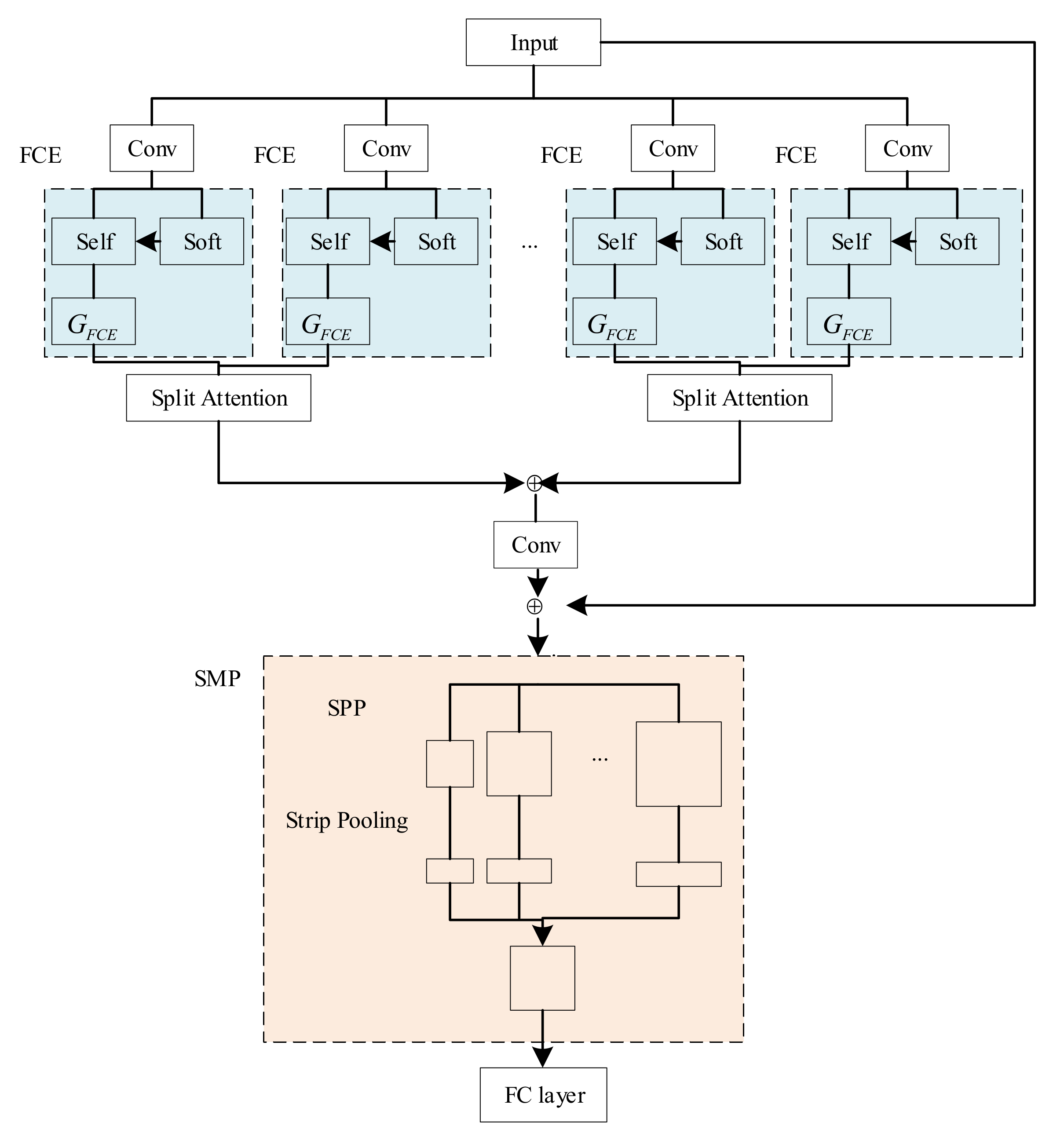
When designing the network, ResNeSt-50 [13] was used as the basic framework of the network to ensure that detailed information could be extracted. Compared with ResNet-50 [23], the essence of the improvement of ResNeSt-50 is the introduction of the split-attention module, which captures the relationship across channels through a channel-based attention mechanism. ResNeSt has achieved excellent results in image classification, object detection, instance segmentation, and semantic segmentation tasks. The network structure of the mathematical formula image screening model (AttNeSt) based on feature correlation enhancement is shown in Figure 1. In the figure, “Self” represents the self-attention mechanism, and “Soft” denotes the soft attention mechanism. AttNeSt replaces the second layer of convolution in the split-attention module with an FCE structure to strengthen the interaction and correlation of feature information in mathematical formulas and reduce the contribution of useless information. The SMP module is introduced after extracting features. The main idea is to add a set of horizontal stripe pooling to strengthen horizontal features after multi-scale pooling and before feature fusion.

2.1. Feature Correlation Enhancement (FCE) Module

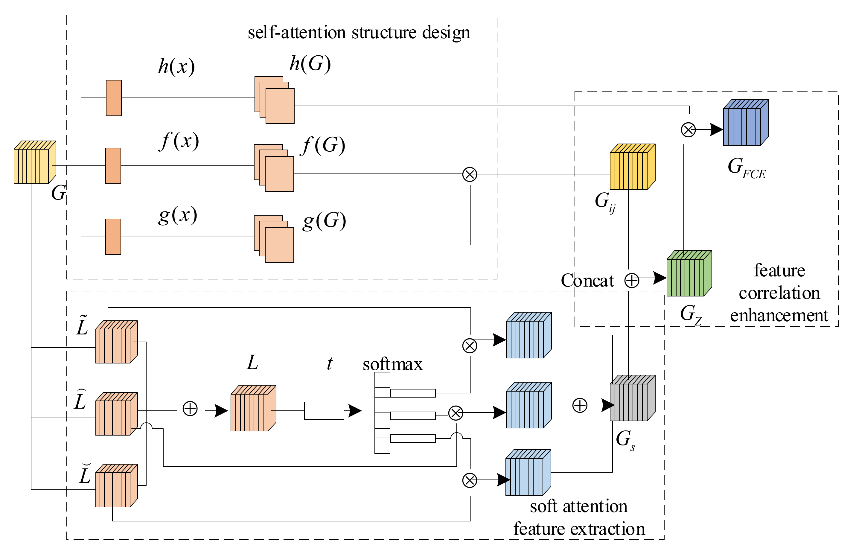
The convolution operation can process the features in the local receptive field but cannot correlate the global information to establish long-distance dependencies. The self-attention mechanism [24] can capture global information and obtain larger receptive-field and contextual information. SKNet [18] uses the convolution kernel attention to cause the network to adaptively adjust the size of the receptive field according to the multiple scales of the input information and obtain features with weight information. The feature correlation enhancement (FCE) module weights the feature weight information into the self-attention to increase the degree of association of the self-attention to the mathematical formula features, thus emphasizing the relevance and global dependency of such features and reducing the influence of other features on the classification. The feature correlation enhancement structure is shown in Figure 2, which is mainly divided into three parts, self-attention structure design, soft attention feature extraction, and feature correlation enhancement.

2.1.1. Self-Attention Structure Design

The self-attention mechanism aims to pay attention to some details according to the target object. The core is how to determine the parts that need attention based on the target, and to further analyze after finding the details. In this subsection, the process of the first stage of self-attention is described.

First, use the feature space mapping functions $f\left(x\right)=W_{f}x$, $g\left(x\right)=W_{g}x$ and $h\left(x\right)=W_{h}x$ to transform $G\in R^{C\times N}$ into three feature spaces $f\left(G\right)$, $g\left(G\right)$ and $h\left(G\right),$ where $N=H\times W$ represents the number of pixels. Then, perform matrix multiplication and normalization on $f\left(G\right)$ and $f\left(G\right)$ to obtain $G_{ij}$, as shown in Equation (1), where $a_{ij}=f{(G)}^{T}g\left(G\right)$ and $G_{ij}$ represents the degree of association between the $i$th dimension element in $f\left(G\right)$ and the $j$th dimension element in $g\left(G\right)$:

$$G_{ij}=\frac{\exp (a_{ij})}{{\sum }_{i=1}^N\exp (a_{ij})}$$

(1)

2.1.2. Soft Attention Feature Extraction

First, the feature map $X\in R^{H\times W\times C}$ is converted with convolution kernel sizes of 3, 5, and 7 to obtain 3 types of feature information from differnt convolutional kernels, $\tilde{L}$, $\stackrel{͡}{L}$, and $\breve{L}$, respectively, and summed to obtain $L$. Then, global average pooling (GAP) [25] is used to encode the convolutional layer $L$ to get $t$, $t\in R^C$, and a compression calculation is performed in the $H\times W$ dimension of $L$ to obtain the $c$th element $t_c$ in $t$, as shown in Equation (2). Finally, the weight information of different spatial scales $t=\left(t_1, t_2, \dots , t_C\right)$ is obtained:

$$t_c=F_{gp}(L)=\frac{1}{H\times W}{\displaystyle \sum }_{i=1}^H{\displaystyle \sum }_{j=1}^{W}L\left(i,j\right)$$

(2)

Use the softmax function for $t$ to obtain $a$, $b$, and $p$. $a$, $b$, and $p$ denote the soft attention channel weights of $\tilde{L}$, $\stackrel{͡}{L}$ and $\breve{L}$, respectively, as shown in Equation (3). $a_c$ denotes the $c$th element of $a$. The same is true for $b_c$ and $p_c$:

$$a_c=\frac{e^{A_{c}t}}{e^{A_{c}t}+e^{B_{c}t}+e^{P_{c}t}}, b_c=\frac{e^{B_{c}t}}{e^{A_{c}t}+e^{B_{c}t}+e^{P_{c}t}}, p_c=\frac{e^{P_{c}t}}{e^{A_{c}t}+e^{B_{c}t}+e^{P_{c}t}}$$

(3)

$A, B, \mathrm{and} P\in R^{C\times d}$, and $A_c\in R1\times d$ denote the $c$th row of $A$, and the same is true for $B_c$ and $P_c$. $d=\max (C/r, K)$, $r$ denotes the shrinkage rate, $K$ denotes the minimum value of $d$. Due to the different image sizes, GAP is used instead of the FC layer, with the advantage of reducing the number of parameters and receiving features of different scales.

The channel weights are multiplied by the feature information of different convolution kernels to obtain the feature vector $V$, as shown in Equation (4). $V$ fuses the information of multiple receptive fields and increases the weight of the mathematical formula features. $V$ is transformed into a feature map $G_s$ after ReLU activation and 3 × 3 convolution:

$$V=a·\tilde{L}+b·\stackrel{͡}{L}+p·\breve{L}$$

(4)

2.1.3. Feature Correlation Enhancement

The correlation between $f\left(G\right)$ and $g\left(G\right)$ is established in the first stage of self-attention, and the process is to give attention to the elements with high similarity through elemental interactions. Feature correlation enhancement is the second stage of self-attention. First, $G_{ij}$ is fused with the soft attention feature map $G_s$ with weight information to obtain $G_Z$. $G_Z$ is the self-attention feature map with channel weights and convolution kernel weights. Then, the contribution of the convolution kernel and channel weights to the mathematical formulation features is enhanced by calculating the degree of correlation between $G_Z$ and $h\left(G\right)$. The following is the specific calculation procedure.

The Concat [26] feature fusion mechanism splices two or more feature maps by channel or dimension. For the task of this paper, splicing on the channel dimension can better express the channel weights of soft attention features. The splicing on the channel dimension can better express the channel weights of the soft attention features, which in turn enables more feature representations of the mathematical formula feature maps in the self-attention features and strengthens the contribution of such features. Concat feature fusion requires equal feature map width and height. In this paper, we solve this problem by upsampling to obtain feature maps $G_s$ and $G_{ij}$ with the same $H$ and $W$.

Assuming that the number of channels of feature maps $G_s$ and $G_{ij}$ are $G_{1s}, G_{2s}, G_{3s, }\dots G_{cs}$ and $G_{1ij}, G_{2ij}, G_{3ij,} \dots G_{cij}$, respectively, denote the number of channels of feature $G_s$ by $C_s$, denote the number of channels of feature $G_{ij}$ by $C_{ij}$, and $1c$ denotes the tensor of $1\times 1\times c$. The output channel $Z_{Concat}$ is obtained after the Concat operation, as shown in Equation (5). At this point, the number of channels in the feature map becomes $C_s+C_{ij}$, and the feature map is denoted as $G_Z$:

$$Z_{Concat}={\displaystyle \sum }_{c=1}^{C_s}{X}_c·1c+{\displaystyle \sum }_{c=1}^{C_{ij}}{Y}_c·1c$$

(5)

The matrix multiplication operation is performed between $G_Z$ and $h\left(G\right)$, and then 1 × 1 convolution is performed to obtain the correlation-enhanced self-attention feature map $G_{FCE}$, as shown in Equation (6):

$$G_{FCE}={\displaystyle \sum }_{i=1}^N{G}_{Z}h\left(G_4\right)$$

(6)

2.2. Strip Multi-Scale Pooling (SMP) Module

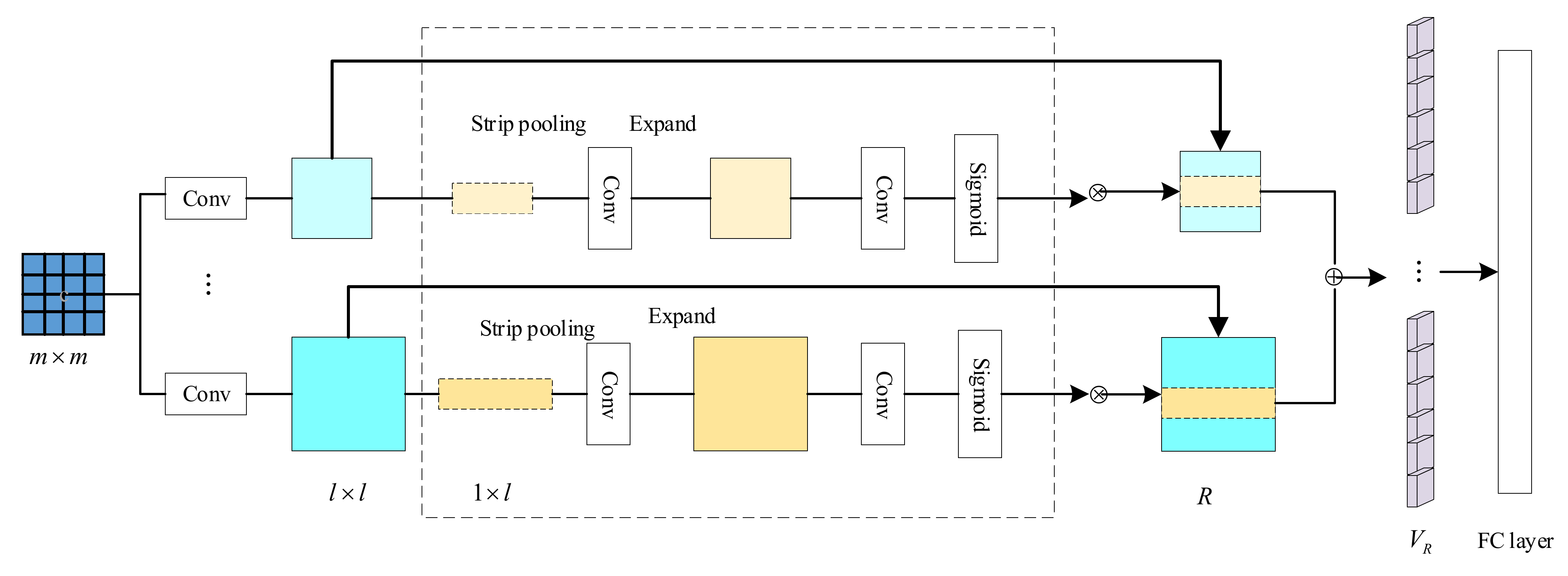
Spatial pyramid pooling [20] proposes a multi-scale pooling structure to unify the feature dimensions of different inputs, which is widely used in the field of image classification. Strip pooling [21] proposes a strategy that considers a long but narrow kernel, allowing the network to efficiently model long-range dependencies, focusing on horizontal or vertical features. Considering that the formula part of the mathematical formula image is written horizontally, this paper is inspired by SPP and SPM to design the SMP module. SMP can focus on horizontal information under the premise of unified feature dimension, increase the feature expression ability of mathematical formula, and then improve the classification accuracy. The structure is shown in Figure 3. (To simplify the image, only two pooling scales are shown in the figure).

In the process of unifying feature dimensions, the size of the pooling kernel varies according to the size of the input image. The pooling kernel (Filter) and step (Stride) are shown in Equations (7) and (8), where Filter is rounded up, and Stride is rounded down.

$$Filter=\left[m/l\right]$$

(7)

$$Stride=\left[m/l\right]$$

(8)

An example of a Level 3 SPP is shown in

Table 1. Example of three-level SPP parameters.

Input Size	Filter	Stride	Output Size	Output Length
10 × 10	10	10	1 × 1	35
	4	3	3 × 3
	2	2	5 × 5
15 × 15	15	15	1 × 1	35
	5	5	3 × 3
	3	3	5 × 5

.

The input size in Table 1 indicates the size of the feature map input to the SPP structure, corresponding to m × m in Figure 3, and the output size indicates the desired output size, corresponding to l × l in Figure 3. With the three-level SPP structure, two feature maps of different sizes obtain the same length output. If the input size changes, the pooling kernel and step size will also change to ensure that the output has the same length. Taking the input size 10 × 10 as an example, the feature map is subjected to three pooling operations with convolution kernels of 10, 4, and 2 and step sizes of 10, 3, and 2 to obtain the outputs of 1 × 1, 3 × 3, and 5 × 5, respectively. Similarly, the 15 × 15 feature map uses different convolution kernels and step sizes to obtain 1 × 1, 3 × 3, and 5 × 5 outputs.

After obtaining the feature map of multi-scale pooling, then strip pooling is performed. The realization process of horizontal strip pooling is shown in the dotted box in Figure 3. First, the $l\times l$-scale feature map is transformed into $1\times l$-scale features after horizontal strip pooling. The implementation is to calculate the average pixel value on the horizontal feature map corresponding to the pooling kernel, as shown in Equation (9), where $x\in R^{H\times W}$:

$$y_i^H=\frac{1}{l}{\displaystyle \sum }_{0\le j\le W}{x}_{i,j}$$

(9)

Then, the convolution operation with a convolution kernel size of Filter is used to expand along the top and bottom, and the expanded feature map is the same size as the original feature map. After the 1 × 1 convolution operation and Sigmoid activation, the feature map $R$ is obtained by multiplying with the corresponding pixels of the original feature map. The feature map $R$ is fused into a feature vector $V_R$. Images of all sizes are unified into a fixed dimension in $V_R$ and input into the fully connected layer.

The horizontal strip pooling considers the horizontal range rather than the whole feature map, reinforcing the information about the position of the formulas written horizontally in the feature map. Since the weights of the target features (mathematical formula features) have been increased during feature extraction, SMP pays more attention to the horizontal formula features and less attention to the text, which is also a horizontal feature.

2.3. Loss Function

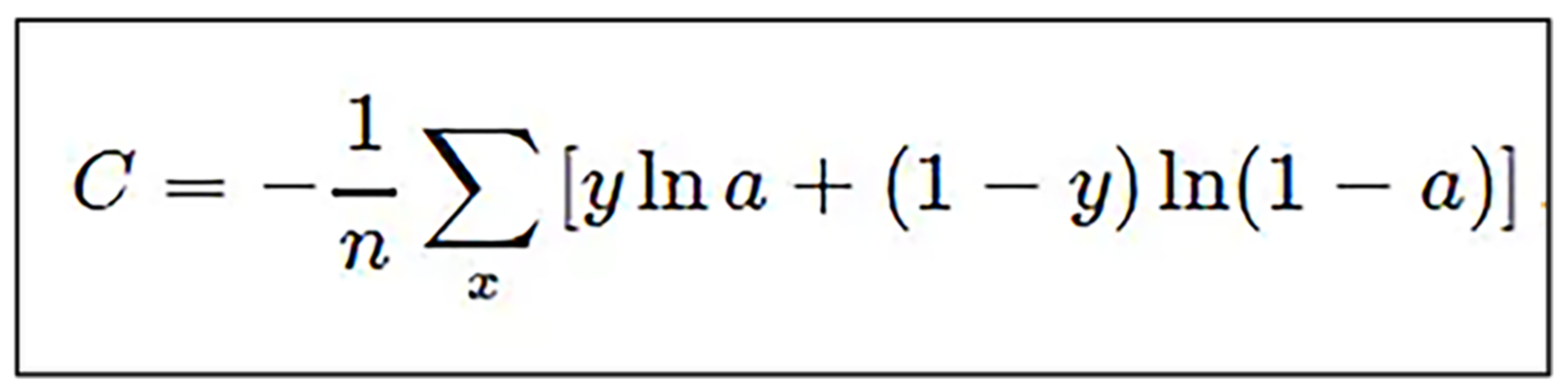
The images in the dataset in this paper are randomly crawled from the network, and the images are in various forms. To balance the dataset and improve the model accuracy and generalization performance, this paper improves the binary cross-entropy loss function (BC). The binary cross-entropy loss function formula is shown in Equation (10), where N denotes the total number of samples, y denotes the label of sample i, and p_i denotes the probability of sample i being predicted as category 1:

$$L_{org}=\frac{1}{N}{\displaystyle \sum }_i-\left[y_i\cdot log(p_i)+\left(1-y_i\right)\cdot log(1-p_i)\right]$$

(10)

Incorporating regularization in BC [27,28]. The L₁ and L₂ regularization [29,30] are shown in Equations (11) and (12), where $\beta$ is the regulating factor between the loss function and the regularization term, $n$ is the number of samples in the training set of the model, and $\delta$ is the weight parameter of the model:

$$L_{org1}=L_{org}+\frac{\beta }{n}{\displaystyle \sum }_{\delta }\left|\delta \right|$$

(11)

$$L_{org2}=L_{org}+\frac{\beta }{2n}{\displaystyle \sum }_{\delta }{\delta }^2$$

(12)

When only L₁ regularization is used, the same penalty is given to all weight parameters. When only L₂ regularization is used, a large penalty is given to parameters with larger weight parameters, and a small penalty is given to parameters with smaller weights. The improved binary cross-entropy loss function (IBC) is shown in Equation (13).

$$L_{new}=L_{org}+tp{\Vert \delta \Vert }_1+t\left(1-p\right){\Vert \delta \Vert }_2^2$$

(13)

$\left|\delta \right|$ is the absolute value of the weight parameter, ${\Vert \delta \Vert }_1$ is the 1NF of the weight parameter $\delta$, ${\Vert \delta \Vert }_2^2$ is the square of the 2NF of the weight parameter $\delta$, $t$ is the adjustment factor between the loss function and the L₂ regularization, $p$ is the adjustment factor between L₁ regularization and L₂ regularization, which degenerates to L₂ regularization if $p=0$ and to L₁ regularization if $p=1$. L₁ regularization is to extract one of the features randomly and drop the other features. L₂ regularization is the mean selection when the image features present a Gaussian distribution. Therefore, in IBC, L₁ regularization is introduced for feature selection, and then L₂ regularization is introduced to deal with the image features of covariance, and the weights are equally divided among various image features through a cascade of regularization to retain useful features.

3. Results and Discussion

3.1. Experimental Details on Image Classification

This section describes the experimental dataset and other experimental details.

3.1.1. Dataset and Data Augmentation

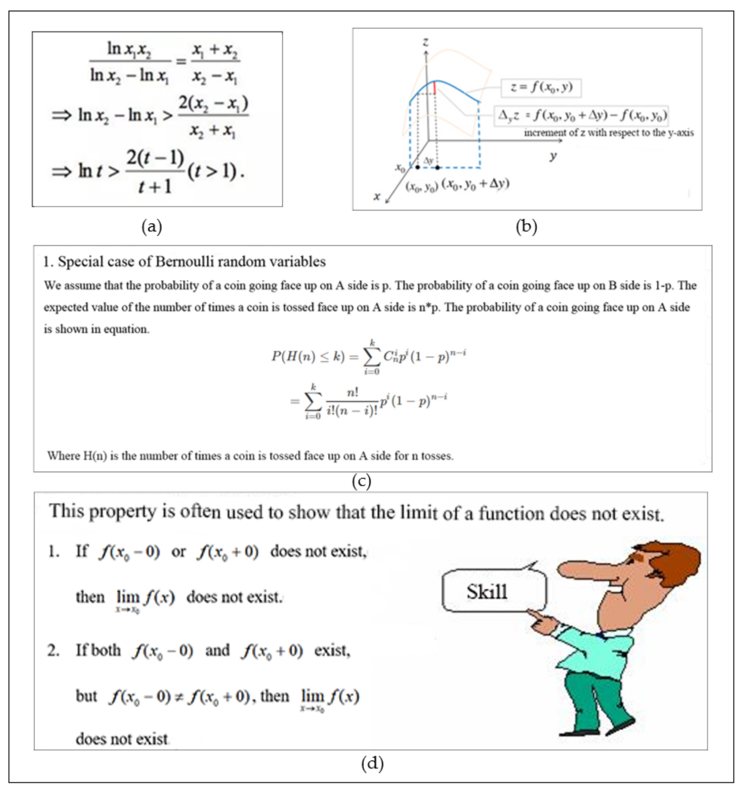
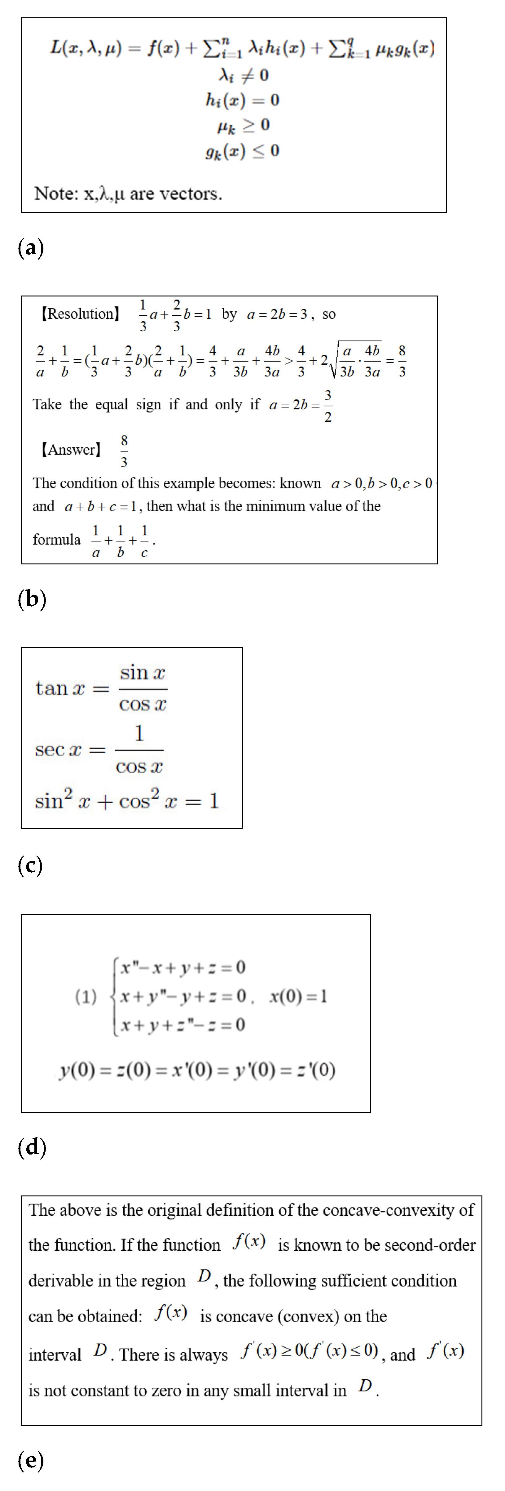
The public dataset im2latex-100k [31] collects a large number of mathematical expressions rendered in the real world, but the images of this dataset contain only mathematical formulas (e.g., Figure 4a) and not other elements (e.g., text, coordinate diagrams, illustrations, etc., in Figure 4b–d). If using im2latex-100k as the dataset leads to overfitting of the model, the model will only be able to distinguish images of the type shown in Figure 4a. Since there is no image dataset containing images such as Figure 4b–d, a homemade dataset is used as the object of processing in this paper. Images are randomly crawled from web pages or scientific and technical documents and manually pre-classified into two categories, one for images containing elements of mathematical formulas (category 1) and one for images not containing elements of mathematical formulas (category 0). The experiment takes 6250 of these images, 3125 images per class, of which 2188 images are used for the training set and 937 images for the validation set. Due to the small sample of images in this paper [32,33,34], a data enhancement strategy [35,36] was used to avoid overfitting during the training process. Specifically, the training set was enhanced to 21,880 images (10,940 images each for class 0 and class 1) using a 40-degree random rotation and horizontal flip operation, and the original size of the images was retained.

3.1.2. Training Strategy

The experimental hardware environment is an AMD Ryzen 5 2600 Hexa-core processor, 24 GB of RAM, and an Nvidia GeForce GTX 1660 Ti GPU. The software environment is tensorflow-gpu1.14 and keras2.2.5 deep learning framework. The optimizer is Adam. The number of iterations is 200 epochs, the batch size is 64, the learning rate is 0.001, β1 = 0.9, β2 = 0.999, epsilon = 1 × 10⁻⁸. The loss function is IBC, where the parameters $t=0.71$, $p=0.53$, and $\beta =0.81$. $K=32$ in the shrinkage rate $r$.

3.1.3. Evaluation Indicators

To comprehensively evaluate the classification performance of the model, Precision, Recall, F1-score, the amount of image data (Support), and Accuracy were used as evaluation indicators. The training time (Time (step/s)) was used as a measure of time complexity.

The formula is as follows, where (True Positive) is the correct prediction for category 1, (False Positive) is the prediction of category 0 to category 1, (False Negative) is the prediction of category 1 to category 0, and (True Negative) is the correct prediction of category 0.

Precision: The calculation is shown in Equation (14). $P1$ indicates the proportion of predicted category 1 examples to the actual category 1, and $P0$ indicates the proportion of predicted category 0 images to the actual category 0:

$$P1=TP/\left(TP+FP\right), P0=TN/\left(TN+FN\right)$$

(14)

Recall: The calculation is shown in Equation (15). $R1$ indicates the proportion of examples correctly predicted to be category 1 to all actual category 1 examples, and $R0$ indicates the proportion of examples correctly predicted to be category 0 to all actual category 0 examples:

$$R1=TP/\left(TP+FN\right), R0=TN/\left(FP+TN\right)$$

(15)

F1-score: The calculation is shown in Equation (16). $F1\_1$ denotes the harmonic mean of $P1$ and $R1$, and $F1\_0$ denotes the harmonic mean of $P0$ and $R0$:

$$F1\_1=2·\frac{P1·R1}{\left(P1+R1\right)}, F1\_0=2·\frac{P0·R0}{\left(P0+R0\right)}$$

(16)

Support: The number of images categorized into a certain category.

Accuracy (ACC): The calculation is shown in Equation (17), indicating the proportion of correctly predicted examples in all examples:

$$ACC=\frac{\left(TP+TN\right)}{\left(TP+FP+FN+TN\right)}$$

(17)

3.2. Experimental Results and Analysis

In this section, the experimental results of the image screening method (AttNeSt) are shown and compared with the experimental results of other methods.

3.2.1. Experimental Results of the AttNeSt Model

The AttNeSt model was trained following the experimental setup in Section 2.1.3. The experimental results are shown in

Table 2. Experimental results of AttNeSt.

Epoch	P0%	P1%	R0%	R1%	F1_0%	F1_1%	Support (0, 1)		ACC%
10	65.37	75.54	72.43	68.53	68.72	71.86	9894	11,986	70.12
20	68.41	86.73	83.22	73.55	75.09	79.60	8984	12,896	77.45
50	79.14	86.26	85.06	82.21	81.99	84.19	9963	11,917	82.32
100	84.56	90.45	89.52	86.48	86.97	88.42	10,044	11,836	87.43
150	86.37	90.96	88.77	87.99	87.55	89.45	10,487	11,393	89.41
200	87.42	91.38	90.02	88.16	88.70	89.74	10,560	11,320	89.50

.

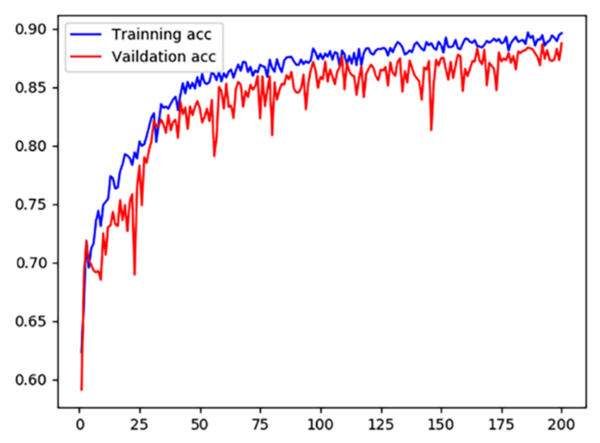
When the number of iterations is small, it is known from Support that the image imbalance is severe. As the number of iterations increased, all indicators improved. The experiment tried to continue the training after 200 iterations, the loss value tended to be constant, and the ACC no longer improved. To reduce the training time and overhead, the experiment set the maximum number of iterations to 200 epochs. The ACC variation is shown in Figure 5.

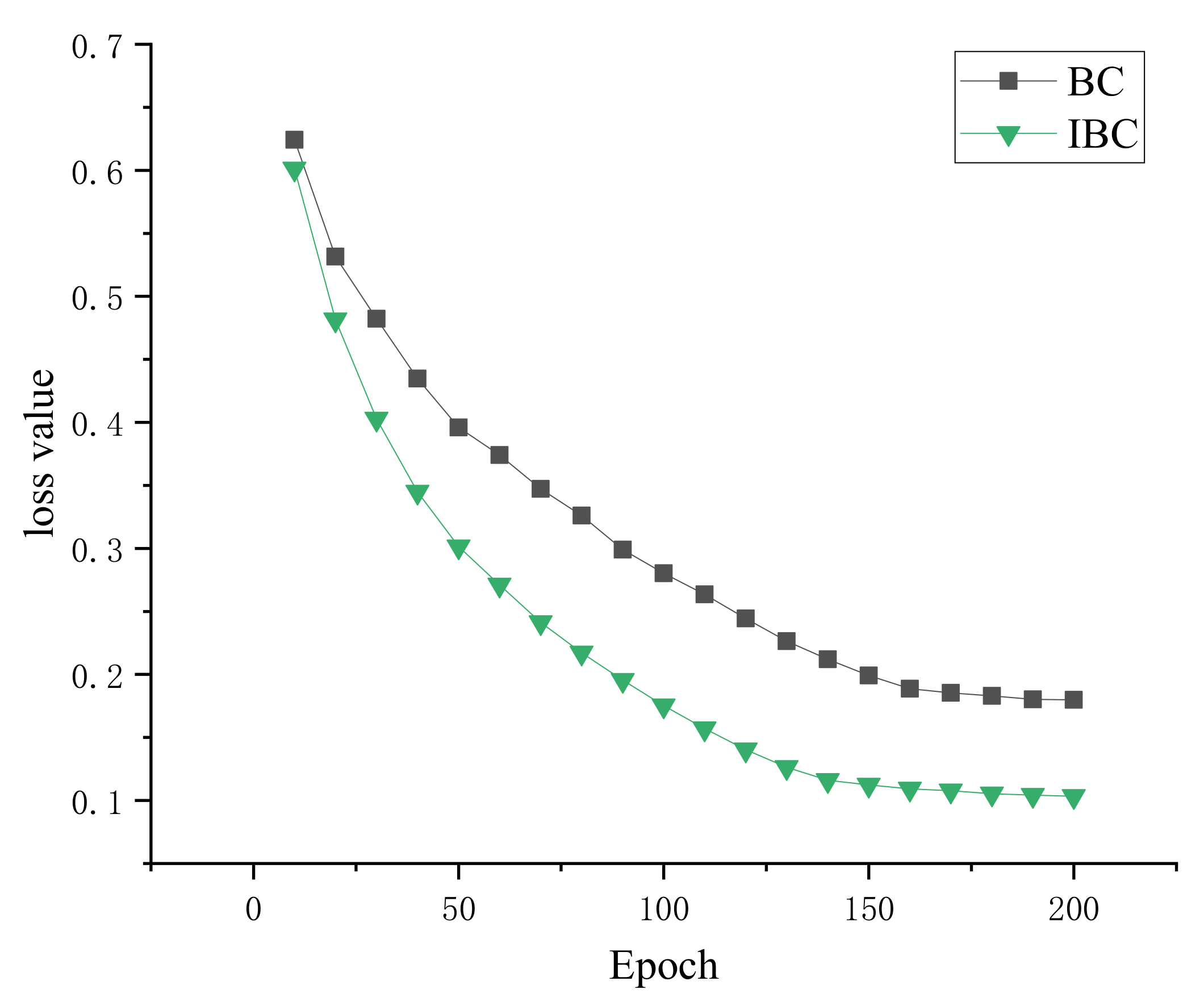
To verify whether IBC has an optimization effect on the model, the model was trained using BC while keeping other parameters consistent. When the model was trained using BC, the ACC was 87.73%, a decrease of 1.77% compared to when using IBC. The variation of loss values is shown in Figure 6. IBC converges faster and has lower loss values than BC. It can be proved that IBC has an optimization effect on the model.

3.2.2. Effect of SMP Structure on Results

Setting multiple pooling scales to explore the effect of SMP structure on classification performance:

• SMP_1: 1 × 1, 3 × 3, 5 × 5,
• SMP_2: 1 × 1, 5 × 5, 7 × 7,
• SMP_3: 1 × 1, 3 × 3, 7 × 7, 9 × 9,
• SMP_4: 1 × 1, 3 × 3, 7 × 7, 9 × 9, 11 × 11,
• SMP_5: 1 × 1, 3 × 3, 7 × 7, 9 × 9, 11 × 11, 13 × 13,
• Cropping: random cropping of images to 256 × 256 size,
• Warping: uniform image size of 256 × 256.

The experimental results are shown in

Table 3. Effect of pooling method on results.

Method	F1_0%	F1_1%	Support (0, 1)		ACC%	Time (Step/s)
SMP_1	78.54	81.27	9675	12,205	80.52	4.410
SMP_2	80.32	82.53	9905	11,975	81.78	4.423
SMP_3	88.70	89.74	10,560	11,320	89.50	4.479
SMP_4	74.62	71.25	8769	13,111	70.41	5.012
SMP_5	60.62	70.74	7843	14,937	64.44	5.432
Cropping	79.41	77.21	8932	12,948	79.32	4.012
Warping	73.47	72.46	7864	14,016	73.04	3.982

.

As can be seen from Table 3, the SMP structure can help the model learn more horizontal information while unifying the feature dimensions. SMP_1, SMP_2, and SMP_3 improved in all evaluation indicators compared to Cropping and Warping. SMP_3 has the highest ACC of 89.50% and the best results, as the number of images in both categories tend to be balanced. It indicates that the added 9 × 9 pooling kernel is better adapted to large-size images. SMP_4 and SMP_5 add 11 × 11 and 13 × 13 pooling kernels, respectively, with much lower ACC and F1 values and extremely unbalanced Support data. The reason for analysis is that there is an upper limit to the image size, and by continuously increasing the pooling kernel scale, receptive fields that are too large will acquire useless information and greatly increase the computational effort, thus affecting the results.

To explore the effect of strip pooling on classification performance, the strip pooling was removed from SMP_3, and the SPP structure was retained. The experimental results are shown in

Table 4. Effect of strip pooling on results.

Method	ACC%	Support (0, 1)		Time (Step/s)
SMP_3	89.50	10,560	11,320	4.479
SPP	88.81	10,472	11,408	4.465

.

There is no structure of strip pooling in SPP; instead, the features are directly dimensionally unified after multi-scale pooling. Some horizontal information may be lost in this process, and the ACC dropped by 0.69% although the training time is shorter. SMP_3 adds horizontal strip pooling before unifying the feature dimensions, which enables the model to focus more on horizontal features, and improve the ACC.

3.2.3. Effect of FCE Structure on Results

To verify the effect of the FCE module on the experiment, the FCE module is modified. SA is used to ablate the soft-attention feature extraction stage in the FCE module and retain the self-attention mechanism. Soft is to ablate the self-attention mechanism and retain the soft-attention feature extraction in the FCE module. ResNeSt-50 is the original ResNeSt-50 network model, and the experimental results are shown in

Table 5. Effect of FCE module on results.

Method	F1_0%	F1_1%	Support (0, 1)		ACC%
SA	86.09	85.82	9983	11,897	85.94
Soft	87.05	86.84	10,012	11,868	86.49
ResNeSt-50	81.13	80.01	9424	12,456	82.32
AttNeSt	88.70	89.74	10,560	11,320	89.50

.

As can be seen from the table, AttNeSt compared to ResNeSt-50 increased the FCE module, ACC improved by 7.18%, F1 value also improved greatly, and the number of images in each category (Support) tended to balance. The ACC of SA and Soft is 3.62% and 4.17% improved over ResNeSt-50, respectively, and all other metrics have been optimized. The ACC of AttNeSt is improved by 3.56% and 3.01% compared to SA and Soft, respectively. Experimental results show that adding soft-attention feature extraction or self-attention mechanism alone can improve the ACC of the model. The experimental results show that adding soft-attention feature extraction or a self-attention mechanism alone can improve the ACC of the model, and the FCE module integrates them so that the soft attention feature weights have a significant effect on the emphasis of useful features in self-attention, which can focus on other similar features and ignore the influence of useless features as much as possible, and the ACC is further improved.

3.3. AttNeSt Compared with Other Algorithms

To verify the superiority of the AttNeSt model and the added modules, this section compares the experimental results with other models.

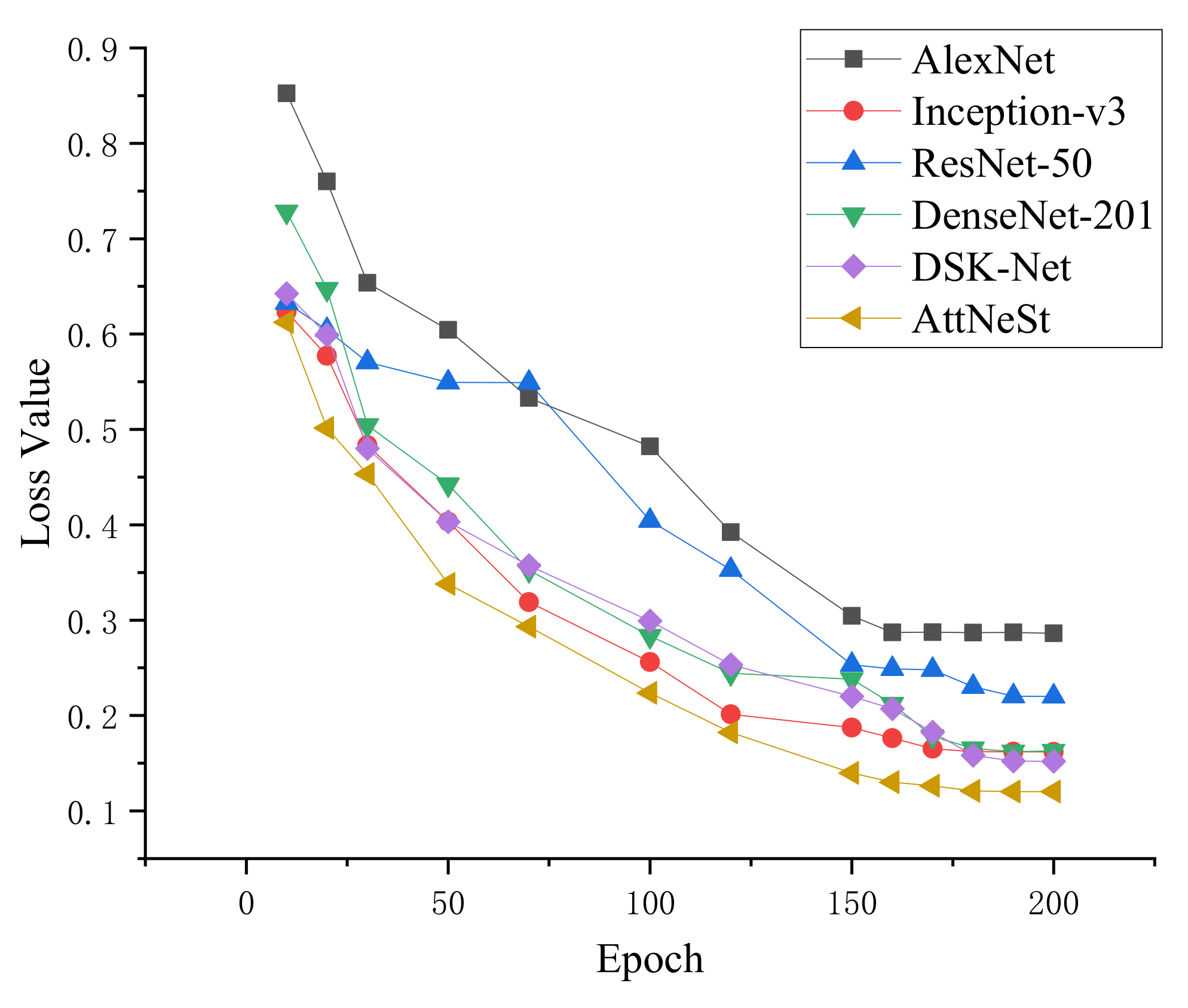
The purpose of the comparison experiments is to verify the performance of AttNeSt in the image screening task of mathematical formulas. The dataset and data augmentation are consistent with those in Section 3.1.1. This section compares the results of this paper’s algorithm with those of other algorithms for analysis. Other algorithms include AlexNet in the literature [37], Inception-v3 in the literature [38], ResNet-50 in the literature [23], DenseNet-201 in the literature [39], and DSK-Net in the literature [40]. All of the above network models add the SMP module before the fully connected layer so that the network model is not constrained by the image size. Softmax classification is added after the fully connected layer to output the probability that any image belongs to a certain class to suit our image classification task. The experimental results were determined with a learning rate of 0.001, an optimizer of Adam, a batch size of 64, and a loss function of IBC. The experimental results are shown in

Table 6. Results of comparison experiments.

Model	Support (0, 1)		ACC%	Time (Step/s)
AlexNet	8054	13,826	78.53	2.989
Inception-v3	9562	12,318	82.72	4.351
ResNet-50	9452	12,428	82.69	4.131
DenseNet-201	9354	12,526	84.57	4.272
DSK-Net	9876	12,004	83.54	4.292
AttNeSt	10,560	11,374	89.50	4.479

.

The results in Table 6 show that the ACC of AttNeSt is 10.97%, 6.78%, 6.81%, 4.93%, and 5.96% higher than that of AlexNet, Inception-v3, ResNet-50, DenseNet-201, and DSK-Net, respectively. The results showed that AttNeSt had a significant effect on ACC improvement and support for balance, and there was no significant increase in training time, within a manageable range.

The loss variation of each algorithm is shown in Figure 7. It can be seen from the figure that the AttNeSt has good convergence. The above experimental results show that the classification effect of the algorithm in this paper is better than those of other algorithms.

3.4. Mathematical Formula Image Screening Using AttNeSt Model

To verify the validity of the AttNeSt model, this section uses the trained AttNeSt network model to screen the images containing mathematical formulas.

3.4.1. Prediction for a Single Image

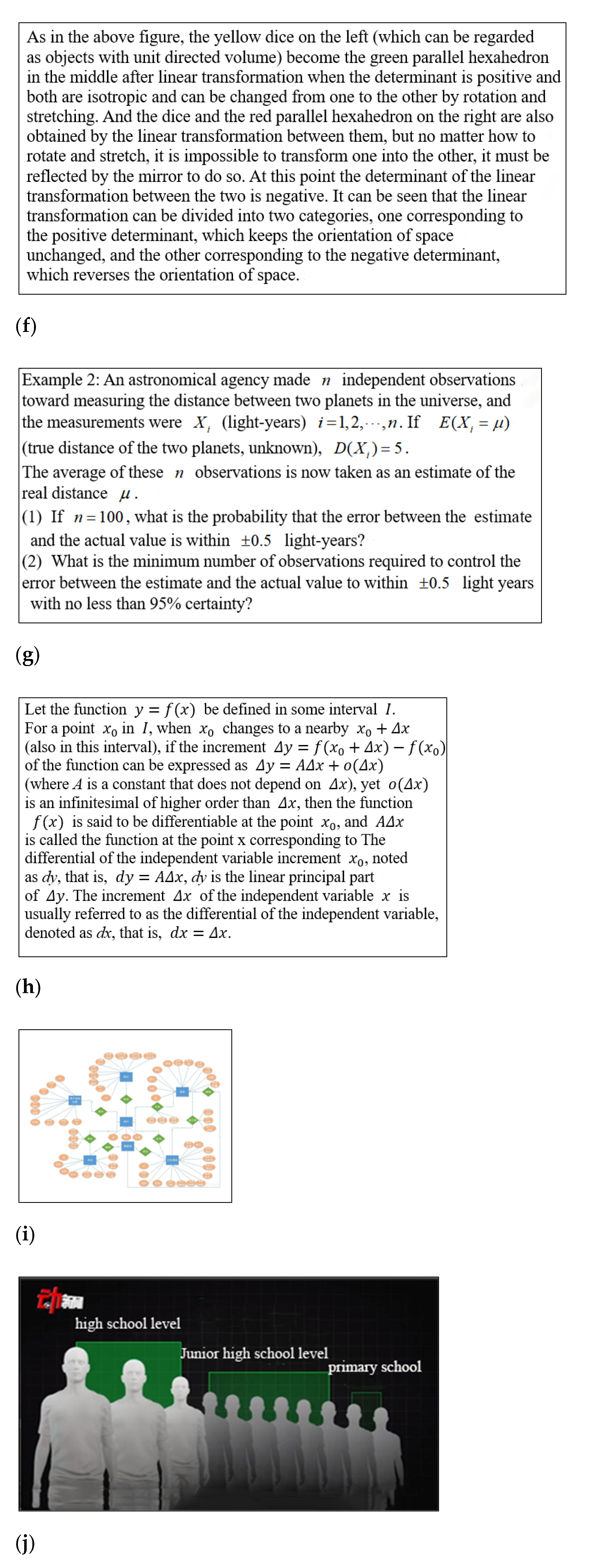
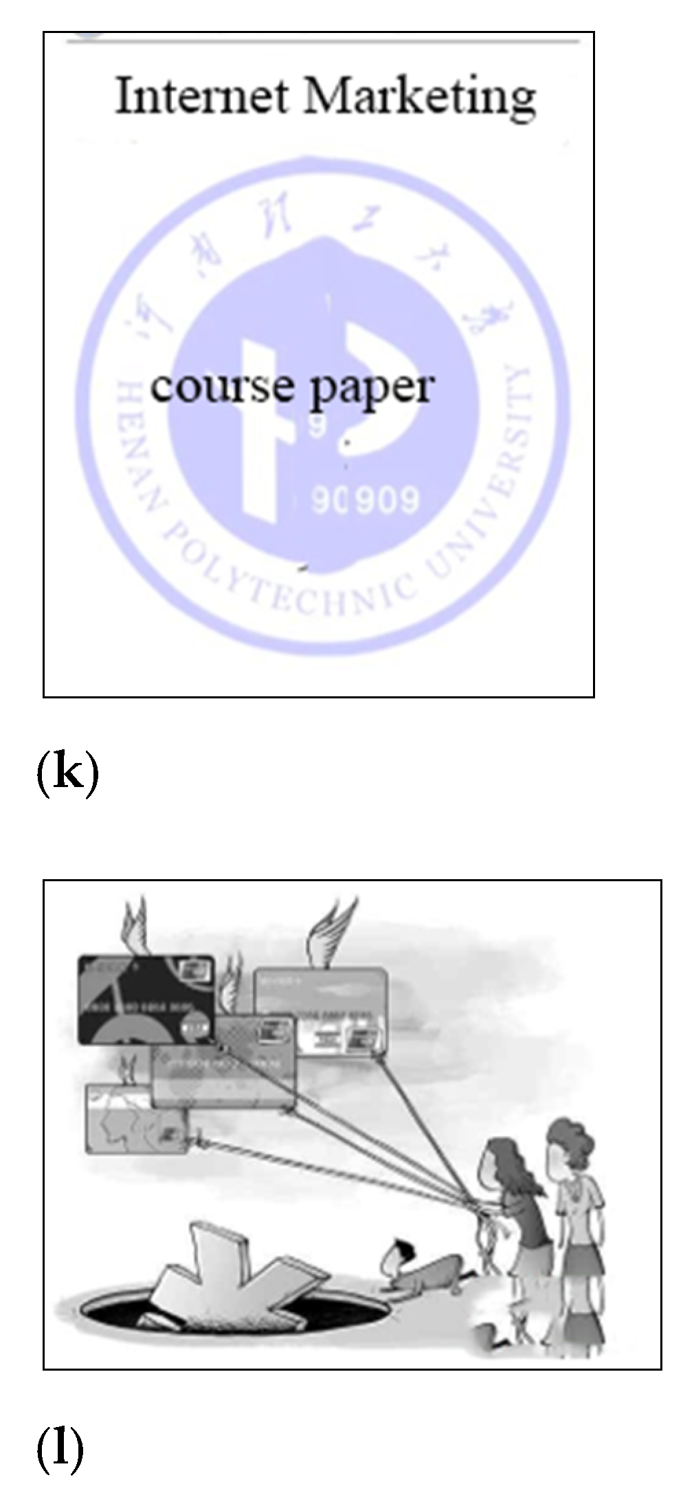
Twelve typical, original sample images crawled by the network are shown in Figure 8.The results of the classification of these 12 images using the trained AttNeSt are shown in

Table 7. Probability of image prediction.

Image	0	1
(a)	0.02561568	0.97438432
(b)	0.03445163	0.96554837
(c)	0.21873846	0.78126154
(d)	0.09284832	0.90715168
(e)	0.42943022	0.57056978
(f)	0.73022564	0.26977436
(g)	0.56458636	0.43541364
(h)	0.49839683	0.50160317
(i)	0.90454329	0.09545671
(j)	0.98567474	0.01432526
(k)	0.90865378	0.09134622
(l)	0.99678556	0.00321444

.

In this paper, we set out to classify the predicted images into a class with higher probability. From the data in Table 7, it can be seen that (a–d), (e), and (h) were assigned to category 1 and the rest were assigned to category 0. The effect was as expected.

3.4.2. Apply Other Models for Screening

Crawl all images on a web page or scientific document by keywords such as “math” or “formula” and tag each image with the category it belongs to. Take 2000 of these images, 1000 of which are of category 1, and 1000 of which are of category 0. Classification of images using the trained model in Section 3.3, the results are shown in

Table 8. Results of image category prediction.

Method	Correct (1)	Correct (0)	Mistake (1)	Mistake (0)	ACC%
AlexNet	711	691	309	289	70.10
Inception-v3	823	831	169	177	82.70
ResNet-50	767	811	189	233	78.90
DenseNet-201	815	854	146	185	83.45
DSK-Net	865	900	100	135	88.25
AttNeSt	921	967	33	79	94.40

, where Correct (1) indicates the number of images correctly assigned to category 1, Correct (0) indicates the number of images correctly assigned to category 0, Mistake (1) indicates the number of images belonging to category 0 but incorrectly assigned to category 1, and Mistake (0) indicates the number of images belonging to category 1 but incorrectly assigned to category 0.

As can be seen from Table 8, AttNeSt correctly classified 921 images to category 1, correctly classified 967 images to category 0, classified 33 images from category 0 to category 1, and classified 79 images from category 1 to category 0. Compared with the results of other models, AttNeSt screening is the best and can correctly classify most of the images containing mathematical formulas into category 1.

Due to the differences in images, the actual accuracy varies when using trained models for image classification. The error of AlexNet is larger because the results of AlexNet are not so good when the model is trained. The ACC when screening images using other trained models compared to the ACC when the models were trained (Table 6), the errors were within 5%.

3.4.3. Results of the im2latex-100k Dataset Screening

After observing the im2latex-100k dataset, all the images in it now have transparent backgrounds; such images cannot be processed in the AttNeSt network model, so the images must be processed into images with white backgrounds and black text, as shown in Figure 9:

The dataset contains a total of 103,537 images, of which 10,000 images are taken, and 10,000 other images are added in this paper. The model is loaded to predict these 20,000 images. The results were that 9991 of 1 category were predicted to be 1 category, 9 were predicted to be 0 category, 9994 of 0 category were predicted to be 0 category, and 6 were predicted to be 1 category, which was more satisfactory.

3.4.4. Prediction of Subcategories of Mathematical Formula Images

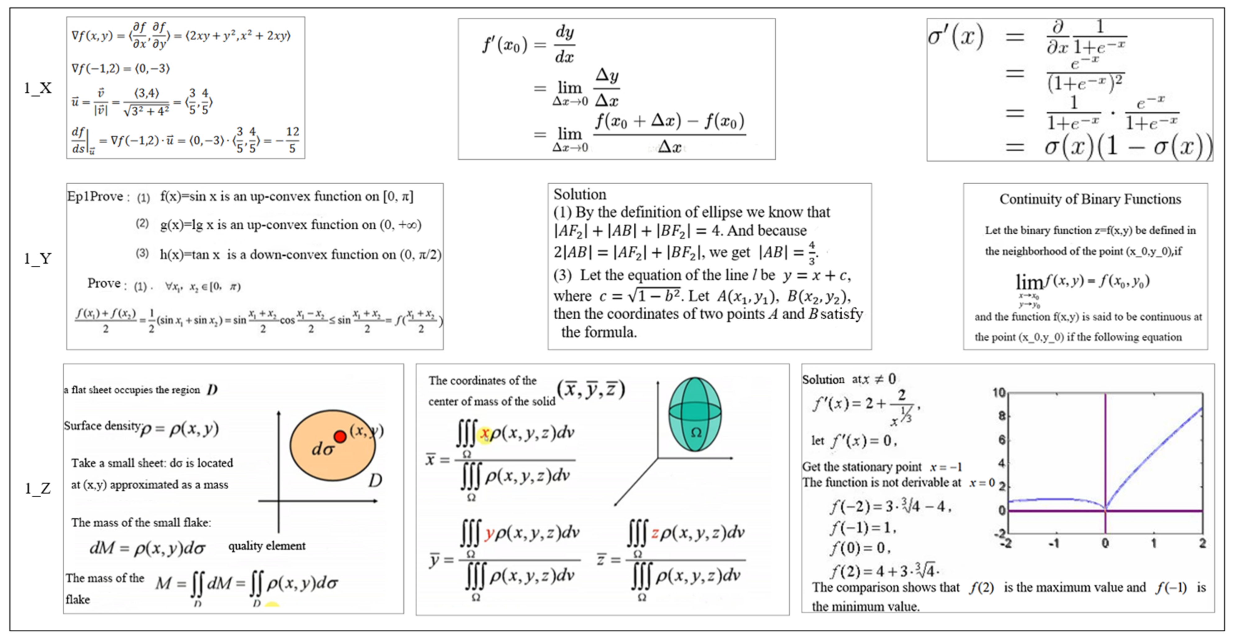
As can be found from the example dataset in Section 3.1.1, mathematical formula images can also be subdivided into several subcategories. This section divides the mathematical formula images into three subcategories, as shown in Figure 10.

Take 100 images of each subcategory and add another 300 images. Image classification is performed using a trained AttNeSt network model. The aim is to verify whether the model has good classification performance for images with formulas interspersed between other elements. The results are shown in

Table 9. Results of the screening.

Type	Correct (1)	Mistake (0)	Correct (0)	Mistake (1)
1_X	100	0	290	10
1_Y	90	10
1_Z	88	12

. Correct and Mistake in Table 9 have the same meaning as in Section 3.4.2.

The results in Table 9 show that all images in subcategory 1_X are correctly classified, two images in subcategory 1_Y are misclassified to category 0, and 12 images in subcategory 1_Z are misclassified to category 0. In addition, 10 of the 300 other images were misclassified to category 1. Overall, the model has superior performance for classifying images with only mathematical formulas, and good performance for images with formulas interspersed between text or coordinate diagrams.

4. Conclusions

To screen images containing mathematical formulas in web pages or scientific documents, we designed a network model, AttNeSt, that can screen images containing mathematical formulas from among many kinds of images. First, the feature correlation enhancement (FCE) module was designed with the aim of improving the contribution of mathematical formula features in the self-attention feature maps. Then, the strip multi-scale pooling (SMP) module was designed to cause the input images to retain their original sizes and to focus on horizontal formula features. Finally, regularization is incorporated into the binary cross-entropy loss function to balance the dataset. The experimental results show that the ACC of AttNeSt is 7.18% better than ResNeSt. The superior performance of AttNeSt compared with other methods. Good results were obtained using the trained AttNeSt network model to screen the blended images, as shown in the results of Section 3.4.2 and Section 3.4.4 For images where mathematical formulas are interspersed with text or illustrations, etc., the model is able to screen most of these images correctly.

Although the model in this paper can accurately screen images containing mathematical formulas in most cases, there are errors. For example, mathematical formulas are also present in Figure 8g, but they were classified into category 0. The reason for the classification error is that the mathematical formula part of the figure is too small in proportion to the rest of the image. In addition, embedded formulas, edge formulas not easily recognized, and formulas interspersed with text where features are difficult to distinguish may also cause classification errors. The follow-up work will include continued theorizing about new approaches to improve the experiment and achieve better screening results.

The trained AttNeSt network model can screen out images containing mathematical formulas from a large number of images, which helps to facilitate the creation of a database of mathematical formula images. In subsequent work, images within a large number of relevant documents or web pages will be crawled, and images containing mathematical formulas will be screened using the AttNeSt model. This will increase the number of mathematical formula images, which will be helpful for the training of mathematical formula retrieval, formula extraction, and identification, and thus making it more beneficial for readers to be able to retrieve the mathematical formulas they want.

References

- Su, F.; Lv, Q.; Luo, R.Z. A review of image classification research based on deep learning. Telecommun. Sci. 2019, 35, 58–74. [Google Scholar]
- Kim, P. Convolutional neural network. In MATLAB Deep Learning; Apress: Berkeley, CA, USA, 2017; pp. 121–147. [Google Scholar]
- Yang, J.F.; Qiao, P.R.; Li, Y.M.; Wang, N. A review of research on machine learning classification problems and algorithms. Stat. Decis. Mak. 2019, 35, 36–40. [Google Scholar]
- Gao, Q.; Lim, S.; Jia, X. Hyperspectral image classification using convolutional neural networks and multiple feature learning. Remote Sens. 2018, 10, 299. [Google Scholar] [CrossRef] [Green Version]
- Yu, J.; Zhang, C.; Wang, S. Multichannel one-dimensional convolutional neural network-based feature learning for fault diagnosis of industrial processes. Neural Comput. Appl. 2021, 33, 3085–3104. [Google Scholar] [CrossRef]
- LeCun, Y. LeNet-5, Convolutional Neural Networks. Available online: http://yann.lecun.com/exdb/lenet (accessed on 10 December 2020).
- Krizhevsky, A.; Sutskever, I.; Hinton, G.E. ImageNet classification with deep convolutional neural networks. Commun. ACM 2017, 60, 84–90. [Google Scholar] [CrossRef]
- Zhou, J.Y.; Zhao, Y.M. Application of convolution neural network in image classification and object detection. Comput. Eng. Appl. 2017, 53, 34–41. [Google Scholar]
- Xie, S.; Girshick, R.; Dollár, P.; Tu, Z.; He, K. Aggregated residual transformations for deep neural networks. In Proceedings of the IEEE conference on computer vision and pattern recognition, Honolulu, HI, USA, 21–26 July 2017; pp. 1492–1500. [Google Scholar]
- Wu, Z.; Shen, C.; Van Den Hengel, A. Wider or deeper: Revisiting the resnet model for visual recognition. Pattern Recognit. 2019, 90, 119–133. [Google Scholar] [CrossRef] [Green Version]
- Szegedy, C.; Vanhoucke, V.; Ioffe, S.; Shlens, J.; Wojna, Z. Rethinking the inception architecture for computer vision. In Proceedings of the IEEE conference on computer vision and pattern recognition, Las Vegas, NV, USA, June 26–July 1 2016; pp. 2818–2826. [Google Scholar]
- Szegedy, C.; Ioffe, S.; Vanhoucke, V.; Alemi, A.A. Inception-v4, inception-resnet and the impact of residual connections on learning. In Proceedings of the Thirty-First AAAI Conference on Artificial Intelligence, San Francisco, CA, USA, 4–9 February 2017. [Google Scholar]
- Zhang, H.; Wu, C.; Zhang, Z.; Zhu, Y.; Lin, H.; Zhang, Z.; Smola, A. Resnest: Split-attention networks. arXiv 2020, arXiv:2004.08955. [Google Scholar]
- Ma, W.; Yang, Q.; Wu, Y.; Zhao, W.; Zhang, X. Double-branch multi-attention mechanism network for hyperspectral image classification. Remote Sens. 2019, 11, 1307. [Google Scholar] [CrossRef] [Green Version]
- Liu, S.; Lin, T.; He, D.; Li, F.; Wang, M.; Li, X.; Ding, E. Adaattn: Revisit attention mechanism in arbitrary neural style transfer. In Proceedings of the IEEE/CVF International Conference on Computer Vision, Montreal, QC, Canada, 10–17 October 2021; pp. 6649–6658. [Google Scholar]
- Niu, Z.; Zhong, G.; Yu, H. A review on the attention mechanism of deep learning. Neurocomputing 2021, 452, 48–62. [Google Scholar] [CrossRef]
- Hu, J.; Shen, L.; Sun, G. Squeeze-and-excitation networks. In Proceedings of the IEEE Conference on Computer Vision and Pattern Recognition, Salt Lake City, UT, USA, 18–22 June 2018; pp. 7132–7141. [Google Scholar]
- Wang, C.Y.; Liao, H.Y.M.; Wu, Y.H.; Chen, P.Y.; Hsieh, J.W.; Yeh, I.H. Selective kernel networks. In Proceedings of the IEEE/CVF Conference on Computer Vision and Pattern Recognition, Long Beach, CA, USA, 15–20 June 2019; pp. 510–519. [Google Scholar]
- Gao, W.; Zhang, L.; Teng, Q.; He, J.; Wu, H. DanHAR: Dual attention network for multimodal human activity recognition using wearable sensors. Appl. Soft Comput. 2021, 111, 107728. [Google Scholar]
- He, K.; Zhang, X.; Ren, S.; Sun, J. Spatial pyramid pooling in deep convolutional networks for visual recognition. IEEE Trans. Pattern Anal. Mach. Intell. 2015, 37, 1904–1916. [Google Scholar] [CrossRef] [Green Version]
- Hou, Q.; Zhang, L.; Cheng, M.M.; Feng, J. Strip pooling: Rethinking spatial pooling for scene parsing. In Proceedings of the IEEE/CVF Conference on Computer Vision and Pattern Recognition, Seattle, WA, USA, 13–19 June 2020; pp. 4003–4012. [Google Scholar]
- Ruby, U.; Yendapalli, V. Binary cross entropy with deep learning technique for image classification. Int. J. Adv. Trends Comput. Sci. Eng. 2020, 9, 10. [Google Scholar]
- Li, B.; Lima, D. Facial expression recognition via ResNet-50. Int. J. Cogn. Comput. Eng. 2021, 2, 57–64. [Google Scholar] [CrossRef]
- Zhao, H.; Jia, J.; Koltun, V. Exploring self-attention for image recognition. In Proceedings of the IEEE/CVF Conference on Computer Vision and Pattern Recognition, Seattle, WA, USA, 13–19 June 2020; pp. 10076–10085. [Google Scholar]
- Yuan, M.Y.; Zhou, C.S.; Huang, H.B.; Hu, C.Y.; Li, Y. A review of pooling methods for convolutional neural networks. Softw. Eng. Appl. 2020, 9, 360. [Google Scholar]
- Chen, L.; Liu, C.; Chang, F.; Li, S.; Nie, Z. Adaptive multi-level feature fusion and attention-based network for arbitrary-oriented object detection in remote sensing imagery. Neurocomputing 2021, 451, 67–80. [Google Scholar] [CrossRef]
- Ding, X.; Larson, E.C. Incorporating uncertainties in student response modeling by loss function regularization. Neurocomputing 2020, 409, 74–82. [Google Scholar] [CrossRef]
- Zhou, D.; Fang, J.; Song, X.; Guan, C.; Yin, J.; Dai, Y.; Yang, R. Iou loss for 2d/3d object detection. In Proceedings of the 2019 International Conference on 3D Vision(3DV), Québec, QC, Canada, 16–19 September 2019; pp. 85–94. [Google Scholar]
- Utsugi, M. 3-D inversion of magnetic data based on the L1–L2 norm regularization. Earth Planets Space 2019, 71, 73. [Google Scholar] [CrossRef] [Green Version]
- Li, F.; Zurada, J.M.; Wu, W. Smooth group L1/2 regularization for input layer of feedforward neural networks. Neurocomputing 2018, 314, 109–119. [Google Scholar] [CrossRef]
- Deng, Y.; Kanervisto, A.; Ling, J.; Rush, A.M. Image-to-markup generation with coarse-to-fine attention. In Proceedings of the 34th International Conference on Machine Learning, Ningbo, China, 9–12 July 2017; pp. 980–989. [Google Scholar]
- Zhang, Y.; Xing, K.; Bai, R.; Sun, D.; Meng, Z. An enhanced convolutional neural network for bearing fault diagnosis based on time–frequency image. Measurement 2020, 157, 107667. [Google Scholar] [CrossRef]
- Ge, Y.Z.; Liu, H.; Wang, Y.; Xu, B.L.; Zhou, Q.; Shen, F.R. A review of deep learning image recognition under the dilemma of small samples. J. Softw. 2022, 33, 193–210. [Google Scholar]
- Wang, X.R.; Zhang, H. Small sample classification network based on attention mechanism and graph convolution. Comput. Eng. Appl. 2021, 19, 164–170. [Google Scholar]
- Shorten, C.; Khoshgoftaar, T.M. A survey on image data augmentation for deep learning. J. Big Data 2019, 6, 60. [Google Scholar] [CrossRef]
- Mikołajczyk, A.; Grochowski, M. Data augmentation for improving deep learning in image classification problem. In Proceedings of the 2018 International Interdisciplinary PhD Iorkshop (IIPhDW), Świnoujście, Poland, 9–12 May 2018; pp. 117–122. [Google Scholar]
- Sekaran, S.A.R.; Lee, C.P.; Lim, K.M. Facial emotion recognition using transfer learning of AlexNet. In Proceedings of the 2021 9th International Conference on Information and Communication Technology (ICoICT), Hotel NEO Malioboro, Yogyakarta, Indonesia, 6–8 March 2018; pp. 170–174. [Google Scholar]
- Hussain, M.; Bird, J.J.; Faria, D.R. A study on cnn transfer learning for image classification. In UK Workshop on Computational Intelligence; Springer: Cham, Switzerland, 2018; pp. 191–202. [Google Scholar]
- Lu, T.; Han, B.; Chen, L.; Yu, F.; Xue, C. A generic intelligent tomato classification system for practical applications using DenseNet-201 with transfer learning. Sci. Rep. 2021, 11, 15824. [Google Scholar] [CrossRef]
- Sun, P.; Jin, X.; Su, W.; He, Y.; Xue, H.; Lu, Q. A Visual Inductive Priors Framework for Data-Efficient Image Classification. In European Conference on Computer Vision; Springer: Cham, Switzerland, 2020; pp. 511–520. [Google Scholar]
Figure 1.
AttNeSt network structure diagram.
Figure 2.
Structure of FCE module.
Figure 3.
Structure of SMP module.
Figure 4.
Examples of images. Figure (a) contains only mathematical formulas. Figure (b) contains coordinate axes, formulas, and text. Figure (c) contains mathematical formulas and text. Figure (d) contains formulas, text and other images.
Figure 5.
Variation of ACC in the training set and validation set of AttNeSt.
Figure 6.
Loss variation curve. BC denotes the binary cross-entropy loss function, and IBC denotes the improved loss function.
Figure 7.
Loss variation by algorithm.
Figure 8.
Image example. In the figure (a,b) images have formulas and a small amount of text, (c,d) images contain only mathematical formulas, (e–h) images are cases in which formulas are interspersed with text, the (f) image contains only text, and (i–l) images do not contain mathematical formulas.
Figure 9.
Example of im2latex-100k dataset images.
Figure 10.
Examples of subcategories of images. The 1_X category represents an image that contains only mathematical formulas, the 1_Y category represents an image that contains both text and mathematical formulas, and the 1_Z category represents an image that contains both text, coordinate maps and formulas.