Solpen: An Accurate 6-DOF Positioning Tool for Vision-Guided Robotics

Abstract

A robot trajectory teaching system with a vision-based positioning pen, which we called Solpen, is developed to generate pose paths of six degrees of freedom (6-DoF) for vision-guided robotics applications such as welding, cutting, painting, or polishing, which can achieve a millimeter dynamic accuracy within a meter working distance from the camera. The system is simple and requires only a 2D camera and the printed ArUco markers which are hand-glued on 31 surfaces of the designed 3D-printed Solpen. Image processing techniques are implemented to remove noise and sharpen the edge of the ArUco images and also enhance the contrast of the ArUco edge intensity generated by the pyramid reconstruction. In addition, the least squares method is implemented to optimize parameters for the center pose of the truncated Icosahedron center, and the vector of the Solpen-tip. From dynamic experiments conducted with ChArUco board to verify exclusively the pen performance, the developed system is robust within its working range, and achieves a minimum axis-accuracy at approximately 0.8 mm.

1. Introduction

In the demanding workflow of the robotics and manufacturing industry, the need for a more natural human-robot interaction is rather high when increasingly-popular complex tasking scenarios, including human-robot, and multi-robot collaboration, are considered. A natural and efficient robot teaching method would alleviate the need for current time-consuming robot programming effort. In addition, robot teleoperation in disasters, rescue missions or toxic working environments are in demand. These applications are not merely bound to conceptualization. In 2016, a Yaskawa Motoman SIA5D could be accurately teleoperated by Kruusamae and his colleagues to thread needles of different sizes [1]. Tsarouchi et al. [2] proposed a visual-based robot programming system using the motion capture sensor Leap Motion Controller. Gesture vocabularies were designed to be translated to robot primitive motion commands to program single and bi-manual robots.

Manou et al. demonstrated robot teaching by demonstration for robot seam welding, deburring or cutting applications where the project deployed industry-grade photogrammetry software and hardware to build the system [3]. A 6 degree-of-freedom flock-of-bird magnetic sensor is used to allocate a hand-held teaching device and coded targets are placed on the workpiece for its calibration. The research attempted to validate the accuracy by comparing the operator teaching path and robot executed path. However, this validation is solely conducted once with 5 trajectory points. Their implementation was mainly restricted by the accuracy of the magnetic sensor, which is up to 1.8 mm in position.

2. Related Work

The research in [4] proposed a robot teaching method very closely related to our work with regards to the type of interaction, which also relies on a pen whose pose is to be replicated by the taught robot. However, our method differentiates from the customization and the design of the overall vision-based pen pose detection whereas their method utilizes a commercial motion capture system. More specifically, the proposed teaching system includes a teach pen, motion capture markers on the pen, a motion capture camera, and a pose estimation algorithm given in the hardware. They employ a Human-Computer Interaction (HCI) evaluation scheme based on Fitts’ law to compare to more traditional teaching systems. In the experiment, their system concluded to achieve an average error of 1.3 mm.

With natural interaction frameworks and low-cost 3D sensors becoming popular, one research paper [2] followed the trend to seek more natural human robot interaction by building upon human gesture vocabulary using off-the-shelf and low cost 3D sensors e.g., Microsoft Kinect, Leap Motion while the solution was built on the availability of low-level gesture detection framework, e.g., OpenNI. The system was also integrated into theROS middleware framework to facilitate future extensibility. However, the method is more suitable for less accuracy demanding applications due to the noise susceptible vision-based detection. The vocabulary, either from the body or hand gestures, is built from 6 primitive motions in the human frame including $\pm X,\pm Y,\pm Z$. The system was evaluated in a case study of the automobile industry to assemble a dashboard to a vehicle. The test case includes four different operations and the recognition success rate reached more than 93%.

In [5,6], a robot teaching by demonstration framework is proposed to accomplish an assembly sequence of several pick-and-place tasks. The scheme is made possible by deploying multiple recent advances in the field including scene reconstruction, 3D object recognition, and augmented reality (AR). More concretely, scene reconstruction allows scene understanding, and 3D object recognition allocates workpieces in the working space. An AR algorithm on the user mobile device enables virtual object interaction which in turn defines the task sequence. The authors discussed in detail the proposed markerless pipeline to define a trajectory using hand gestures in the follow-up work [6].

Arpen [7] represents a series of studies with a similar approach to a HCI. The pen is designed with a cube shape, and the study is limited to six markers, with each adjacent pair having a 90-degree angle. This results in a decrease in performance when only one marker is within the view. Even when two markers are available, the large angle between adjacent markers leads to a strong differentiation in light shading of the sides and, therefore, affects the detection result. Nevertheless, their design verification aims at a user’s ease of use and maneuvering efficiency.

The work of [8] is an astounding project that exhibits a convincing performance of a 3D tracking pen with ArUco markers attached on a dodecahedron at its end. The pen aims to accomplish normal writing with an achievable 250 fps captured by a 1.3 MP camera. The system accuracy was extensively tested with an optical Coordinate Measurement Machine (CMM) system and reached sub-millimeter precision. The validation also includes trajectory tracking under different settings overlaid on the ground-truth trajectories. This result convinced us to deploy to our robot trajectory training system. However, their design limits the number of markers seen by the camera at each captured frame, which hinders the system accuracy in critical applications. We explore an extension to this design, allowing more markers to be seen. In addition, we utilize a distinct approach to evaluate the overall accuracy without the need of an optical CMM system. Even though such a system can offer a high accuracy guaranteed ground-truth, it unavoidably adds a significant cost to the development. We chose a statistics-based method for accuracy verification with validated sub-millimeter results. The results are also empirically validated. In addition, we provide a demo video as a Supplementary Material.

3. System Description

3.1. Bundle Adjustment

From [9], the authors aimed to bridge the gap between the concurrent research in computer vision’s 3D reconstruction and related topics versus previous ones in photogrammetry. The author spotted a repetitive reinvention of the know-how that had formed the foundation of photogrammetry and theory of estimation long ago. Along with other extensive works in photogrammetry such as [10], the authors revealed a lack of emphasis on the evaluation and validation of the estimation process existing in common practice in computer vision engineering.

In light of [9,10], it is beneficial to adopt know-hows from photogrammetry to form the measures that assist practitioners to inspect and evaluate the results. Such a foundation has been well-established in the quality control stage of a photogrammetry workflow. These procedures, to some extent, still mostly involve expert ad-voc heuristics and experiences to design specific workflow for a project. We also would like to point out such challenges, specifically regarding the working project [9,10], which, however, undertook excellent work in outlining the main topics and fundamental conceptions.

In [9], the term internal reliability is used to address the system’s ability to detect and eliminate outliers which, in turn, is realized by robust estimation or classic outlier detection. External reliability, on the other hand, is the ability of the system to withstand the undetected outliers and still retain the estimation performance. Ref. [10] discussed similar nomenclatures, but perhaps in a more concrete way. Diagnostics is the process to find and identify deviations from the model assumptions. Robustness, in contrast, is the safeguarding against deviations from the assumptions.

The author continues to classify diagnostics to internal and external diagnostics. Internal diagnostics, besides the aim to look for outliers, aims to find general model deviations, and therefore includes both the mathematics model and noise model of the system, and the tests to identify the causes. However, as pointed out, the math model deficiencies and observation errors cannot be differentiated by internal diagnostics. External diagnostics assumes the availability of ground truth data; therefore, it allows a distinction between model deviations and observation errors which makes it possible to achieve stronger conclusions on the estimated uncertainty, efficiency, and robustness of the estimation. A foremost test that can be readily performed at an early development stage is the correctness check. This can be conducted using a toy problem on simulated data to verify the implementation with respect to theoretical assumptions.

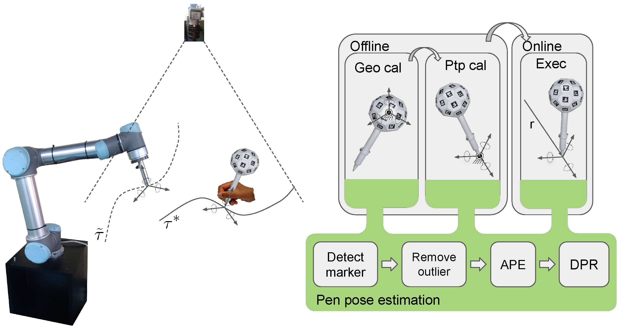
3.2. Workflow Overview

The algorithm consists of two major phases for the 6-DoF reconstruction of the Icosapen tip: (1) approximate pose estimation (APE) phase and (2) dense pose refinement (DPR) phase. Firstly, the Basler camera is fixed on a rigid frame and calibrated by the checkerboard $7\times 9$ (the squares side is 20 mm) to obtain the camera matrix and distortion coefficients. We then conduct a video recording and apply both APE and DPR to obtain optimized initial transformations from 31 detected ArUco faces to the center of the designed truncated Icosahedron. From these optimized transformations, we implement the pen tip calibration by rotating the pen tip around a fixed point as in Figure 1 to gather training points that should be located on a spherical surface. The center of the sphere is trained and optimized to identify its position in the camera coordinate from the spherical dataset. Finally, the pen tip vector from the center of the Icosahedron is used to identify the pose of the pen tip in the camera coordinate. The overall process is shown in Figure 1.

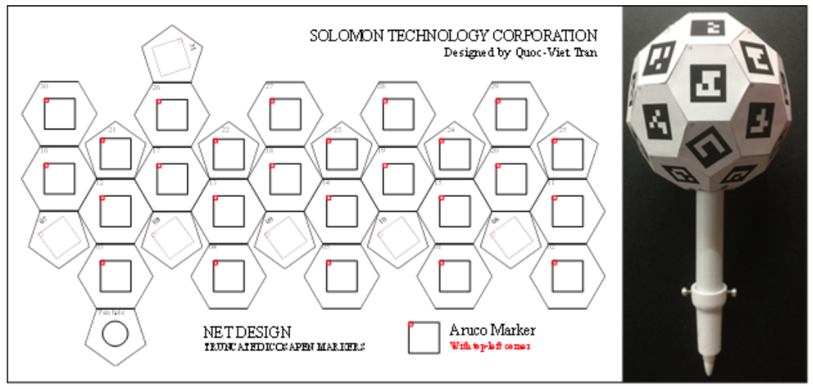
3.3. Icosahedron Design

The Truncated IcosaHedron (Wikipedia contributors, “Truncated icosahedron”, Wikipedia, The Free Encyclopedia, https://en.wikipedia.org/w/index.php?title=Truncated_icosahedron&oldid=1017030761 (accessed on 4 May 2021)) geometry is constructed from Icosahedron (Wikipedia contributors, “Icosahedron”, Wikipedia, The Free Encyclopedia, https://en.wikipedia.org/w/index.php?title=Icosahedron&oldid=1021031901 (accessed on 4 May 2021)) with the 12 vertices truncated such that one-third of each edge is trimmed at each of both ends. It generates a polyhedron consisting of 32 surfaces (12 pentagonal and 20 hexagonal faces), 60 vertices, and 90 edges. The coordinate of the truncated icosahedron is defined at the center and vertices are a combination of 3D points belonging to the orthogonal rectangles $(0,\pm 1,\pm 3\phi )$, $(\pm 1,\pm 3\phi ,0)$, $(\pm 3\phi ,0,\pm 1)$ and the orthogonal cuboids $(\pm 2,\pm (1+2\phi ),\pm \phi )$, $(\pm (1+2\phi ),\pm \phi ,\pm 2)$, $(\pm \phi ,\pm 2,\pm (1+2\phi \left)\right)$ along with the orthogonal cuboids $(\pm 1,\pm (2+\phi ),\pm 2\phi )$, $(\pm (2+\phi ),\pm 2\phi ,\pm 1)$, $(\pm 2\phi ,\pm 1,\pm (2+\phi \left)\right)$, where $\phi =(1+\sqrt{5})/2$ is the golden mean. Using $\phi 2=\phi +1$ one verifies that all vertices are on a sphere, centered at the origin, with the radius squared equal to $9\phi +10$. The edges have a length of 2 mm. We scale edge length into 25 mm for the proposed truncated Icosapen design as shown in Figure 2.

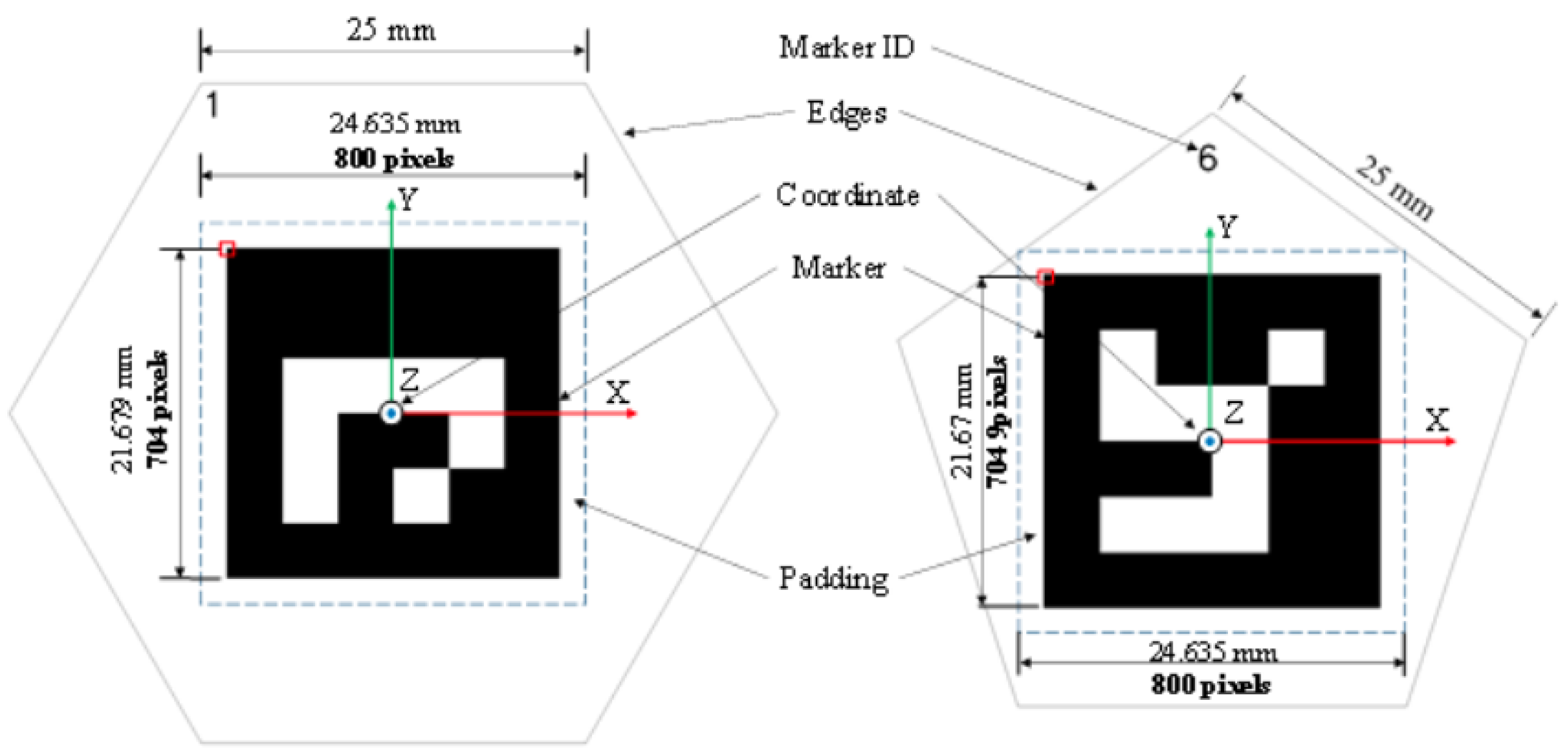
3.4. Define Aruco Marker Poses in Penta and Hexa-Polygon

ArUco markers were originally developed by S.Garrido-Jurado [11]. These markers are highly reliable under occlusion when they are used in a set, e.g., ArUco, ChArUco board [12]. A single ArUco marker is a binary square composed of a wide black border and an internal binary matrix to identify its identifier (ID). Currently, there are more than 25 dictionaries of markers that are widely applied in various applications with different binary block sizes ($4\times 4$, $5\times 5$, $6\times 6$, $7\times 7$). The binary grid size of the marker type is proportional to the possibility of the maximum number of generated markers. From truncated Icosahedron design, a pentagonal surface is utilized to mount the pen, as shown in Figure 3, only 31 surfaces (11 pentagonal and 20 hexagonal faces) are available to glue markers. In this study, the ArUco dictionary DICT_4X4_50 (grid $4\times 4$, the maximum generated marker is 50) is used to generate markers with the IDs from 1 to 31. Since the edge length of the truncated Icosahedron geometry is 25 mm, the real marker length is approximately 22 mm which is quite small to detect at a far distance. Therefore, the $4\times 4$ binary block will increase the detail of the ArUco image at far distances compared to the others. The center of each marker is aligned with the center of the pentagonal or hexagonal surfaces, as shown in Figure 3. The full design of the Solpen Net is illustrated as Figure 4

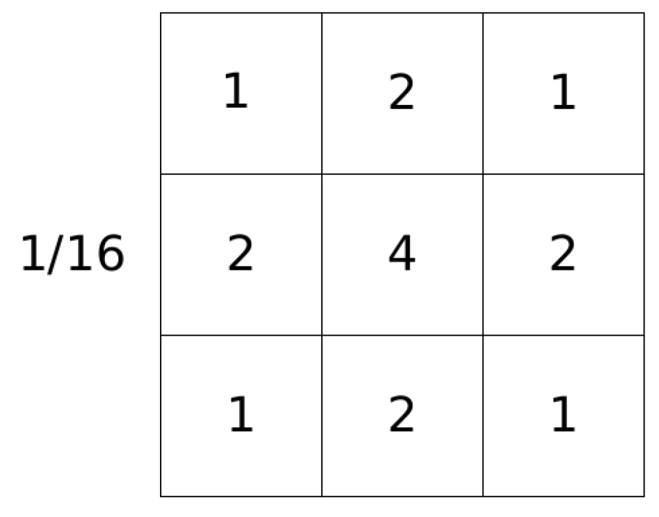
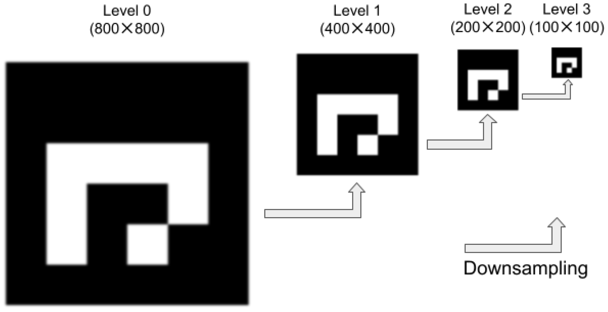
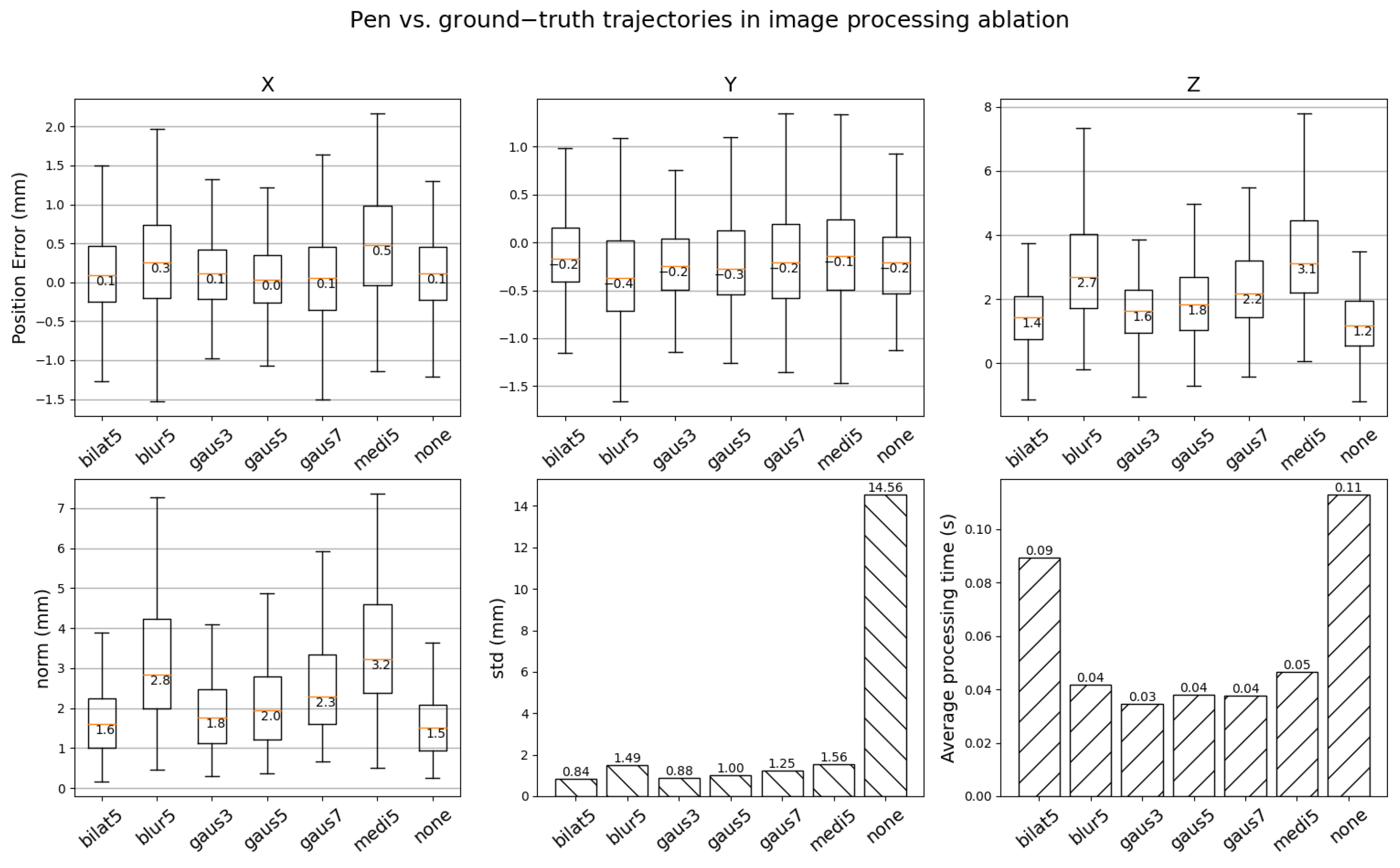
3.5. Image Enhancement/Processing Pipeline

Preprocessing Images

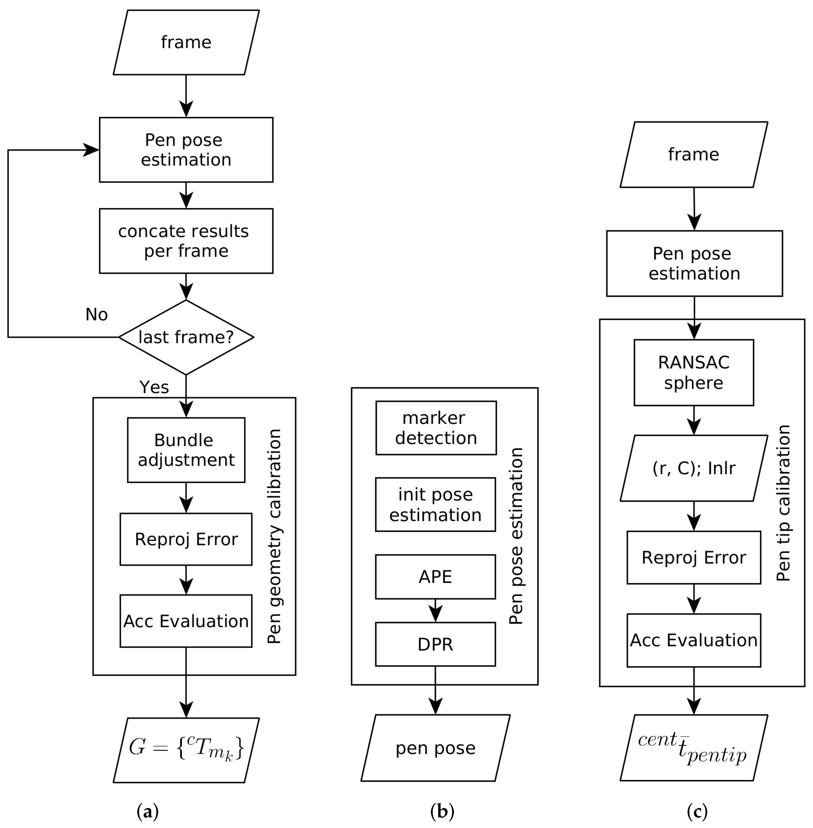
Since VR Icosapen is usually used to draw with a diverse range of moving speed within a meter square working space of the Universal Robot (UR5), the image can be blurred with fast motions or at a close distance that is out of the Depth-of-Field. This results in a poor performance for localizing the poses of the ArUco markers. Moreover, image noise is significantly increased around the edge of the ArUco markers at a far distance, resulting in incorrect corner detection. Therefore, removing noise and retaining sharp image edges play a pivotal role in improving the accuracy of the pen tip pose estimation.

We first eliminate image blur by using an industry standard camera (Basler) that can control the capturing exposure time and possess significantly less noise due to the high quality image sensor to ensure the best image quality. A non-linear bilateral filter is then implemented to further reduce noise and preserve the sharpness of the ArUco markers’ edges. A typical spatial filtering applied on image I to obtain image $I_F$ is given by Equation (1)

$$I_F\left(x\right)=\frac{{\sum }_{x_i\in \mathsf{\Omega }}w\left(x_i\right)I(x+x_i)}{{\sum }_{x_i\in \mathsf{\Omega }}w\left(x_i\right)}$$

(1)

This is basically a weighted sum operation performed at each pixel location x with the weight value w indexed from the neighboring pixel $\mathsf{\Omega }$. There are several choices for the weight mask/kernel. The Gaussian kernel (shown in Figure 5) is a popular kernel.

A bilateral filter not only attenuates in spatial domain with weight $w_s$ but also in the range/intensity domain by an additional term $w_r$, and it is defined in Equation (2) below:

$$I_{BF}\left(p\right)=\frac{{\sum }_{q\in \mathsf{\Omega }}{I}_q{w}_r\left(\parallel I_q-I_p\parallel \right)w_s\left(\parallel q-p\parallel \right)}{{\sum }_{q\in \mathsf{\Omega }}{w}_r\left(\parallel I_q-I_p\parallel \right)w_s\left(\parallel q-p\parallel \right)}$$

(2)

where $I_{BF}$ is a filtered image by the bilateral filter; I is the source image; p are coordinates of the current processing pixel to be filtered; $\mathsf{\Omega }$ is the window kernel centering at p pixel, q are the neighbouring pixels; $w_r$ and $w_s$ are the weight kernels for range and spatial domains which are commonly chosen to be Gaussian kernels.

Since the kernels are Gaussian, the combined weight can be readily derived by exponent multiplication (Equation (3))

$$w_{BF}(p,q)=w_r{w}_s=exp\left(-\frac{\parallel I_q-I_p{\parallel }^2}{2{\sigma }_r^2}-\frac{{\parallel q-p\parallel }^2}{2{\sigma }_s^2}\right)$$

(3)

where ${\sigma }_r$ and ${\sigma }_s$ are the variance which we chose to be a similar value 75 with a kernel size 5 in the implementation; $I_q$ and $I_p$ are the intensity of pixels p and q, respectively. Substitute Equation (3) into Equation (1), and the formulation for a bilateral filter applied on an image is as follows:

$$I_{BF}\left(p\right)=\frac{{\sum }_{q\in \mathsf{\Omega }}{I}_q{w}_{BF}(p,q)}{{\sum }_{q\in \mathsf{\Omega }}{w}_{BF}(p,q)}$$

(4)

With the non-linear bilateral filter, the gradient at image edges is reserved better, which could help to avoid false ArUco edges in an image. The false edges also cause the presented APE approach to perform poorly due to the false corner detection of ArUco markers. To tackle this issue, we generate a gradient at the edges of the ArUco markers by extending zero paddings to the original ArUco marker. The original marker size is designed with resolution $704\times 704$ and extended with padding to have the full resolution $800\times 800$ as shown in Figure 3. We then first build Gaussian Pyramid images of four levels ($800\times 800$, $400\times 400$, $200\times 200$, $100\times 100$, $50\times 50$) from all 31 generated markers with a padding extension and then reconstruct from the Gaussian Pyramid images to generate a blending effect at the edges of the ArUco markers. The detailed pyramid image reconstruction is visualized in Figure 6.

The APE algorithm first estimates the approximate positions of four corners from each detected ArUco marker. These corners are then used to interpolate the position of four padding corners in order to enhance the contrast by normalizing the inside pixels into the range (0–255). The Dense Pose Refinement (DPR) is then implemented so that the intensity of gradient pixels at the detected ArUco edges are then aligned with the intensity pixels at the edges of the generated pyramid reconstruction ArUco image to refine the accurate four corners of each detected ArUco marker.

4. Pen Calibration

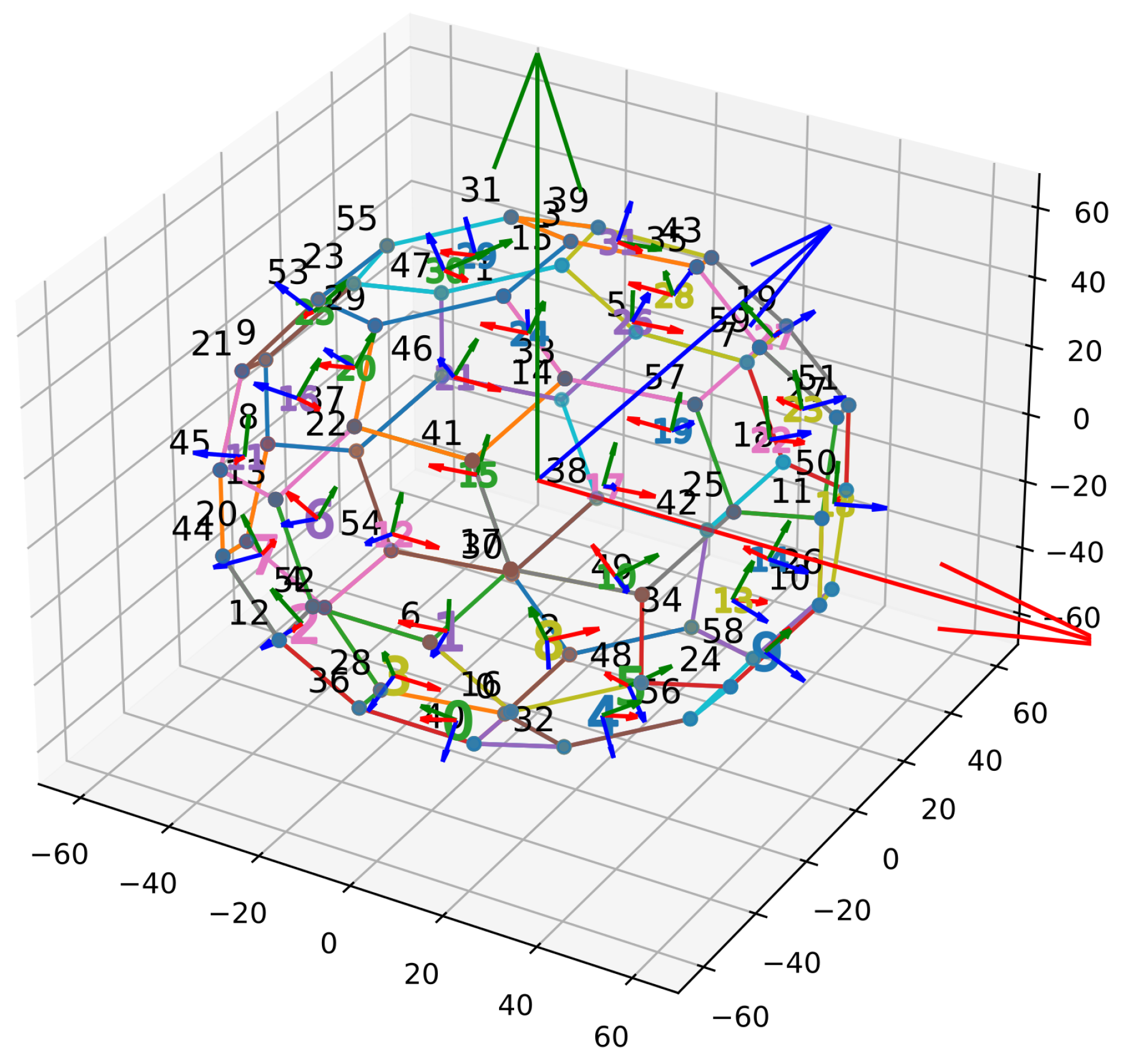
4.1. Pen Geometry Calibration with Bundle Adjustment

As the AR printing markers are attached to the pen surfaces, such an attachment process might be carried out by manual work and is vulnerable to operational errors. In addition, the pen shape formed by low cost manufacturing is also subject to errors. This overall geometry error accounts for the 3D relative transformation error between the attached markers. The error is estimated by using a reformulated Bundle Adjustment (BA) algorithm.

As we have already known, BA packed the estimation of structures, camera view poses and its intrinsics together in the unknown. In our case, we finished camera calibration in advance of BA procedure be cause the intrinsics calibration is a well-formed process of its own and, therefore, it can be decoupled to avoid unnecessary complication.

In our scenario, the pen calibration has multiple modalities of prior knowledge to take advantage of. The structures of the fiducial markers, namely its sizes and expected arrangement are known at the early design stage. The camera view poses in the sequence of image captures can also be estimated by pose estimation methods such as perspective-n-points and can be used as initialization. These factors make it possible for the estimation to achieve detailed structures with 3D poses of the calibrated markers.

Briefly, the BA algorithm estimates the unknown by relying on measurable equations which are generally quantified by reprojection errors. More precisely, these reprojection error equations are presented in Equation (5):

$$e^{ij}=p^{ij}-\mathsf{\Pi }{(}^c{T}_p{.}^p{T}_{m_0}.M^0)$$

(5)

where $e^{ij}$ are the reprojection errors, $i=1,\dots ,F$ is frame i-th index and F is total number of frames; $j=1,\dots ,P$ is image point j-th index and P is total number of image points; ${}^c{T}_p$ is the coordinate transformation from pen c.s. to camera c.s.; ${}^p{T}_{m_0}$ is the coordinate transformation from marker-0 c.s. to pen c.s.; $M^0$ is a model/marker point in marker-0 c.s. $\mathsf{\Pi }$ is the pin-hole camera projection. Pen c.s. $\left\{p\right\}$ is illustrated in Figure 1.

Equation (5) is assembled to form an optimization problem in which the unknown x is the concatenated of the vectorized version of ${}^c{T}_{m_k}$ where $k=1,\dots ,K$ and K is the number of markers; or in set notation, the unknown is a set of homogeneous transformation $G={\{}^c{T}_{m_k}\}$. This formulates Equation (6) as followed:

$$x^{\ast }=\underset{x}{argmin}\sum _{ij}{e}_{ij}^T{e}_{ij}$$

(6)

Equation (6) is therefore formed as a nonlinear least square problem and is solved by an available optimization solver. The implementation of geometry calibration is facilitated by the pipeline of Figure 7a.

4.1.1. Approximate Pose Estimation (APE)

We rotate all possible views of the Solpen and simultaneously record 5000 frames for geometry calibration. Similar to Bundle Adjustment, we first compute center poses of the Icosahedron by multiplying the designed surface-to-center transformation matrices with the detected poses of the corresponding ArUco marker poses. All center poses are then clustered by the Euclidean distance to remove outlier centers. The inlier center poses are then used to compute the averaging center pose (${}_{cent}^{cam}{T}^k$) of the Icosahedron at frame k. From the new averaging center pose, we optimize the all center-to-face transformation matrices ${}_{cent}^{fac{e}_j}{T}^k$ to minimize 3D reprojection errors of corners on the frame image k by using the Least Square optimization as shown in Equation (7) below

$$min\left(F\left(e\right)\right)=min\sum _k\sum _j\sum _i\left[x_{i,j}^k-\pi \left({}_{cent}^{cam}{T}^k{\ast }_{fac{e}_i}^{cent}{T}^k\ast X_{i,j}^k\right)\right]$$

(7)

where $x_{i,j}^k$ and $X_{i,j}^k$ are 2D and 3D corner i $(i=1,\dots ,4)$ positions of frame k of the detected marker j $(j=1,\dots ,31)$. ${}_{fac{e}_i}^{cent}{T}^k$ is the transformation matrix from the detected marker j to the center of the Icosahedron at frame k, and ${}_{cent}^{cam}{T}^k$ is the transformation matrix of the center pose of the Icosahedron in the 3D camera coordinate. $\pi$ is the pinhole camera projection, including intrinsic and distortion coefficients of the Basler after calibration.

4.1.2. Dense Pose Refinement (DPR)

All inlier corner points obtained from the APE approach are used to localize zero paddings of the detected inlier ArUco markers by scaling with a factor as in the original design shown in Figure 3. Normalization is first applied to scale min-max pixel values inside zero-padding regions into range (0–255). The bilateral filter is then applied to remove noise and to preserve a sharp edge with a gradient effect. These intensity pixels at the gradient transition region are then aligned with the edge gradient pixels built up from the Gaussian pyramid reconstruction so that the total error of intensity pixels is minimized.

From the center poses of the detected ArUco markers, the APE approach is first used to remove outliers and find out the optimized transformation matrices from inlier center poses to optimized center pose of the truncated Icosahedron. The pyramidal Lucas-Kanade algorithm is then implemented to track the local frames containing ArUco markers for boosting computational time. For generating gradient transition band at detected inlier ArUco marker edges from white to black (255, 0 intensity value in gray image, respectively), these local frames with zero padding extension are first normalized into 8-bit image format (pixel value from 0–255) to enhance contrast before filtering with Bilateral filter.

Gaussian image reconstruction technique is also implemented on the designed markers with zero paddings as shown in Figure 3 to generate a gradient transition band from 0 to 255 (black to white) at the edges of the ArUco images. We set upper and lower thresholds of 60 and 160 to extract 2D and 3D pixel positions from the reconstructed images. The corresponding intensities from these pixels are then used to align with the intensity values extracted from the inference frames to refine poses of detected ArUco markers.

4.2. Pen Tip Calibration

To perform pentip calibration, we rotate the Solpen around a fixed hole while maintaining the contact between the pentip and the hole and record a video for the whole motion. Noting that this makes the hole function similar to a spherical joint. The position of the icosahedron center over each recorded frame is expected to lie on a spherical surface, which has its center located at the fixed hole. However, some of these center locations deviate largely from the nominal sphere radius and are considered as outliers. This setting is suitable for a RANSAC spherical fitting algorithm in order to remove outliers with a threshold distance constraint and resolve for the sphere center and its radius. In more precise terms, each frame provides the estimation of the icosahedron pose ${}^{cam}{T}_{cent}$ while the sphere fitting gives a location vector ${}^{cam}{t}_{pentip}$, which is converted to a homogeneous form ${}^{cam}{T}_{pentip}$ with identity rotation, a sphere radius, and inlier flags.

$${}^{cent}{T}_{pentip}^i{=}^{cam}{T}_{cent}^{-1}{.}^{cam}{T}_{pentip}$$

(8)

Noting the relation shown in Equation (8) is repeated for each estimation frame, we leverage it to compute its inlier mean exclusively for the translation (Equation (9)) from the inlier flags

$${}^{cent}{\overline{t}}_{pentip}=E\left(tr{(}^{cent}{T}_{pentip}^i)\right)$$

(9)

where $E(.)$ is the mean operator, $tr(.)$ is the translation of a homogeneous transformation, and i is the frame index. Pen tip calibration is implemented with the pipeline of Figure 7c.

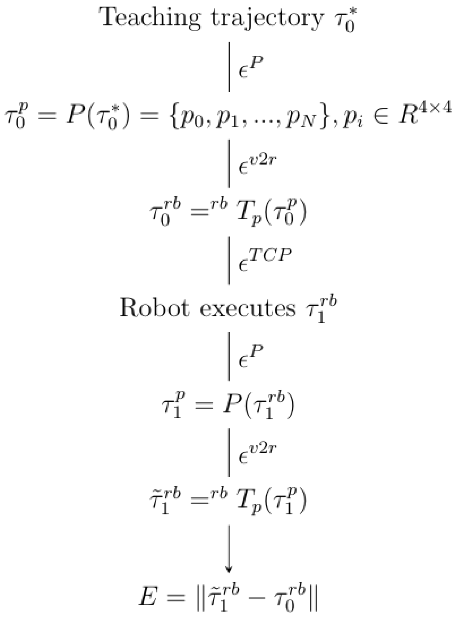
5. Evaluation of a Teaching Operation

With the aim of an efficient robot teaching device, our evaluation goals should involve an actual use case of a robot teaching by an operator and, under such a circumstance, the required accuracy can be attained regardless of the gross error of the overall system. In this particular multistage setup, at stage (1), an operator would use the pen in a free and comfortable way to teach the robot performing a teaching trajectory ${\tau }_0^{\ast }$. At stage (2), The trajectory is captured and estimated by the camera to result in the teaching trajectory in the camera c.s. ${\tau }_0^P$ which consists of a sequence of poses $\{p_0,p_1,\dots ,p_N\}$ where $p_i\in R^{4\times 4}$. This estimation accumulates an error ${ϵ}^P$. At stage (3), the previous trajectory is transformed to robot c.s. to have ${ϵ}_0^{rb}$ by the calibrated vision-to-robot (V2R) which is hindered by the error ${ϵ}^{v2r}$. At stage (4), the robot is commanded to perform the given trajectory with its attached tool (a TCP-calibrated Solpen) which likely has an error ${ϵ}^{TCP}$. At the final stage (5), the executed robot trajectory is estimated by the algorithm to have trajectory in pen c.s. ${\tau }_1^P$. The accuracy evaluation relies on the discrepancy between ${\tau }_0^P$ and ${\tau }_1^P$ at stage (5) under a chosen metric. We picture this evaluation in the diagram in Figure 8.

6. Experiment Results

We divide the evaluation of our system into following stages: geometry calibration, pentip calibration, inference accuracy including static noise and dynamic analysis. To facilitate the experiments, an industrial grade Basler acA1920-155um camera with 8 mm lens is used. This camera configuration provides images with resolution of $1920\times 1200$. It has a CMOS sensor with size 11.3 mm × 7.1 mm with a 1/1.2 in format. With fast motions of the pen under an operator’s normal use, a light setup is necessary which we use a Skier Sunray 200 CUBE dual color temperature LED light with 200 W power, 19,200 lm, the full color temperature range can maintain the real 200 W brightness, high color rendering Color Rendering Index (CRI) 95, color temperature 3000–5700° K. A robot needs to replicate the taught path which we deploy a Universal Robot UR5 robot weighing 18.4 kg, with a 5-kg payload. Its reach is 850 mm and each joint range is from $-360°$ to $+360°$. The overall setup is shown in Figure 9:

6.1. Vision to Robot Calibration

As can be seen in our setup, an industrial-grade CCD camera is placed looking towards the working range. This is called eye-to-hand configuration. In common robot-vision applications, the camera(s) is used as a perception device to assist a robotic actuator to localize the workpiece. Also, the perception is likely achieved in the camera coordinate frame which requires a conversion to the actuator or the execution module frame. This is referred to as vision-to-robot (V2R) calibration. Camera configurations generally include: (1) eye-to-hand: the camera is attached to a fixed pole, looking towards the robot’s end-effector and the workpiece; or (2) eye-in-hand: the camera is attached to the robot’s end-effector, looking towards the workpiece [13]. The literature regarding vision-robot calibration can be quite profound and has been extensively worked over the years since the 80s–90s. Well-known work includes [14,15,16,17] and some recent reviews worth mentioning [18,19]. However, we do not aim to resolve this problem in this work but instead refer readers to the comprehensive research in this field.

To simplify the calibration of this conversion/transformation of coordinates, we leveraged the setup with the Solpen already attached to the robot’s end-effector and is calibrated as the tool-center-point (TCP). This allows the knowledge of both the TCP/pentip locations in robot c.s. and camera c.s. In such a scenario, the solution is the rigid transformation of two sets of 3D points which we deploy a solid algorithm such as in [20]. We took seven point pairs to calibrate the setup. Some of the snapshots on the calibration are shown in Figure 10:

6.2. Accuracy Evaluation

To perform pen calibration, we chose an optimal close-up distance within the focus range to record two videos each one for geometry, and pen tip calibration. With the same purpose to achieve the highest accuracy, the other environment/experiment setups are configured to favour the achievable smallest gross error. Therefore, it also includes the best light setup to minimize random errors in marker detection. The overall parameters affecting this calibration can be listed as: working distance, image brightness (lens aperture, exposure time, lighting), camera resolution. The exposure time is compromised between motion blur and the necessary brightness.

6.2.1. Calibration Accuracy

For geometry calibration, the video is recorded in such a way that each of the markers appears at least in one frame of the video for it to be calibrated. Also, since the operation orients to optimum accuracy, the pen is not necessarily required to move the whole working range of the field-of-view. However, in general, the pen can still move freely and this is contrasted to the case of pentip calibration. In the latter calibration, the pen is moved freely in terms of orientation with a requirement that its pentip is fixed in position. Regardless, the working distance from the pen’s icosahedron to the camera is at an optimally close range. To depict this process, please refer to Figure 11.

To visualize the accuracy of pen calibration, we utilize the standard deviation of the residuals at the optimized solution. This residual plot can assist to validate theoretical assumptions when least square regression is deployed. The assumptions include: homoscedastic, zero-mean, bias, uniformity, or outliers, which Figure 12 has validated. The figure shows these residual plots.

In order to inspect more specifically the distribution of the residuals, we use box plots in Figure 13, which also attempts to visualize the accuracy under different modes of the estimation pipeline, namely, without DPR and without both APE and DPR. The plot visualizes and affirms the effectiveness of the optimization stages of the estimation pipeline. Namely, after pen calibration is done, when estimation is executed upon input streams (i.e., “online” processing) and the full pipeline, i.e., having both APE and DPE merely approximates the one with APE alone. The performance, however, decreases rather clearly when both APE and DPR are not enabled (shown at the right most box of Figure 13).

A timing test on the same recorded camera stream with 500 frames gives a processing time of 185.6 s, 109.1 s, and 75.16 s accordingly for a full algorithm pipeline, one without DPR, and one without both APE, DPR. Without DPR, as shown in Figure 13, the overall algorithm does not significantly affect the estimation performance but the gain in processing time is noticeable i.e., roughly 2 times as long. Such characteristics can be leveraged to improve processing time in necessary scenarios.

6.2.2. Inference Accuracy

Inference accuracy verification can be more comprehensive since this test aims to verify the method performance under varying working conditions within the operational range. Here, we would parameterize the conditions of lighting, working distance, and scenarios including static and dynamic.

Static noise: To perform static noise verification, the pen is placed in approximately similar pose at varied working distances to the camera, i.e., 40 cm, 60 cm, 80 cm, and 100 cm under varied intensity of light, i.e., 25, 50, 75, 100 (the lamp has an power intensity dial knob with a hundred levels). The number of frames per sample is 2500. Here the focus is placed upon the pen tip position since it is used as a tooltip.

As can be seen from Figure 14, within the working range less than 100 cm, lighting plays a more significant role in estimation accuracy. The right-most column with 99% light power generally exhibits the highest accuracy over all three axes and a reversed trend can be seen in the weakest light power column. However, column-wise, accuracy improvement is not obvious but rather shows a random behavior. Among the components, the error in the Z-component appears to be more prevalent. Generally, at the most challenging condition (100 cm, 25% light), the accuracy still achieves sub-millimeter [0.475, 0.189, 0.446].

Dynamic performance: besides the static analysis where the pen tip is maintained steadily at a fixed point, the accuracy of the pen when it is moved along a free trajectory within its working range is also an interest. We provide two experiments: pen versus ground-truth and pen versus robot teaching.

With a ground-truth: It is commonly agreed that a chessboard is a highly accurate subject to perform 3D pose estimation and it is widely used for calibration in various computer vision applications. Here, we take advantage of a variant of the chessboard, i.e., a ChArUco board for the convenience of occlusion tolerance and still preserve the required accuracy. To perform this experiment, the pen is attached to the board facilitated by an external mechanism such that the pen tip is in contact with a corner of the board. Later, the board-pen set is ready to move along an arbitrary path within the field of view of the camera. The mechanical links to attach the pen and some discrete frames from the dynamic experiment videos can be seen in Figure 15. There are three tested trajectories and they have translation mean norm errors 1.6 mm, 1.8 mm, and 0.8 mm respectively in Figure 16.

With robot teaching: For the purpose of robot guiding/teaching using the pen, it is useful to validate the accuracy when the pen is in free motion within the working range to form a trajectory which is later used to teach the robot. We collected three trajectories for this test. The discussion for this validation was already covered in Section 6.2. Here we briefly recap the main points. The pipeline, briefly speaking, starts with an operator to use the pen and emulate a robot teaching trajectory. While the pen is being moved, its whole motion is densely captured by the camera at a fast speed up to roughly 70 fps. A down-sampling is applied to remove the noisy and redundant poses which also helps to smoothen the trajectory. A sufficient down-sampling coarseness also alleviates the requirement to solve the correspondence problem when calculating pose errors. The associating down sampled frames are used to estimate poses in camera c.s. To convert these poses to robot c.s., a V2R transformation is applied on each pose (A). By then, the transformed poses are ready to be executed by the robot. The robot with the attached pen whose tip emulates the tool center point (TCP) performs the trajectory and this motion is again captured and estimated by the algorithm to give robot execution poses in camera c.s. These poses are then transformed to robot c.s. (B). Each pose pair in (A) and (B) forms a pose discrepancy that contributes to the result of accuracy verification.

As shown in Figure 17a, the trajectory of command which was taught by an operator and the trajectory of robot execution are plotted to visualize the discrepancy in a more intuitive manner. The trajectories are drawn in such a way that they span widely and randomly within the working range of the pen. As can be seen, the execution trajectories closely track the previously taught trajectories. To inspect this error more carefully, box plots are drawn for both translation and rotation errors in Figure 17b. The translation errors are computed along each axis as ${ϵ}_X=X_c-X_e;{ϵ}_Y=Y_c-Y_e;{ϵ}_Z=Z_c-Z_e$ with e represents execution and c does for command. Overall, the per-axis translation errors are roughly 2.79 mm, 1.09 mm, and 1.44 mm respectively. The rotation errors are computed from angle-axis formulation $R_{ϵ}=R_c.R_e^{-1}$ with which a pure translation would have an identity matrix $R_{ϵ}=I^{4\times 4}$. Otherwise, this error rotation matrix can be converted to a rotation vector using the Rodrigues formula.

Image processing experiment: ArUco detection performance correlates with image processing tuning and, therefore, has a direct effect on the overall system output. With the ground-truth trajectory of the ChArUco board, which is available in Figure 16, we are ready to conduct an ablation experiment that involves 7 filtering configurations bilateral ($bilat5$ (number represents the kernel size)) [21], normalized box ($blur5$), Gaussian [22] with 3 different kernel sizes ($gaus3$, $gaus5$, $gaus7$), median ($medi5$), and non-filtering ($none$). The results are summarized in Figure 18. From the position error per axis at the first row, it can be seen that the $gaus$ methods and the $bilat5$ filtering generally perform better than others, that is their average errors in X and Y axis are less than 0.3 mm. On the Z axis, $gaus7$ has maximum error of 2.2 mm and bilateral filtering has minimum error of 1.4 mm. Without the use of smoothing, the detection becomes unstable with large outliers and standard deviation 14.56 mm (second row, middle bar plot). The average error in norm has shown that $bilat5$ achieves a minimum error of 1.6 mm. However, its processing time triples the $gaus3$ i.e., 90 ms vs. 30 ms.

7. Conclusions

We have demonstrated a robot trajectory teaching system which can achieve small discrepancies between taught and executed paths. The project aims to alleviate the time-consuming and unintuitive robot programming process when teaching an industrial robot a desired path. A pen tracking algorithm and pen design are adapted and explored to provide the required performance for highly precise applications. This research is limited by a lack of comparative results with similar work. However, the authors found a sparse population of such work where the researches slightly differ by either objectives, approaches, or instruments, making direct comparison challenging. Instead, we provided our results in comprehensive tests under a variety of settings in the experiment section. For future development, a more thorough analysis and implementation of uncertainty propagation under the lens of classic inverse problems could be a valuable topic. There is also a potential direction to study in-depth the dynamics between two processing stage APE and DPR which likely form distinct, and likely conflict, objectives of one optimization problem. In addition, theoretical validation methodology is applied to reduce development cost but still provides comparable results.

References

1. Kruusamae, K.; Pryor, M. High-precision telerobot with human-centered variable perspective and scalable gestural interface. In Proceedings of the 2016 9th International Conference on Human System Interactions (HSI), Portsmouth, UK, 6–8 July 2016. [Google Scholar]
2. Tsarouchi, P.; Athanasatos, A.; Makris, S.; Chatzigeorgiou, X.; Chryssolouris, G. High Level Robot Programming Using Body and Hand Gestures. Procedia CIRP 2016, 55, 1–5. [Google Scholar] [CrossRef] [Green Version]
3. Manou, E.; Vosniakos, G.C.; Matsas, E. Off-line programming of an industrial robot in a virtual reality environment. Int. J. Interact. Des. Manuf. (IJIDeM) 2019, 13, 507–519. [Google Scholar] [CrossRef]
4. Lin, H.I.; Lin, Y.H. A novel teaching system for industrial robots. Sensors 2014, 14, 6012–6031. [Google Scholar] [CrossRef] [PubMed] [Green Version]
5. Lambrecht, J.; Kleinsorge, M.; Rosenstrauch, M.; Krüger, J. Spatial Programming for Industrial Robots through Task Demonstration. Int. J. Adv. Robot. Syst. 2013, 10, 254. [Google Scholar] [CrossRef]
6. Lambrecht, J.; Krüger, J. Spatial Programming for Industrial Robots: Efficient, Effective and User-Optimised through Natural Communication and Augmented Reality. Adv. Mater. Res. 2014, 1018, 39–46. [Google Scholar] [CrossRef]
7. Wacker, P.; Nowak, O.; Voelker, S.; Borchers, J. Evaluating Menu Techniques for Handheld AR with a Smartphone & Mid-Air Pen. In Proceedings of the 22nd International Conference on Human-Computer Interaction with Mobile Devices and Services, Oldenburg, Germany, 5–9 October 2020. [Google Scholar]
8. Wu, P.C.; Wang, R.; Kin, K.; Twigg, C.; Han, S.; Yang, M.H.; Chien, S.Y. DodecaPen. In Proceedings of the 30th Annual ACM Symposium on User Interface Software and Technology, Quebec City, QC, Canada, 22–25 October 2017. [Google Scholar]
9. Triggs, B.; McLauchlan, P.F.; Hartley, R.I.; Fitzgibbon, A.W. Bundle Adjustment—A Modern Synthesis. In Vision Algorithms: Theory and Practice; Springer: Berlin/Heidelberg, Germany, 2000; pp. 298–372. [Google Scholar]
10. Förstner, W.; Wrobel, B.P. Photogrammetric Computer Vision; Springer: Cham, Switzerland, 2016. [Google Scholar]
11. Garrido-Jurado, S.; Muñoz-Salinas, R.; Madrid-Cuevas, F.J.; Marín-Jiménez, M.J. Automatic generation and detection of highly reliable fiducial markers under occlusion. Pattern Recognit. 2014, 47, 2280–2292. [Google Scholar] [CrossRef]
12. Bradski, G. The OpenCV Library. Dr. Dobb’s J. Softw. Tools 2000, 25, 120–123. [Google Scholar]
13. Corke, P. Robotics, Vision and Control; Springer: Berlin/Heidelberg, Germany, 2011. [Google Scholar]
14. Tsai, R.Y.; Lenz, R.K. A new technique for fully autonomous and efficient 3D robotics hand/eye calibration. IEEE Trans. Robot. Autom. 1989, 5, 345–358. [Google Scholar] [CrossRef] [Green Version]
15. Horaud, R.; Dornaika, F. Hand-Eye Calibration. Int. J. Robot. Res. 1995, 14, 195–210. [Google Scholar] [CrossRef]
16. Andreff, N.; Horaud, R.; Espiau, B. On-line hand-eye calibration. In Proceedings of the Second International Conference on 3-D Digital Imaging and Modeling (Cat. No. PR00062), Ottawa, ON, Canada, 8 October 1999. [Google Scholar]
17. Daniilidis, K. Hand-Eye Calibration Using Dual Quaternions. Int. J. Robot. Res. 1999, 18, 286–298. [Google Scholar] [CrossRef]
18. Tabb, A.; Ahmad Yousef, K.M. Solving the robot-world hand-eye(s) calibration problem with iterative methods. Mach. Vis. Appl. 2017, 28, 569–590. [Google Scholar] [CrossRef]
19. Ali, I.; Suominen, O.; Gotchev, A.; Morales, E.R. Methods for Simultaneous Robot-World-Hand–Eye Calibration: A Comparative Study. Sensors 2019, 19, 2837. [Google Scholar] [CrossRef] [PubMed] [Green Version]
20. Umeyama, S. Least-squares estimation of transformation parameters between two point patterns. IEEE Trans. Pattern Anal. Mach. Intell. 1991, 13, 376–380. [Google Scholar] [CrossRef] [Green Version]
21. Tomasi, C.; Manduchi, R. Bilateral filtering for gray and color images. In Proceedings of the Sixth International Conference on Computer Vision (IEEE Cat. No. 98CH36271), Bombay, India, 7 January 1998; pp. 839–846. [Google Scholar]
22. Gonzalez, R.C.; Woods, R.E. Digital Image Processing; Prentice Hall: Upper Saddle River, NJ, USA, 2002. [Google Scholar]
Figure 1. System overview depicting the system components and workflow. The workflow starts with an offline stage for pen calibration, including geometry (Geo cal) and pentip (Ptp cal), and an online execution stage (Exec) for deployment. The main pen pose estimation module takes part in each functioning stage.
Electronics 11 00618 g001
Figure 2. The truncated Icosahedron design with the relative transformations between the polygon center’s coordinate system (c.s.) and each marker’s c.s.
Electronics 11 00618 g002
Figure 3. Detail of ArUco marker inside the hexagonal (left) and pentagonal boundary (right).
Electronics 11 00618 g003
Figure 4. Truncated Icosapen Net with ArUco Markers.
Electronics 11 00618 g004
Figure 5. Gaussian mask for kernel size 3.
Electronics 11 00618 g005
Figure 6. Gaussian Pyramid Reconstruction with 3 levels for the ArUco marker (ID = 1).
Electronics 11 00618 g006
Figure 7. System operation flowchart. (a) Geometry calibration. (b) Pen pose estimation module. (c) Pentip calibration.
Electronics 11 00618 g007
Figure 8. Diagram of the dynamic evaluation.
Electronics 11 00618 g008
Figure 9. Overall setup.
Electronics 11 00618 g009
Figure 10. Vision-robot calibration leveraging Solpen. (ag) The UR robot with Solpen attached as its TCP is moved to seven points to collect calibration information.
Electronics 11 00618 g010
Figure 11. Pen position trajectories w.r.t. robot base coordinate in geometry and pentip calibration.
Electronics 11 00618 g011
Figure 12. Residual plots for each stage of calibration.
Electronics 11 00618 g012
Figure 13. Distribution of residuals in different mode of operations. The first two boxes show the residuals of an offline calibration. The remaining three boxes show the norm errors of an online execution at different operation modes. To facilitate an experiment with ground-truth for error calculation, this online execution is collected from an experiment with ChArUco board.
Electronics 11 00618 g013
Figure 14. Static noise analysis with varied light intensity levels (25%, 50%, 75%, 100%) and different working distances (0.4, 0.6, 0.8, 1 m). The value is the standard deviation of each component of the position vector. The table cells are color coded to visualize the trends and numeric values are in mm.
Electronics 11 00618 g014
Figure 15. Dynamic experiments of ChArUco board versus Solpen. The setup and some discrete frames (ac).
Electronics 11 00618 g015
Figure 16. Dynamic error analysis—trajectory of ChArUco board origin versus pentip. (a) Trajectory illustration. (b) Dynamic error box plots for the trajectories. The first three box plots are the per-axis errors and the last plot represents the norm error of the tests.
Electronics 11 00618 g016
Figure 17. Dynamic accuracy with Robot teaching—Illustrative trajectories and error box plots. The box plots for three trajectories, each includes translation and rotation parts. Among the three trajectories, the errors in X translation appears to be the largest with 3.7 mm for X2. The largest error in Y belongs to Y2 at 1.1 mm, and Z2 also tops at 1.5 mm. The average of all trajectories per axis are 2.79 mm, 1.09 mm, and 1.44 mm for X, Y, and Z axis, respectively. For rotation, the error is slightly higher than 0.1 deg.
Electronics 11 00618 g017
Figure 18. Image processing ablation. The position error between the pen tip and the ChArUco board origin is verified with multiple image filtering algorithms including bilateral ( b i l a t 5 ), normalized box ( b l u r 5 ), Gaussian ( g a u s 3 , g a u s 5 , g a u s 7 ), median ( m e d i 5 ), and without such blurring ( n o n e ). The first row depicts the average error per-axis using the box plots without outliers, whereas the second row is reserved for the average norm error, i.e., all axes, standard deviation, and processing time.
Electronics 11 00618 g018
Publisher’s Note: MDPI stays neutral with regard to jurisdictional claims in published maps and institutional affiliations.