1. Introduction
The “2 × 25 kV” railway electrification system was first used in 1972 on the Shinkansen Tokaido high-speed line in Japan, connecting the cities of Osaka and Yokohama [
1]. In France, this power supply system was installed for the first time on the Paris–Lyon high-speed railway line in 1981 [
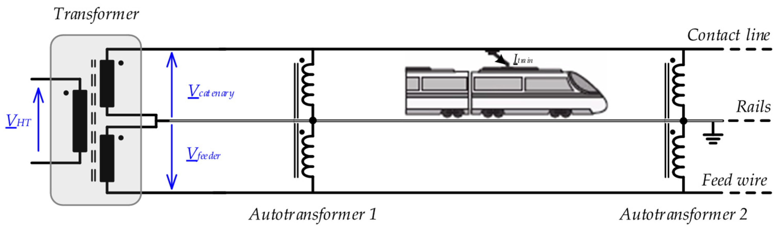
2]. The principle, as presented in
Figure 1, relies on a three-wire circuit: the substation utilizes a single-phase transformer with two secondary windings which supply the contact-line and a feed wire with voltages in phase-opposition. Autotransformers, regularly distributed along the line, boost the contact line voltage.
When a train is located between two autotransformers, at the output of a substation, the current in the rails is canceled and the electrical power absorbed by the train is transmitted by both the contact line and feed wire at a voltage of 50 kV; this halves the currents circulating in the secondary windings of the transformer. Compared to the classical two-wire 25 kV railway electrification system, the voltage drops and the Joule losses are lowered [
3,
4]. This is why the “2 × 25 kV” system is commonly used worldwide for supplying railway high-speed lines.
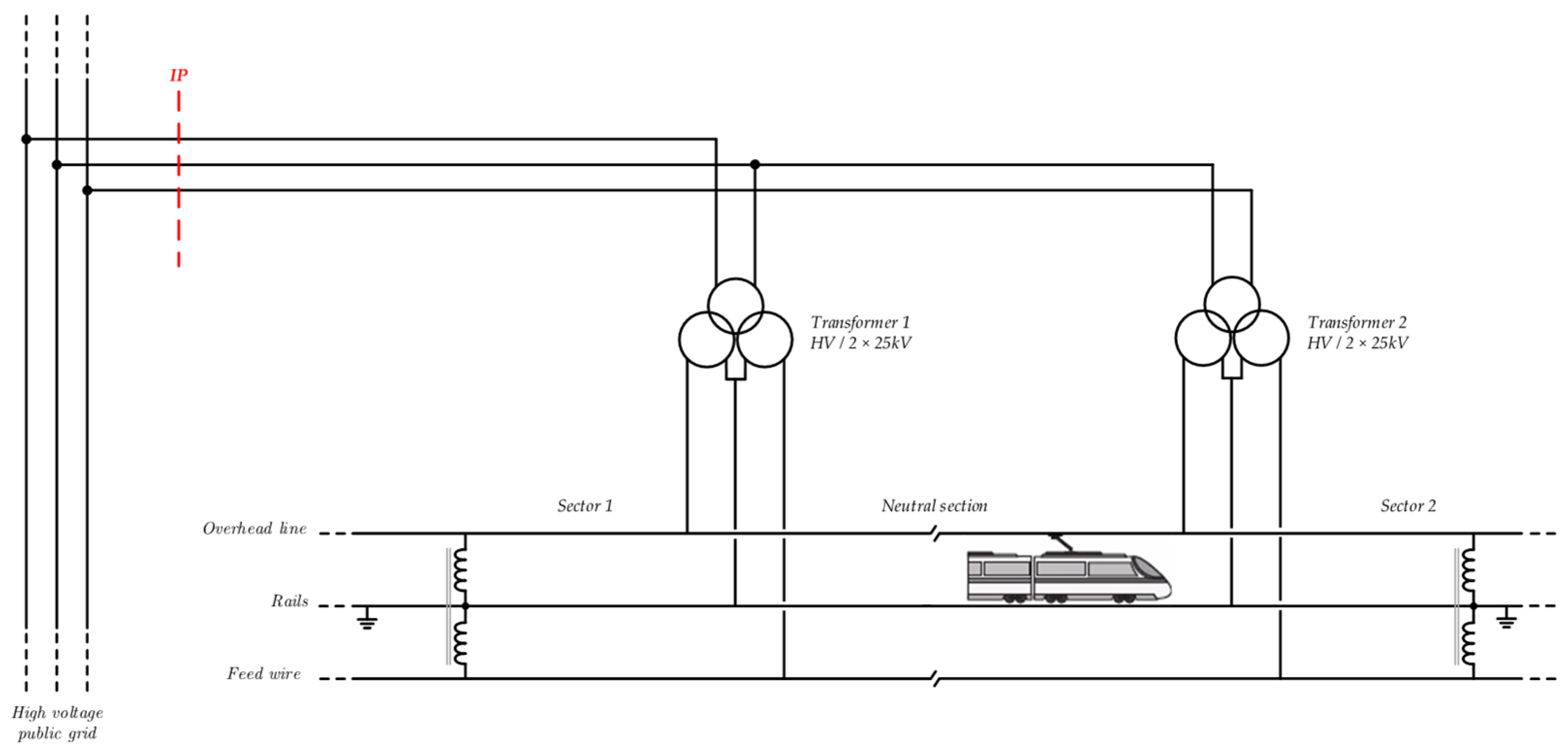
Due to the high-power supply of a high-speed line substation, it is also necessary to limit the voltage unbalance on the three-phase power grid. As shown in
Figure 2, the substation uses a V-connection scheme with two single-phase transformers supplied by two line-to-line voltages. As a result, a neutral point is created at the substation and the power supply of the railway line is divided into two sectors.
Usually, in V-connection substations, active and reactive power measurements are carried out at the secondary windings of the transformers. As a result, the primary winding currents are unknown and the calculation of the Voltage Unbalance Factor (VUF) at the Interconnection Point (IP) is an issue, as described in
Section 2. Several authors have proposed empirical formulas intended to determine the unbalance factor using the apparent powers. However, as they do not consider separately the active and reactive powers, these calculations remain inaccurate [
5,
6,
7]. Therefore, the first part of this paper presents an algorithm which allows for the line-to-line voltages at the input of the substation to be determined as a function of the power measurements provided by the remote metering system. Then, knowing the line-to-line voltages on the three-phase network, the VUF calculation is performed. A substation of the SNCF (French National Railways), located on the high-speed line between Paris and Strasbourg, has been considered as an application case. In the second part of the paper, the same algorithm is used to consider the connection of a voltage balancing system at the primary side of the substation. In all cases, the results of the calculation method are validated by simulations carried out with PLECS software [
8].
2. Calculation Method for the Voltage Unbalance Factor
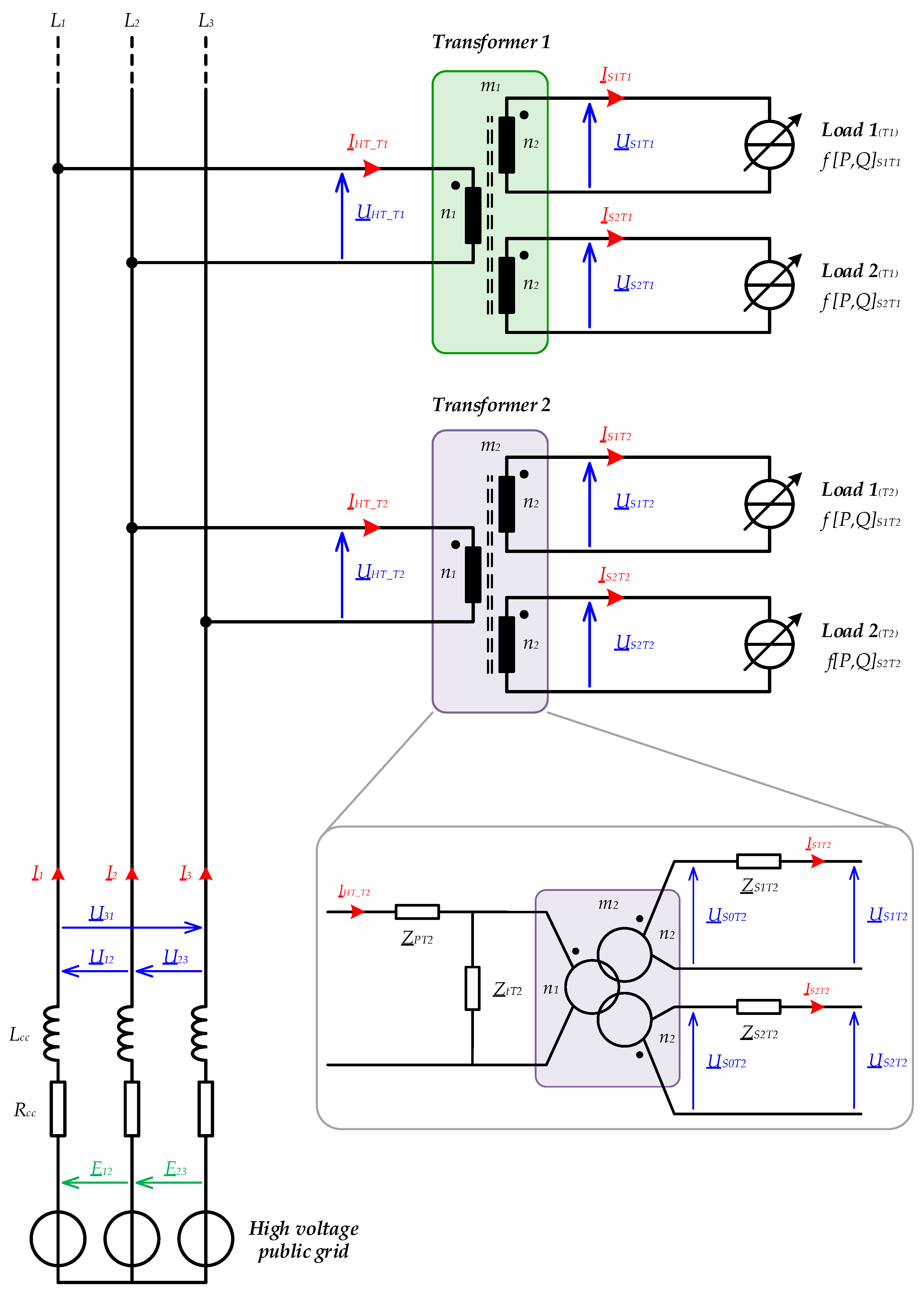
Nowadays, the SNCF traction substations are equipped with remote metering systems. At the request of the Transmission System Operator (TSO), the SNCF initiated a campaign to calculate the VUF at the connection points of traction substations. Active and reactive powers, averaged over 10 min, are stored and the number of events exceeding a 1% unbalance over a one-year period is recorded. In the future, substations whose VUFs regularly exceed 1% should be equipped with voltage balancing systems. The circuit presented in
Figure 3 constitutes the basis of this study. The high-voltage electrical transmission network is modeled as an ideal three-phase voltage source with a positive phase-sequence, associated with a series RL circuit. The parameters of this impedance are calculated from the values of the short-circuit powers given by the TSO at the interconnection points of the traction substations. The transformers’ models include the turns ratios, the magnetizing inductances, the core-loss resistances, the leakage inductances, and the resistances of each winding. These parameters are obtained from the data provided by the transformer manufacturer. The loads connected to the secondary windings of the two transformers are modeled by current sources operating at constant active and reactive powers. The powers (P and Q) correspond to those recorded by the remote metering systems.
In order to determine the line-to-line voltages at the primary side of the two transformers and then to calculate the VUF, it is first necessary to determine the currents and voltages at the secondary side. Therefore, ten unknown complex quantities have to be determined:
for Transformer 1; and
for Transformer 2.
To determine these complex quantities, it is necessary to solve a system of ten equations with ten unknowns.
For Transformer 1, the following relationship between voltages and currents can be written from the circuit of
Figure 3:
with
corresponding to the current at the primary side of Transformer 1.
For the first (“upper” in
Figure 3) secondary side of Transformer 1.
For the lower secondary side of Transformer 1.
Similarly, the expressions for Transformer 2 are:
with
corresponding to the current at the primary side of Transformer 2.
For the upper secondary side of Transformer 2.
For the lower secondary side of Transformer 2.
The phase-to-phase voltages on the primary side are defined as:
and
Relations established from Kirchhoff’s laws should be completed by the complex apparent powers at each secondary winding of the transformers. The
powers are directly calculated from the power measurements:
Then, the complex apparent powers, which are at the primary side of Transformers 1 and 2, can be calculated by Relations (9) and (10), respectively:
where
and
are the complex apparent powers for both secondary windings of Transformer 1, determined from the power measurements:
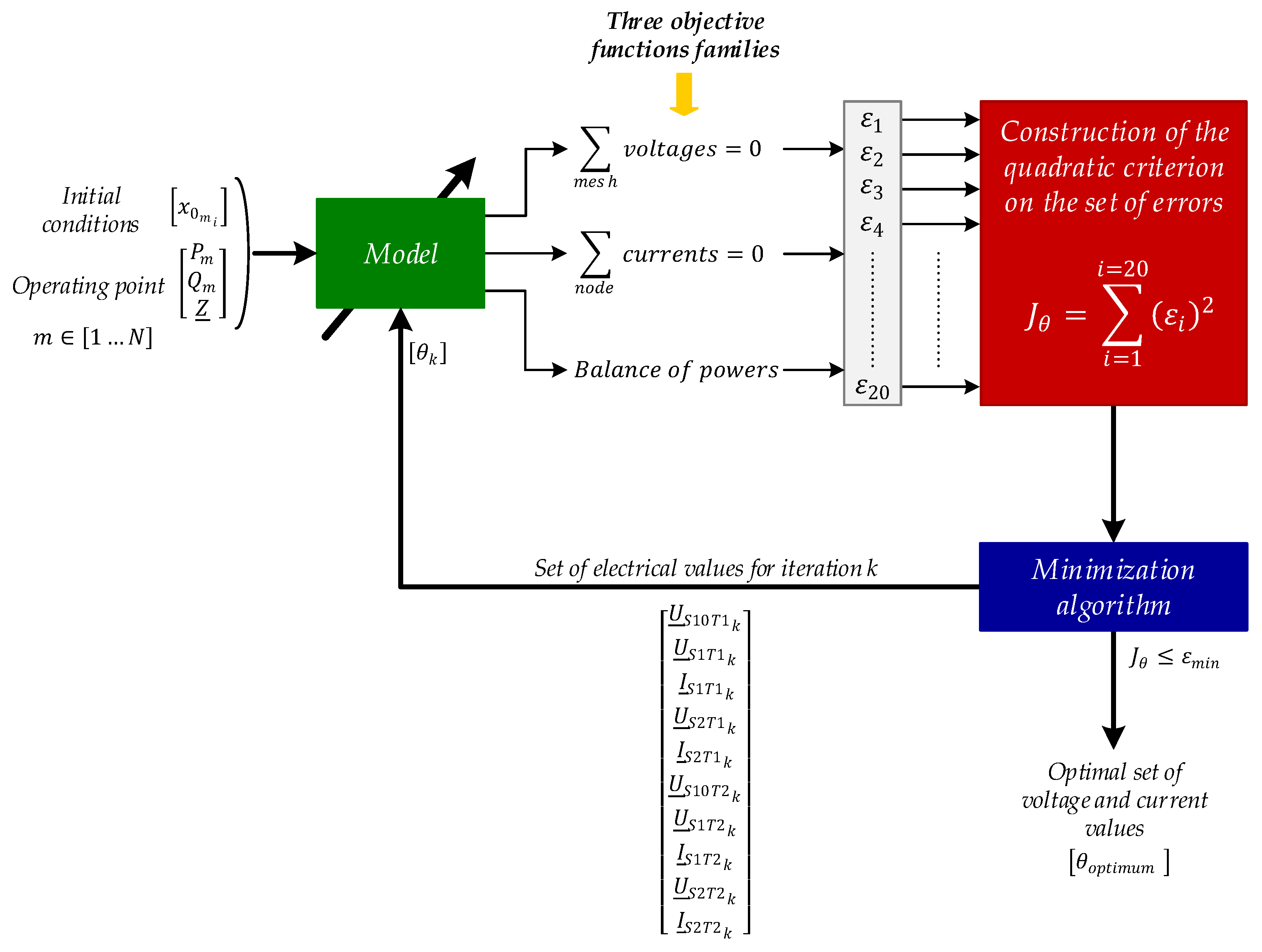
Expressions (1) to (10) correspond to a system of non-linear equations with ten complex electrical values. Indeed, the relations of the complex apparent powers involve products of voltage and current, which are unknown quantities. In this context, an iterative numerical method has been selected [
9]. The principle of the method used is illustrated by
Figure 4:
The Equations from (1) to (8) are written in a form that allows them to be solved by iterative methods: the sum of the voltages in a mesh is zero and the sum of the currents at a node is also zero. In addition, the power balance, given by Relations (9) and (10), completes the requirements of the objective functions that are used to search for the final (converged) set of voltage and current values.
2.1. Method Description
The iterative methods are based on the error calculation, which starts from an initial conditions vector
and which, by successive approaches, converges toward the solution for a given operating point. Therefore, they involve evolving the vector
to minimize an error criterion corresponding to the sum of the square of the errors. In other words, the objective of the method is to find the solution vector
such that the function
is a minimum for that presented above. It is therefore an unconstrained optimization problem such as:
This technique is based on three important choices, which are as follows.
The initial conditions: A good knowledge of the initial conditions offers a reduced computation time (lower number of iterations, allowing for faster convergence towards a solution) and a better (more accurate) convergence. In the considered case, the initial conditions are calculated by determining the powers at the output of the transformers and neglecting the voltage drops in all the series impedances.
The recurrence method: Due to the non-linear nature of the model, the Levenberg-Marquardt algorithm has been used, which is a deterministic algorithm. This means that for the same starting point, the algorithm will always give the same result. It combines two algorithms: the gradient descent method when the observed values are “far” from the optimum (the first derivative is used) and the Gauss–Newton method when the observed values are close to the optimal solution (use of the second derivative). Thus, it is possible to ensure a more robust convergence with a low resolution time.
The stopping criterion: For the practical use of such a method, it is necessary to introduce a criterion to interrupt the iterative process when the approximation is judged “satisfactory”. For that, several choices are possible:
define a maximum number of iterations;
apply a tolerance on the parameter’s increment (observation of two successive iterations); in this case, the iterations end when ;
set a tolerance on the criterion of the objective function; in this case, the iterations end when ; and
apply a tolerance on the gradient of the objective function the iterative process will then be interrupted when .
In our case, the -stopping criteria have been attributed a value of 1 × 10⁻³. This value reflects the relative tolerance accepted on the parameter’s evolution.
This method has been implemented in Matlab software and the results for a real case are presented in the next section.
2.2. Case Study
The SNCF has 47 substations with V-connections for more than 2800 km of high-speed lines. The traction substation located at “
Trois Domaines” on the high-speed line between Paris and Strasbourg is considered as an application case (
Table 1).
2.2.1. Analysis of the Algorithm Operation for one Operating Point of the Substation
Active and reactive powers measured at the secondary sides of the two transformers are given in
Table 2.
For this operating point,
Table 3 summarizes the obtained results after running the Matlab calculation routine.
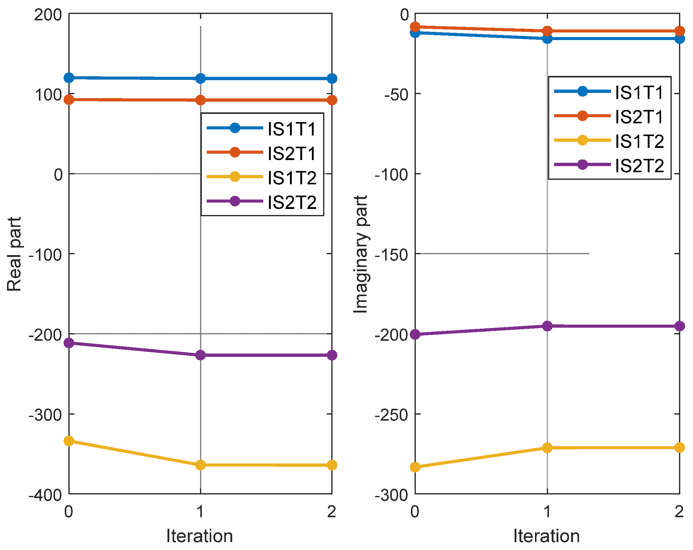
Starting from the initial conditions (Iteration 0), the algorithm finds a solution and converges in three iterations, and the stopping criterion is the relative value of the parameter’s evolution. The residual value corresponds to the square of the error of the objective function for each iteration, as follows:
The residual value of 5835 × 10−10 confirms the fact that the solver has converged to an acceptably accurate solution.
Figure 5 shows the evolution of the currents (real and imaginary parts) at the secondary side of the transformers according to the rank of the iterations. The solution found is close to the starting point, highlighting the importance of defining “good” initial conditions. From Iteration
k = 1, the values evolve slightly, which leads to a fast convergence towards the solution.
2.2.2. Calculation of Voltage Unbalance Factor
Knowing the currents at the secondary side of the transformers, it is then possible to calculate the complex values of the currents and the voltages at the primary side of the substation. Using the Fortescue method [
10,
11], the symmetrical voltage components of the positive and negative sequences of the three-phase voltage system at the interconnection point of the substation can be calculated according to Relations (13) and (14):
where the complex operator ‘a’ is defined as
.
The voltage unbalance factor, also known as the “voltage asymmetry factor”, is defined as the ratio of the negative and the positive sequence modulus:
For the considered operating point, the calculated unbalance factor is 1.55%.
2.2.3. Calculation of the VUF over a Long Period
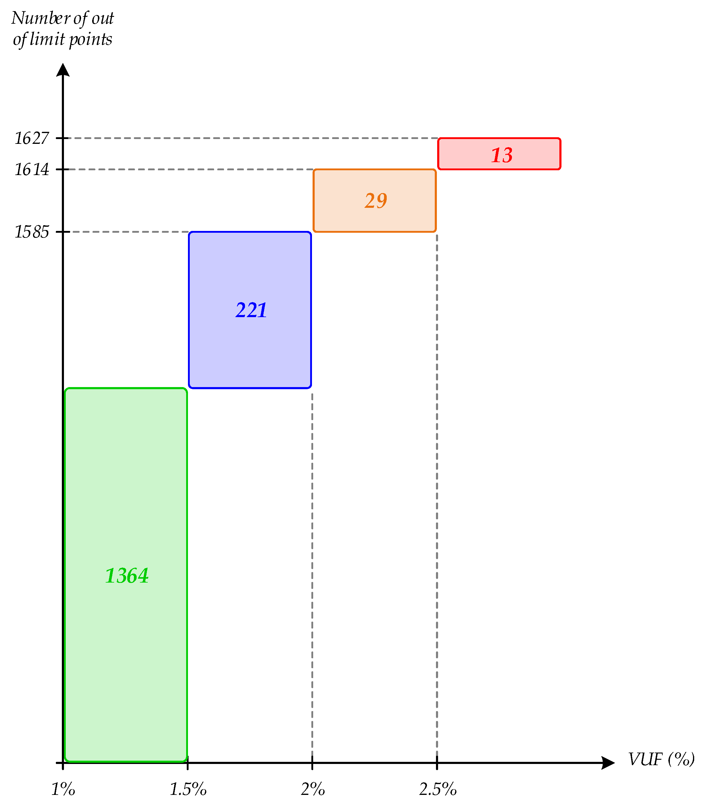
The method previously presented is used to determine the evolution of the VUF over a one-year period. The calculation is carried out from average 10 min active and reactive power data recorded by the telemetry system; that is a total of 52,560 operating points to be considered per year.
Figure 6 summarizes the number of operating points that exceed the 1% limit.
In principle, a VUF of higher than 1% is prohibited by the TSO. Nevertheless, a tolerance of a few tens of events over a year beyond this limit is accepted. Thus, the analysis of the calculation results clearly shows that the current situation is not acceptable and necessarily requires the installation of a balancing system.
3. Voltage Unbalance Calculation with the Compensation System Connected
There are mainly two voltage-balancer topologies: the voltage source inverter (VSI) [
12,
13,
14] and the High Voltage Balancing System (HVBS). The second solution relies on a Steinmetz circuit and combines both inductors and capacitors whose impedances are continuously controlled by means of AC choppers [
15]. This approach is more attractive than the inverter solution (VSI) due to lower losses in the power semiconductors and the smaller sizes of all passive components [
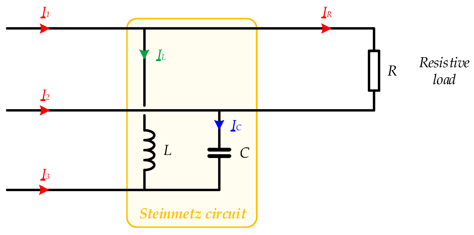
16]. C.P. Steinmetz showed that the voltage unbalance caused by unbalanced currents can be eliminated by adding a symmetrization inductor and a symmetrization capacitor to the original circuit [
17].
Figure 7 illustrates this principle for a resistive load connected across two lines. In this case, the three-phase currents
will be balanced as long as Relation (16) is satisfied.
Relation (16) can also be written in terms of the active power (P) absorbed by the resistive load and the reactive powers in both inductor L and capacitor C:
For a variable resistive load, the reactive power in inductor L and capacitor C have to be adjusted. In the case of a single-phase traction substation, the balancing circuit is composed of two branches (i.e., inductive and capacitive branches) with several AC choppers connected in series, according to
Figure 8. A three-phase transformer is used to stepdown the voltage level. The duty cycle “
α” of the AC choppers is then controlled according to Relation (18), where P is the active power absorbed by the load (i.e., the trains) and
is the maximum reactive power in the inductive and capacitive branches:
The main characteristics of this compensation system are summarized in
Table 4.
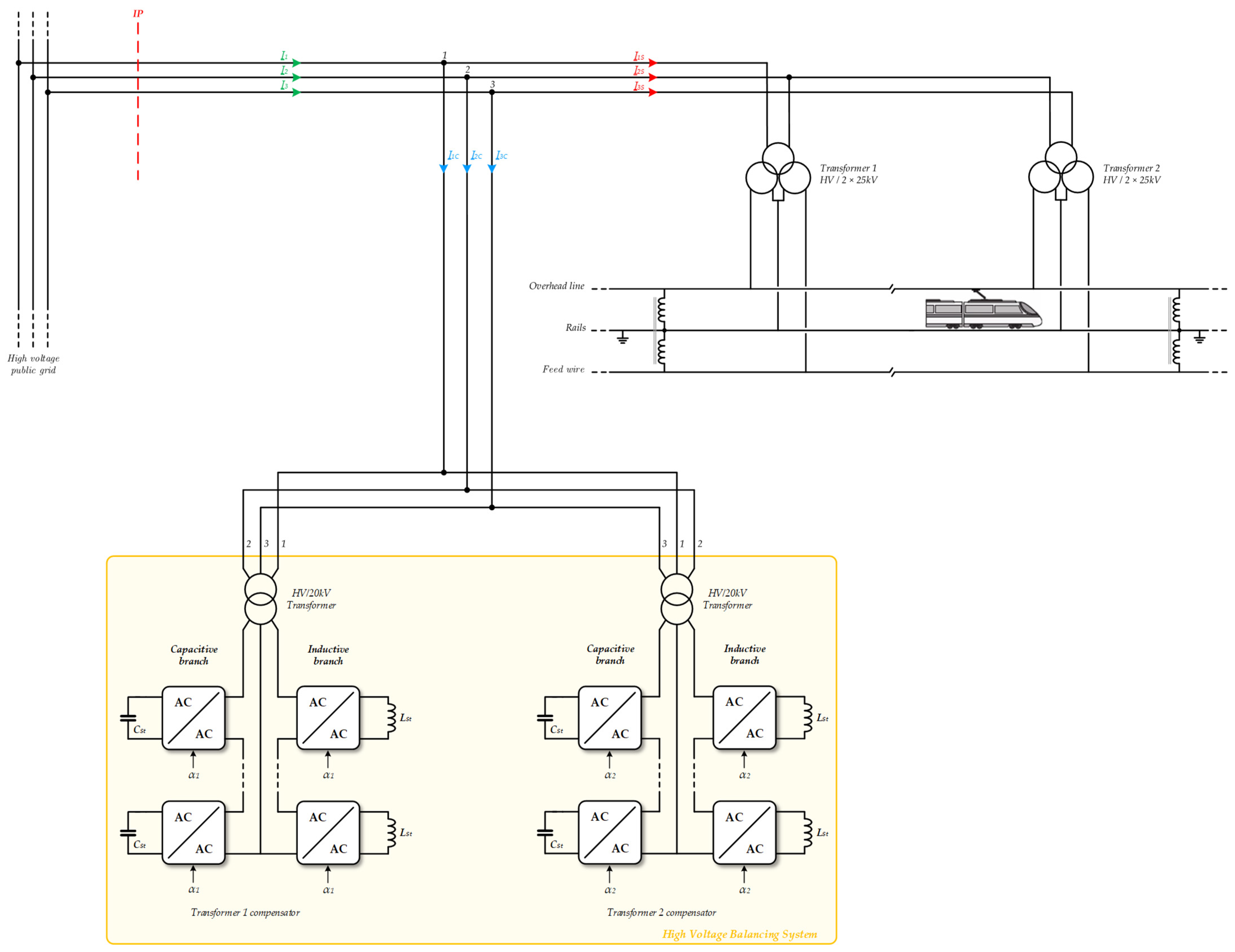
In the case of a substation using a V-connection, the High Voltage Balancing System (HVBS) has to include an active Steinmetz circuit for each transformer. The connection is given in
Figure 9.
To take into account the influence of the HVBS on the VUF, the averaged model of the AC choppers was considered. Thus, the inductive and capacitive branches are modeled by two variable complex impedances, namely
and
, which depend on the duty cycles
and
. The control of the balancing system is very simple: the duty cycle of each active Steinmetz circuit is fixed according to the total active power delivered by the corresponding transformers:
and
Figure 10 illustrates the final circuit, which is considered to establish the new equations of the electrical circuit.
With this new configuration, Equations (7) and (8), which express the phase-to-phase voltages, become:
and
These two expressions form a system of two equations with two unknown variables that can be solved numerically and thus the calculation of VUF is carried out in the same way as in
Section 2.2.2.
According to the power consumption of the traction substation located at “
Trois Domaines”, the calculation results showed that it is necessary to install two HVBS in parallel in order to bring the VUF to a maximum value of around 1%.
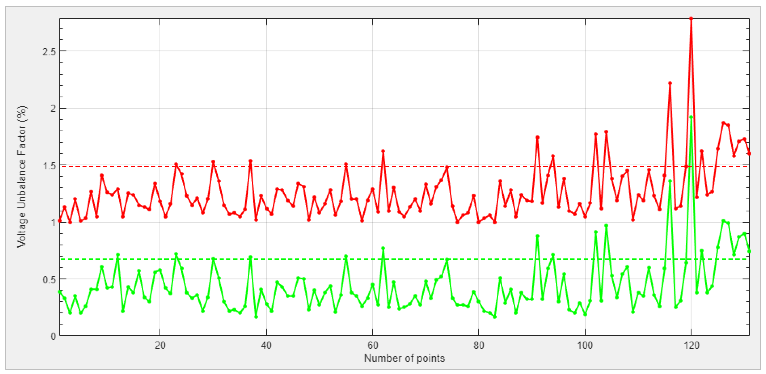
Figure 11 gives the result of an analysis over a one-month period considering the measurements of active and reactive powers averaged over 10 min, which represents 4320 points. Before compensation, 131 points are beyond 1% and only three points after compensation. Considering a period of one year, 1627 operating points out of 52,560 were over the 1% limit. With two HVBS connected in parallel, only 69 operating points exceed 1% and the averaged value of VUF over one year is 0.53%, which is perfectly tolerable for the TSO.
The entire circuit, including the two HVBSs, was implemented in PLECS software using the averaged model of the AC choppers [
18]. To illustrate the calculation results, simulations were performed for the operating point presented in
Table 2.
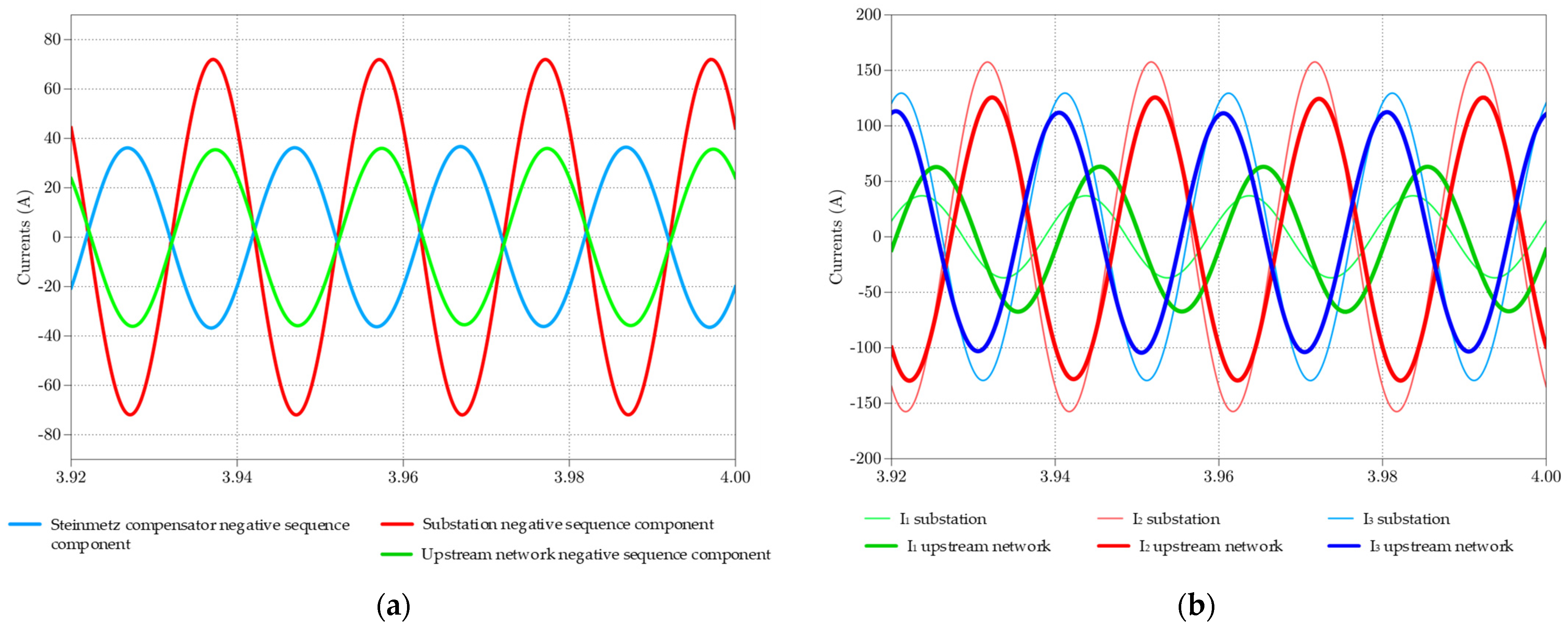
Figure 12a shows the negative sequence components of the three-phase currents at different points of the circuit. The HVBS absorbs a negative sequence current in phase-opposition with that of the substation. The negative sequence current at the point of interconnection is halved, which is enough to bring the VUF back below 1%.
Figure 12b shows the three-phase current waveforms at the substation and at the interconnection point. Specifically, these waveforms highlight the fact that the HVBS rebalances the magnitude and the phase of the three-phase currents at the interconnection point.
The simulations show the effect of the HVBS on the VUF.
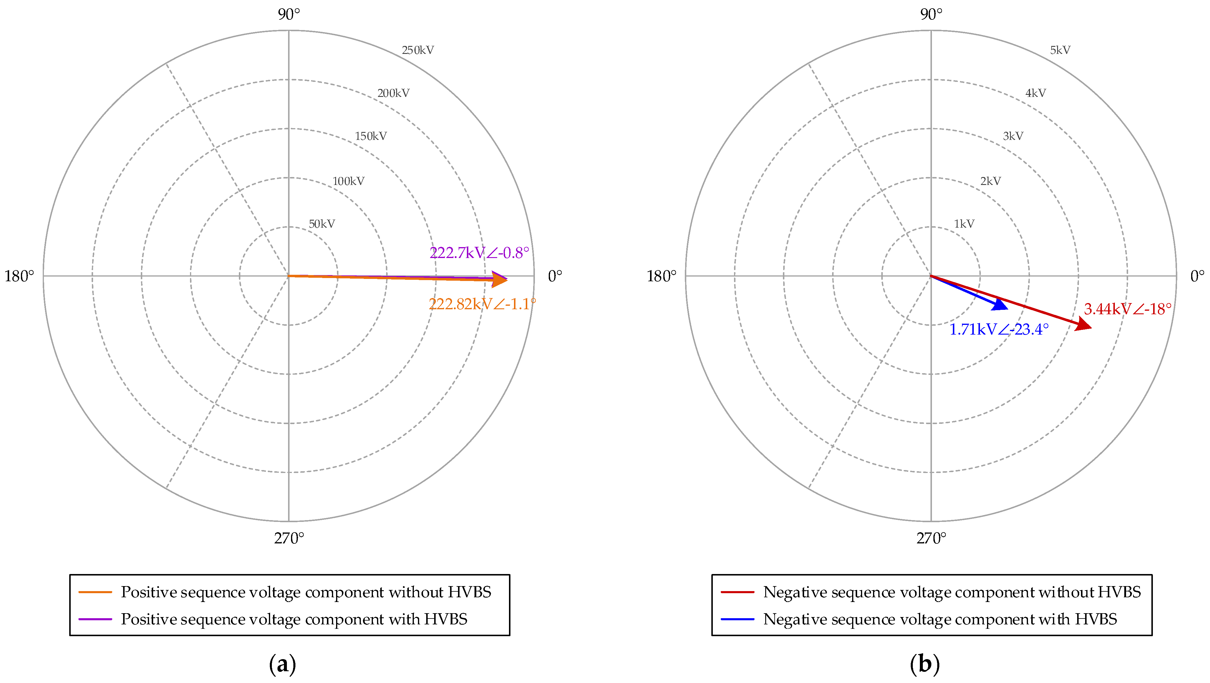
Figure 13 shows, in the complex plane, the positive and negative sequence voltages before and after compensation. Phase-to-phase voltage
is the reference of
. The negative sequence voltage is decreased by 50% and the VUF goes from 1.55% to 0.77%. The simulation results also confirm the validity of the calculation method proposed in
Section 2. As a comparison, considering the same operating point, the empirical formulas presented in papers [
5,
6] give, respectively, a value of the unbalance factor of 1.34% and 1.37%, i.e., a relative error of 13.5% and 11.7%. It should be noted that these formulas cannot be used with a balancing system.
4. Conclusions
The calculation method presented in this paper makes it possible to accurately determine, from power telemetry, the VUF for traction substations with V-connection schemes. The processing of the 52,560 points corresponding to a year’s operation was carried out in 1.5 h on a desktop computer. It moves away from empirical methods which are still used in practice.
A complete modelling of the substation, including the transformers and the upstream electric network, was proposed.
An iterative algorithm was proposed for solving the circuit equations. Once all the electrical quantities have been calculated, it is possible to determine the VUF at the connection point of the substation.
In
Section 3, the circuit equations were easily modified to include a balancing system based on a Steinmetz circuit controlled by AC choppers and the same iterative algorithm was used.
In all cases, the results obtained from the iterative calculation method were compared with simulations carried out with PLECS power electronic circuit simulation software. The error on all voltage and current quantities always remains as less than 1%. Finally, the calculation tool presented in this paper is essential for a railway network operator. On the one hand, it allows for the determination of the VUF from the power consumption of a substation and, on the other hand, it makes it possible to analyze the effect of installing a balancing system based on a Steinmetz circuit controlled by AC choppers.


