Boundary-Aware Salient Object Detection in Optical Remote-Sensing Images

Abstract

Different from the traditional natural scene images, optical remote-sensing images (RSIs) suffer from diverse imaging orientations, cluttered backgrounds, and various scene types. Therefore, the object-detection methods salient to optical RSIs require effective localization and segmentation to deal with complex scenarios, especially small targets, serious occlusion, and multiple targets. However, the existing models’ experimental results are incapable of distinguishing salient objects and backgrounds using clear boundaries. To tackle this problem, we introduce boundary information to perform salient object detection in optical RSIs. Specifically, we first combine the encoder’s low-level and high-level features (i.e., abundant local spatial and semantic information) via a feature-interaction operation, yielding boundary information. Then, the boundary cues are introduced into each decoder block, where the decoder features are directed to focus more on the boundary details and objects simultaneously. In this way, we can generate high-quality saliency maps which can highlight salient objects from optical RSIs completely and accurately. Extensive experiments are performed on a public dataset (i.e., ORSSD dataset), and the experimental results demonstrate the effectiveness of our model when compared with the cutting-edge saliency models.

1. Introduction

Human vision systems tend to focus more on prominent areas in images, which is the visual attention mechanism, with many efforts made to design various methods to highlight salient objects in images or videos [1,2].

Formally, salient object detection is employed to automatically highlight the most visually distinctive regions in a scene [2], and has been applied to many research fields, such as object detection [3], image segmentation [4], image quality assessment [5], visual categorization [6], and medical image processing [7], to name a few.

Over the last twenty years, many saliency models have been designed [1,8]. The early efforts mainly focus on hand-crafted features, including the prior heuristic-based efforts [9,10,11] and the traditional machine-learning-based methods [12,13,14]. With the rapid development of deep-learning technologies, many deep-learning-based saliency models [15,16,17,18,19,20,21] have significantly improved the performance of saliency detection. Among the existing deep-learning-based models, some models [16,17,18,19] attempt to introduce edge information into their networks to provide precise boundary details for inference results. The current saliency models are obviously applicable to traditional RGB images (natural scenes) [22], RGB-T images [23], RGB-D images [24], light-field images [25], and optical remote-sensing images [26,27]. Among these, the saliency detection of optical remote-sensing images has gained increasing attention, because it has been widely employed in a variety of domains, including military, agriculture, and disaster relief.

However, there is a significant difference between the traditional natural-scene images and optical remote-sensing images. Salient objects in traditional natural-scene images are usually with high-contrast, a single object, and a prior center. In contrast, the objects in optical RSIs are usually of diverse types, various scales, and different orientations. Meanwhile, the optical RSIs have low contrast between salient objects and background. In addition, optical RSIs are usually photographed by high-altitude aircrafts or satellites. Recently, there have been many efforts devoted to this research field [26,28,29,30,31]. However, their performance degrades to some degree when dealing with some complex scenes.

Motivated by the aforementioned descriptions, we propose an innovative boundary-aware saliency model to detect salient objects in optical RSIs, as shown in Figure 1. Our model is built using an encoder–decoder architecture, and we focus on the extraction and usage of salient boundaries. Concretely, our model contains three modules, including the feature-extraction module (i.e., encoder), the edge module, and the feature-integration module (i.e., decoder). Particularly, our model first extracts salient boundaries via an edge module. Similarly to [16], the edge module simultaneously incorporates low-level and high-level deep features to generate boundary cues, where the low-level features convey spatial details and high-level deep features provide rich semantic information. In contrast to [16], our edge module also investigates the interaction effect [19] of salient boundaries and salient objects, which further elevates the boundary features and object features. Here, different from [19], we do not adopt stack modules to iteratively refine deep features. Instead, the salient boundaries are endowed with position information about salient objects, which promotes the completeness of saliency inference. Then, we pass on the boundary information to each decoding process, in which the salient boundary progressively refines the salient reasoning. In this way, we can obtain high-quality saliency maps to highlight salient regions in optical RSIs.

Overall, the main contributions of the proposed network can be presented as follows:

• We propose a novel boundary-aware saliency model for salient object detection, in which our model tries to introduce the salient boundaries to precisely segment the salient objects from optical RSIs.
• We propose an effective edge module to provide boundary information for saliency detection, where boundary cues and object features are enhanced by the interaction between low-level spatial features and high-level semantic features.
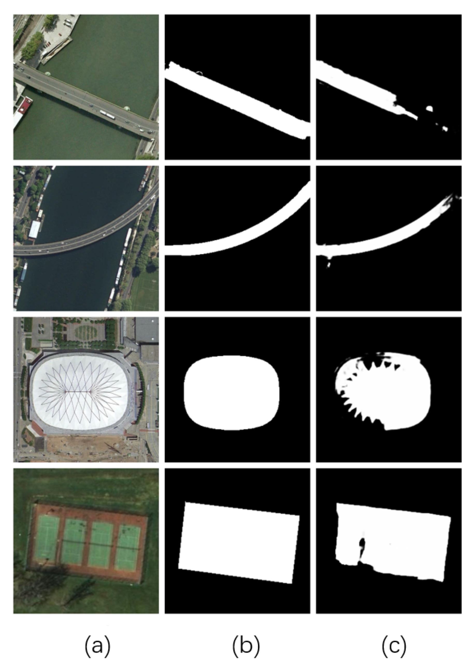
• Extensive experiments are performed on the public dataset ORSSD, and the results show that our model performs better than the state-of-the-art saliency models, which demonstrates the effectiveness of the proposed model.

The remaining of this paper is organized as follows. The related works are reviewed in Section 2. Section 3 gives a detailed introduction to the proposed saliency model. The experimental results and the analyses are detailed in Section 4. Finally, we draw a conclusion for this paper in Section 5.

2. Related Works

In recent years, we have seen significant advances in the research on salient object detection. Particularly, from the heuristic prior-based models [2,9,13] to the deep-learning-based models [17,18,19], significant efforts for salient object detection have been made. Meanwhile, due to the imaging method and image complexity, there is considerable difference between salient object detection in optical RSIs and salient object detection targeting natural-scene images. Therefore, this section mainly gives a brief review of the two different tasks.

2.1. Saliency Detection of Nature-Scene Images

Early efforts were usually constructed based on heuristic priors such as center prior, contrast prior, morphology prior, background prior, and so on. The pioneering work was proposed by Itti et al. [2], where the center-surround difference is designed to compute saliency scores using color, orientation, and intensity features. Subsequently, Cheng et al. [9] proposed a global contrast-based saliency model which gives a good segmentation for the prominent objects in natural images. In [32], Wei et al. paid more attention to the background rather than salient objects, and proposed a geodesic saliency model by exploiting boundary and connectivity priors of natural images. After that, machine-learning algorithms have been devoted to saliency models. For example, Liu et al. [33] attempted to aggregate multiple feature-based saliency maps using the conditional random forest. In [34], Huang et al. exploited multiple-instances learning algorithms to compute the saliency values of different regions. In [3], the Adaboost algorithm was adopted to fuse various hand-crafted feature-based saliency maps. Abdusalomov et al. [35] presented a unique saliency cutting method, which exploits local adaptive thresholding to generate four regions from a given saliency map.

Recently, deep-learning technologies have achieved remarkable progress, and they have also been applied to the saliency detection task. For example, Hou et al. [15] inserted short connections into the skip-layer structures of holistically nested edge detectors which effectively improve the quality of saliency inference results. In [22], Deng et al. proposed a recurrent residual refinement network to perform saliency detection, in which the residual refinement blocks learn the complementary saliency information by using low-level and high-level features. Qin et al. [36] designed a two-level nested U structure to capture more context information from different sizes of receptive fields, for which the rise in the network depth does not increase the memory and computation cost. In [37], Wang et al. exploited the recurrent fully convolutional networks to integrate saliency prior cues for more precise saliency prediction. In [38], Liu et al. designed a pooling-based structure to reduce the aliasing effect, where the global guidance module and the feature-aggregation module are deployed to progressively refine the high-level semantic information. Meanwhile, the authors also employed edge cues to sharpen the boundary details of salient objects. Similarly, in [16,17], the edge information was implicity and explicitly used to give a good depiction of the salient edges, respectively.

2.2. Saliency Detection of Optical Remote-Scene Images

Remarkable progress has been made in the saliency models aiming at natural-scene images, and lots of methods are proposed to enhance the effect of optical RSIs. In [28], Zhao et al. proposed a sparsity-guided saliency model which used bayesian theory to combine global and background features. In [29], the structure tensor and background contrast are employed to generate superpixel feature maps which are fused into the final pixel-level saliency map. In [39], Li et al. proposed a two-step building extraction method from remote-sensing images by fusing saliency information, of which the rooftops are more likely to attract visual attention than surrounding objects. In [40], the fully convolutional network is utilized to address the issue of inshore ship detection, where the deep layer of the network conducts detection and the shallow layer supplements with precise localization. In [30], Zhang et al. constructed a saliency-oriented active contour model, where the contour information is adopted to assist object detection. In [41], a self-adaptive multiple-feature fusion method is employed to explore the internal connection in optical RSIs, where the dual-tree complex wavelet transform is used to obtain the texture features. In [42], Liu et al. tried to adopt an unsupervised method to solve the oil-tank detection problem using the color Markov chain. In [43], a multi-level ship-detection method is proposed to detect various types of offshore ships using all possible imaging variations. Recently, in [26,27], the authors articulated further concerns regarding the integration of multi-level deep features, which can effectively highlight salient objects in optical RSIs.

Though the existing saliency models targeting natural-scene images have achieved satisfactory performance, it is inappropriate to extend the existing models to optical RSIs directly. The reason behind this lies in the differences between the two kinds of images. In addition, the existing saliency models targeting optical RSIs suffer from low-quality boundary details due to the neglecting of edge information. Therefore, in this paper, we attempt to integrate the edge cues into the entire network.

3. The Proposed Method

This part first gives an overview of the proposed saliency model in Section 3.1. Then, the detailed description of the proposed saliency model is presented in the following sections. Section 3.2 details the feature extraction (i.e., encoder). Section 3.3 presents the edge module. Section 3.4 provides the details of feature integration (i.e., decoder). Lastly, the training and implementation details will be outlined in Section 3.5.

3.1. Overall Architecture

The overall architecture of our model is shown in Figure 1. The main part of our model is constructed based on a U-shape structure. Given an optical remote-sensing image $\mathbf{I}$, we first feed it into the encoder part to extract multi-level features ${\left\{{\mathbf{F}}_i\right\}}_{i=1}^6$. Then, the feature ${\mathbf{F}}_6$ will feed into a bridge module “Conv-bridge" to further capture effective global semantic information ${\mathbf{F}}_6^B$. After that, we use the decoder to aggregate the multi-level deep features $\{{\left\{{\mathbf{F}}_i\right\}}_{i=1}^5,{\mathbf{F}}_6^B\}$, yielding the final saliency map $\mathbf{S}$. During the decoding process, to give a precise saliency inference, we introduce the edge information into the decoding process, where the edge feature ${\mathbf{F}}^E$ generated by the edge module combines with the multi-level deep features $\{{\mathbf{F}}_2,{\mathbf{F}}_5\}$.

3.2. Feature Extraction

Salient objects in optical RSIs vary different sizes. This phenomenon will degrade the performance of saliency models. Meanwhile, we find that many efforts [17,36] have sufficiently extracted and fused multi-level deep features including low-level information and high-level information. Inspired by SegNet [36] and BASNet [17], our saliency model, shown in Figure 1, is designed as an encoder–decoder structure with multi-level feature extraction. Meanwhile, following the deeply supervised efforts [16,44], the side outputs of our decoder are also supervised by the ground truth. The encoder of our model consists of six convolution blocks, where the first four blocks are the same as ResNet-34 [45]. The fifth block and the sixth block are all composed of three basic residual blocks [45] with 512 filters after a non-overlapping max pooling layer (size = 2). Based on the encoder, we can obtain six deep features ${\left\{{\mathbf{F}}_i\right\}}_{i=1}^6$. In addition, referring to BASNet [17], we also add a bridge module after the sixth convolutional block, which endows our model with more representative semantic features. The bridge module consists of three convolution layers with 512 dilated (dilation=2) 3×3 convolutional layers, and each convolution layer is followed by a batch-normalization (BN) layer and a ReLU activation function. Based on the bridge module, we can generate a more effective semantic feature ${\mathbf{F}}_6^B$. Following this encoder architecture, we can obtain the six levels of deep features $\{{\left\{{\mathbf{F}}_i\right\}}_{i=1}^5,{\mathbf{F}}_6^B\}$.

3.3. Edge Module

Edge information is useful for optimizing segmentation [16]. Many saliency models [16,17,38] have introduced edge information to conduct salient object detection, which gives accurate boundary details for saliency maps. Although the existing methods use edge information to guide the inference network, the extraction of edge features is not efficient. Furthermore, the existing models do not give sufficient usage of edge information. Therefore, we propose a novel edge module, which has two streams, as shown in Figure 1.

Specifically, the feature ${\mathbf{F}}_2$ from the second convolutional block and the feature ${\mathbf{F}}_5$ from the fifth convolutional block are first processed by convolutional layers, which can be written as

$$\begin{array}{c}\hfill \left\{\begin{array}{c}\hfill {\mathbf{F}}_2^C=Conv\left({\mathbf{F}}_2\right)\\ \hfill {\mathbf{F}}_5^C=Conv\left({\mathbf{F}}_5\right)\end{array},\right.\end{array}$$

(1)

where $Conv$ means convolutional block.

Then, the convolutional block results ${\mathbf{F}}_2^C$ and ${\mathbf{F}}_5^C$ are used to generate the saliency and edge maps. Firstly, the feature ${\mathbf{F}}_2^C$ first concatenates with the feature ${\mathbf{F}}_5^C$, and then the concatenated feature is processed by a convolutional layer. In addition, the output of the convolutional layer and ${\mathbf{F}}_5^C$ are further combined via an element-wise summation. Lastly, we predict a saliency map ${\mathbf{S}}^{*}$ on the combined feature via convolutional layers. This process can be defined as follows

$${\mathbf{S}}^{*}=\delta \left(Conv(Conv\left([{\mathbf{F}}_2^C,{\mathbf{F}}_5^C]\right)+{\mathbf{F}}_5^C)\right),$$

(2)

where $\delta$ denotes the sigmoid activation function.

In addition, the features ${\mathbf{F}}_2^C$ and ${\mathbf{F}}_5^C$ are first combined in an element-wise multiplication fashion, and then the multiplication result is processed by a convolutional layer. The fused feature further combines the feature ${\mathbf{F}}_2^C$. Finally, we predict the edge $\mathbf{E}$ from the fused feature via convolutional layers, which are further supervised by the salient edge maps. The entire process can be defined as

$$\mathbf{E}=\delta \left(Conv(Conv\left([{\mathbf{F}}_2^C\odot {\mathbf{F}}_5^C]\right)+{\mathbf{F}}_5^C)\right).$$

(3)

Therefore, in our edge module, the edge information not only contains spatial details but is also endowed with semantic information about salient objects. This is beneficial for the following decoding process (i.e., feature integration).

3.4. Feature Integration

Many saliency inference networks [17,46] adopt the encoder–decoder architecture to conduct salient object detection, which progressively recovers the spatial details of saliency maps and achieves promising results. Inspired by this, we also adopt the encoder–decoder architecture while introducing the edge information. Here, our decoder contains six decoder blocks, namely, Decoderi ($i=1,\cdots ,6$). Each decoder block consists of three convolutional blocks, where each convolutional block contains a convolutional layer, a batch-normalization (BN) layer, and a ReLU layer. During the decoding process, the input of each decoder block is the decoder feature ${\left\{{\mathbf{F}}_i^D\right\}}_{i=2}^6$ from the previous decoder block and the encoder feature ${\left\{{\mathbf{F}}_i\right\}}_{i=1}^5$ from the current-level encoder block. Meanwhile, to endow our model with accurate spatial details, we combine the edge information ${\mathbf{F}}^E$ with each encoder feature, and the enhanced encoder feature will take part in the decoding process. Therefore, we define each decoding process as follows

$${\mathbf{F}}_i^D=Conv\left([{\mathbf{F}}_{i+1}^D,{\mathbf{F}}_i,{\mathbf{F}}^E]\right).$$

(4)

In this way, we can obtain six levels of decoder features, namely, ${\left\{{\mathbf{F}}_i^D\right\}}_{i=1}^6$. After that, we combine all decoder features and the edge cues, which can be written as

$${\mathbf{F}}_D=[{\mathbf{F}}_1^D,{\mathbf{F}}_2^D,{\mathbf{F}}_3^D,{\mathbf{F}}_4^D,{\mathbf{F}}_5^D,{\mathbf{F}}_6^D,{\mathbf{F}}^E],$$

(5)

where ${\mathbf{F}}_D$ is the fused feature. Based on ${\mathbf{F}}_D$, we deploy a 3×3 convolutional layer and sigmoid activation function to generate the final saliency map $\mathbf{S}$. The entire process can be defined as

$$\mathbf{S}=\delta \left(Conv\left({\mathbf{F}}_D\right)\right).$$

(6)

3.5. Model Learning and Implementation

Deep supervision has been successfully adopted by many vision tasks [36,47], where the deep supervision can promote the training process and improve the performance of saliency models [44,48]. Inspired by the existing saliency object-detection models [17,38,44], we give deep supervision for six decoder blocks using the hybrid loss [17]. The total loss l of our model can be denoted as:

$$l=\sum _i(l_{bce}^i+l_{IoU}^i+l_{ssim}^i+l_{bce}^{e,i}).$$

(7)

where $l_{bce}^i$, $l_{IoU}^i$ and $l_{ssim}^i$ denote the BCE loss, IoU loss and SSIM loss of the ith sample. $l_{bce}^{e,i}$ is used to compute the edge loss.

To train our model, we adopt the same training set as LV-Net [26], where 600 images selected from the ORSSD dataset [26] are used for the training set and the remaining 200 images are treated as the testing set. Furthermore, to train the proposed model, the training set is augmented by performing rotation with angles 90, 180 and 270 and conducting flipping on the rotated images. Following this, the training set contains 4800 samples.

We implemented our model with Pytorch on a PC with an Intel i7-6700 CPU, 32GB RAM, and a NVIDIA GeForce RTX2080Ti (with 11GB memory). We set our epoch number and batch size to 200 and 4, respectively. The input images were resized to 256 × 256. Our optimizer is Adam, where the initial learning rate lr = ${10}^{-3}$, betas = (0.9, 0.999), eps = ${10}^{-8}$, and weight decay = 0.

4. Experimental Results

This section first presents the ORSSD datasets and evaluation metrics in Section 4.1. Then, in Section 4.2, we compare our model with the state-of-the-art optical RSIs saliency models from the perspective of quantitative and qualitative views. Lastly, the detailed ablation studies are shown in Section 4.3.

4.1. Datasets and Evaluation Metrics

To comprehensively validate our model, we adopt the public challenging optical RSIs dataset, namely, ORSSD [26]. Concretely, the ORSSD dataset contains 600 images with pixel-wise annotations. The images have diverse resolutions such as 256 × 256, 300 × 300, and 800 × 600. They contain lots of scenes, such as house, airplane, car, ship, bridge, sea, river, and bay, etc.

To quantitatively compare all the models, we employed four evaluation metrics, S-measure (S) [49], max F-measure (maxF), max E-measure (maxE) [50] and mean absolute error (MAE), to evaluate the performance of all models.

To perform a subjective comparison of all models, we employed a method of subjective comparison. Concretely, we first randomly selected some images and their corresponding ground truths. Then, we visually presented the saliency maps of our model and other state-of-the-art models.

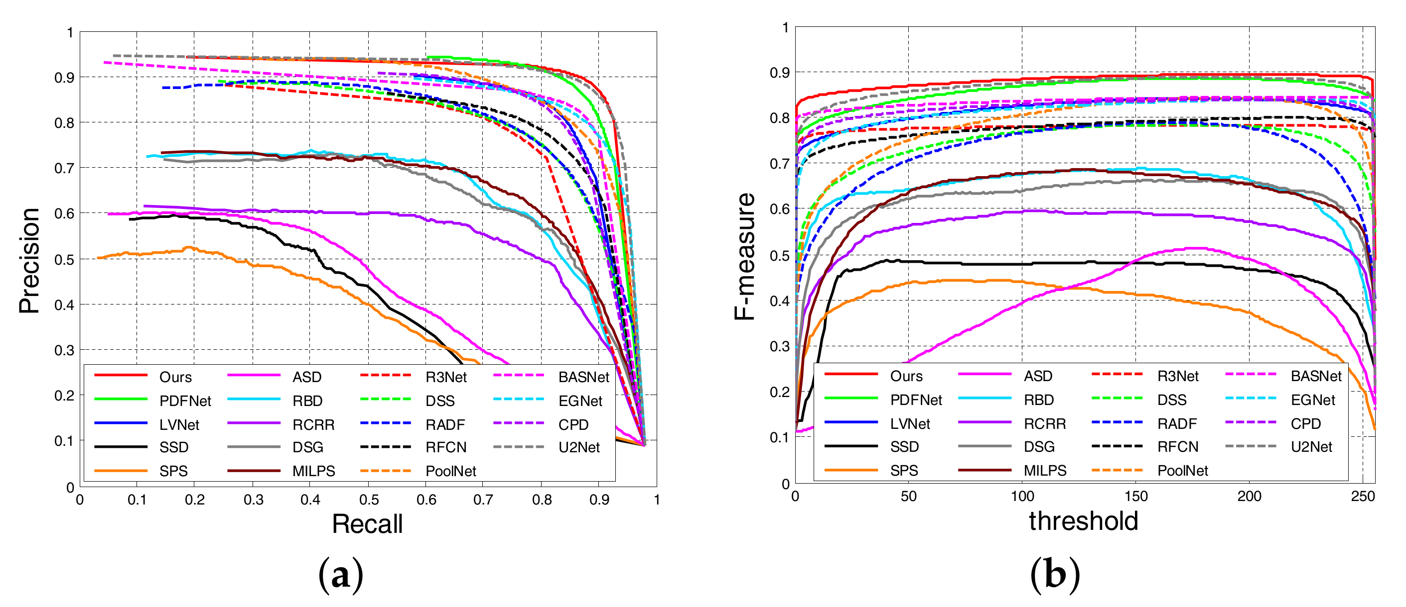
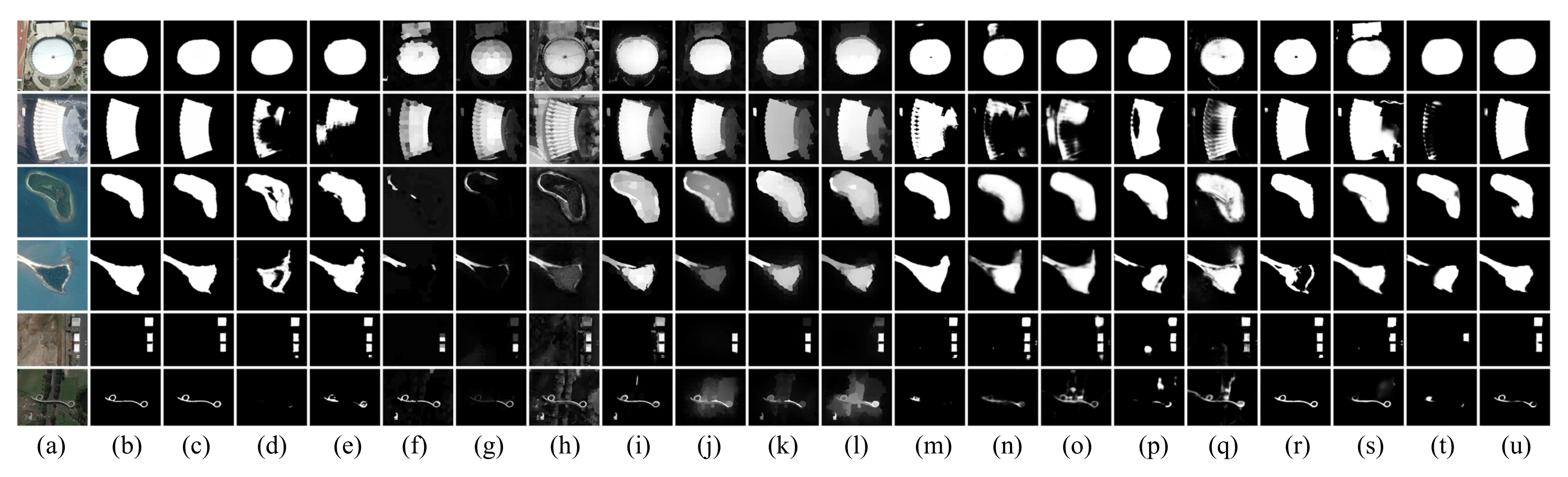
4.2. Comparison with the State of the Art

To validate the performance of our model, we drew a comparison between our model and 19 state-of-the-art saliency models containing five optical RSIs saliency models (PDFNet [27], LVNet [26], SSD [28], SPS [29], ASD [30]); four unsupervised saliency models majoring in natural-scene images (RBD [11], RCRR [14], DSG [51], MILPS [34]); and 10 deep-learning-based saliency models targeting natural-scene images (R3Net [22], DSS [15], RADF [52], RFCN [37], PoolNet [38], BASNet [17], EGNet [16], CPD [18], SCRN [19], U2Net [36]) on the ORSSD dataset. Meanwhile, for a fair comparison, we retrained the existing deep-learning-based models by running the source codes or obtaining the results provided by the authors. Next, we show the quantitative and qualitative comparisons, successively.

Table 1. Quantitative comparison results of S-measure, max F-measure, max E-measure, and MAE on the ORSSD dataset. Here, “↑” (“↓”) means that the larger (smaller) the better. The best three results in each row are marked in red, green, and blue, respectively.

	ORSSD Dataset
	$S\uparrow$	$F_{\beta }\uparrow$	$E_{\beta }\uparrow$	$MAE\downarrow$
PDFNet [27]	0.9112	0.8726	0.9608	0.0149
LVNet[26]	0.8815	0.8263	0.9456	0.0207
SSD[28]	0.5838	0.4460	0.7052	0.1126
SPS[29]	0.5758	0.3820	0.6472	0.1233
ASD[30]	0.5477	0.4701	0.7448	0.2119
RBD [11]	0.7662	0.6579	0.8501	0.0626
RCRR [14]	0.6849	0.5591	0.7651	0.1277
DSG [51]	0.7195	0.6238	0.7912	0.1041
MILPS [34]	0.7361	0.6519	0.8265	0.0913
R3Net [22]	0.8141	0.7456	0.8913	0.0399
DSS [15]	0.8262	0.7467	0.8860	0.0363
RADF [52]	0.8259	0.7619	0.9130	0.0382
RFCN [37]	0.8437	0.7742	0.9157	0.0293
PoolNet [38]	0.8551	0.8229	0.9368	0.0293
BASNet [17]	0.8963	0.8282	0.9346	0.0204
EGNet [16]	0.8774	0.8187	0.9165	0.0308
CPD [18]	0.8627	0.8033	0.9115	0.0297
SCRN [19]	0.9061	0.8846	0.9647	0.0157
U2Net [36]	0.9162	0.8738	0.9539	0.0166
Ours	0.9233	0.8786	0.9581	0.0120

reports the quantitative results of our model and the 19 latest methods on the benchmark dataset. According to the evaluation results, it can be seen that our model performs best. Specifically, the performance of our model is better than the top-two models including SCRN, PDFNet in terms of S-measure and MAE, and our model performs slightly lower than SCRN in terms of F-measure and E-measure. In addition, we also present the PR curves and F-measure curves of different models in Figure 2. It can be clearly seen that our model outperforms other models.

In addition, Figure 3 shows the qualitative analysis of different models. It can be seen that our model can more completely highlight irregular objects and multiple objects. For example, in Figure 3f,g, the large object is not completely detected, whereas the saliency map is incomplete. In stark contrast, our model can give an accurate saliency prediction, and the object is completely highlighted. In Figure 3m,q,r, the saliency maps cannot completely highlight salient objects. Similarly, in Figure 3, the existing models cannot highlight the fifth row of objects, whereas the saliency maps only detect parts of salient objects. Meanwhile, we can find that our model, Figure 3c, can completely and accurately highlight salient objects. This is mainly a benefit of the edge module of our model, which provides accurate edge information for salient objects.

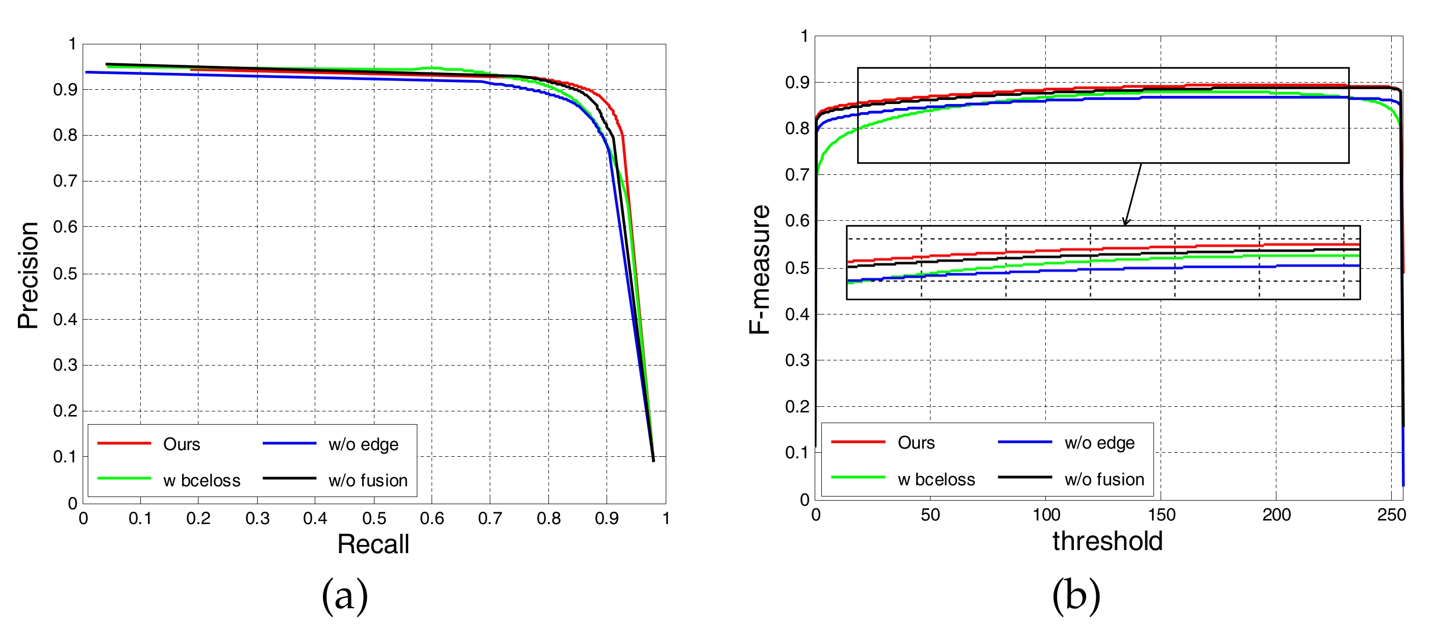
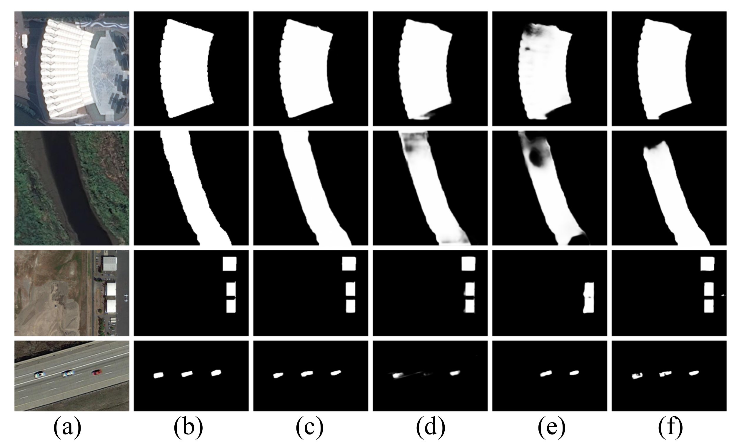
4.3. Ablation Studies

This section profoundly analyzes some important components of our model through quantitative and qualitative comparisons. Specifically, the crucial components of our model include the edge module and the fusion module. Our model without edge information is denoted as “w/o Edge”. Our model does not fuse the side outputs of the decoder, and performs saliency inference on the first decoder block, which is denoted as “w/o Fusion”. In addition, we also explore the BCE loss in the supervision of saliency maps, and, thus, we remove the BCE loss in the hybrid loss, which is marked as “w/o bceloss”.

According to the quantitative comparison results shown in

Table 2. Ablation analysis on ORSSD dataset. The best result is marked in boldface. ↑ and ↓ represent smaller and larger is better.

Model	$\mathit{S}-\mathit{measure}\uparrow$	$\mathit{MAE}\downarrow$	$\mathit{maxE}\uparrow$	$\mathit{maxF}\uparrow$
$w/obceloss$	0.8980	0.0182	0.9482	0.8612
$w/oEdge$	0.9054	0.0160	0.9501	0.8523
$w/oFusion$	0.9142	0.0149	0.9514	0.8690
Ours	0.9233	0.0120	0.9581	0.8786

and Figure 4, we can find that our model outperforms the three variations including w/o Edge, w/o Fusion, and w/o bceloss in terms of S-measure, max F-measure, max E-measure, and MAE. From the qualitative comparison results shown in Figure 5, we can find that the Edge module, Fusion module, and BCE loss can effectively improve the performance of our model to a certain extent. This clearly demonstrates the effectiveness of the three components in our model.

4.4. Failure Cases and Analysis

According to the aforementioned descriptions, the proposed model can accurately highlight salient objects in optical RSIs. However, our model is still incapable of generating satisfactory results when dealing with the different scales of salient objects shown in Figure 6. For instance, the two examples in the first and second rows of Figure 6 present two salient objects, i.e., bridges and tiny vehicles. As presented in Figure 6c, our model falsely highlights the background regions around the salient objects. It can be seen that the predicted saliency maps cannot completely highlight salient objects when dealing with the tiny white vehicles. For the bottom two examples in Figure 6a, a roof with patterned lines and a stadium with shadows are where the contrast between salient objects and background is low. As presented in Figure 6c, our model is incapable of highlighting salient objects. Therefore, we can conclude that the scene with different-sized salient objects are still challenging for our model. To address this issue, we should pay more attention to the design of the effective integration methods for multi-level deep features, providing more discriminative representations for salient objects.

5. Conclusions

This paper introduces the boundary information into our model for salient object detection in optical RSIs. Concretely, the edge module is first designed to acquire the edge cues. Here, we combine the low-level feature and the high-level feature to interactively obtain the edge features. Then, we endow the generated multi-level deep features with the edge cues, using the edge information to enhance the decoding process. This can direct the features and give more options for salient regions in optical RSIs. Following this, we can obtain high-quality saliency maps which can highlight salient objects from optical RSIs entirely and accurately. Experiments are conducted on the public dataset, and the comprehensive comparison results show that our model performs better than the state-of-the-art models. In our future work, we will address more concerns on designing more effective saliency models targeting optical RSIs, which will be endowed with powerful characterization ability for salient objects and equipped with an effective feature fusion module.

References

1. Borji, A.; Cheng, M.M.; Hou, Q.; Jiang, H.; Li, J. Salient Object Detection: A Survey. Comput. Vis. Pattern Recognit. 2014, 5, 117–150. [Google Scholar] [CrossRef] [Green Version]
2. Itti, L.; Koch, C.; Niebur, E. A model of saliency-based visual attention for rapid scene analysis. IEEE Trans. Pattern Anal. Mach. Intell. 1998, 20, 1254–1259. [Google Scholar] [CrossRef] [Green Version]
3. Zhou, X.; Liu, Z.; Sun, G.; Ye, L.; Wang, X. Improving saliency detection via multiple kernel boosting and adaptive fusion. IEEE Signal Process. Lett. 2016, 23, 517–521. [Google Scholar] [CrossRef]
4. Chen, L.C.; Papandreou, G.; Kokkinos, I.; Murphy, K.; Yuille, A.L. Deeplab: Semantic image segmentation with deep convolutional nets, atrous convolution, and fully connected crfs. IEEE Trans. Pattern Anal. Mach. Intell. 2017, 40, 834–848. [Google Scholar] [CrossRef] [PubMed] [Green Version]
5. Wang, X.; Ma, L.; Kwong, S.; Zhou, Y. Quaternion representation based visual saliency for stereoscopic image quality assessment. Signal Process. 2018, 145, 202–213. [Google Scholar] [CrossRef]
6. Han, J.; Yao, X.; Cheng, G.; Feng, X.; Xu, D. P-CNN: Part-Based Convolutional Neural Networks for Fine-Grained Visual Categorization. IEEE Trans. Pattern Anal. Mach. Intell. 2020, 44, 579–590. [Google Scholar] [CrossRef]
7. Khosravan, N.; Celik, H.; Turkbey, B.; Cheng, R.; McCreedy, E.; McAuliffe, M.; Bednarova, S.; Jones, E.; Chen, X.; Choyke, P.; et al. Gaze2Segment: A pilot study for integrating eye-tracking technology into medical image segmentation. In Medical Computer Vision and Bayesian and Graphical Models for Biomedical Imaging; Springer: Berlin/Heidelberg, Germany, 2016; pp. 94–104. [Google Scholar]
8. Wang, W.; Lai, Q.; Fu, H.; Shen, J.; Ling, H.; Yang, R. Salient object detection in the deep learning era: An in-depth survey. IEEE Trans. Pattern Anal. Mach. Intell. 2021, 44, 3239–3259. [Google Scholar] [CrossRef]
9. Cheng, M.M.; Zhang, G.X.; Mitra, N.J.; Huang, X.; Hu, S.M. Global contrast based salient region detection. In Proceedings of the IEEE Conference on Computer Vision and Pattern Recognition (CVPR), Colorado Springs, CO, USA, 20–25 June 2011; IEEE: New York, NY, USA, 2011; pp. 409–416. [Google Scholar]
10. Perazzi, F.; Krähenbühl, P.; Pritch, Y.; Hornung, A. Saliency filters: Contrast based filtering for salient region detection. In Proceedings of the IEEE Conference on Computer Vision and Pattern Recognition (CVPR), Providence, RI, USA, 16–21 June 2012; IEEE: New York, NY, USA, 2012; pp. 733–740. [Google Scholar]
11. Zhu, W.; Liang, S.; Wei, Y.; Sun, J. Saliency optimization from robust background detection. In Proceedings of the IEEE Conference on Computer Vision and Pattern Recognition (CVPR), Columbus, OH, USA, 23–28 June 2014; IEEE: New York, NY, USA, 2014; pp. 2814–2821. [Google Scholar]
12. Tong, N.; Lu, H.; Ruan, X.; Yang, M.H. Salient object detection via bootstrap learning. In Proceedings of the IEEE Conference on Computer Vision and Pattern Recognition (CVPR), Columbus, OH, USA, 23–28 June 2014; IEEE: New York, NY, USA, 2015; pp. 1884–1892. [Google Scholar]
13. Jiang, H.; Wang, J.; Yuan, Z.; Wu, Y.; Zheng, N.; Li, S. Salient object detection: A discriminative regional feature integration approach. In Proceedings of the IEEE Conference on Computer Vision and Pattern Recognition (CVPR), Portland, OR, USA, 23–28 June 2013; IEEE: New York, NY, USA, 2013; pp. 2083–2090. [Google Scholar]
14. Yuan, Y.; Li, C.; Kim, J.; Cai, W.; Feng, D.D. Reversion correction and regularized random walk ranking for saliency detection. IEEE Trans. Image Process. 2017, 27, 1311–1322. [Google Scholar] [CrossRef] [Green Version]
15. Hou, Q.; Cheng, M.M.; Hu, X.; Borji, A.; Tu, Z.; Torr, P.H. Deeply supervised salient object detection with short connections. In Proceedings of the IEEE Conference on Computer Vision and Pattern Recognition (CVPR), Honolulu, HI, USA, 21–26 July 2017; IEEE: New York, NY, USA, 2017; pp. 3203–3212. [Google Scholar]
16. Zhao, J.X.; Liu, J.J.; Fan, D.P.; Cao, Y.; Yang, J.; Cheng, M.M. EGNet: Edge guidance network for salient object detection. In Proceedings of the International Conference on Computer Vision (ICCV), Seoul, Republic of Korea, 27 October–2 November 2019; IEEE: New York, NY, USA, 2019; pp. 8779–8788. [Google Scholar]
17. Qin, X.; Zhang, Z.; Huang, C.; Gao, C.; Dehghan, M.; Jagersand, M. Basnet: Boundary-aware salient object detection. In Proceedings of the IEEE Conference on Computer Vision and Pattern Recognition (CVPR), Long Beach, CA, USA, 15–20 June 2019; IEEE: New York, NY, USA, 2019; pp. 7479–7489. [Google Scholar]
18. Wu, Z.; Su, L.; Huang, Q. Cascaded partial decoder for fast and accurate salient object detection. In Proceedings of the IEEE Conference on Computer Vision and Pattern Recognition (CVPR), Long Beach, CA, USA, 15–20 June 2019; IEEE: New York, NY, USA, 2019; pp. 3907–3916. [Google Scholar]
19. Wu, Z.; Su, L.; Huang, Q. Stacked cross refinement network for edge-aware salient object detection. In Proceedings of the International Conference on Computer Vision (ICCV), Seoul, Republic of Korea, 27 October–2 November 2019; IEEE: New York, NY, USA, 2019; pp. 7264–7273. [Google Scholar]
20. Chen, C.; Wei, J.; Peng, C.; Zhang, W.; Qin, H. Improved Saliency Detection in RGB-D Images Using Two-Phase Depth Estimation and Selective Deep Fusion. IEEE Trans. Image Process. 2020, 29, 4296–4307. [Google Scholar] [CrossRef]
21. Chen, C.; Wang, G.; Peng, C.; Fang, Y.; Zhang, D.; Qin, H. Exploring Rich and Efficient Spatial Temporal Interactions for Real-Time Video Salient Object Detection. IEEE Trans. Image Process. 2021, 30, 3995–4007. [Google Scholar] [CrossRef]
22. Deng, Z.; Hu, X.; Zhu, L.; Xu, X.; Qin, J.; Han, G.; Heng, P.A. R3net: Recurrent residual refinement network for saliency detection. In Proceedings of the 27th International Joint Conference on Artificial Intelligence (IJCAI), Stockholm, Sweden, 13–19 July 2018; AAAI Press: Menlo Park, CA, USA, 2018; pp. 684–690. [Google Scholar]
23. Tu, Z.; Xia, T.; Li, C.; Wang, X.; Ma, Y.; Tang, J. RGB-T Image Saliency Detection via Collaborative Graph Learning. IEEE Trans. Multimed. 2020, 22, 160–173. [Google Scholar] [CrossRef] [Green Version]
24. Cong, R.; Lei, J.; Fu, H.; Huang, Q.; Cao, X.; Hou, C. Co-saliency Detection for RGBD Images Based on Multi-constraint Feature Matching and Cross Label Propagation. IEEE Trans. Image Process. 2017, 27, 568–579. [Google Scholar] [CrossRef] [PubMed] [Green Version]
25. Piao, Y.; Li, X.; Zhang, M.; Yu, J.; Lu, H. Saliency Detection via Depth-Induced Cellular Automata on Light Field. IEEE Trans. Image Process. 2020, 29, 1879–1889. [Google Scholar] [CrossRef] [PubMed]
26. Li, C.; Cong, R.; Hou, J.; Zhang, S.; Qian, Y.; Kwong, S. Nested network with two-stream pyramid for salient object detection in optical remote sensing images. IEEE Trans. Geosci. Remote Sens. 2019, 57, 9156–9166. [Google Scholar] [CrossRef] [Green Version]
27. Li, C.; Cong, R.; Guo, C.; Li, H.; Zhang, C.; Zheng, F.; Zhao, Y. A parallel down-up fusion network for salient object detection in optical remote sensing images. Neurocomputing 2020, 415, 411–420. [Google Scholar] [CrossRef]
28. Zhao, D.; Wang, J.; Shi, J.; Jiang, Z. Sparsity-guided saliency detection for remote sensing images. J. Appl. Remote Sens. 2015, 9, 095055. [Google Scholar] [CrossRef] [Green Version]
29. Ma, L.; Du, B.; Chen, H.; Soomro, N.Q. Region-of-interest detection via superpixel-to-pixel saliency analysis for remote sensing image. IEEE Geosci. Remote Sens. Lett. 2016, 13, 1752–1756. [Google Scholar] [CrossRef]
30. Zhang, Q.; Zhang, L.; Shi, W.; Liu, Y. Airport extraction via complementary saliency analysis and saliency-oriented active contour model. IEEE Geosci. Remote Sens. Lett. 2018, 15, 1085–1089. [Google Scholar] [CrossRef]
31. Zhang, Q.; Cong, R.; Li, C.; Cheng, M.M.; Fang, Y.; Cao, X.; Zhao, Y.; Kwong, S. Dense Attention Fluid Network for Salient Object Detection in Optical Remote Sensing Images. IEEE Trans. Image Process. 2020, 30, 1305–1317. [Google Scholar] [CrossRef]
32. Wei, Y.; Wen, F.; Zhu, W.; Sun, J. Geodesic saliency using background priors. In Proceedings of the European Conference on Computer Vision, Florence, Italy, 7–13 October 2012; Springer: Berlin/Heidelberg, Germany, 2012; pp. 29–42. [Google Scholar]
33. Liu, T.; Yuan, Z.; Sun, J.; Wang, J.; Zheng, N.; Tang, X.; Shum, H.Y. Learning to detect a salient object. IEEE Trans. Pattern Anal. Mach. Intell. 2010, 33, 353–367. [Google Scholar]
34. Huang, F.; Qi, J.; Lu, H.; Zhang, L.; Ruan, X. Salient object detection via multiple instance learning. IEEE Trans. Image Process. 2017, 26, 1911–1922. [Google Scholar] [CrossRef] [PubMed]
35. Abdusalomov, A.; Mukhiddinov, M.; Djuraev, O.; Khamdamov, U.; Whangbo, T.K. Automatic salient object extraction based on locally adaptive thresholding to generate tactile graphics. Appl. Sci. 2020, 10, 3350. [Google Scholar] [CrossRef]
36. Qin, X.; Zhang, Z.; Huang, C.; Dehghan, M.; Zaiane, O.R.; Jagersand, M. U2-Net: Going deeper with nested U-structure for salient object detection. Pattern Recognit. 2020, 106, 107404. [Google Scholar] [CrossRef]
37. Wang, L.; Wang, L.; Lu, H.; Zhang, P.; Ruan, X. Salient object detection with recurrent fully convolutional networks. IEEE Trans. Pattern Anal. Mach. Intell. 2018, 41, 1734–1746. [Google Scholar] [CrossRef]
38. Liu, J.J.; Hou, Q.; Cheng, M.M.; Feng, J.; Jiang, J. A simple pooling-based design for real-time salient object detection. In Proceedings of the IEEE Conference on Computer Vision and Pattern Recognition (CVPR), Long Beach, CA, USA, 15–20 June 2019; IEEE: New York, NY, USA, 2019; pp. 3917–3926. [Google Scholar]
39. Li, E.; Xu, S.; Meng, W.; Zhang, X. Building extraction from remotely sensed images by integrating saliency cue. IEEE J. Sel. Top. Appl. Earth Obs. Remote Sens. 2016, 10, 906–919. [Google Scholar] [CrossRef]
40. Lin, H.; Shi, Z.; Zou, Z. Fully convolutional network with task partitioning for inshore ship detection in optical remote sensing images. IEEE Geosci. Remote Sens. Lett. 2017, 14, 1665–1669. [Google Scholar] [CrossRef]
41. Zhang, L.; Liu, Y.; Zhang, J. Saliency detection based on self-adaptive multiple feature fusion for remote sensing images. Int. J. Remote Sens. 2019, 40, 8270–8297. [Google Scholar] [CrossRef]
42. Liu, Z.; Zhao, D.; Shi, Z.; Jiang, Z. Unsupervised Saliency Model with Color Markov Chain for Oil Tank Detection. Remote Sens. 2019, 11, 1089. [Google Scholar] [CrossRef] [Green Version]
43. Dong, C.; Liu, J.; Xu, F.; Liu, C. Ship Detection from Optical Remote Sensing Images Using Multi-Scale Analysis and Fourier HOG Descriptor. Remote Sens. 2019, 11, 1529. [Google Scholar] [CrossRef] [Green Version]
44. Liu, Y.; Cheng, M.M.; Zhang, X.Y.; Nie, G.Y.; Wang, M. DNA: Deeply supervised nonlinear aggregation for salient object detection. arXiv 2021, arXiv:1903.12476. [Google Scholar] [CrossRef]
45. He, K.; Zhang, X.; Ren, S.; Sun, J. Deep residual learning for image recognition. In Proceedings of the IEEE Conference on Computer Vision and Pattern Recognition (CVPR), Las Vegas, NA, USA, 27–30 June 2016; IEEE: New York, NY, USA, 2016; pp. 770–778. [Google Scholar]
46. Ronneberger, O.; Fischer, P.; Brox, T. U-Net: Convolutional Networks for Biomedical Image Segmentation. Med. Image Comput. Comput. Assist. Interv. 2015, 9351, 234–241. [Google Scholar]
47. Liu, N.; Han, J.; Yang, M.H. PiCANet: Learning Pixel-wise Contextual Attention for Saliency Detection. Comput. Vis. Pattern Recognit. 2017, 3089–3098. [Google Scholar]
48. Xie, S.; Tu, Z. Holistically-Nested Edge Detection. Int. J. Comput. Vis. 2015, 1395–1403. [Google Scholar]
49. Fan, D.P.; Cheng, M.M.; Liu, Y.; Li, T.; Borji, A. Structure-measure: A new way to evaluate foreground maps. In Proceedings of the International Conference on Computer Vision (ICCV), Venice, Italy, 22–29 October 2017; pp. 4548–4557. [Google Scholar]
50. Fan, D.P.; Gong, C.; Cao, Y.; Ren, B.; Cheng, M.M.; Borji, A. Enhanced-alignment Measure for Binary Foreground Map Evaluation. In Proceedings of the 27th International Joint Conference on Artificial Intelligence (IJCAI), Stockholm, Sweden, 13–19 July 2018; AAAI Press: Menlo Park, CA, USA, 2018; pp. 698–704. [Google Scholar]
51. Zhou, L.; Yang, Z.; Zhou, Z.; Hu, D. Salient region detection using diffusion process on a two-layer sparse graph. IEEE Trans. Image Process. 2017, 26, 5882–5894. [Google Scholar] [CrossRef]
52. Hu, X.; Zhu, L.; Qin, J.; Fu, C.W.; Heng, P.A. Recurrently aggregating deep features for salient object detection. In Proceedings of the Thirty-second AAAI conference on Artificial Intelligence (AAAI), New Orleans, LA, USA, 2–7 February 2018. [Google Scholar]
Figure 1. Illustration of the proposed saliency model.
Electronics 11 04200 g001
Figure 2. (Better viewed in color) quantitative evaluation of different saliency models: (a) P-R curves of different methods of the ORSSD dataset, and (b) F-measure curves of different methods of the ORSSD dataset.
Electronics 11 04200 g002
Figure 3. Visualization comparison of different optical RSI saliency models on several challenging scenes. (a): RGB, (b): GT, (c): Ours, (d): PDFNet, (e): LVNet, (f): RBD, (g): RCRR, (h): DSG, (i): MILPS, (j): SSD, (k): SPS, (l): ASD, (m): R3Net, (n): DSS, (o): RADF, (p): RFCN, (q): PoolNet (r): BASNet (s): EGNet (t): CPD, (u): U2Net.
Electronics 11 04200 g003
Figure 4. (better viewed in color) Quantitative evaluation of our network and ablation network: (a) P-R curves, and (b) F-measure curves.
Electronics 11 04200 g004
Figure 5. Qualitative Visual results of ablation analysis. (a): RGB, (b): GT, (c): Ours, (d): w/o Edge, (e): w/o Fusion, (f): w/o bceloss.
Electronics 11 04200 g005
Figure 6. Some failure examples. (a) Optical RSIs. (b) Ground truth. (c) Saliency maps generated by our model.
Electronics 11 04200 g006