UFace: An Unsupervised Deep Learning Face Verification System

Abstract

Deep convolutional neural networks are often used for image verification but require large amounts of labeled training data, which are not always available. To address this problem, an unsupervised deep learning face verification system, called UFace, is proposed here. It starts by selecting from large unlabeled data the k most similar and k most dissimilar images to a given face image and uses them for training. UFace is implemented using methods of the autoencoder and Siamese network; the latter is used in all comparisons as its performance is better. Unlike in typical deep neural network training, UFace computes the loss function k times for similar images and k times for dissimilar images for each input image. UFace’s performance is evaluated using four benchmark face verification datasets: Labeled Faces in the Wild (LFW), YouTube Faces (YTF), Cross-age LFW (CALFW) and Celebrities in Frontal Profile in the Wild (CFP-FP). UFace with the Siamese network achieved accuracies of 99.40%, 96.04%, 95.12% and 97.89%, respectively, on the four datasets. These results are comparable with the state-of-the-art methods, such as ArcFace, GroupFace and MegaFace. The biggest advantage of UFace is that it uses much less training data and does not require labeled data.

1. Introduction

Face recognition is a technology that identifies or verifies a person from an image or video [1]. Generally, face verification is used to access an application, system or service. The task is to compare a given face to another face and verify whether it is a match. In other words, given any two face images, the face verification algorithm decides if they are of the same person or not. Unlike other verification methods such as using passwords or fingerprints, biometric face verification uses dynamic patterns that make this approach one of the safest and most effective ones. Face recognition is also used in forensics and transaction authentication.

Deep neural networks have been successfully used in different applications such as speaker verification [2,3] and image recognition [4,5]. In addition to artificial neural networks, spiking neural networks have been successfully used for image recognition [6,7].

It was shown that using deep neural networks for face verification [8,9,10,11,12,13,14,15,16,17,18,19,20,21] significantly improved accuracy when compared with other face verification systems [22,23,24,25,26,27]. The Facenet [8] face verification system was developed by Google; it used a Siamese network [28] trained on a labeled dataset with 200 M faces. It achieved an accuracy of over 98% on LFW [29] and over 95% on YTF [30], two benchmark face verification datasets. To achieve that result, it used a huge labeled dataset, with 200 M faces, for training. DeepFace [9] was developed by Meta. It used 3D face modeling and a nine-layer network with about 120 million parameters and was trained on 4.4 M labeled face images. On the LFW dataset, it achieved an accuracy of over 97%. DeepFace was extended in [18] and, by using much more training data—over 500 M faces—improved its performance on LFW to over 98%. Another face verification system, VGG Face, was developed at Oxford [10], used 37 convolutional layers and was trained on 2.6 M labeled face images. It achieved accuracies comparable to Facenet and DeepFace on LFW, and over 97% on the YTF dataset. In [15], another face verification system was proposed using marginal loss, which was trained on a 4 M labeled dataset, and achieved an accuracy of over 99% on LFW and over 95% on YTF. ArcFace [16] used an additive angular margin loss and obtained over 99% accuracy on LFW, over 98% on both YTF and CFP-FP, and over 95% on CALFW. GroupFace [19] used multiple group-aware representations and achieved over 99%, 97%, 96% and 98% on the LFW, YTF, CALFW and CFP-FP datasets, respectively. However, both ArcFace and GroupFace required labeled training data of 5.8 M samples. MegaFace [31] deployed a magnitude-aware margin on ArcFace loss to improve intra-class compactness and achieved over 96% and 98% on CALFW and CFP-FP datasets, respectively. CurricularFace [13] used an adaptive curriculum learning loss and achieved over 99% on LFW, over 96% on CALFW and 98% on CFP-FP datasets. Both CurricularFace and MegaFace required about 3.8 M labeled training data. MDCNN [32] is composed of two advanced deep learning neural network models and achieved over 99% and 94% on the LFW and YTF datasets, respectively, using a 1 M labeled training dataset. PSO AlexNet TL [33] used transfer learning and achieved an accuracy of over 99% on the LFW dataset. Ref. [34] used data augmentation and achieved over 99% and 96% on the LFW and YTF datasets, respectively.

Semi-supervised learning methods with deep neural networks use two main approaches: (1) consistency regularization-based methods [35] and (2) proxy label-based methods [36]. The consistency regularization-based methods use a regularization term in the objective function to enable consistency while training on a large amount of unlabeled data; this constrains model predictions to be invariant to input noise. Ref. [35] developed an Unsupervised Domain Adaptation method with advanced data augmentation methods such as rand-augment and back-translation. The proxy label-based methods first assign proxy labels to unlabeled data (pseudo-labels) and then train unlabeled and labeled data based on proxy and ground-truth labels. Ref. [36] introduced a FixMatch method that first generates pseudo-labels using the model’s predictions on weakly augmented unlabeled images.

Several methods were proposed to learn features from unlabeled data, which can significantly reduce the high cost of annotating large-scale data. For example, Ref. [37] introduced DeepCluster, a clustering method that jointly learns the parameters of a neural network and the cluster assignments of the resulting features. Ref. [38] proposed learning image features by training ConvNets to recognize the 2D rotation that is applied to the image it receives as input. Ref. [39] proposed Spatial-Semantic Patch Learning, which involves two stages in training. First, three auxiliary tasks, consisting of a Patch Rotation Task, a Patch Segmentation Task and a Patch Classification Task, are jointly developed to learn the spatial-semantic relationship from large-scale unlabeled facial data. Ref. [40] proposed to enhance face recognition with a bypass of self-supervised 3D reconstruction. Ref. [41] proposed a face frontalization framework combined with 3DMorphableModel that only adopts front images for training. The authors in [42] proposed a fully trained generative adversarial network to generate realistic and natural images. In [43,44], the authors proposed face synthesis and pose-invariant face recognition using generative adversarial network. PCA feature transform, Correlation Alignment [45] and Unsupervised Domain Adaptation for Face Recognition in Unlabeled video [34] methods were proposed to extract features using RFNet. The adaptation was achieved by distilling knowledge from the network to a video adaptation network through feature matching, performing feature restoration through synthetic data augmentation and learning a domain-invariant feature through a domain adversarial discriminator.

All of the above-described methods, as is true for most other deep neural networks, require large amounts of labeled training data, which are not available in many domains. Moreover, in many real-world FAR applications, sufficient labels can be difficult to collect. As a result, the performance of these methods greatly degrades.

To address this problem, we propose an unsupervised deep learning face verification system using k most similar and k most dissimilar images, called UFace. The k most similar and k most dissimilar images is calculated for a given face image. UFace does not require labeled data and, importantly, uses only about 200 K unlabeled face images. However, based on the experimental result, UFace substantially improves the results of unsupervised methods because it takes into account the similar and dissimilar face images to extract distinct features.

The main contributions of this work are as follows:

• Unlike many other face verification methods, the UFace system uses the k most similar and k most dissimilar images of the original input face image for training.
• The k most similar/dissimilar images are selected from a small amount of training data, significantly increasing the size of data available for training in applications where only small datasets exist. For example, having only 100 images with k = 10 results in 1 K + 1 K training images.
• To use the k most similar/dissimilar images, we propose the new loss functions for calculating the error.
• The performance of the UFace system is demonstrated using autoencoder and Siamese networks.

UFace was evaluated on four benchmark face recognition datasets: LFW, YTF, CALFW and CFP-FP. The experimental results of UFace provide accuracies that are comparable with state-of-the-art methods such as ArcFace, GroupFace, MegaFace, Marginal Loss and VGG Face.

The rest of this paper is organized as follows. Section 2 describes the UFace architecture. Next, Section 4 describes datasets, experimental setup and results. Finally, Section 5 provides the conclusions.

2. System Architecture

The architectures of the UFace system are shown in Figure 1, 3 and 4, which includes the three modules: preprocessing, training and evaluation, respectively.

2.1. Preprocessing

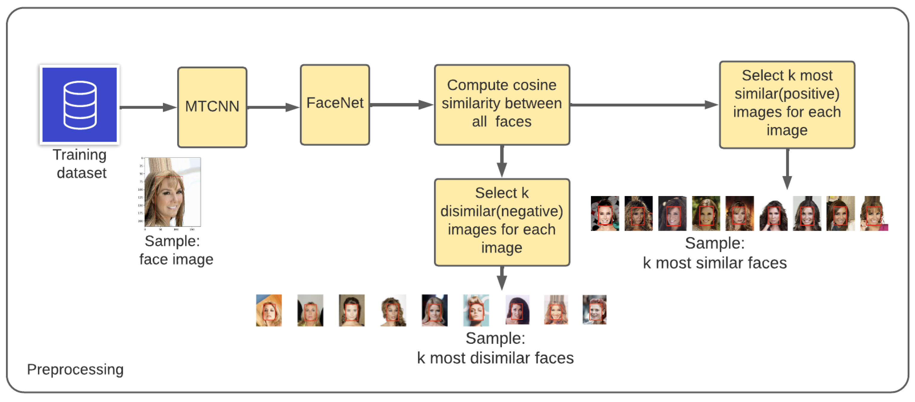
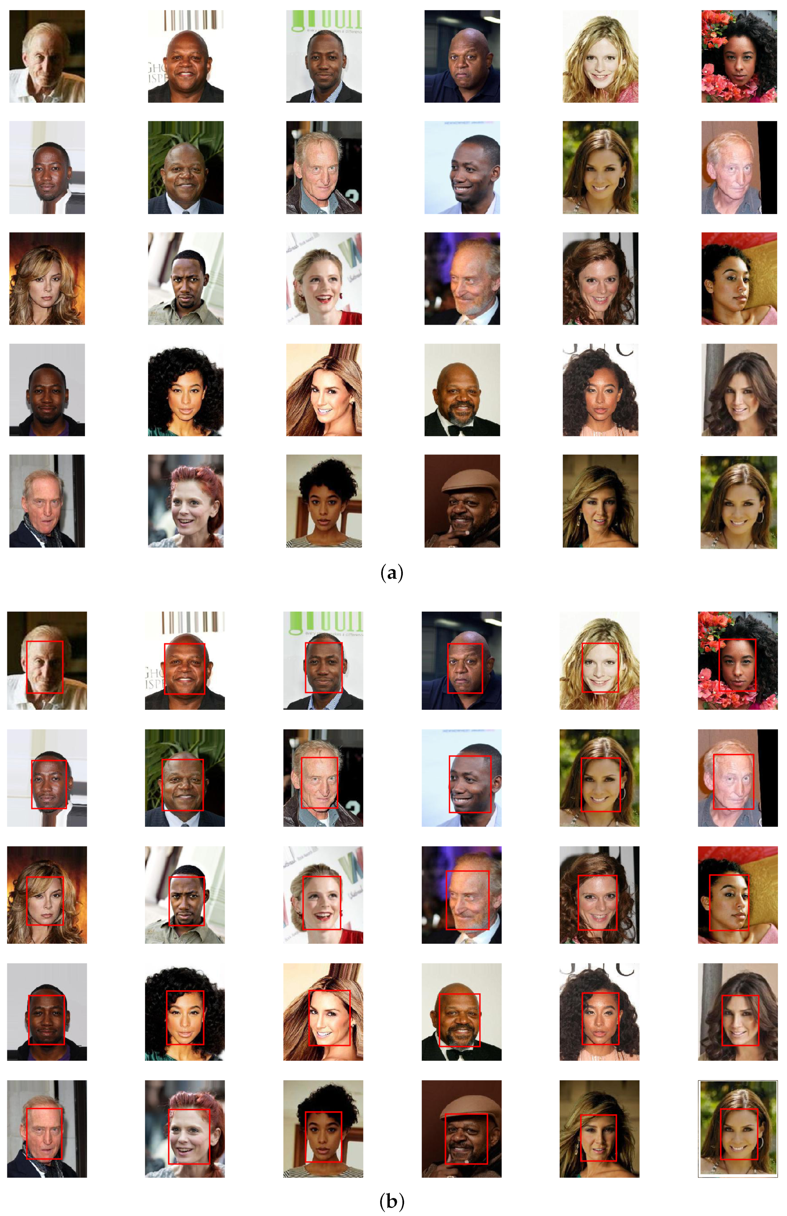
UFace first performs two preprocessing tasks, as shown in Figure 1. The first processing step is to detect a face from a given image using Multi-Task Cascaded Convolutional Neural Network (MTCNN) [46], which locates a face in a given image and draws a bounding box around it (see Figure 2b). It provides coordinates of the lower left corner of the bounding box plus its width and height, and resizes the image size to 112 by 112 pixels.

Secondly, it generates embedding vectors using the pre-trained Facenet model [8]. Then, we find the k most similar and k most dissimilar images for each image in the preprocessing phase. Note that Facenet is used here just to help calculate the cosine similarity/dissimilarity between images during the preprocessing stage, i.e., we did not use Facenet to train our models.

Algorithm 1 calculates the cosine similarity between a given image and all other remaining images in a dataset. Next, a threshold is used to select the k most similar and k most dissimilar images for each input image from the training dataset. To select the k most similar and k most dissimilar images, we experimented with different threshold values on validation set and empirically decided to use the optimal threshold (i.e., one that resulted in the highest accuracy). The optimal threshold value was found to be 0.6 for the most similar images and 0.2 for the most dissimilar images. In this way, we make sure any of the similar images are not the same as the dissimilar images.

Note that the value of k varies from image to image since a face can have a different number of most similar images. On average, however, we discovered that there are about 11 similar and dissimilar images for each image. In total, we created about 4 M training pairs (both for the similar and dissimilar pairs) for all images in the CelebA dataset (which has only about 200k images). The selection of the threshold value that is used to select the similar and dissimilar images is described in detail in the experimental section.

Algorithm 1 To select the k most similar and k most dissimilar images for each image in a dataset.

Require: The thresholds ths and thd, and m training images x Ensure: k most similar (${\tilde{x}}_{is}$) and k most dissimilar images (${\tilde{x}}_{id}$) for each image in a dataset, 1 ≤ i ≤ m, 1 ≤ p ≤ k and 1 ≤ n ≤ k     for $i\leftarrow 1$ to N, N←$length\left(m\right)$ do           for $j\leftarrow 1$ to N, N←$length\left(m\right)$ do                     if $i\ne j$                             ${\tilde{x}}_{ij}$ = cosine($x_i$, $x_j$)           end for     end for             Select k most similar images above the ths = 0.6, ${\tilde{x}}_{is}$ and randomly select k most dissimilar images below the thd = 0.2, ${\tilde{x}}_{id}$     end

Note that we used the Facenet pre-trained model only to calculate the cosine similarity between images during the pre-processing phase. However, the UFace training methods do not require to use Facenet and do not require explicitly labeled training data, as described in the training section.

2.2. Training

Note that the preprocessing and evaluation modules for both the autoencoder and Siamese networks are the same.

The state-of-the-art methods such as ArcFace [16], Facenet [8], GroupFace [19], CosFace [12], MegaFace [31], DeepFace [9], VGG Face [10] and Marginal Loss [15] require a very large amount of labeled data, which are difficult to obtain in many applications other than face images. For example, Facenet used about 200 M training images.

To address this problem, we propose an unsupervised deep learning face verification system using k most similar and k most dissimilar images, called UFace. To demonstrate the performance of UFace, we started using only k most similar images and the autoencoder network for verification. Next, we used both the k most similar and the k most dissimilar images with autoencoder. Since the latter gave better results than just using k most similar images, in the Siamese network we used both k most similar and k most dissimilar images.

2.2.1. UFace with Autoencoder Training

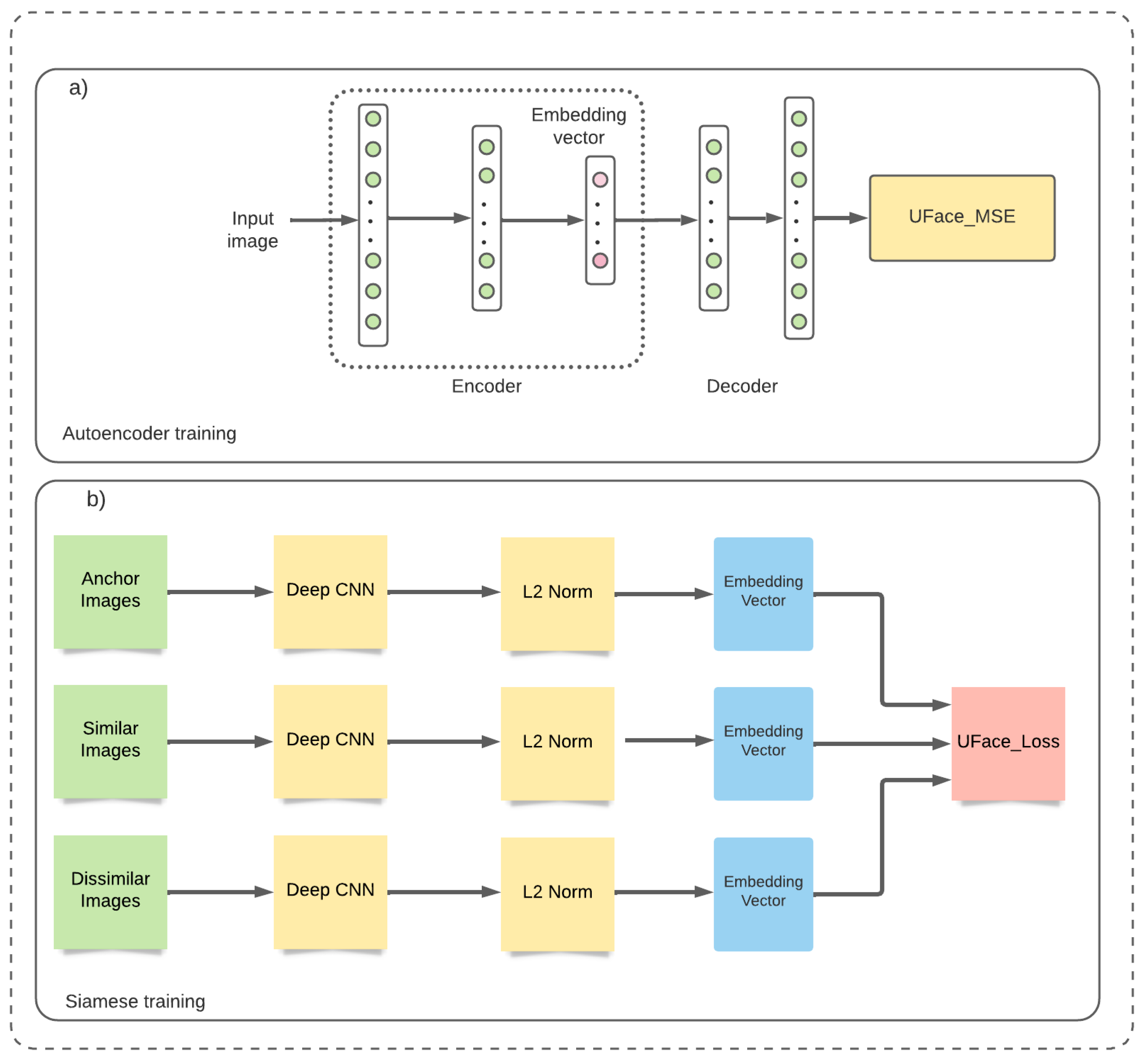
Classical Autoencoder Training: An autoencoder is an unsupervised neural network used in situations when no labeled data are available [47]. It is a feedforward neural network where the output (the compressed version of the input) is trained to be almost the same as the input. Autoencoders were successfully used in feature extraction [48], dimensionality reduction [49], image denoising [50] and image inpainting [51]. Autoencoder compresses high-dimensional input data, such as an image, into a lower-dimensional (compressed) representation and is trained to recreate the original input from its output. The difference between the reconstructed and the input image is the reconstruction error. The network is trained to minimize this error to find the best lower-dimensional representation, called the embedded vector. The autoencoder (AE) consists of (see Figure 3a) an encoder and decoder.

Encoder: The encoder part of the network maps the original input image into its lower-dimensional representation h.

$$h=g\left(\right(w\ast x)+b)$$

(1)

where w is a weight matrix between the input x and hidden layers, b is the bias and g is a nonlinear activation function.

Decoder: The decoder reconstructs the original input data from its encoded representation. In the decoding process, the AE maps h back to the original input approximation $\widehat{x}$.

$$\widehat{x}=f((\widehat{w}\ast h)+\widehat{b})$$

(2)

where ŵ is a weight matrix between the output of the encoder and hidden layers, $\widehat{x}$ is the output data, $\widehat{b}$ is bias and f is a nonlinear activation function.

The Mean Square Error (MSE) measures the reconstruction error [52,53]. The classical training is carried out by minimizing the average squared difference between the output value and the input value, as shown in Equation (3):

$${\displaystyle MeanSquaredError\left(MSE\right)=\frac{1}{m}\sum _{t=1}^m{(\widehat{x}-x)}^2}$$

(3)

where x is the original input and $\widehat{x}$ is the predicated value.

To make a fair comparison of the classical AE system with UFace, we developed our own classical AE system. Both systems are developed exactly in the same way except how the reconstruction error is computed. The classical AE system computes the reconstruction error with one original input image, whereas UFace computes the reconstruction error with k most similar and k most dissimilar images.

UFace Autoencoder Training: The UFace method is first demonstrated using only similar images. It trains the autoencoder to reconstruct k most similar images of the input image. Then, UFace is demonstrated using both similar and dissimilar images. It trains the autoencoder to reconstruct the k most similar and k most dissimilar images of the input image rather than the single input image, as is the case with classical autoencoder training. UFace uses the k most similar and k most dissimilar images of the input image during calculation of the reconstruction error, which is backpropagated to update the network weights.

State-of-the-art methods such as Facenet [8], Fusion [18], DeepFace [9], VGG Face [10] and Marginal Loss [15] require a very large amount of labeled data, which may be hard to obtain in many applications other than face images. For example, Facenet used about 200 M labeled training images.

To address this problem, we propose a novel training method that does not explicitly require a labeled training dataset. It trains the autoencoder to reconstruct the k most similar images of the input image rather than the single input image, as is the case with the classical autoencoder training. The new method uses the k most similar and k most dissimilar images of the input image during the calculation of the reconstruction error, which is backpropagated to update the network weights.

The autoencoder is trained by minimizing the loss function between the reconstructed image $\widehat{x}$ and the k most similar and k most dissimilar images of the original input image x for all images in the dataset.

The used training mechanism takes into account intra-person and inter-person face variabilities (k number of times), while in the classical autoencoder training mechanism, the loss function is computed only once. The value of k varies from image to image. In the first iteration, as shown in Equation (4), once the first input image is reconstructed it calculates the mean square error between the reconstructed image and the first kth most similar/dissimilar images (for the case of dissimilar images, it takes the negative value of the MSE). After calculating the error, it backpropagates the error to update the network parameters. In the second iteration, it continues training the same first input image and computes the mean square error with the second kth most similar/dissimilar images, and it continues training in the same way using the remaining kth most similar/dissimilar images. Once training for the first input image is completed, it starts training for the second input image in the same way, and continues for all images in the dataset. UFace calculation of the error is shown in Equation (4). The total number of training images is calculated as the sum of f(j), where f(j) is the function that outputs the total number of k most similar and k most dissimilar images in the training dataset. Since UFace computes the reconstruction errors 2k (k for the similar and k for the dissimilar images) times for each input face image, it accounts for face variabilities.

$${\displaystyle UFace\_MSE=\frac{1}{{\sum }_{i=1}^{m}f\left(j\right)}\sum _{i=1}^m\sum _{j=1}^{f\left(j\right)}{({\widehat{x}}_i-{\tilde{x}}_j)}^2}$$

(4)

UFace_MSE is the UFace loss function, where m is the number of training images, f(j) is the function that represents the variable number of k most similar images for the input image x${}_i$, $\widetilde{x_j}$ is most similar images for input image x${}_i$ and $\widehat{x_i}$ is the reconstructed image for the input image x${}_i$. Note that, for the case of dissimilar images, we take the negative of it since it will be maximized.

2.2.2. UFace with Siamese Training

The UFace training method on Siamese network using both similar and dissimilar images is shown in Figure 3b. It has three branches, each of which is the CNN encoder followed by the L2-normalization layer. The branches share the same weights. Branches for training are fed by an anchor (input image), similar images and dissimilar images. The output of the CNN encoder is known as image embedding. After the L2-normalization layer, the UFace loss function—UFace_Loss (Equation (5))—is computed as the error between the embeddings of similar and dissimilar images and the anchor. The loss function reduces deviation between the anchor and similar faces and increases deviation between the anchor and dissimilar faces. While training a model to classify, it optimizes the weights to minimize the loss function, i.e., to reduce the difference between similar faces and increase the difference between dissimilar faces. During the training phase, every input consists of 3 images of faces. Two images are of the same person (one image is considered as anchor and the second is a similar image), and the third is of a different person (dissimilar).

The UFace_Loss (using both k similar and k dissimilar images) loss is computed as

$${\displaystyle \sum _{i=1}^N\sum _{j=1}^{f\left(j\right)}(d(f\left(x_i^a\right)-f\left(x_j^p\right))-d(f\left(x_i^a\right)-f\left(x_j^n\right)))+\alpha }$$

(5)

where f(x) takes x as an input and returns an embedding vector, i denotes the ith input, j denotes the jth similar and dissimilar images for the ith input image, a is an anchor image, p is a similar image, n is a dissimilar image, N is the number of training data and f(j) is the function that represents the variable number of k most similar and k most dissimilar images for the input image $x_i$. The $\alpha$ is a margin that is enforced between positive and negative pairs. It ensure that the model does not make the embeddings equal each other to trivially satisfy the above inequality.

Minimizing the above equation means minimizing the first term (distance between anchor and similar image) and maximizing the second term (distance between anchor and dissimilar image).

As shown in Figure 3b, in UFace Siamese training, the network uses three branches: the anchor, k most similar faces of the anchor and k most dissimilar faces of the anchor. First, the three branches are fed into the CNN network using 112 by 112 pixel images. The CNN encodes the pixel values and provides face embedding vector. Then, the loss between the embedding of the anchor and similar and dissimilar faces is computed. By Equation (5), for each anchor image, the loss function is computed 2 times k, where k is the most similar and k dissimilar images with the anchor.

2.3. Evaluation

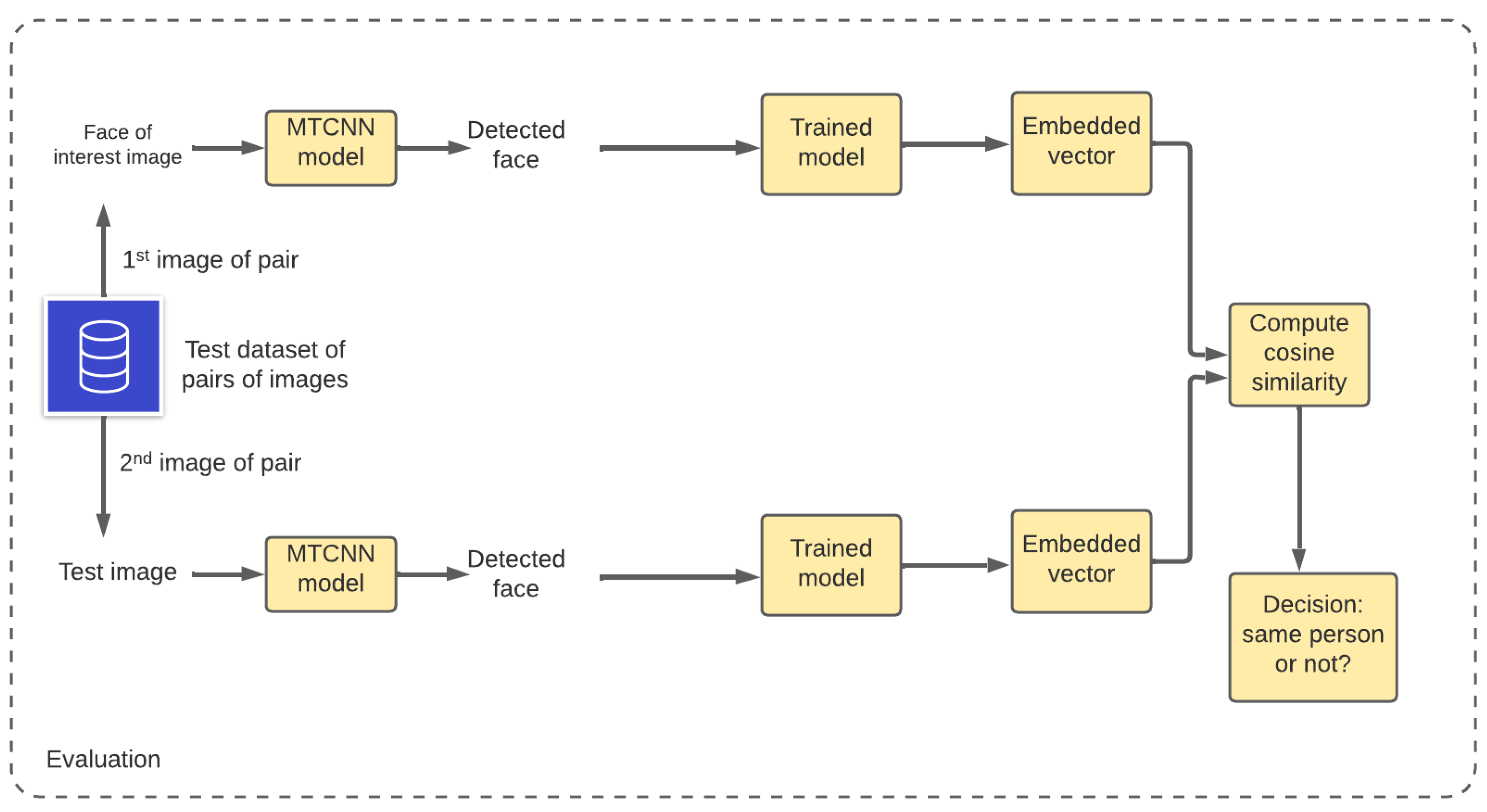
As shown in Figure 4, the goal of face image verification is to decide if two face images belong to the same person or not. Given a pair of input face images, we first use MTCNN to detect faces from the given images. Then, image embeddings are extracted using any encoder branch of the network for the pairs of test images. Cosine similarity is computed between the two embedding vectors. If the cosine similarity is above the given threshold value, the two images belong to the same person, and not otherwise.

3. Datasets Used

CelebA [54] is a dataset that has over 200 K images of 10,177 celebrities, which include pose variations and background clutter; it was used for training UFace.

The Labeled Faces in the Wild dataset (LFW) [29] contains 13,233 images of 5749 people. For testing, the database is randomly (uniformly) split into 10 subsets. Next, 300 matched (of the same person) pairs and 300 mismatched (of different persons) pairs are randomly chosen within each subset. In other words, for testing, 3000 (10 × 300) matched and 3000 mismatched pairs [29] were used.

The YouTube Faces dataset (YTF) [30] of face videos contains 3425 videos of 1595 people collected from YouTube, with an average of two videos per person. The shortest clip duration is 48 frames and the longest is 6070 frames. The average length of a video clip is 181 frames. For testing, 5 K video pairs are randomly chosen and prepared, half of which are pairs of videos of the same person and half are of different people. Thus, for testing, 5 K pairs of static images with 2500 of them of the same person and 2500 not of the same person [30] were used.

Cross-age LFW (CALFW) [55] is a newer version of LFW in which 3000 similar face pairs at different ages and 3000 dissimilar face pairs of the same gender are present to reduce the influence of attribute differences between similar/dissimilar pairs. Thus, for testing, 6 K pairs of face images were used.

Celebrities in FrontalProfile in the Wild (CFP-FP) [56] is another face verification benchmark dataset with 7000 face images, of which 3500 are same person pairs and 3500 are different person pairs. Thus, for testing, 7 K pairs of face images were used.

4. Experiments

UFace was trained on the CelebA dataset and its performance was tested on four benchmark datasets: LFW, YTF, CALFW and CFP-FP.

4.1. Experimental Setup

The Keras deep learning library [57] was used to train the model. It is trained for 100 epochs or until the error is not decreasing, using a batch size of 100 images. It uses backpropagation with stochastic gradient descent (SGD), momentum of 0.91, weight decay of 0.00001 and a logarithmically decaying learning rate from ${10}^{-2}$ to ${10}^{-8}$. The dimension of the input images is 112 by 112 pixels.

In order to select the best threshold value, which is used to select the number of similar and dissimilar images for each image, we selected about 10% of the images from the training set and selected the similar and dissimilar images using different threshold values (i.e., from 0.1 to 0.7). We used about 10% of the images as a validation set to tune the threshold value. Thus, all cosine distance scores less than the threshold values were considered as dissimilar images and all cosine distance scores greater than the threshold values were considered as similar images. For example, if we take the threshold values of 0.6 and 0.2, all cosine distances less than 0.2 are considered as dissimilar and all cosine distance scores above 0.6 are considered as similar images.

The reason for selecting two different threshold values is to choose similar and dissimilar images correctly. The threshold values were optimized experimentally by changing their values from 0.1 to 0.9 and choosing the ones that resulted in the highest accuracy on the validation dataset; the threshold 0.6 was chosen for the similar images and threshold 0.2 for the dissimilar images (to a given image).

After computing the most similar and dissimilar images for each threshold value, we have trained different models (i.e., one model for each threshold value). After training the model, we computed the accuracy of each model on other 1 K datasets that were selected from the validation set.

Using threshold values of 0.6 and 0.2 gives us the highest accuracy. Thus, we selected 0.6 and 0.2 as threshold values for similar and dissimilar images, respectively, and selected the most similar/dissimilar images on the remaining 180 K training images. Note that we used two threshold values, one to select the similar images and the other to select the dissimilar images; thus, we can reduce the possibility of dissimilar images being selected as similar images and vice versa. A total 10% of the training dataset was used for validation in order to select the best threshold values.

The training was performed using the CelebA [54] dataset. First, the face is detected, including the bounding box around the face. Then, the cosine similarity for each face against the remaining faces in the training dataset is computed. Then, the threshold values are chosen experimentally to select the k most similar and k most dissimilar images for each image.

The autoencoder is a fully connected feed-forward network consisting of 3 hidden layers. As shown in Figure 3a, the encoder and decoder are symmetrical. The encoder input and decoder output each have 112 by 112 neurons. The second layer in both the encoder and decoder has 800 neurons. The output of the encoder has 300 neurons, which determines the size of the embedding vector.

The Siamese network has 3 branches, each of which is the CNN encoder followed by the L2-normalization layer. The CNN encoder block is a Resnet100 architecture [47]. It consists of five main layers where each layer contains convolutional and identity blocks. The first layer contains max-pooling and the last layer contains average pooling. The five layers are followed by two fully connected layers of 800 and 300 neurons, respectively. The CNN encoder encodes the input images (112 by 112) into a 300-dimensional image embedding vector. Note that in addition to convolutional, identity and max-pooling layers, it also uses batch normalization [58] and dropout [59].

4.2. UFace Training Using Autoencoder and Comparing It with Classical Autoencoder Training

As it is shown in

Table 1. Accuracy using classical autoencoder *, modified autoencoder with k most similar images ** and modified autoencoder with both k most similar and k most dissimilar images ***.

Model	LFW	YTF	CALFW	CFP-FP
UFace *	92.76	89.97	89.22	91.88
UFace **	95.81	93.24	92.63	95.13
UFace ***	96.42	93.92	93.08	95.78

, UFace using autoencoder provides better results than the one based on classical autoencoder training. Note that we use classical autoencoder training as the baseline system. Table 1 shows that the baseline accuracies are 92.76%, 89.97%, 89.22% and 91.88% on LFW, YTF, CALFW and CFP-FP datasets, respectively. It is compared with two UFace models: UFace autoencoder training method using only the k most similar images and UFace autoencoder training using both the k most similar and k most dissimilar images.

From Table 1, we see that UFace using autoencoder that uses only the k most similar images results in 95.81%, 93.24%, 92.63% and 95.13% accuracies on the LFW, TYF, CALFW and CFP-FP datasets, respectively. The improvements over the classical autoencoder represent a 3.05%, 3.24%, 3.41% and 3.25% improvement on the LFW, YTF, CALFW and CFP-FP datasets, respectively.

Next, we assess the impact of using also the k most dissimilar images. Table 1 shows that using both the k most similar and k most dissimilar images results in 96.42%, 93.92%, 93.08% and 95.78% accuracies on the LFW, YTF, CALFW and CFP-FP datasets, respectively. Thus, using dissimilar images, in addition to the similar images, results in a slight improvement over using only the similar images (i.e., 96.42% vs. 95.81% on LFW, 93.92% vs. 93.24% on YTF, 93.08% vs. 92.63% on CALFW and 95.78% vs. 95.13% on CFP-FP). If we compare the UFace autoencoder method that uses both the similar and dissimilar images with the classical autoencoder training method, it provides us 3.66%, 3.95%, 3.86% and 3.9% improvement on LFW, YTF, CALFW and CFP-FP datasets, respectively. Thus, the results reported in Table 1 show the advantage of UFace demonstrated on an autoencoder network that uses both the k most similar and k most dissimilar images.

4.3. UFace Training Using Siamese Network

In addition to demonstrating UFace training using the autoencoder network, we also demonstrated UFace training using the Siamese network and compared the performance of the UFace with different state-of-art face verification systems.

4.3.1. Comparison of UFace on LFW Dataset

Table 2. Comparison of UFace results using Siamese network with both k most similar and k most dissimilar face images with those of some state-of-the-art methods on the LFW testing dataset.

Model	Training Data Size	Labeled/Unlabeled	Testing Data Size	Testing Accuracy (%)
Fusion	500 M	Labeled	6 K	98.37 [18]
Facenet	200 M	Labeled	6 K	99.63 [8]
UniformFace	6.1 M	Labeled	6 K	99.80 [60]
ArcFace	5.8 M	Labeled	6 K	99.82 [16]
GroupFace	5.8 M	Labeled	6 K	99.85 [19]
CosFace	5 M	Labeled	6 K	99.73 [12]
DeepFace-ensemble	4.4 M	Labeled	6 K	97.35 [9]
Marginal Loss	4 M	Labeled	6 K	99.48 [15]
CurricularFace	3.8 M	Labeled	6 K	99.80 [13]
RegularFace	3.1 M	Labeled	6 K	99.61 [61]
AFRN	3.1 M	Labeled	6 K	99.85 [62]
VGG Face	2.6 M	Labeled	6 K	98.95 [10]
Stream Loss	1.5 M	Labeled	6 K	98.97 [63]
MDCNN	1 M	Labeled	6 K	99.38 [32]
PSO AlexNet TL	14 M	Labeled	6 K	99.57 [33]
ULNet	1 M	Labeled	6 K	99.70 [64]
Ben Face	0.5 M	Labeled	6 K	99.20 [34]
F${}^2$C	5.8 M	Labeled	6 K	99.83 [65]
PCCycleGAN	0.5 M	Unlabeled	6 K	99.52 [43]
CAPG GAN	1 M	Unlabeled	6 K	99.37 [44]
UFace	200 K	Unlabeled	6 K	99.40

shows a comparison of UFace with the state-of-the-art methods. Note that we compare our best result with the state-of-the-art systems that use both supervised and unsupervised training, whereas the UFace training does not explicitly required labeled data.

Although most of the methods such as ArcFace, GroupFace, Marginal Loss and CosFace have slightly better accuracy than UFace, UFace is trained on a much smaller dataset (about 200 K images) while most of the state-of-the-art methods use millions of training images.

UFace with Siamese network achieves an accuracy of 99.40%, which is on par both with the state-of-the-art supervised and unsupervised systems. For example, the ArcFace used 5.8 M labeled images to achieve 99.82% accuracy, whereas UFace accuracy is 99.40% but required only about 200 K images for training.

4.3.2. Comparison of the UFace on YTF Dataset

Similarly, we compare the UFace with Siamese network using similar and dissimilar images with state-of-the-art supervised and unsupervised systems on the YTF dataset. In

Table 3. Comparison of UFace results using Siamese network with both k most similar and k most dissimilar face images with those of some state-of-the-art methods on the YTF testing dataset.

Model	Training Data Size	Labeled/Unlabeled	Testing Data Size	Testing Accuracy (%)
Facenet	200 M	Labeled	5 K	95.12 [8]
UniformFace	6.1 M	Labeled	5 K	97.70 [60]
ArcFace	5.8 M	Labeled	5 K	98.02 [16]
GroupFace	5.8 M	Labeled	5 K	97.80 [19]
CosFace	5 M	Labeled	5 K	97.60 [12]
DeepFace-single	4.4 M	Labeled	5 K	91.40 [9]
Marginal Loss	4 M	Labeled	5 K	95.98 [15]
RegularFace	3.1 M	Labeled	5 K	96.70 [61]
AFRN	3.1 M	Labeled	5 K	97.70 [62]
NAN	3 M	Labeled	5 K	95.70 [66]
VGG Face	2.6 M	Labeled	5 K	97.30 [10]
Stream Loss	1.5 M	Labeled	5 K	96.40 [63]
MDCNN	1 M	Labeled	5 K	94.69 [32]
Ben Face	0.5 M	Labeled	5 K	96.63 [34]
F${}^2$C	1 M	Labeled	5 K	97.76 [65]
CORAL	0.5 M	Unlabeled	5 K	94.50 [45]
UDAFRUV	0.5 M	Unlabeled	5 K	95.38 [67]
UFace	200 K	Unlabeled	5 K	96.04

, VGG Face [10] used 2.6 M labeled training data and achieved slightly over 97% accuracy. In [15], the authors used marginal loss and a labeled 4 M training dataset to achieve a comparable result with Facenet [8], which used 200 M labeled training data and achieved over 95% accuracy. The drawback of these methods, however, is that they require a huge labeled dataset for training. On the other hand, UFace uses much less and unlabeled training data to achieve over 96% accuracy. Although, if we compare the UFace Siamese with both the state-of-the-art supervised and unsupervised systems on YTF, its accuracy (i.e., 96.04%) is slightly better than some of the supervised systems, better than the unsupervised systems and almost close to state-of-the-art methods such as ArcFace, GroupFace, CostFace and VGG Face.

4.3.3. Comparison of UFace on CALFW and CFP-FP Datasets

In addition to LFW and YTF, the results of UFace have been compared against both state-of-the-art supervised and unsupervised systems on the CALFW and CFP-FP datasets.

Table 4. Comparison of UFace results using Siamese network with both k most similar and k most dissimilar face images with those of some state-of-the-art methods on the CALFW testing dataset.

Model	Training Data Size	Labeled or Unlabeled	Testing Data Size	Testing Accuracy (%)
ArcFace	5.8 M	Labeled	6 K	95.45 [16]
GroupFace	5.8 M	Labeled	6 K	96.20 [19]
CurricularFace	3.8 M	labeled	6 K	96.20 [13]
MegaFace	3.8 M	Labeled	6 K	96.15 [31]
ULNet	1 M	Labeled	6 K	95.71 [64]
F${}^2$C	1 M	Labeled	6 K	95.25 [65]
UFace	200 K	Unlabeled	6 K	95.12

and

Table 5. Comparison of UFace results using Siamese network with both k most similar and k most dissimilar face images with those of some state-of-the-art methods on the CFP-FP testing dataset.

Model	Training Data Size	Labeled or Unlabeled	Testing Data Size	Testing Accuracy (%)
ArcFace	5.8 M	Labeled	7 K	98.27 [16]
GroupFace	5.8 M	Labeled	7 K	98.63 [19]
CurricularFace	3.8 M	Labeled	7 K	98.37 [13]
Dyn-ArcFace	5.8 M	Labeled	7 K	94.25 [68]
MegaFace	3.8 M	Labeled	7 K	98.46 [31]
CircleLoss	5.8 M	Labeled	7 K	96.02 [69]
ULNet	1 M	Labeled	7 K	98.23 [64]
F${}^2$C	1 M	Labeled	7 K	98.25 [65]
IMAN	0.5 M	Unlabeled	7 K	92.74 [70]
UFace	200 K	Unlabeled	7 K	97.89

show that UFace’s results are close to those of ArcFace. However, the results of the UFace are a bit lower than the GroupFace, CurriculaFace and MegaFace models. If we compare our best results with both supervised and unsupervised ones, Table 5 shows that our results are on par with the state-of-the-art unsupervised systems.

The UFace has the following advantages over the state-of-the-art systems. Firstly, while the UFace does not explicitly require labeled training data, the state-of-the-art methods do. Secondly, the UFace requires only about 200 K training data, whereas the state-of-the-art use a minimum of 3.8 M and maximum of 5.8 M. Thirdly, the training time of UFace is much less than that of the state-of-the-art ones because of the amount of training data. Lastly, the results of UFace are comparable to the state-of-the-art.

5. Conclusions

The state-of-the art deep learning methods for face verification usually require large amounts of labeled data for training. However, it is not always easy to obtain such data. To address this problem, we proposed a novel unsupervised deep learning face verification system (UFace) that uses k most similar and k most dissimilar images to a given image that are selected from unlabeled data.

UFace’s performance was evaluated using both the autoencoder approach and Siamese networks approach. As Siamese networks performed much better than the autoencoder, they were used for all the presented comparisons with state-of-the-art algorithms. Unlike in the classical neural network training, UFace computes its loss function k times with the similar images and k times with the dissimilar images (for a total of 2xk times) for each input image. UFace is evaluated on four benchmark face verification datasets, namely, Labeled Faces in the Wild (LFW), YouTube Faces (YTF), Cross-age LFW (CALFW) and Celebrities in Frontal Profile in the Wild (CFP-FP). Its performance using the Siamese network achieved accuracies of 99.40%, 96.04%, 95.12% and 97.89%, respectively, which are comparable with the state-of-the-art methods even though UFace uses much less data for training.

Additional advantage of UFace is that it can be used for verification of other types of images in domains where labeled data are not available at all.

References

- Jain, A.; Li, S. Handbook of Face Recognition; Springer: Berlin/Heidelberg, Germany, 2011. [Google Scholar]
- Woubie, A.; Koivisto, L.; Bäckström, T. Voice-quality Features for Deep Neural Network Based Speaker Verification Systems. In Proceedings of the 2021 29th European Signal Processing Conference (EUSIPCO), Dublin, Ireland, 23–27 August 2021; pp. 176–180. [Google Scholar]
- Nagrani, A.; Chung, J.; Xie, W.; Zisserman, A. Voxceleb: Large-scale speaker verification in the wild. Comput. Speech Lang. 2020, 60, 101027. [Google Scholar] [CrossRef]
- He, K.; Zhang, X.; Ren, S.; Sun, J. Deep residual learning for image recognition. In Proceedings of the IEEE Conference On Computer Vision And Pattern Recognition, Las Vegas, NV, USA, 27–30 June 2016; pp. 770–778. [Google Scholar]
- Cios, K.; Shin, I. Image recognition neural network: IRNN. Neurocomputing 1995, 7, 159–185. [Google Scholar] [CrossRef]
- Shin, J.; Smith, D.; Swiercz, W.; Staley, K.; Rickard, J.; Montero, J.; Kurgan, L.; Cios, K. Recognition of partially occluded and rotated images with a network of spiking neurons. IEEE Trans. Neural Netw. 2010, 21, 1697–1709. [Google Scholar] [CrossRef] [PubMed]
- Cachi, P.; Ventura, S.; Cios, K. CRBA: A Competitive Rate-Based Algorithm Based on Competitive Spiking Neural Networks. Front. Comput. Neurosci. 2021, 15, 627567. [Google Scholar] [CrossRef] [PubMed]
- Schroff, F.; Kalenichenko, D.; Philbin, J. Facenet: A unified embedding for face recognition and clustering. In Proceedings of the IEEE Conference on Computer Vision and Pattern Recognition, Boston, MA, USA, 7–12 June 2015; pp. 815–823. [Google Scholar]
- Taigman, Y.; Yang, M.; Ranzato, M.; Wolf, L. Deepface: Closing the gap to human-level performance in face verification. In Proceedings of the IEEE Conference On Computer Vision And Pattern Recognition, Columbus, OH, USA, 23–28 June 2014; pp. 1701–1708. [Google Scholar]
- Parkhi, O.; Vedaldi, A.; Zisserman, A. Deep Face Recognition. British Machine Vision Association. 2015. Available online: http://www.bmva.org/bmvc/2015/papers/paper041/paper041.pdf (accessed on 11 May 2022).
- Zhu, Z.; Luo, P.; Wang, X.; Tang, X. Recover canonical-view faces in the wild with deep neural networks. arXiv 2014, arXiv:1404.3543. [Google Scholar]
- Wang, H.; Wang, Y.; Zhou, Z.; Ji, X.; Gong, D.; Zhou, J.; Li, Z.; Liu, W. Cosface: Large margin cosine loss for deep face recognition. In Proceedings of the IEEE Conference on Computer Vision and Pattern Recognition, Salt Lake City, UT, USA, 18–23 June 2018; pp. 5265–5274. [Google Scholar]
- Huang, Y.; Wang, Y.; Tai, Y.; Liu, X.; Shen, P.; Li, S.; Li, J.; Huang, F. Curricularface: Adaptive curriculum learning loss for deep face recognition. In Proceedings of the IEEE/CVF Conference on Computer Vision and Pattern Recognition, Seattle, WA, USA, 13–19 June 2020; pp. 5901–5910. [Google Scholar]
- Deng, J.; Guo, J.; Yang, J.; Lattas, A.; Zafeiriou, S. Variational prototype learning for deep face recognition. In Proceedings of the IEEE/CVF Conference on Computer Vision and Pattern Recognition, Nashville, TN, USA, 20–25 June 2021; pp. 11906–11915. [Google Scholar]
- Deng, J.; Zhou, Y.; Zafeiriou, S. Marginal loss for deep face recognition. In Proceedings of the IEEE Conference on Computer Vision and Pattern Recognition Workshops, Honolulu, HI, USA, 21–26 July 2017; pp. 60–68. [Google Scholar]
- Deng, J.; Guo, J.; Xue, N.; Zafeiriou, S. Arcface: Additive angular margin loss for deep face recognition. In Proceedings of the IEEE/CVF Conference on Computer Vision and Pattern Recognition, Long Beach, CA, USA, 15–20 June 2019; pp. 4690–4699. [Google Scholar]
- Sun, Y.; Liang, D.; Wang, X.; Tang, X. Deepid3: Face recognition with very deep neural networks. arXiv 2015, arXiv:1502.00873. [Google Scholar]
- Taigman, Y.; Yang, M.; Ranzato, M.; Wolf, L. Web-scale training for face identification. In Proceedings of the IEEE Conference on Computer Vision and Pattern Recognition, Boston, MA, USA, 7–12 June 2015; pp. 2746–2754. [Google Scholar]
- Kim, Y.; Park, W.; Roh, M.; Shin, J. Groupface: Learning latent groups and constructing group-based representations for face recognition. In Proceedings of the IEEE/CVF Conference on Computer Vision and Pattern Recognition, Seattle, WA, USA, 13–19 June 2020; pp. 5621–5630. [Google Scholar]
- Wang, X.; Zhang, S.; Wang, S.; Fu, T.; Shi, H.; Mei, T. Mis-classified vector guided softmax loss for face recognition. AAAI Conf. Artif. Intell. 2020, 34, 12241–12248. [Google Scholar] [CrossRef]
- Zhang, J.; Yan, X.; Cheng, Z.; Shen, X. A face recognition algorithm based on feature fusion. Concurr. Comput. Pract. Exp. 2022, 34, e5748. [Google Scholar] [CrossRef]
- Marcialis, G.; Roli, F. Fusion of LDA and PCA for Face Verification. In Proceedings of the International Workshop on Biometric Authentication, Copenhagen, Denmark, 1 June 2002; pp. 30–37. [Google Scholar]
- Marcel, S.; Bengio, S. Improving face verification using skin color information. Object Recognit. Support. User Interact. Serv. Robot. 2022, 2, 378–381. [Google Scholar]
- McCool, C.; Marcel, S. Parts-based face verification using local frequency bands. In Proceedings of the International Conference on Biometrics, Alghero, Italy, 2–5 June 2009; pp. 259–268. [Google Scholar]
- Pereira, T.; Angeloni, M.; Simões, F.; Silva, J. Video-based face verification with local binary patterns and svm using gmm supervectors. In Proceedings of the International Conference on Computational Science and Its Applications, Salvador de Bahia, Brazil, 8–21 June 2012; pp. 240–252. [Google Scholar]
- Wang, Y.; Wu, Q. Research on Face Recognition Technology Based on PCA and SVM. In Proceedings of the 2022 7th International Conference on Big Data Analytics (ICBDA), Guangzhou, China, 4–6 March 2022; pp. 248–252. [Google Scholar]
- Serson, C.; Saban, M.; Gao, Y. On local features for GMM based face verification. In Proceedings of the Third International Conference on Information Technology and Applications (ICITA’05), Sydney, Australia, 4–7 July 2005; Volume 1, pp. 650–655. [Google Scholar]
- Bromley, J.; Guyon, I.; LeCun, Y.; Säckinger, E.; Shah, R. Signature verification using a" siamese" time delay neural network. Adv. Neural Inf. Process. Syst. 1993, 6, 737–744. [Google Scholar] [CrossRef] [Green Version]
- Huang, G.; Mattar, M.; Berg, T.; Learned-Miller, E. Labeled Faces in the Wild: A Database Forstudying Face Recognition in Unconstrained Environments. 2008. Available online: https://hal.inria.fr/inria-00321923 (accessed on 10 May 2022).
- Wolf, L.; Hassner, T.; Maoz, I. Face recognition in unconstrained videos with matched background similarity. In Proceedings of the CVPR, Colorado Springs, CO, USA, 20–25 June 2011; pp. 529–534. [Google Scholar]
- Meng, Q.; Zhao, S.; Huang, Z.; Zhou, F. Magface: A universal representation for face recognition and quality assessment. In Proceedings of the IEEE/CVF Conference on Computer Vision and Pattern Recognition, Nashville, TN, USA, 20–25 June 2021; pp. 14225–14234. [Google Scholar]
- Huang, X.; Zeng, X.; Wu, Q.; Lu, Y.; Huang, X.; Zheng, H. Face Verification Based on Deep Learning for Person Tracking in Hazardous Goods Factories. Processes 2022, 10, 380. [Google Scholar] [CrossRef]
- Elaggoune, H.; Belahcene, M.; Bourennane, S. Hybrid descriptor and optimized CNN with transfer learning for face recognition. Multimed. Tools Appl. 2022, 81, 9403–9427. [Google Scholar] [CrossRef]
- Ben Fredj, H.; Bouguezzi, S.; Souani, C. Face recognition in unconstrained environment with CNN. Vis. Comput. 2021, 37, 217–226. [Google Scholar] [CrossRef]
- Xie, Q.; Dai, Z.; Hovy, E.; Luong, T.; Le, Q. Unsupervised data augmentation for consistency training. Adv. Neural Inf. Process. Syst. 2020, 33, 6256–6268. [Google Scholar]
- Sohn, K.; Berthelot, D.; Carlini, N.; Zhang, Z.; Zhang, H.; Raffel, C.; Cubuk, E.; Kurakin, A.; Li, C. Fixmatch: Simplifying semi-supervised learning with consistency and confidence. Adv. Neural Inf. Process. Syst. 2020, 33, 596–608. [Google Scholar]
- Caron, M.; Bojanowski, P.; Joulin, A.; Douze, M. Deep clustering for unsupervised learning of visual features. In Proceedings of the European Conference on Computer Vision (ECCV), Munich, Germany, 8–14 September 2018; pp. 132–149. [Google Scholar]
- Gidaris, S.; Singh, P.; Komodakis, N. Unsupervised representation learning by predicting image rotations. arXiv 2018, arXiv:1803.07728. [Google Scholar]
- Shu, Y.; Yan, Y.; Chen, S.; Xue, J.; Shen, C.; Wang, H. Learning spatial-semantic relationship for facial attribute recognition with limited labeled data. In Proceedings of the IEEE/CVF Conference on Computer Vision and Pattern Recognition, Nashville, TN, USA, 20–25 June 2021; pp. 11916–11925. [Google Scholar]
- He, M.; Zhang, J.; Shan, S.; Chen, X. Enhancing Face Recognition With Self-Supervised 3D Reconstruction. In Proceedings of the IEEE/CVF Conference on Computer Vision and Pattern Recognition, New Orleans, Louisiana, USA, 21–24 June 2022; pp. 4062–4071. [Google Scholar]
- Yin, J.; Xu, Y.; Wang, N.; Li, Y.; Guo, S. Mask Guided Unsupervised Face Frontalization using 3D Morphable Model from Single-View Images: A face frontalization framework that can generate identity preserving frontal view image while maintaining the background and color tone from input with only front images for training using 3D Morphable Model. In Proceedings of the 2022 4th Asia Pacific Information Technology Conference, Bangkok, Thailand, 14–16 January 2022; pp. 23–30. [Google Scholar]
- Khan, M.; Jabeen, S.; Khan, M.; Saba, T.; Rehmat, A.; Rehman, A.; Tariq, U. A realistic image generation of face from text description using the fully trained generative adversarial networks. IEEE Access 2020, 9, 1250–1260. [Google Scholar] [CrossRef]
- Liu, Y.; Chen, J. Unsupervised face frontalization for pose-invariant face recognition. Image Vis. Comput. 2021, 106, 104093. [Google Scholar] [CrossRef]
- Hu, Y.; Wu, X.; Yu, B.; He, R.; Sun, Z. Pose-guided photorealistic face rotation. In Proceedings of the IEEE Conference on Computer Vision and Pattern Recognition, Salt Lake City, UT, USA, 18–23 June 2018; pp. 8398–8406. [Google Scholar]
- Sun, B.; Feng, J.; Saenko, K. Return of frustratingly easy domain adaptation. In Proceedings of the AAAI Conference on Artificial Intelligence, Austin, TX, USA, 25–30 January 2015; Volume 30. [Google Scholar]
- Zhang, K.; Zhang, Z.; Li, Z.; Qiao, Y. Joint face detection and alignment using multitask cascaded convolutional networks. IEEE Signal Process. Lett. 2016, 23, 1499–1503. [Google Scholar] [CrossRef] [Green Version]
- Szegedy, C.; Ioffe, S.; Vanhoucke, V.; Alemi, A. Inception-v4, inception-resnet and the impact of residual connections on learning. In Proceedings of the AAAI Conference on Artificial Intelligence, San Francisco, CA, USA, 4–9 February 2017; Volume 31. [Google Scholar]
- Zabalza, J.; Ren, J.; Zheng, J.; Zhao, H.; Qing, C.; Yang, Z.; Du, P.; Marshall, S. Novel segmented stacked autoencoder for effective dimensionality reduction and feature extraction in hyperspectral imaging. Neurocomputing 2016, 185, 1–10. [Google Scholar] [CrossRef] [Green Version]
- Makhzani, A.; Shlens, J.; Jaitly, N.; Goodfellow, I.; Frey, B. Adversarial autoencoders. arXiv 2015, arXiv:1511.05644. [Google Scholar]
- Vincent, P.; Larochelle, H.; Lajoie, I.; Bengio, Y.; Manzagol, P.; Bottou, L. Stacked denoising autoencoders: Learning useful representations in a deep network with a local denoising criterion. J. Mach. Learn. Res. 2010, 11, 3371–3408. [Google Scholar]
- Pathak, D.; Krahenbuhl, P.; Donahue, J.; Darrell, T.; Efros, A. Context encoders: Feature learning by inpainting. In Proceedings of the IEEE Conference on Computer Vision and Pattern Recognition, Las Vegas, NV, USA, 27–30 June 2016; pp. 2536–2544. [Google Scholar]
- Ling, Z.; Kang, S.; Zen, H.; Senior, A.; Schuster, M.; Qian, X.; Meng, H.; Deng, L. Deep learning for acoustic modeling in parametric speech generation: A systematic review of existing techniques and future trends. IEEE Signal Process. Mag. 2015, 32, 35–52. [Google Scholar] [CrossRef]
- Liu, W.; Wang, Z.; Liu, X.; Zeng, N.; Liu, Y.; Alsaadi, F. A survey of deep neural network architectures and their applications. Neurocomputing 2017, 234, 11–26. [Google Scholar] [CrossRef]
- Liu, Z.; Luo, P.; Wang, X.; Tang, X. Deep learning face attributes in the wild. In Proceedings of the IEEE International Conference on Computer Vision, Santiago, Chile, 7–13 December 2015; pp. 3730–3738. [Google Scholar]
- Zheng, T.; Deng, W.; Hu, J. Cross-age lfw: A database for studying cross-age face recognition in unconstrained environments. arXiv 2017, arXiv:1708.08197. [Google Scholar]
- Sengupta, S.; Chen, J.C.; Castillo, C.; Patel, V.M.; Chellappa, R.; Jacobs, D.W. Frontal to Profile Face Verification in the Wild. In Proceedings of the IEEE Conference on Applications of Computer Vision, Lake Placid, NY, USA, 7–10 March 2016. [Google Scholar]
- Chollet, F. Keras, GitHub. 2015. Available online: https://github.com/fchollet/keras (accessed on 11 May 2022).
- Ioffe, S.; Szegedy, C. Batch normalization: Accelerating deep network training by reducing internal covariate shift. In Proceedings of the International Conference on Machine Learning, Lille, France, 6–11 July 2015; pp. 448–456. [Google Scholar]
- Srivastava, N.; Hinton, G.; Krizhevsky, A.; Sutskever, I.; Salakhutdinov, R. Dropout: A simple way to prevent neural networks from overfitting. J. Mach. Learn. Res. 2014, 15, 1929–1958. [Google Scholar]
- Duan, Y.; Lu, J.; Zhou, J. Uniformface: Learning deep equidistributed representation for face recognition. In Proceedings of the IEEE/CVF Conference on Computer Vision and Pattern Recognition, Long Beach, CA, USA, 15–20 June 2019; pp. 3415–3424. [Google Scholar]
- Zhao, K.; Xu, J.; Cheng, M. Regularface: Deep face recognition via exclusive regularization. In Proceedings of the IEEE/CVF Conference on Computer Vision and Pattern Recognition, Long Beach, CA, USA, 15–20 June 2019; pp. 1136–1144. [Google Scholar]
- Kang, B.; Kim, Y.; Jun, B.; Kim, D. Attentional feature-pair relation networks for accurate face recognition. In Proceedings of the IEEE/CVF International Conference on Computer Vision, Seoul, South Korea, 27 October–2 November 2019; pp. 5472–5481. [Google Scholar]
- Rashedi, E.; Barati, E.; Nokleby, M.; Chen, X. “Stream loss”: ConvNet learning for face verification using unlabeled videos in the wild. Neurocomputing 2019, 329, 311–319. [Google Scholar] [CrossRef]
- Boragule, A.; Akram, H.; Kim, J.; Jeon, M. Learning to Resolve Uncertainties for Large-Scale Face Recognition. Pattern Recognit. Lett. 2022, 160, 58–65. [Google Scholar] [CrossRef]
- Wang, K.; Wang, S.; Zhang, P.; Zhou, Z.; Zhu, Z.; Wang, X.; Peng, X.; Sun, B.; Li, H.; You, Y. An efficient training approach for very large scale face recognition. In Proceedings of the IEEE/CVF Conference on Computer Vision and Pattern Recognition, New Orleans, LA, USA, 21–24 June 2022; pp. 4083–4092. [Google Scholar]
- Yang, J.; Ren, P.; Zhang, D.; Chen, D.; Wen, F.; Li, H.; Hua, G. Neural aggregation network for video face recognition. In Proceedings of the IEEE Conference on Computer Vision and Pattern Recognition, Honolulu, HI, USA, 21–26 July 2017; pp. 4362–4371. [Google Scholar]
- Sohn, K.; Liu, S.; Zhong, G.; Yu, X.; Yang, M.; Chandraker, M. Unsupervised domain adaptation for face recognition in unlabeled videos. In Proceedings of the IEEE International Conference on Computer Vision, Venice, Italy, 22–29 October 2017; pp. 3210–3218. [Google Scholar]
- Jiao, J.; Liu, W.; Mo, Y.; Jiao, J.; Deng, Z.; Chen, X. Dyn-arcFace: Dynamic additive angular margin loss for deep face recognition. Multimed. Tools Appl. 2021, 80, 25741–25756. [Google Scholar] [CrossRef]
- Sun, Y.; Cheng, C.; Zhang, Y.; Zhang, C.; Zheng, L.; Wang, Z.; Wei, Y. Circle loss: A unified perspective of pair similarity optimization. In Proceedings of the IEEE/CVF Conference on Computer Vision and Pattern Recognition, Seattle, WA, USA, 13–19 June 2020; pp. 6398–6407. [Google Scholar]
- Wang, M.; Deng, W.; Hu, J.; Tao, X.; Huang, Y. Racial faces in the wild: Reducing racial bias by information maximization adaptation network. In Proceedings of the IEEE/CVF International Conference on Computer Vision, Seoul, South Korea, 27–28 October 2019; pp. 692–702. [Google Scholar]
Figure 1.
UFace preprocessing steps.
Figure 2.
Sample images after MTCNN was used for face detection. (a) Sample face images from CelebA dataset. (b) The same images after using the MTCNN model.
Figure 3.
UFace architectures used for training with autoencoder (a) and with Siamese network (b).
Figure 4.
Architecture used in UFace evaluation.