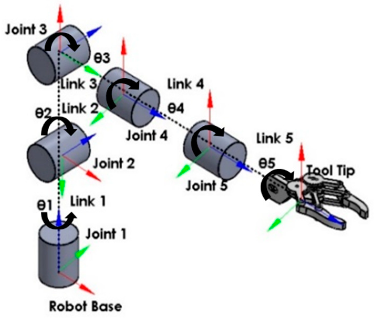
Article

A Vision-Based Bio-Inspired Reinforcement Learning Algorithms for Manipulator Obstacle Avoidance

1
Department of Electrical and Electronics Engineering, Birla Institute of Technology and Science Pilani, Dubai Campus, Dubai P.O. Box 345 055, United Arab Emirates
2
Department of Mechanical Engineering, Birla Institute of Technology and Science Pilani, Dubai Campus, Dubai P.O. Box 345 055, United Arab Emirates
*
Author to whom correspondence should be addressed.
Electronics 2022, 11(21), 3636; https://doi.org/10.3390/electronics11213636
Submission received: 23 September 2022 / Revised: 26 October 2022 / Accepted: 28 October 2022 / Published: 7 November 2022

Abstract

:
Path planning for robotic manipulators has proven to be a challenging issue in industrial applications. Despite providing precise waypoints, the traditional path planning algorithm requires a predefined map and is ineffective in complex, unknown environments. Reinforcement learning techniques can be used in cases where there is a no environmental map. For vision-based path planning and obstacle avoidance in assembly line operations, this study introduces various Reinforcement Learning (RL) algorithms based on discrete state-action space, such as Q-Learning, Deep Q Network (DQN), State-Action-Reward- State-Action (SARSA), and Double Deep Q Network (DDQN). By positioning the camera in an eye-to-hand position, this work used color-based segmentation to identify the locations of obstacles, start, and goal points. The homogeneous transformation technique was used to further convert the pixel values into robot coordinates. Furthermore, by adjusting the number of episodes, steps per episode, learning rate, and discount factor, a performance study of several RL algorithms was carried out. To further tune the training hyperparameters, genetic algorithms (GA) and particle swarm optimization (PSO) were employed. The length of the path travelled, the average reward, the average number of steps, and the time required to reach the objective point were all measured and compared for each of the test cases. Finally, the suggested methodology was evaluated using a live camera that recorded the robot workspace in real-time. The ideal path was then drawn using a TAL BRABO 5 DOF manipulator. It was concluded that waypoints obtained via Double DQN showed an improved performance and were able to avoid the obstacles and reach the goal point smoothly and efficiently.

1. Introduction

In general, industrial robots operate faster and more precisely than humans, particularly in an assembly line where robots perform repetitive tasks. Hence, to find the shortest or optimal path between two points, path-planning is an important primitive for autonomous industrial robots. Solving path planning is important for ensuring efficient robot control and obstacle avoidance [1]. Path planning cannot always be designed in advance as the global environment information is not always available a priori, especially in a complex industrial environment. By proposing a proper algorithm, path planning can be widely applied in partially and unknown structured environments where the robot can adapt to changes in the environment [2,3]. Traditional path planning requires knowledge about the environment and robots cannot learn in complex environments [4]. Hence in recent years, various methods for planning the waypoints have been developed that involve the use of artificial intelligence techniques and heuristic approaches. However, with the increasing complexity of the working environment, different obstacles of varying sizes exist [5,6,7]. So, to address the above issues, the model-free reinforcement learning approach is used for path planning where the robot generates the optimal path through trial and error in a limited workspace. The reinforcement learning algorithm uses the Markov Decision Process (MDP) where the probabilities and rewards are unknown. For this purpose, a specific function is formulated which optimizes the rewards based on the actions through trial-and-error. Moreover, reinforcement learning is majorly used in mobile robot simulations but has been less explored in manipulators with a restricted workspace because of its complexity. The methodology proposed in this work can be used for assembly line operations in industries where repeated jobs take place in a limited workspace area. To simulate the industrial scenario, an experimental environment with multiple obstacles was created where the workspace area was fixed based on the camera field of view. Further, obstacle avoidance was carried out because multiple obstacles may be encountered while performing assembly operations. The modeling of a 5 DOF manipulator is also covered as it was necessary to implement the task efficiently [8,9]. In this analysis, movement along z was not considered so as to operate the robot in safe manner. This methodology could also be extended to 3D path planning.

2. Related Works

There are many studies that have been reported in the field of path planning with both conventional and machine learning approaches but among them, machine learning approaches have gained a lot of popularity [10]. Wang et al. proposed a globally guided reinforcement learning approach (G2RL) for path planning under dynamic environments which used spatiotemporal environment information to obtain rewards [11]. Lee et al. proposed Q-Learning-based path planning for optimizing the mobile paths in a warehouse environment. The author performed various simulation tests by varying rewards based on actions and measured path length and path search time and compared the performance with the Dyna-Q learning algorithm [12]. Dong et al. proposed an improved Deep Deterministic Policy Gradient (DDPG) algorithm for the path planning of a mobile robot by adaptively varying exploration factors. The author also compared it with other reinforcement algorithms such as Q-Learning and SARSA and found that DDPG performed better with less computation time and faster convergence [13]. Quan et al. proposed Gazebo-simulated path planning of Turtlebot3 using Double Deep Q-Learning Network (DDQN) and Gated recurrent units (GRU)-based Deep Q-Learning. The authors finally compared the performance of reinforcement algorithms with conventional and heuristic algorithms, namely the A* and Ant-colony algorithm [14]. Yokoyama et al. proposed an autonomous navigation system based on the Double Deep Q-Network using a monocular camera instead of 2D LiDAR [15], whereas Farias et al. implemented reinforcement learning for position control of the mobile robot by controlling the linear and angular velocity [16]. Wang et al. reviewed various image processing techniques for weed detection. The various techniques such as color index-based, threshold-based, and learning-based ones were discussed in detail [17]. Islam et al. used shapes, color, and texture features to detect the objects in Columbia Object Image Library datasets [18] whereas Attamimi et al. used color and shape-based features as the input to the K Nearest Neighbor classifier to identify the objects for domestic robots [19].
Based on the above discussion, it can be inferred that reinforcement learning approaches have been implemented mostly for mobile robot navigation with predefined maps with obstacles. The literature available for solving path planning for manipulators using reinforcement learning in unknown environment obtained from a vision sensor is very limited. Hence the main goal of this paperwork was to implement different RL algorithms for vision-based obstacle avoidance using the camera for 5 DOF robotic manipulators in a planar environment. Moreover, to find the optimal training values, different test cases with varying hyperparameters were analyzed. To automate the process of objects detection in workspace, this paper used visual feedback information for determining the start, goal, and obstacle positions. This information was further converted into robot coordinates for tracing the path in real-time which is another contribution of this paper. The main objectives are listed below:
  • Implementation of image processing techniques to find the start, goal, and obstacle positions to be given as inputs to different RL algorithms;
  • Implementation of a homogeneous transformation technique to determine the grid world coordinates for corresponding camera coordinates and robot coordinates for respective grid world coordinates;
  • Application of different reinforcement learning algorithms such as Q-Learning, DQN, SARSA, and DDQN for path planning;
  • Optimization of training hyperparameters using Genetic algorithm and Particle swarm optimization algorithms;
  • Performance evaluation comparison by varying actions, convergence criteria, obstacle clearance, and episodes to find optimal parameters for Q- learning and noting the pat length and time elapsed for each test case;
  • Real-time online-based experimental verification for vision-based obstacle avoidance for all the test cases using the input obtained from the live camera feed.
The paper is further divided into four sections. Section 3 explains vision-based obstacle avoidance using different RL algorithms with camera calibration. This is followed by a performance evaluation of different RL algorithms in Section 4. The experimental results obtained with their performance analysis are discussed in Section 5. Finally, the conclusion and future scope of the work are discussed in Section 6.

3. Vision-Based Obstacle Avoidance Using Different Reinforcement Learning Algorithms

In this section, the uses of various reinforcement learning approaches to avoid obstacles placed in the workspace of TAL BRABO 5 DOF manipulator are studied. This manipulator has five joints, and they are named as x ,   y ,   z ,   u , and v joints. This robot is India’s first articulated indigenous robot manufactured by Tata Automation Ltd. which is used in industries for pick and place, welding, painting, assembly applications, and vision-based jobs. It helps industrial professionals from dangerous workplaces and provides an efficient operation [20]. The commands to the robot are communicated to the robot using the Trio Motion controller via the ActiveX library installed in MATLAB. The robot has a payload capacity of 10 kg with 750 mm of maximum reach. The detailed kinematic modeling is described in Appendix A.1. In a reinforcement learning scenario, the environment is the dynamic models with which the agent interacts. The environment receives actions from the agent and based on the actions it generates a reward which denotes how well the action contributes to achieving the task [21]. There are different types of reinforcement learning algorithms reported in the literature which are classified on the basis of model-based and model-free algorithms.
The model-based RL algorithm uses machine learning models such as the random forest, gradient boost, and neural networks to create a policy function whereas in a model-free environment the policy does not use any explicit models. In this work, the model-free algorithm was used because it is a simple process where policy is refined based on the actions and it does not need any environment model to maximize the reward. It does not use any probability distribution as used in the Markov Decision Process and can be viewed as a trial-and-error algorithm. The model-free is further classified as on-policy and off-policy algorithms. Q-Learning is an off-policy algorithm where the updated policy is different from behavior policy and estimates the rewards for future actions whereas in on policy the agent follows the optimal actions it has calculated [22]. SARSA is an example of an on-policy RL algorithm. Therefore, on policy can be used in the situations where the agent wants to explore, and off-policy can be used where the agent wants to exploit [23].

3.1. Image Processing for Identification of Objects in a Robot Workspace

The main contribution in this work is that the inputs to the algorithm which are the robot coordinates were obtained from transformed coordinates from the live camera feed. The start, goal, and obstacle positions were obtained as pixels and the camera to robot base transformation was implemented to obtain robot coordinates. The vision system used in this work was an eye-to-hand configuration where a single 2D Ashu HD web camera was tilted at an angle of 26° to view the robot’s workspace where the obstacles were placed. At this position the camera was calibrated by placing the checkerboard on the robot workspace as shown in Figure 1. The main goal of the calibration was to find the geometric parameters of the image formation and also it helped in eliminating distortion and skew in images.
The pattern centric and camera centric view of during the calibration process is shown in Figure 2a,b.
Once the calibration was completed, the camera frames were captured, and the RGB image was converted to grayscale and a particular channel, namely green, blue, and red channels, were extracted from the RGB data using the image subtraction technique where pixel values were subtracted to segment the particular part in the image. Once the single channel was extracted, 2D median filtering was applied to remove the salt and pepper noises present in the image and pads with zeros to preserve the edges. Further, the grayscale image was converted to black and white with the threshold values of 0.05, 0.18, and 0.1 for green (obstacles 1 and 2), red (goal), and blue (start) detection, respectively. Finally, image blob analysis was carried out to find the bounding box coordinates and centroid values of the objects in pixels. The process flow diagram for color-based detection using image processing is shown in Figure 3.
Further the image coordinates needed to be converted to grid world coordinates; hence, in this work, a simple and robust technique called homogeneous coordinate transformation was implemented to obtain the grid coordinates from equivalent obstacle pixel coordinates. The detailed explanation of homogeneous coordinate transformation can be referred to in Appendix A.2. Finally, from Equation (A7) the 4 × 4 transformation matrix was obtained. The obtained transformation matrix T c w in this work is described in Equation (1) [24].
T c w = [ 0.0014 0.0208 0 1.581 0.019 0.0014 0 1.703 0 0 0 0 0 0 0 1 ]  
Finally, using this transformation matrix, the coordinates of start, goal, and goal coordinates were transformed to real-world coordinates and fed to different RL algorithms as inputs for path planning. The overall methodology followed in this paper for vision-based obstacle avoidance is shown in Figure 4.

3.2. Path Planning Using Q-Learning

The path planning using Q-Learning in this study was explored using a robotic manipulator to avoid obstacles placed in its workspace. This work has great significance in industries where robots and humans work together where it finds the optimal waypoints under both static and dynamic environments. Q-Learning is a model-free off-policy reinforcement learning algorithm that learns the value of an action in a particular state without the environment model. Moreover, it can handle problems with stochastic transitions and rewards without requiring adaptations [25]. The common steps followed in Q-Learning-based path planning are creating the environment, calculating the reward matrix, selecting the actions, and updating the Q-table [26].

3.2.1. Creating the Environment

The reachable robot workspace considered for the analysis was (180, 126) mm. This workspace was visualized as grids of 7 × 10 for ease in simulation analysis where each grid in the simulation was equivalent to the center point of four smaller square grids of size 18 mm. Specific colors were chosen for the start, goal, and obstacle positions. The blue object was taken as start position with a grid value of (1, 1); the red object was taken as goal position with a grid value of (5, 9); the green object was taken as obstacle position with grid values of (2, 3) and (4, 8), respectively. The environment generated in MATLAB is shown in Figure 5 where Figure 5a is the simulated environment chosen for the reinforcement learning model and the real-time grid world environment is shown in Figure 5b.
From the figure, it can be seen that the grid world for the corresponding real-time workspace was created for simulation analysis. The start coordinates were always taken as (1, 1) and the goal point as (5, 9). This configuration was followed throughout the analysis. The main goal of the agent is to reach the blue block from the start position avoiding the two obstacles. When the agent encounters an obstacle, the agent takes additional jump from one state to another state as shown by the red arrow. This makes the further learning of the agent easier. By implementing different configurations of the start, goal, and obstacle positions, all possible combinations were also analyzed in further sections.

3.2.2. Action Selection and Q-Table Initialization

For every state   s , the agent takes the action a based on the interactions with the environment. Each time the action is performed, reward R is calculated before progressing to the next time step t + 1 . This entire process is divided into episodes where the agent tries to complete the goal task or run the process for fixed time steps. In this work, four main actions were taken: North = 1, South = 2, East = 3, West = 4. The Q-Learning algorithm works on the Q table which is the mapping between the states and actions. Each row represents the states and columns represent the actions. The q-table is always initialized to zero. The Q table stores the Q values of state-action pairs, and they are initially set to zero. The rows in the table represent the robot’s joint angles which is the state, and the columns represent the action corresponding to the given state [27]. With the environment and reward obtained, the Q value is calculated at each step per episode and stored as state-action pairs in the Q table. During training, the Q table is updated till the episodes are completed and converged. The updating equation for the Q table is given by,
Q ( s ,   a ) = Q ( s , a ) +   α [ R ( s , a ) + γ m a x Q ( s , a ) Q ( s , a ) ]
where α is the learning rate refers to the rate of updating the Q value. If it is set to zero, Q values are not updated and hence nothing is learnt. Hence, it is always chosen closer to 1. γ is the discount rate which reveals how much the agent has to account for for future rewards and it varies between 0 and 1. The optimal Q value function q * ( s , a ) is the maximum action–value function that is selected from each row in the Q table which signifies the maximum amount of reward that can be extracted for the current state and action. Based on this optimal q value, the best optimal route to goal point will be obtained. The optimal Q value is given by
q * ( s , a ) = m a x ( q ( s , a ) )

3.2.3. States and Rewards

The states s t are the observations that the agent receives from the environment, and they act as an interface between the agent and the environment because not every environment will provide full information to the agent. In this paperwork, the robot workspace was chosen as states with grid world coordinates varying from (1, 1) to (7, 10). The reachable workspace of robot was limited and to match the robot workspace with the camera’s field of view, the experimental test was conducted within 7 × 10 grid size.
The reward is a scalar-valued function that is used for evaluating the agent’s (robotic arm) actions. The rewards are chosen in such a way that positive rewards denote that the agent has reached the goal point and if it receives the negative reward, the agent encountered the obstacles. Here in this work, an additional reward was given when the agent reached one grid closer to the goal point so that convergence became faster and accurate. The reward R ( s ,   a ) for current state s and action, a is given by,
R ( s , a ) = { 10             , i f   g o a l   i s   r e a c h e d 5 ,                                 c l o s e r   t o   g o a l 1 ,                                                       o b s t a c l e 1 ,                                         j u m p   s t a t e
Finally, the expected value of the next reward is given by,
R ( s , a , s ) = E [ R t + 1 | s , a , s ]
where s is the next state at time t + 1 and R t + 1 is the reward at time t + 1 .

3.2.4. Updating the Q-Table

When the agent performs actions based on the interaction with the environment, it receives a reward and corresponding q values are calculated. These values are then updated in the Q table. Also in this work, ε -greedy was implemented to randomly explore the actions which help the agent (robot) learn faster and better and does not stick to the local minima [28]. In general, the ε -greedy policy adopts the best selection from candidates with the probability of ε and a random selection with the probability of 1 − ε . The value of ε determines the probability with which the agent performs a random action [29]. If a random action generated is lower than the value of ε , the agent is allowed to take random actions, or else the action is determined by the model. As the episodes increase, the value of ε decreases slowly from 1 [30]. For this work ε was chosen to be 1 since the agent was allowed to explore rather than perform greedy exploitation. The general equation for ε -greedy policy is as follows,
a = { M a x q t ( a )                             w i t h   p r o b a b i l i t y   1 ε A n y   a c t i o n   a                               w i t h   p r o b a b i l i t y   ε

3.3. Path Planning Using SARSA

State-Action-Reward-State-Action (SARSA) is a model-free on policy algorithm where the Q-value depends on the current state of the agent a , the action the agent chooses a , the reward R the agent obtains for choosing this action, the next state s that the agent enters after taking that action, and finally the next action a the agent chooses in its new state. The environment, states, actions, and rewards for path planning are the same values that were discussed previously. The SARSA agent interacts with the environment and updates the policy based on actions taken [31]. The Q value for a state-action pair is updated by an error, adjusted by the learning rate α. The updating equation is given as,
Q ( s ,   a ) = Q ( s , a ) + α [ R ( s , a ) + γ max Q ( s , a ) ]
The major difference between Q-Learning and SARSA is that in QL, when the reward passes from the current state to the next state, it takes the maximum possible reward of the new state and takes random actions whereas in SARSA it follows the obtained policy and takes current action. The SARSA algorithm can be used when the agent wants to explore whereas Q-Learning can be used when the agent does not want to explore the environment [32].

3.4. Path Planning Using DQN

DQN is also a model-free RL algorithm where the modern deep learning technique is used. DQN algorithms use Q-Learning to learn the best action to take in the given state and a deep neural network or convolutional neural network to estimate the Q value function [33]. The state is given as the input and the Q-value of all possible actions is generated as the output. In this work, Long Short Term Memory (LSTM) which is one of the Recurrent Neural networks was used as a function approximator to map the states and actions instead of Q table. The DQN uses the Bellman equation to update the q value and it is given by
Q ( s ,   a ) = [ R ( s , a ) + γ m a x Q ( s , a ) Q ( s ,   a ) ]
In DQN, all the past experiences are stored in memory and the next action is taken based on the max q value [34]. The loss function is nothing but Mean Square Error (MSE) which is the difference between the target q value and the actual q value. R ( s , a ) + γ max Q ( s , a ) represents the target q value. The DQN architecture is built with one input neuron for states, 24 hidden neurons, and four output neurons for actions and it is shown in Figure 6. The network was further trained, and the performance was analyzed by the varying learning rate, discount factor, episodes, and steps per episode. The batch size was fixed to 64 with an L2 regularization factor of 1 × 10⁻⁴.

3.5. Path Planning Using Double DQN

The Double DQN has two neural networks where one network is used for experience replay similar to working of DQN and another neural network called target network is used to calculate the q value [35]. Here the best action a with the highest q value is obtained from the main model and for the obtained best action q, q value is estimated using the target network. Next, the q value of DQN is updated based on the estimated q value from the target network Q t n e t and the process repeats till the episodes finish. Here there is no learning rate α when updating the Q-values since it will be used in the optimization stage of DQN [36]. The basic updating equation for double DQN is as follows,
Q D Q N ( s ,   a ) = R ( s , a ) + γ Q t n e t ( s , a )
where
a = m a x   Q q n e t ( s , a )     ;     [ from   DQN ] q e s t   = Q t n e t ( s , a )   [ from   Target   network ]
Here the environment, states, actions, and rewards for path planning are the same values that were discussed previously in the Q-Learning section.
Finally, once the optimal waypoints are obtained from Q-Learning, SARSA, DQN, and Double DQN, the waypoints in terms of grid world coordinates ( x , y ) are further transformed into robot coordinates ( X , Y , Z ) and are sent to the TAL BRABO manipulator for real-time tracing using the ActiveX library in MATLAB. The transformation matrix T obtained to convert grid coordinates into robot coordinates is given by,
T = [ 15.316 10.105 0 523.594 9.837 14.784 0 2.932 0 0 0 0 0 0 0 1 ]

4. Performance Analysis of Different Reinforcement Learning Algorithms

In this section the performance of different reinforcement learning algorithms implemented in this paperwork is discussed. The training hyperparameters namely episodes, steps per episode, learning rate, and discount rate were varied randomly and for each case the length of the optimal path obtained from reinforcement algorithms and the elapsed time to reach the goal point were calculated [37]. Furthermore, analysis was extended to apply PSO and GA for optimizing the training hyperparameters instead of randomly varying the training parameters. Moreover, performance for path planning using optimal parameters was compared with standard random values and also implemented in real-time experimentation. The detailed performance analysis implemented in this work is shown in Figure 7.
The length of the path was calculated based on the Euclidean Distance calculated between two points at every step progressing towards the goal point. Moreover, the elapsed time was calculated which reveals how long the agent has taken to reach the goal point [38]. In reinforcement learning, during each episode, the sequence of states, actions, and rewards varies from the initial state to the terminal state to maximize the rewards; hence, it is one of the important training parameters considered for performance analysis. The next parameter which is varied is the steps per episode which denote the number of steps or iterations per episode.

5. Results and Discussion

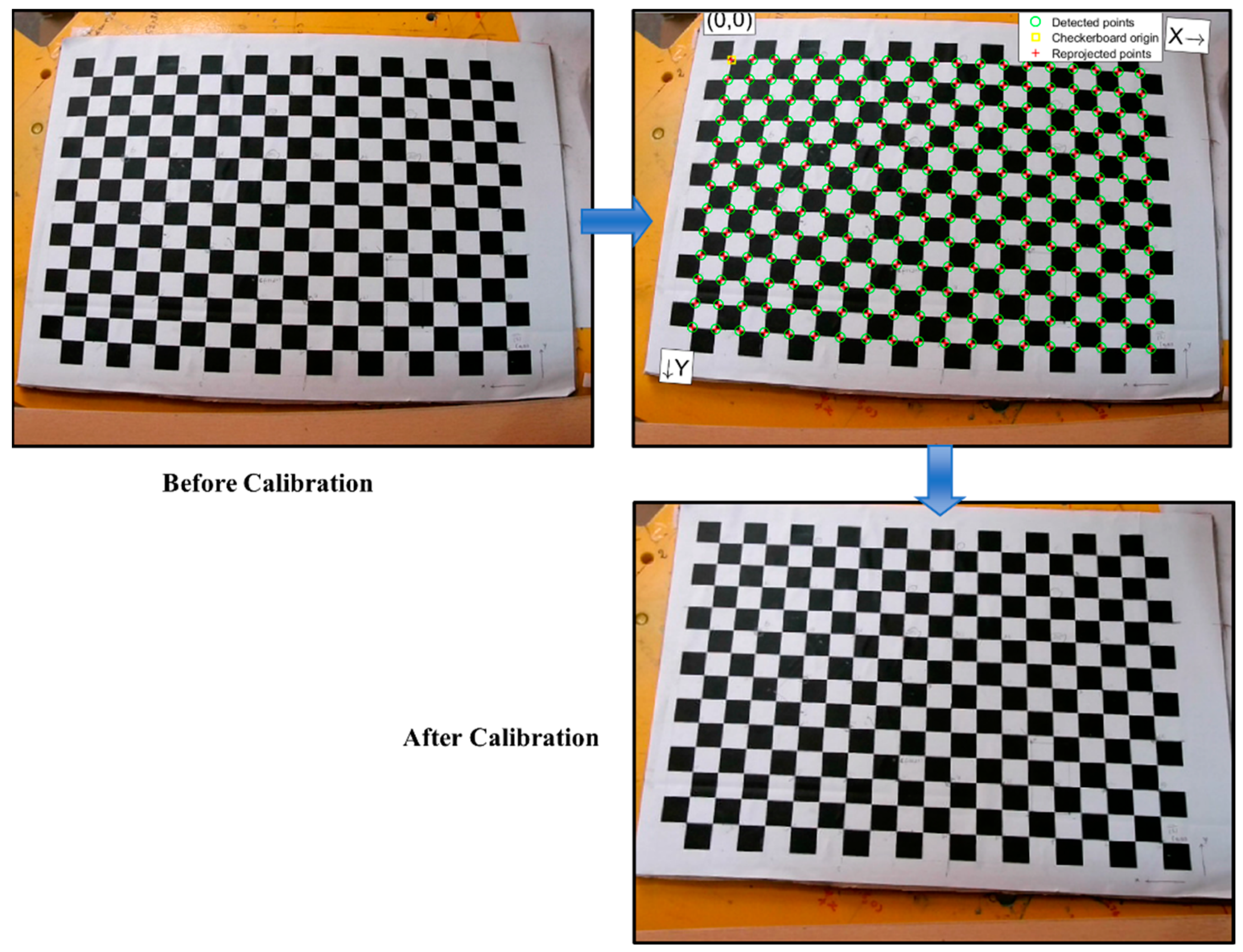
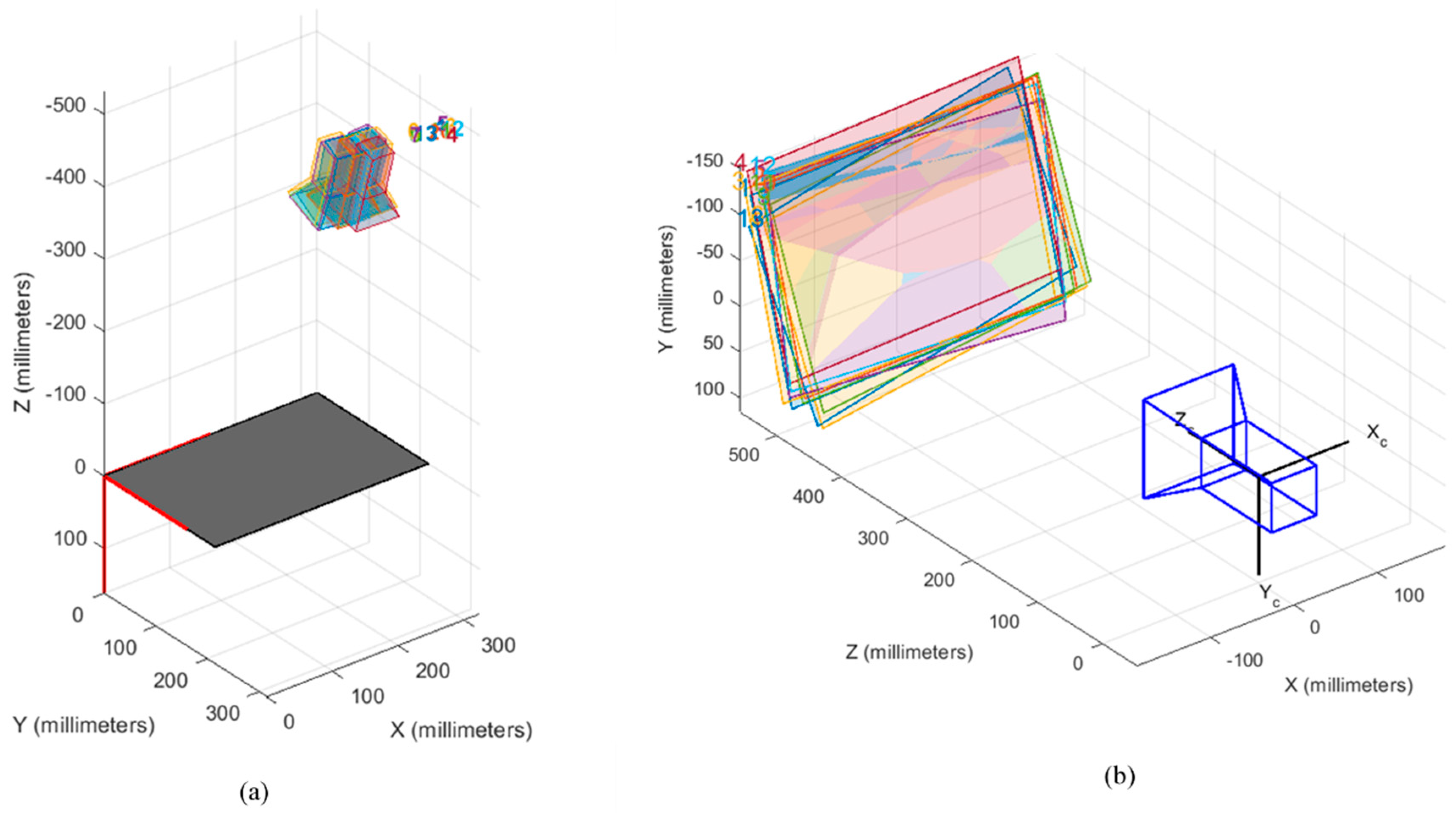
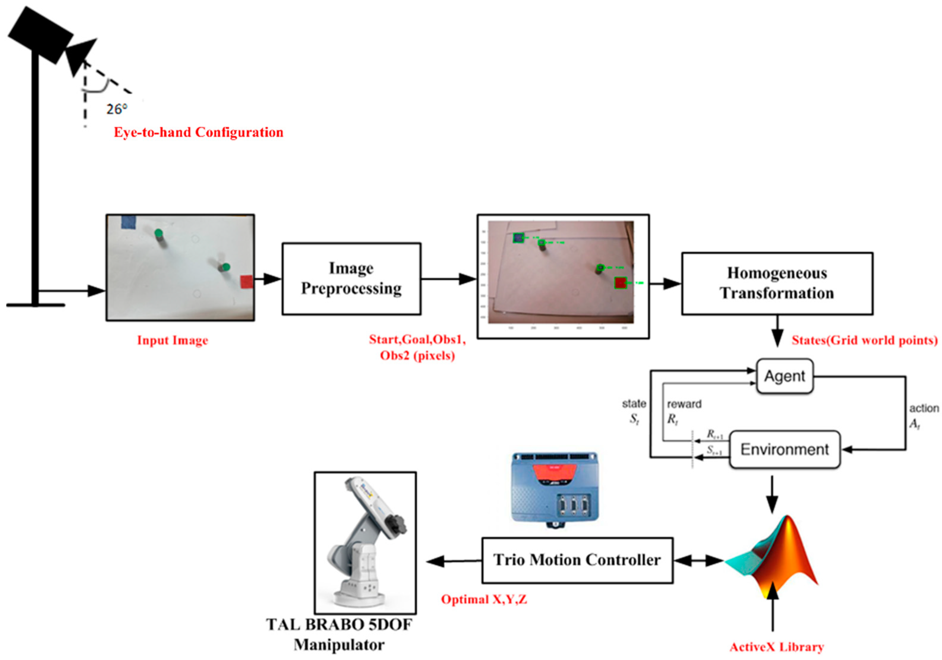
This section presents various results obtained for different test cases for different reinforcement learning algorithms. Their performance was compared, and an optimal set of parameters was chosen for real-time experimentation using TAL BRABO manipulator. The experimental setup for performing vision-based path planning and obstacle avoidance is shown in Figure 8.
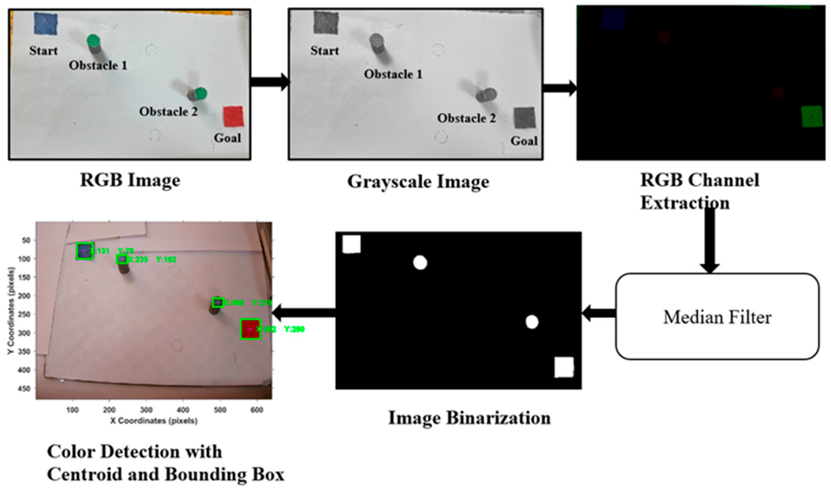
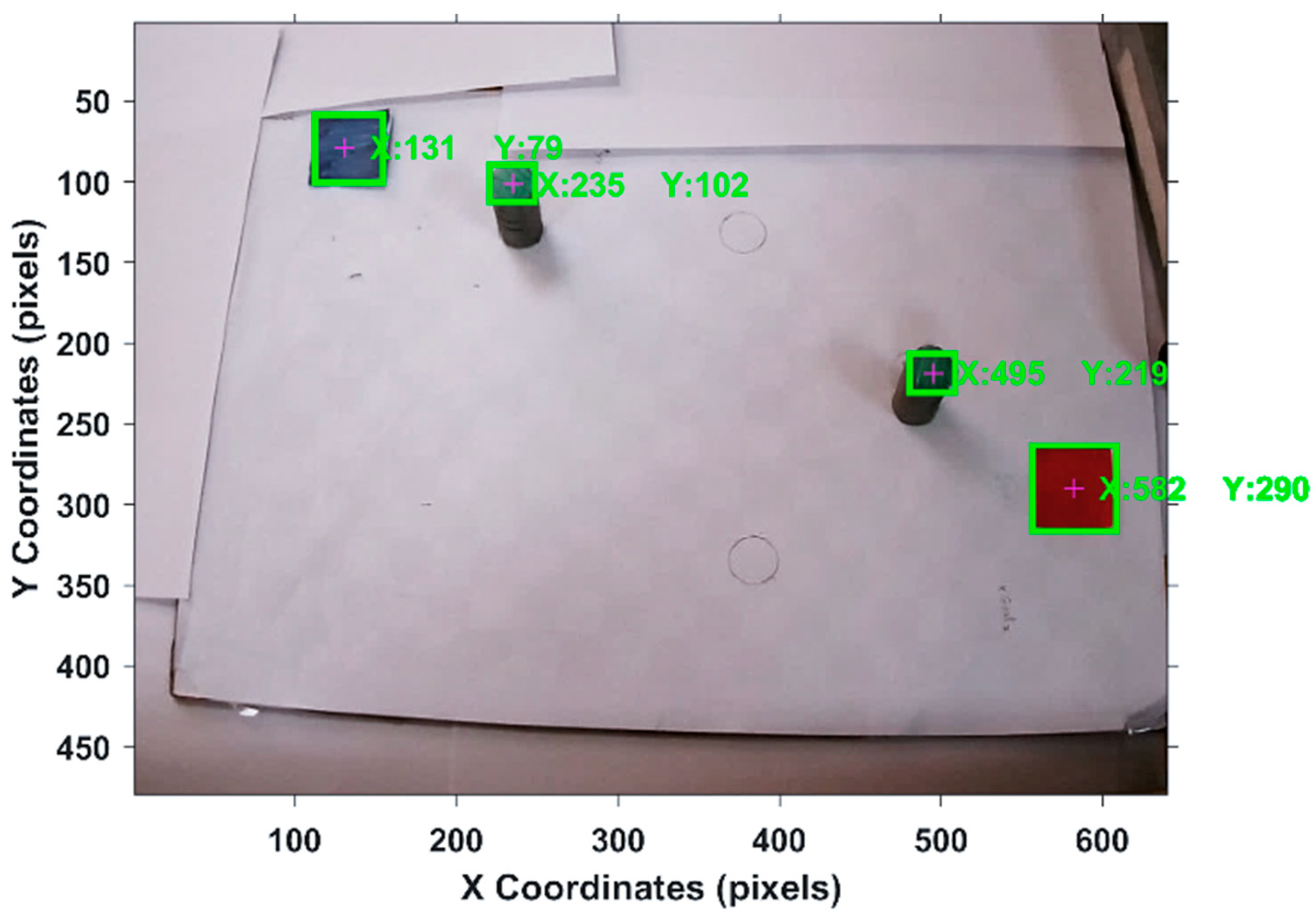
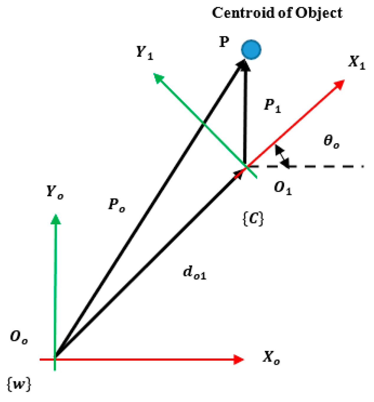
The camera captured the workspace where obstacles were kept and using image processing the colors were segmented and contours and a centroid were drawn over each object. Using the centroid values, corresponding grid world coordinates were obtained using the transformation matrix specified in Equation (8) and fed as input to the reinforcement learning algorithms. The live camera feed capturing the objects placed in the workspace is shown in Figure 9 and their pixel, grid values, and their robot coordinates are tabulated in Table 1. The robot coordinates were obtained from Equation (A7) as described in Appendix A. With the increase in episodes, a better optimal policy can be obtained which leads to better learning. Since the grid world was smaller, episodes of 5000 performed better but based on the environment the episodes needed to be adjusted for better performance. Next, the average rewards were analyzed, and it was seen that the one with a lesser average reward performed better because there was less deviation between the reward given and what the agent received. When the deviation was large, the agent was not able to reach the goal point.
Once the transformed coordinates were obtained, using these parameters, different reinforcement learning algorithms were trained for different episodes namely 1000, 3000, and 5000. The steps per episode were varied as 50, 100, and 300. The learning rate was chosen as 0.0001, 0.2, and 1, whereas the discount rate was chosen as 0.01, 0.5, and 0.99. All these parameters were chosen in such a way that they had low, medium, and high values. Finally, by using different combinations, the length of the path traversed, average reward, average steps per episode, and time taken to reach the goal were calculated for different RL algorithms. Here, the consolidated results of average path length for different reinforcement learning algorithms are tabulated in Table 2 and the detailed table is described in Table A2 under Appendix A.2.
Since the environment was very small for path planning, the maximum episodes were taken as 5000 and steps per episode as 300. It was also observed that with episodes more than 5000, the performance was poor, and the path generated was noisy. From the above table, it can be noted that during the experimental analysis, when the episodes increased from 1000 to 5000, the total elapsed time taken by the agent to reach the goal point also increased. Further, there was no change in path length for all the algorithms and this was the same for different episodes and learning rates. The notable difference in path length was observed while varying the discount factor as this is the important weighting factor which determines the importance of rewards for the future states. From the above analysis, Double DQN was able to reach the goal point exactly with the path length of 216.07 mm while Q-Learning and SARSA were not able to reach the goal point with 5000 episodes. The average steps and elapsed time for training the agent are tabulated in Table 3 with 5000 episodes, 300 steps per episode, the learning rate of 1, and the discount rate of 0.99.
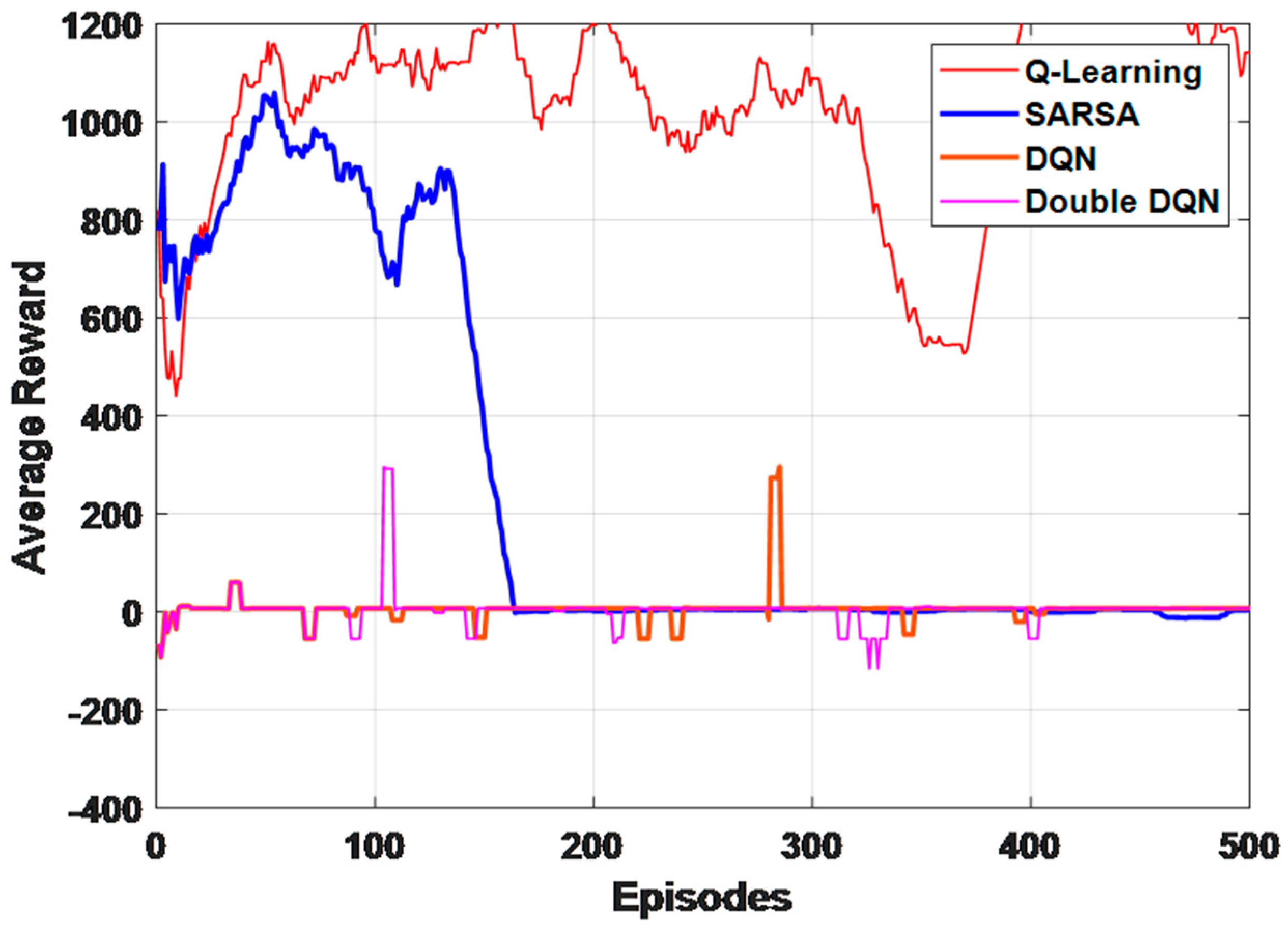
The above table discusses the average steps and total time taken for training for different algorithms in which steps taken by double DQN was less with the value of 10.4 which shows that training converged with the values equal to the stopping criteria whereas Q-Learning had average steps of 206.7. Q-Learning took 2387.2 sto complete the training whereas SARSA completed the training within 2073.9 secs (35 min). Moreover, it was noticed that training was faster with SARSA than any other algorithms. The DQN algorithm took 3957.4 s which is approximately one hour for training which was much slower compared to others. Among deep reinforcement learning algorithms, performance was better for double DQN since it simultaneously ran the DQN for experience replay and calculated the q value using another network whereas in DQN, the Q-value was updated using the reward in the next state. The convergence comparison of different algorithms with respect to the first 500 episodes with a learning rate of 1 is illustrated in Figure 10. This graph provides an overall idea of which algorithm performance was better as faster convergence is needed.
From the graph, it can be seen that Double DQN converged faster within 40 episodes whereas Q-Learning performed worse since it never seemed to converge. Secondly, DQN and SARSA also converged faster at 150 and 170 episodes, respectively, compared to Q-Learning. It can be inferred that Double DQN performed better among all. 
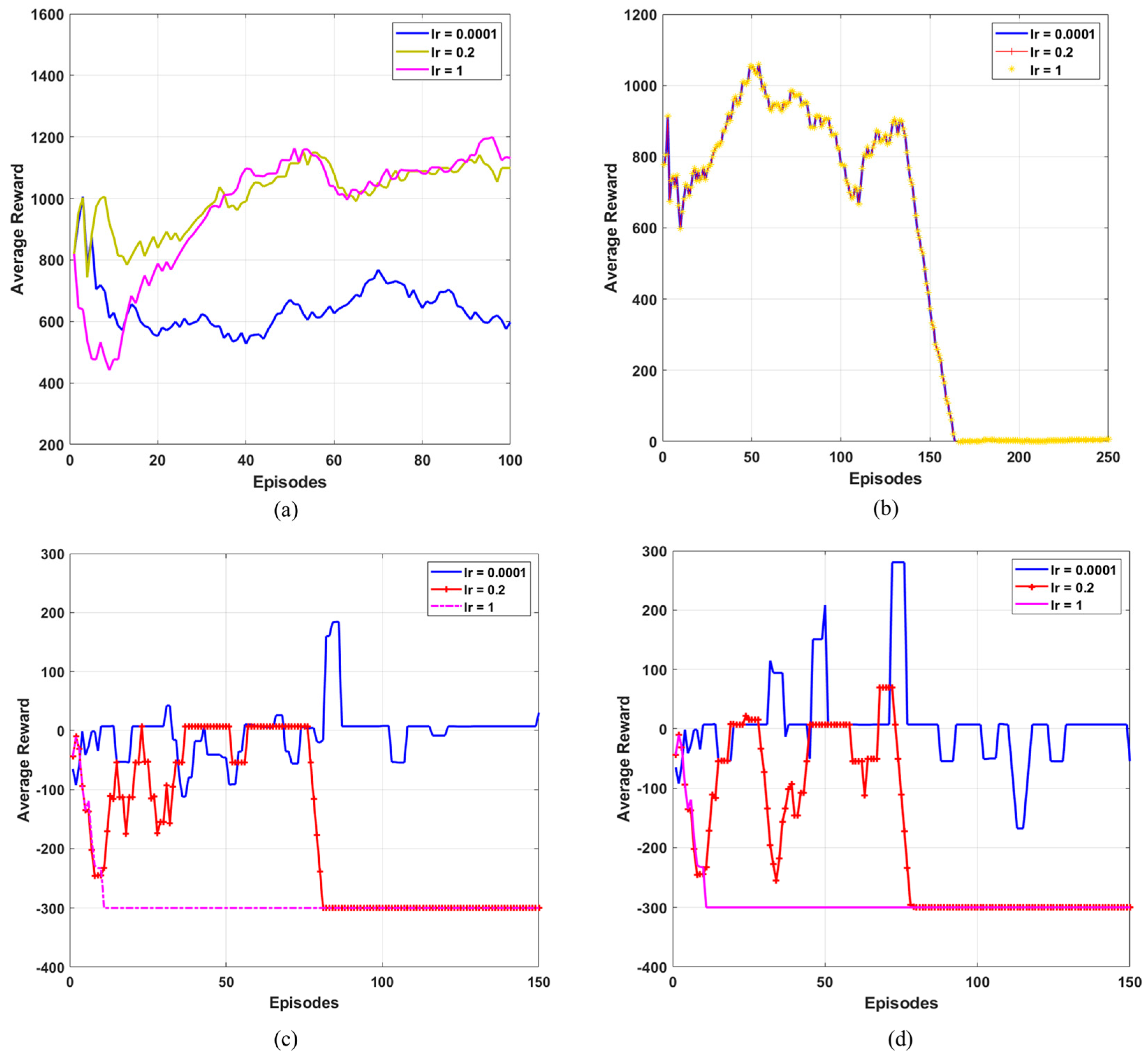
Figure 11a–d depicts the average reward obtained with different learning rates such as 0.0001, 0.2, and 1 for different RL algorithms. It was inferred that the average reward of Q-Learning varied without converging to a specific value but the average reward of SARSA took 155 episodes to converge. However, for DQN and Double DQN it converged within 85 episodes. This shows that the convergence speed was faster for the deep learning-based Q network.
Further, 
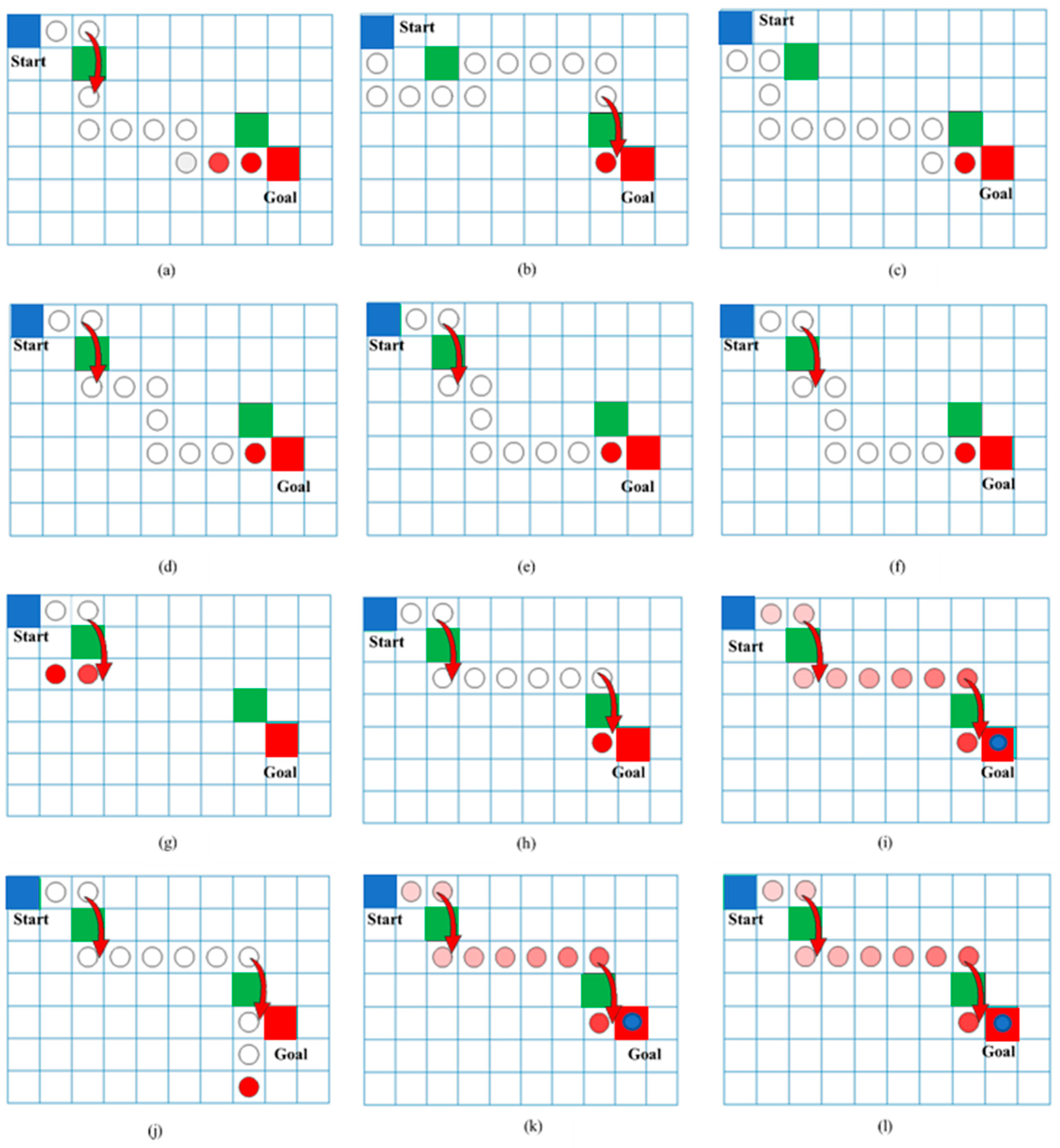
Figure 12a–c denotes the different optimal paths taken by the agent for Q-Learning for steps 50, 100, and 300, respectively. Similarly, Figure 12d–f shows the agent path using SARSA for 50, 100, and 300 steps, respectively. Figure 12g–i describes the path using DQN for 50, 100, and 300 steps, respectively and finally Figure 12j–l shows the path obtained from Double DQN for 50, 100, and 300 steps, respectively. The agent tries to reach the goal point by moving from one grid to another by trial-and-error during learning process. When it encounters an obstacle, a jump is made from one grid to another to find the optimal path in less time which is denoted by red arrow. Here in this paperwork, the agent movement around the obstacle was recorded which could be further used for calculating the probabilities of the future states. The transition jump around the obstacle was taken as 1 and other surrounding grids were made zero so that it did not visit that grid because it was seen that when it reached nearby grids, time to reach goal was more and sometimes it did not reach the goal. Then it was seen that Q-Learning and SARSA were not able to reach the goal point exactly but reached the grid before the goal point which approximated to an 18 mm difference in robot workspace. However, DQN and Double DQN performed better and reached the goal point exactly, which showed that deep reinforcement learning performed better than conventional reinforcement learning algorithms. Hence, steps per episode played a major role as they recorded the state and reward for the state–action pair.
Next by varying the discount rate, the agent’s path was recorded, and its performance was compared. The discount rate considered in this work was 0.01, 0.5, and 0.99, respectively. This is one of the important weighting factors for reinforcement learning apart from learning rate since it reveals the importance of future rewards and adjusts the agent’s behavior accordingly for long-term goals. So, the agent path was recorded which is illustrated in Figure 13. Figure 13a–i denotes the different paths taken by the agent for discount rates of 0.01, 0.5, and 0.99, respectively, using different reinforcement learning algorithms such as Q-Learning, SARSA, DQN, and Double DQN. It can be seen that for the higher discount rate, the agent was able to reach the goal efficiently but when the discount rate was 0.01 it never reached the goal, and the learning was poor. It was seen that SARSA reached the goal only when the discount rate was 0.5. Hence, the discount rate of 0.99 should be chosen for a better performance. The total agent steps generated for 5000 episodes with 300 steps per episode are tabulated in Table 4. This shows the total steps the agent took to reach the goal point.
From the table, it can be inferred that Double DQN took only 3, 80, 299 agent steps to reach the goal point whereas Q-Learning took 12, 27, 734 steps to reach the same goal point. Hence it can be concluded that Double DQN had a superior performance. Further, to find the optimal training hyperparameters, GA and PSO were implemented in this work using MATLAB. The four main input variables considered for optimizing were episodes, steps per episode, learning rate, and discount rate as these variables had a major effect on q value and rewards, and the output variables were chosen as the length of the path traversed by the agent. The GA was run with an initial population size of 50 and 400 generations. The initial swarm matrix for PSO was taken to be 0.5. The lower bound and upper bound values are shown in Table 5.
The problem was formulated as an unconstrained nonlinear optimization problem. Similarly, a particle swarm optimization algorithm was also used to compare the optimized results of GA and PSO and their effect on agent path traveled. In PSO, the swarm size was taken to be (100, 40) with an initial swarm span of 2000. The total iterations were chosen to be 800. The initial weights of each particle with respect to the neighbors’ particles were taken as 1.49. The optimized parameters were obtained from GA and PSO and one of the solutions is listed in Table 6. Finally, these parameters were implemented on different reinforcement learning algorithms, and the paths traced were analyzed.
The above discussion was entirely tested in the same environment. Further, to validate the optimized parameters obtained, in this work different environments were created and the agent actions were analyzed using the Double DQN algorithm. Since based on the above analysis Double DQN had the better performance comparatively, it was chosen for further analysis as shown in Figure 14a–d. The environment was created by adding more obstacles, changing the obstacle positions, and changing the goal point. The analysis was tested with a maximum of four obstacles using the Double DQN algorithm since this gave a better performance than the other RL algorithms.
From the Figure 14a–d, it can be inferred that the agent was able to reach the goal point under for two and four obstacles. There was some lag in reaching the goal point with three obstacles. The optimal parameters used for this analysis were, namely, episode = 5000, steps = 300, learning rate = 1, and discount rate = 0.99. Since the environment was smaller, the number of obstacles was restricted to four. These training parameters can vary based on the size of the environment and the type of applications chosen. This analysis can be implemented with similar environments and different obstacle sizes. Further, the grid world coordinates were converted to robot coordinates using the transformation Equation (A7) to perform real-time vision-based path planning. The agent path traced in terms of robot coordinates is illustrated for different obstacles and different goal points in 
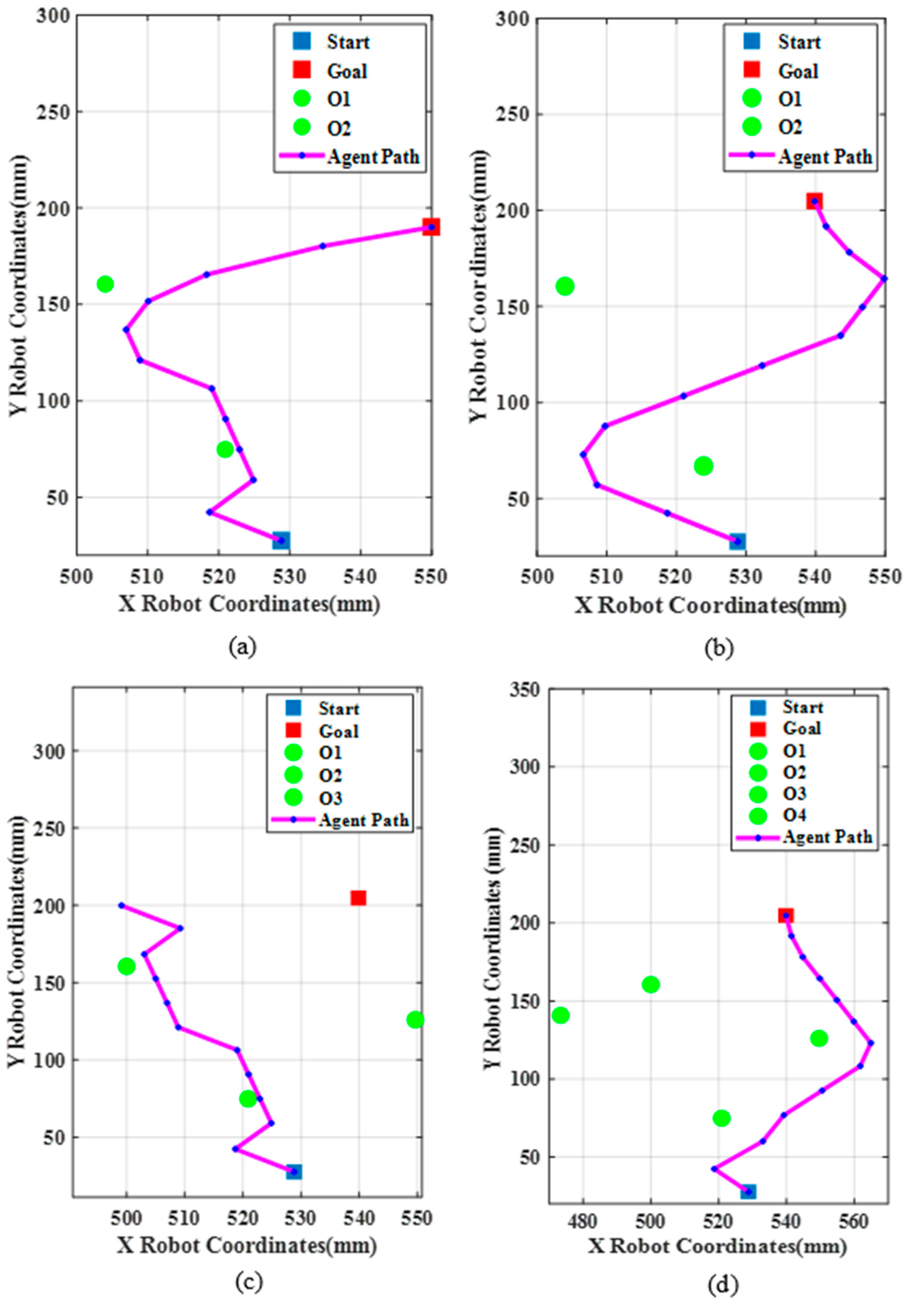
Figure 15a–d. This was analyzed to compare the simulation and real-time robot tracing.
From Figure 15a,b, the agent was able to reach the goal by the learning process with a path length of 198.16 mm and 252.47 mm. The time taken to reach the goal point was 1455.2 and 1672.66 s, respectively. Next with three obstacles, the robot was made to reach the goal, but the robot was not able to reach the goal point and had an error of about 40 mm along x and 4 mm along y from the goal point as shown in Figure 15c. The path length was 233.97 mm. Figure 15d shows the robot’s shortest path with four obstacles with a path length of 252.47 mm. It can be inferred that reinforcement learning algorithms work for any number of obstacles with suitable selection of training parameters. The obstacle considered in the simulation was a square with each side measuring 36 mm but in real time the diameter of the obstacle was 20 mm. Hence, there was a safe distance of 16 mm which was considered in the simulation analysis. The optimal training parameters obtained from GA and PSO were implemented in real-time path planning. The coordinates obtained after coordinate transformation were then sent to the robot via the ActiveX library installed in MATLAB to perform the path planning. In the real time experimentation, x and y coodinates were considered and sent to the robot with z coordinates maintained at a constant 300 mm. The reason was that for a safer operation of the z 
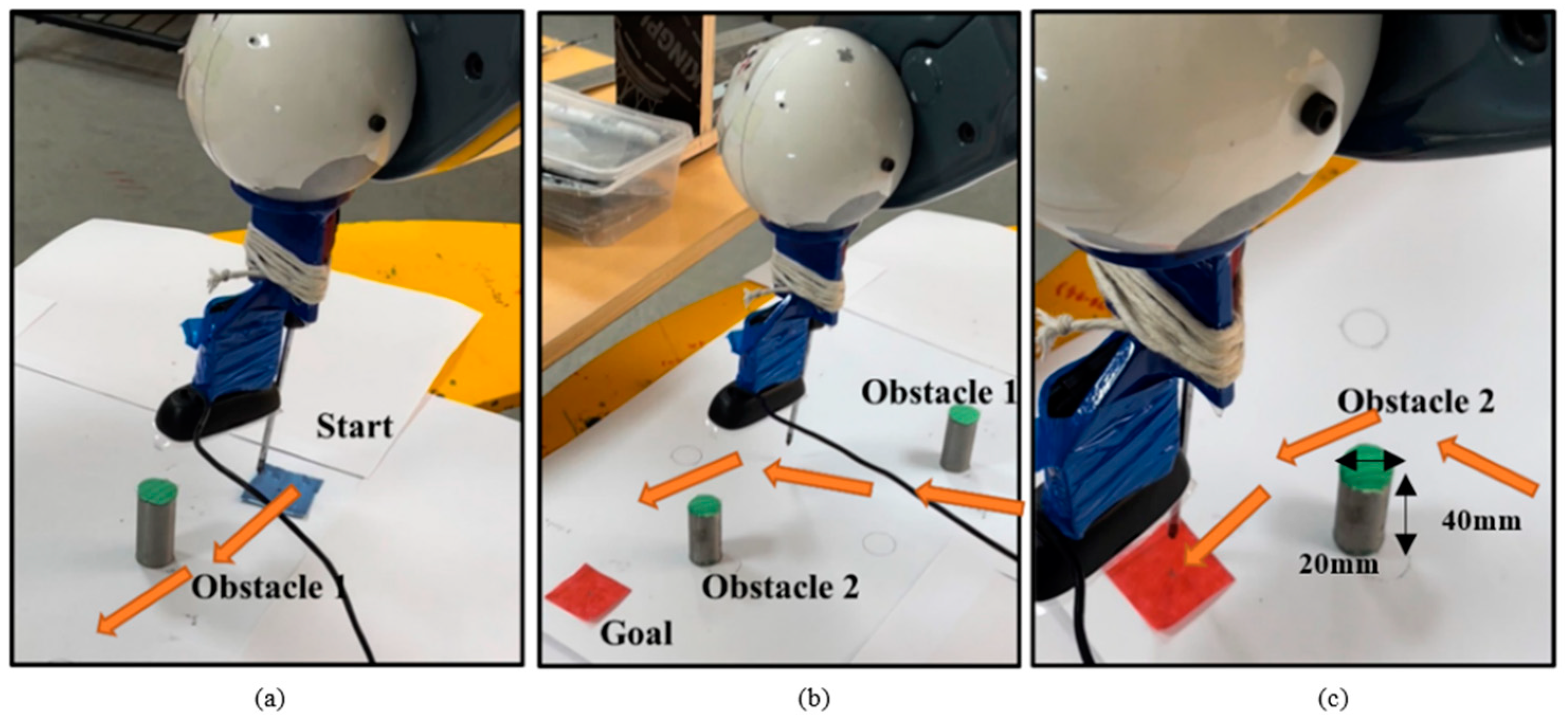
axis motors of the robot, the analysis was considered in a planar environment but in future, a 3D analysis will be considered. The real-time path planning using TAL BRABO 5 DOF manipulator with two obstacles (Figure 15b) is shown in Figure 16a–c.
From the Figure, it can be visualized that the robot tried to follow the path as illustrated in Figure 15b with two obstacles. The robot started from start position (528.805, 27.553) mm as shown in Figure 16a and tried to avoid the two obstacles as shown in Figure 16b and successfully reached the goal point (539.86, 204.84) mm as shown in Figure 16c. Similarly, the analysis was tested for other conditions with different obstacles and the robot reached the goal point without hitting the obstacles. The speed profile and joint velocities of the TAL BRABO robot while performing online path planning were recorded for case b and shown in Figure 17a,b.
The above figure shows the linear speed profile and angular velocity generated for the TAL BRABO robot with two obstacles using Double DQN. The velocity was generated for the path illustrated in Figure 17b to show that the variation of the joint velocities was very minimal while performing path planning. Thereby it shows that the use of Double DQN online-based path planning was smooth.

6. Conclusions

This work mainly focused on vision-based path planning in a robotic manipulator using different reinforcement learning algorithms such as Q-Learning, SARSA, DQN, and Double DQN and found out the optimal training parameters using GA and PSO. This work could be used in industries where humans and robots work together such as welding, assembly operations, spray painting, and so on. In this work, an industrial scenario for obstacle avoidance based on camera input was implemented for robotic manipulators. This work created a map with obstacles based on images captured from the camera for path planning. The robot workspace was divided into 7 × 10 grids (260 × 370) mm for ease of analysis and obstacles were placed occupying one grid. The grids of start, goal, and obstacles were differentiated into colors. The image processing techniques were applied successfully and using coordinate transformation, pixel to grid world coordinates were obtained. The transformed coordinates were the inputs to the reinforcement algorithms.
The following conclusions drawn from this work are as follows:
  • Performance analyses were carried out to understand the agent’s behavior by changing the important training parameters such as steps, episodes, learning rate, and discount rate;
  • Q-Learning and SARSA were not able to reach the exact goal point and had a 50 mm error from the goal point in robot coordinates. Q-Learning took 12, 27, 734 steps in total to reach the goal point, but SARSA took fewer steps of 6, 41, 319. Moreover, the SARSA convergence speed was very fast with different learning rates. Among Q-Learning and SARSA, SARSA training and performance were better and faster. SARSA performed better only with a learning rate of 0.5;
  • Deep reinforcement learning techniques such as DQN and Double DQN were also implemented in this work. It was found that Double DQN convergence was faster than DQN and it took 3, 80, 299 agent steps to reach the goal point. Among the two, Double DQN performed much better. The order of performance was as follows;
  • Double DQN > DQN > SARSA > Q-Learning;
  • The analysis with different obstacles and goal points was carried out using Double DQN as it performed better and it was found that the agent took a longer path to reach the goal point; hence, 5000 episodes was not enough for convergence. However, with four obstacles, since it took the shortest path, it reached the goal point effectively;
  • The speed profile and individual joint velocities were calculated to show the effectiveness of online-based real-time path planning using reinforcement learning algorithms;
  • Finally, the robot coordinates obtained from the grid world to robot transformation were sent to TAL BRABO Robot for real-time path planning.
This work could be further extended with dynamic objects in the robot workspace which will be the future scope of work. Moreover, different cluttered scenes could be created and the performance of the RL algorithms could be analyzed. This work focused on algorithms with discrete action space but algorithms with continuous action space could be implemented. Moreover, deep learning could be used to identify the objects in the robot workspace.

Author Contributions

Writing—original draft preparation, A.S.; methodology, A.S. and M.S.; Conceptualization, V.K. and R.K.; software, A.S. and M.S.; validation, M.S. and A.S.; investigation, V.K. and R.K; data curation, A.S.; writing—review and editing, V.K.; visualization, V.K.; supervision, R.K.; formal analysis, R.K. All authors have read and agreed to the published version of the manuscript.

Funding

This research received no external funding.

Institutional Review Board Statement

Not applicable.

Informed Consent Statement

Not applicable.

Data Availability Statement

Not applicable.

Acknowledgments

The authors are immensely grateful to the authorities of Birla Institute of Science and Technology Pilani, Dubai campus for their support throughout this research work.

Conflicts of Interest

The authors declare no conflict of interest.

Appendix A

Appendix A.1. Kinematic Modeling of TAL BRABO Manipulator

The calculation of forward and inverse kinematics of the manipulator involves the formation of Denavit-Hartenberg (DH) parameters based on reference frames drawn on each of the joints [19]. The frames of the individual robot joints of the TAL BRABO manipulator with respect to the camera frame were formulated based on DH parameters are listed in Table A1.
Table A1. DH Parameters of TAL BRABO Manipulator.
Lαd θ
0−90 0.463   [ d 1 ] θ 1
0.376   [ L 2 ]00 θ 2 − 90
0.42   [ L 3 ]00 θ 3 + 90
0−900 θ 4 − 90
000 θ 5
The DH parameters are formed based on L ,   α ,   d , and θ where L denotes the robot link length along z n 1 to z n the axis of the robot; α is the robot joint angle between z n 1 and z n axis; d is the robot link length along x n 1 to x n axis and θ is the robot joint angle between x n 1 and x n axis; n denotes the number of frames in the robot [20]. The coordinate frames of each joint were measured physically and designed in SolidWorks which is shown in Figure A1. The position and joint limits of the TAL BRABO manipulator are listed in Table 2.
Figure A1. Kinematic Diagram of TAL BRABO Manipulator.
Electronics 11 03636 g0a1
Next by using the general transformation equation as shown in Equation (A1), the transformation matrix of individual joints was formed. The general transformation equation is as follows [17],
T i i 1 = [ C θ S θ C α S θ S α L C θ S θ C θ C α C θ S α L S θ 0 S α C α d 0 0 0 1 ]
where i is the no. of frames varying from 1 to 5 for TAL BRABO; c o s ( x ) is written as C x and s i n ( x ) as S. Here x is nothing but θ   o r   α . Further using Equation (A1) individual joint transformations are formed and the final end effector to base transformation is obtained by multiplying all the matrices and it is given by
T 5 0 =   T 1 0   ×   T 2 1   ×   T 3 2   ×   T 4 3   ×   T 5 4
T 5 0 = [ 0 0 1 0.420 0.0175 0.9998 0 0 0.9998 0.0175 0 0.840 0 0 0 1 ]
From Equation (A3), last columns denote translation vector which gives ( X , Y , Z ) coordinates of the robot and for TAL BRABO it is ( 420 , 0 , 840 ) mm which is the home position of the robot.

Appendix A.2. Homogeneous Transformation of TAL BRABO Manipulator

Here grid to world transformation T g w and the world to camera transformation T w c can be obtained from camera calibration. The camera to world transformation T g c is unknown in eye-to-hand configuration. The transformation equation is as follows
T w c   T g w =   T g           c    
Next, to find the world coordinates with respect to camera pixel points, a transformation equation is formulated to represent centroid pixel point ‘ P ’ from camera frame { c } to world frame { w } as shown in Figure A2.
Figure A2. Transformation of Centroid Points P from Camera Frame to Grid World Coordinates.
Electronics 11 03636 g0a2
From the Figure A2, to align the centroid P with grid world, first, it has to be rotated by an angle of θ o and then translated by a distance of d o 1 [24]. Next, the transformation matrix is formulated from which camera to world transformation can be found out for all the camera pixel points. The equations are as follows,
[ P c 1 ] = [ R c w + d o 1 1 ] = [ R c w d c w 0 T 1 ] [ P 1 ]
In general,
P 0 = T c w   P  
Therefore, from Equation (A6) we obtain
    T c w = P 0 P 1
where P 0 is 4 × m grid coordinates with respect to the grid world coordinates; P is 4 × n camera coordinates with respect to world coordinates;   T c w is 4 × 4 transformation matrix between camera and grid world;   R c w is a 4 × 4 rotation matrix between camera and grid world;   d c w is the translation distance between camera and grid world. In this work for the formation of P c matrix, the pixel values of the robot workspace are obtained so that the entire workspace can be mapped globally. This helps in finding the robot coordinates when the objects are kept anywhere in the workspace.
The analysis based on different combinations of length of the path traversed, average reward, average steps per episode, and time is taken to reach the goal were calculated for different RL algorithms. The various results obtained are tabulated in Table A2, Table A3 and Table A4. Since the environment is very small for path planning, the episodes were taken as 5000 and steps per episode as 300. For larger environments, learning will be better if the episodes are high. From the table, it can be also noted that when the episodes increased from 1000 to 5000, the total elapsed time taken by the agent to reach the goal point also increased.

Appendix B

Table A2. List of Mathematical Symbols Used.
SymbolsMeaning
L robot link length along z n 1 to z n
αrobot joint angle between z n 1 and z n axis
d robot link length along x n 1 to x n axis
θ robot joint angle between x n 1 and x n axis
T i i 1 Transformation matrix between i frame and i 1 frame
C x cos ( x )
S x s i n ( x )
( x , y ) Grid world Coordinates
( X , Y , Z ) Robot Coordinates
s Current state at time t
a Current action at time t
R Current Reward at time t
α Learning rate for RL algorithms
γ Discount rate for RL algorithms
Q D Q N ( s ,   a ) Q value of Double DQN network
Q q n e t ( s ,   a ) Q value of DQN network
Q t n e t ( s ,   a ) Q value of target network
Table A3. List of Abbreviations.
AcronymAbbreviations
RLReinforcement Learning
DQNDeep Q Network
SARSAState-Action-Reward-State-Action
DDQNDouble Deep Q Network
MATLABMATrix Laboratory
TALTata Automation Ltd.
DOFDegrees of Freedom
DHDenavit-Hartenberg
Table A4. Performance Evaluation of Different reinforcement Learning Algorithms.
ParameterAlgorithmValuesLength of PathAverage RewardAverage StepsTime (s)ParameterAlgorithmValuesLength of PathAverage RewardAverage StepsTime (s)
EpisodesQ-Learning1000198.161286.3270.8553.19Steps/EpisodeQ-Learning50234.57174.7649.73970.71
3000198.161160.9244.131419.1 100198.16376.888.961305.2
5000198.161104.8206.72387.2 300198.161104.8206.72387.2
SARSA1000198.16617.2134.4285.76 SARSA50198.16182.3647.5902.93
3000198.16568.4124.9852.78 100198.16556.66122.41455.2
5000198.16556.66122.41455.2 300198.161143.26240.332073.9
DQN1000216.07710301.79 DQN5090.131−50502102.6
3000234.57−110.43002211.4 100233.98715.6191.43844.3
5000216.07228.854.63957.4 300216.07228.854.63957.4
Double DQN1000216.07710321.4 Double DQN50348.0812646.62305.8
3000216.076.810.21022.9 100216.07−34.4483955
5000216.076.610.43735.1 300216.076.610.43735.1
Learning rateQ-Learning0.0001198.16902.93208.32335.7Discount FactorQ-Learning0.0117.9−214.33288.632818
0.2198.16898.23224.52351.4 0.50−131.76298.32748.6
1198.161104.8202387.2 0.99198.161104.8206.72387.2
SARSA0.0001216.07−0.718.1869.14 SARSA0.01162.35−205213.762172.5
0.2216.07−0.718.1709.74 0.5216.07−0.718.1840.06
1198.16556.66556.661455.2 0.99198.16556.66206.71455.2
DQN0.0001216.07228.854.63957.4 DQN0.01109.22−19.280.66026.5
0.207103894.3 0.517.9−4.821.813,652
1216.07−30030011,740 0.99216.07228.8228.83957.4
Double DQN0.0001216.076.610.43735.1 Double DQN0.010−3003002356.3
0.2216.076.610.43607.6 0.5216.077106657.1
1216.0771011,782 0.99216.076.610.43735.1

References

  1. Wei, K.; Ren, B. A method on dynamic path planning for robotic manipulator autonomous obstacle avoidance based on an improved RRT algorithm. Sensors 2018, 18, 571. [Google Scholar] [CrossRef] [Green Version]
  2. Hachour, O. Path planning of Autonomous Mobile robot. Int. J. Syst. Appl. Eng. Dev. 2008, 2, 178–190. [Google Scholar]
  3. Ab Wahab, M.N.; Lee, C.M.; Akbar, M.F.; Hassan, F.H. Path planning for mobile robot navigation in unknown indoor environments using hybrid PSOFS algorithm. IEEE Access. 2020, 8, 161805–161815. [Google Scholar] [CrossRef]
  4. Ayawli, B.B.; Chellali, R.; Appiah, A.Y.; Kyeremeh, F. An overview of nature-inspired, conventional, and hybrid methods of autonomous vehicle path planning. J. Adv. Transp. 2018, 2018, 1–28. [Google Scholar] [CrossRef]
  5. Janis, A.; Bade, A. Path planning algorithm in complex environment: A survey. Trans. Sci. Technol. 2016, 3, 31–40. [Google Scholar]
  6. Sanyal, A.; Zafar, N.; Mohanta, J.C.; Ahmed, F. Path Planning Approaches for Mobile Robot Navigation in Various Environments: A Review. In Advances in Interdisciplinary Engineering; Springer: Berlin/Heidelberg, Germany, 2021; pp. 555–572. [Google Scholar]
  7. Abed, M.S.; Lutfy, O.F.; Al-Doori, Q.F. A Review on Path Planning Algorithms for Mobile Robots. Eng. Technol. J. 2021, 39, 804–820. [Google Scholar] [CrossRef]
  8. Iliukhin, V.N.; Mitkovskii, K.B.; Bizyanova, D.A.; Akopyan, A.A. The modeling of inverse kinematics for 5 DOF manipulator. Procedia Eng. 2017, 176, 498–505. [Google Scholar] [CrossRef]
  9. Deshpande, V.; George, P.M. Kinematic modelling and analysis of 5 DOF robotic arm. Int. J. Robot. Res. Dev. (IJRRD) 2014, 4, 17–24. [Google Scholar]
  10. Wang, J.; Chi, W.; Li, C.; Wang, C.; Meng, M.Q. Neural RRT*: Learning-based optimal path planning. IEEE Trans. Autom. Sci. Eng. 2020, 17, 1748–1758. [Google Scholar] [CrossRef]
  11. Wang, B.; Liu, Z.; Li, Q.; Prorok, A. Mobile robot path planning in dynamic environments through globally guided reinforcement learning. IEEE Robot. Autom. Lett. 2020, 5, 6932–6939. [Google Scholar] [CrossRef]
  12. Lee, H.; Jeong, J. Mobile robot path optimization technique based on reinforcement learning algorithm in warehouse environment. Appl. Sci. 2021, 11, 1209. [Google Scholar] [CrossRef]
  13. Dong, Y.; Zou, X. Mobile Robot Path Planning Based on Improved DDPG Reinforcement Learning Algorithm. In Proceedings of the 2020 IEEE 11th International Conference on Software Engineering and Service Science (ICSESS), Beijing, China, 16–18 October 2020; pp. 52–56. [Google Scholar] [CrossRef]
  14. Quan, H.; Li, Y.; Zhang, Y. A novel mobile robot navigation method based on deep reinforcement learning. Int. J. Adv. Robot. Syst. 2020, 17, 1–11. [Google Scholar] [CrossRef]
  15. Yokoyama, K.; Morioka, K. Autonomous mobile robot with simple navigation system based on deep reinforcement learning and a monocular camera. In Proceedings of the 2020 IEEE/SICE International Symposium on System Integration (SII), Honolulu, HI, USA, 12–15 January 2020; pp. 525–530. [Google Scholar] [CrossRef]
  16. Farias, G.; Garcia, G.; Montenegro, G.; Fabregas, E.; Dormido-Canto, S.; Dormido, S. Reinforcement Learning for Position Control Problem of a Mobile Robot. IEEE Access. 2020, 8, 152941–152951. [Google Scholar] [CrossRef]
  17. Wang, A.; Zhang, W.; Wei, X. A review on weed detection using ground-based machine vision and image processing techniques. Comput. Electron. Agric. 2019, 158, 226–240. [Google Scholar] [CrossRef]
  18. Islam, S.M.; Pinki, F.T. Colour, Texture, and Shape Features based Object Recognition Using Distance Measures. Int. J. Eng. Manuf. 2021, 4, 42–50. [Google Scholar]
  19. Attamimi, M.; Purwanto, D.; Dikairono, R. Integration of Color and Shape Features for Household Object Recognition. In Proceedings of the 2021 8th International Conference on Electrical Engineering, Computer Science and Informatics (EECSI), Semarang, Indonesia, 20–21 October 2021; pp. 169–174. [Google Scholar] [CrossRef]
  20. TAL Manufacturing Solutions. Available online: https://manufacturing-today.com/profiles/tal-manufacturing-solutions/ (accessed on 17 July 2021).
  21. Hu, Y.; Yang, L.; Lou, Y. Path Planning with Q-Learning. In Journal of Physics: Conference Series; IOP Publishing: Bristol, UK, 2021; Volume 1948, pp. 1–7. [Google Scholar]
  22. Pouyan, M.; Mousavi, A.; Golzari, S.; Hatam, A. Improving the performance of q-learning using simultanouse q-values updating. In Proceedings of the 2014 International Congress on Technology, Communication and Knowledge (ICTCK), Mashhad, Iran, 26–27 November 2014; pp. 1–6. [Google Scholar] [CrossRef]
  23. Mohan, P.; Sharma, L.; Narayan, P. Optimal Path Finding using Iterative SARSA. In Proceedings of the 2021 5th International Conference on Intelligent Computing and Control Systems (ICICCS), Madurai, India, 6–8 May 2021; pp. 811–817. [Google Scholar] [CrossRef]
  24. Cai, J.; Deng, J.; Zhang, W.; Zhao, W. Modeling Method of Autonomous Robot Manipulator Based on DH Algorithm. Mob. Inf. Syst. 2021, 2021, 1–10. [Google Scholar] [CrossRef]
  25. Abdi, A.; Adhikari, D.; Park, J.H. A novel hybrid path planning method based on q-learning and neural network for robot arm. Appl. Sci. 2021, 11, 6770. [Google Scholar] [CrossRef]
  26. Jiang, J.; Xin, J. Path planning of a mobile robot in a free-space environment using Q-learning. Prog. Artif. Intell. 2019, 8, 133–142. [Google Scholar] [CrossRef]
  27. Shukla, P.; Nandi, G.C. Reinforcement Learning for Robots with special reference to the Inverse kinematics solutions. In Proceedings of the 2018 Conference on Information and Communication Technology (CICT), Jabalpur, India, 26–28 October 2018; pp. 1–6. [Google Scholar] [CrossRef]
  28. Liu, Y.; Cao, B.; Li, H. Improving ant colony optimization algorithm with epsilon greedy and Levy flight. Complex Intell. Syst. 2021, 7, 1711–1722. [Google Scholar] [CrossRef] [Green Version]
  29. Paavai Anand, P. A Brief Study of Deep Reinforcement Learning with Epsilon-Greedy Exploration. Int. J. Comput. Digit. Syst. 2021, 11, 1–17. Available online: https://journal.uob.edu.bh:443/handle/123456789/4468 (accessed on 28 October 2022).
  30. Sutton, R.S.; Barto, A.G. Reinforcement Learning: An Introduction, 2nd ed.; MIT Press: Cambridge, MA, USA, 2018; pp. 143–161. [Google Scholar]
  31. Qijie, Z.O.; Yue, Z.H.; Shihui, L.I. A path planning algorithm based on RRT and SARSA (λ) in unknown and complex conditions. In Proceedings of the 2020 Chinese Control And Decision Conference (CCDC), Hefei, China, 22–24 August 2020; pp. 2035–2040. [Google Scholar] [CrossRef]
  32. Zhang, Y.; Hu, Y.; Hu, X.; Xing, B. Path Planning for Mobile Robot Based on RGB-D SLAM and Pedestrian Trajectory Prediction. In Proceedings of the 2020 4th Annual International Conference on Data Science and Business Analytics (ICDSBA), Changsha, China, 5–6 September 2020; pp. 341–346. [Google Scholar] [CrossRef]
  33. Li, J.; Chen, Y.; Zhao, X.; Huang, J. An improved DQN path planning algorithm. J. Supercomput. 2022, 78, 616–639. [Google Scholar] [CrossRef]
  34. Luo, Q.; Wang, H.; Zheng, Y.; He, J. Research on path planning of mobile robot based on improved ant colony algorithm. Neural Comput. Appl. 2020, 32, 1555–1666. [Google Scholar] [CrossRef]
  35. Zhang, F.; Gu, C.; Yang, F. An Improved Algorithm of Robot Path Planning in Complex Environment Based on Double DQN. In Advances in Guidance, Navigation and Control; Springer: Singapore, 2022; pp. 303–313. [Google Scholar] [CrossRef]
  36. Zhou, S.; Liu, X.; Xu, Y.; Guo, J. A deep q-network (DQN) based path planning method for mobile robots. In Proceedings of the 2018 IEEE International Conference on Information and Automation (ICIA), Wuyi Mountains, China, 11–13 August 2018; pp. 366–371. [Google Scholar] [CrossRef]
  37. Jordan, S.; Chandak, Y.; Cohen, D.; Zhang, M.; Thomas, P. Evaluating the performance of reinforcement learning algorithms. In Proceedings of the International Conference on Machine Learning, Virtual, 13–18 July 2020; pp. 4962–4973. Available online: http://proceedings.mlr.press/v119/ (accessed on 28 October 2022).
  38. Gao, J.; Ye, W.; Guo, J.; Li, Z. Deep reinforcement learning for indoor mobile robot path planning. Sensors 2020, 20, 5493. [Google Scholar] [CrossRef] [PubMed]
Figure 1. Calibration of Eye-to-Hand Camera Tilted at 26°.
Electronics 11 03636 g001
Figure 2. (a) Pattern Centric View of Eye-to-Hand Calibration (b) Camera Centric View of Eye-to-Hand Calibration.
Electronics 11 03636 g002
Figure 3. Process Flow of Color Detection using Image Processing Techniques.
Electronics 11 03636 g003
Figure 4. Process Flow of Vision-Based Obstacle Avoidance using Different Reinforcement Learning Algorithms.
Electronics 11 03636 g004
Figure 5. (a) Simulated Grid World Environment (b) Real-time Grid World Environment in Robot Workspace.
Electronics 11 03636 g005
Figure 6. Architecture of Deep Q-Network for Path Planning.
Electronics 11 03636 g006
Figure 7. Performance Evaluation of Different Reinforcement Learning Algorithms for Path Planning.
Electronics 11 03636 g007
Figure 8. Experimental Setup for Vision Based Path Planning Using Reinforcement Learning.
Electronics 11 03636 g008
Figure 9. Live Camera Feed With Start, Goal, and Obstacle Positions for Online Vision-Based Path Planning.
Electronics 11 03636 g009
Figure 10. Comparative Analysis of Convergence Speed with Respect to Episodes for Different Algorithms.
Electronics 11 03636 g010
Figure 11. Convergence Speed with Different Learning Rate (a) Q-Learning (b) SARSA (c) DQN, and (d) Double DQN.
Electronics 11 03636 g011
Figure 12. Path Traversed by the Agent with E = 5000 and Varying Steps Per Episode (ac) Q-Learning (df) SARSA (gi) DQN (jl) Double DQN. Also, it can be noted that in some sub figures like (e,f) there is no change in path even when the steps per episode is changed.
Electronics 11 03636 g012
Figure 13. Path Traversed by the Agent with E = 5000 and Varying Discount Rate (ac) Q-Learning (df) SARSA (gi) DQN (jl) Double DQN. Also, in some cases like in Figure (b,j) and Figure (c,d), there was no change in path or the agent does not respond at all.
Electronics 11 03636 g013
Figure 14. Path Traversed by the Agent (a,b) Two Obstacles (c) Three Obstacles (d) Four Obstacles using Double DQN Algorithm.
Electronics 11 03636 g014
Figure 15. Path Traversed by the Robot using Double DQN (a) With Two Obstacles, (b) With Two Obstacles for Different Goal Positions, (c) With Three Obstacles, and (d) With Four Obstacles. The Yellow Colored Arrow Illustrates the Path taken by the Agent.
Electronics 11 03636 g015
Figure 16. Real-time Path Traversed by the Robot with Two Obstacles using Double DQN (a) At Start Position (Blue), (b) At Middle Position, and (c) Goal Position (Red). The Yellow Colored Arrow Illustrates the Path taken by the Agent.
Electronics 11 03636 g016
Figure 17. (a) Real-time Path Speed Profile of the Robot with Two Obstacles using Double DQN (b) Real-time Joint Velocities of the Robot with Two Obstacles using Double DQN.
Electronics 11 03636 g017
Table 1. Transformed Coordinates of Colored Objects Placed in Robot Workspace.
PositionPixelsGrid WorldRobot Coordinates
Start (blue)(131, 79)(1, 1)(530.9, 26.12)
Goal (red)(582, 290)(5, 9)(488.71, 344)
Obstacle 1 (green)(235, 102)(2, 3)(519.17, 105.11)
Obstacle 2 (green)(582, 290)(4, 8)(478.72, 293.93)
Table 2. Average Path of Different Reinforcement Learning Algorithms.
Average Path Length (mm)
EpisodesSteps/EpisodesLearning RateDiscount Factor
Q-Learning198.16210.29198.16192.19
SARSA198.16198.16210.172.02
DQN198.16180.06216.07114.39
Double DQN198.16216.07216.07216.07
Table 3. Average Steps and Elapsed Time of Different Reinforcement Learning Algorithms.
AlgorithmElapsed Time (s)Average Steps
Q-Learning2387.2206.7
SARSA2073.9122.4
DQN3957.454.6
Double DQN3735.110.4
Table 4. Total Agent Steps for Different Reinforcement Learning Algorithms.
AlgorithmTotal Agent Steps
Q-Learning12, 27, 734
SARSA6, 41, 319
DQN3, 99, 929
Double DQN3, 80, 299
Table 5. Upper and Lower Limits of Optimization Parameters.
ParametersLower LimitUpper Limit
Episodes2005000
Steps per Episode50500
Learning Rate01
Discount Rate01
Table 6. Results Obtained from the Optimization Algorithm.
ParametersGAPSO
Episodes50004598
Steps per Episode298300
Learning Rate0.9870.99
Discount Rate10.99
Publisher’s Note: MDPI stays neutral with regard to jurisdictional claims in published maps and institutional affiliations.

