
The Incoherence of Deep Isotropic Neural Networks Increases Their Performance in Image Classification

School of Computer Science and Technology, Henan Polytechnic University, Jiaozuo 454003, China
*
Author to whom correspondence should be addressed.
†
These authors contributed equally to this work.
Electronics 2022, 11(21), 3603; https://doi.org/10.3390/electronics11213603
Submission received: 30 September 2022
/
Revised: 29 October 2022
/
Accepted: 2 November 2022
/
Published: 4 November 2022
(This article belongs to the Collection Deep Learning for Computer Vision: Algorithms, Theory and Application)
Abstract
:Although neural-network architectures are critical for their performance, how the structural characteristics of a neural network affect its performance has still not been fully explored. Here, we map architectures of neural networks to directed acyclic graphs (DAGs), and find that incoherence, a structural characteristic to measure the order of DAGs, is a good indicator for the performance of corresponding neural networks. Therefore, we propose a deep isotropic neural-network architecture by folding a chain of the same blocks and then connecting the blocks with skip connections at different distances. Our model, named FoldNet, has two distinguishing features compared with traditional residual neural networks. First, the distances between block pairs connected by skip connections increase from always equal to one to specially selected different values, which lead to more incoherent graphs and let the neural network explore larger receptive fields and, thus, enhance its multi-scale representation ability. Second, the number of direct paths increases from one to multiple, which leads to a larger proportion of shorter paths and, thus, improves the direct propagation of information throughout the entire network. Image-classification results on CIFAR-10 and Tiny ImageNet benchmarks suggested that our new network architecture performs better than traditional residual neural networks. FoldNet with 25.4M parameters can achieve 72.67% top-1 accuracy on the Tiny ImageNet after 100 epochs, which is competitive compared with the-state-of-art results on the Tiny ImageNet.
1. Introduction
An artificial neural network is a computing system consisting of many simple, highly interconnected processing elements, i.e., folding length, in addition to the width and depth neurons, which process information by evaluating their dynamic-state response to external inputs [1]. How the neurons are connected is believed to be crucial for the performance of artificial neural networks.
Recent advances in computer vision models have partially confirmed such a hypothesis. For example, the effectiveness of ResNet [2,3] and DenseNet [4] is largely due to the skip connections between blocks; the performance of the learned architectures in a neural-architecture search is also largely due to their connection structures [5,6,7,8].
Although the architecture of neural networks is crucial, there is yet a reliable approach to modelling it. As a result, it is impossible to theoretically quantify how network topologies affect performance, and designing neural-network architectures is essentially based on trial and error. Even then, most current structures discovered through automated searches in a sizable architecture space are also the products of trial and error approaches.
On the other hand, the theory of complex networks has been used to model networked systems for decades [9]. If we consider neural networks as networked systems, we can use the theory of complex networks to model neural networks and characterize the effect of network architectures on their performance. Recently, Testolin et al. [10] explained deep-belief neural networks using techniques in the field of complex networks; Xie et al. [11] showed the efficiency of the neural-network structures which were randomly generated using three classical random graph models—i.e., folding length, in addition to the width and depth—the Erdős-Rényi (ER) [12], Barabási-Albert (BA) [13], and Watts-Strogatz (WS) [14] models.
We first map the architectures of residual neural networks to directed acyclic graphs (DAGs) and then explore the incoherence of DAGs. We find that the incoherence parameter q increases with both the depth of residual neural networks and the folding length d (explained in Section 3.2). We also find that the proportion of shorter paths in DAGs increases with the folding length d.
Therefore, we fold the chain-like architecture of ResNet to form an accordion-like neural-network architecture, named FoldNet.
The new network has multiple direct paths across the whole network, compared with one direct path in traditional residual networks. It also has a higher degree of disorder and a larger proportion of shorter paths in the corresponding DAG. We experimentally show that these structural features of FoldNet let it explore extremely deep networks and lead to high performance. Our contributions are summarized as follows:
- We apply the insights from the field of complex networks on the structural features of a network affecting its dynamics to quantify how neural-network topologies affect their performance in image classification, and find a positive corelation between the incoherence of DAGs and the accuracy of the corresponding neural networks in image classification.
- We propose a deep-isotropic neural-network architecture FoldNet, which incorporated a new dimension, i.e., the folding length, besides the width and the depth.
- FoldNet achieves a state-of-the-art performance in image classification on the Tiny ImageNet dataset.
2. Related Work
2.1. Isotropic Architectures of Neural Networks
The exploration of network architectures has been a part of neural-network research since their initial discovery. In the field of computer vision, the architecture of convolutional neural networks has been explored from their depth [2,3,4,15], width [16], cardinality [17], etc. Their building blocks also extended from residual blocks [2,3,16,17] to many variants of efficient blocks [18,19,20,21], such as the depthwise separable convolutional block, etc.
Recently, a new paradigm of the isotropic architectures of neural networks has emerged, partially inspired by the state-of-the-art attention-based transformer architectures in vision [22,23]. Contrary to pyramid-shaped architectures, isotropic architectures have equal sizes and shapes with regard to all the elements throughout the network. In isotropic neural networks, images are first divided into sequences of patches, which are then passed into a chain of repeated blocks.
The blocks of isotropic architectures are divided into three categories depending on their inner operations: attention-based blocks [22,23], CNN-based blocks [24,25] and MLP-based blocks [26,27]. Here, we focus on CNN-based blocks and leave attention-based blocks and MLP-based blocks for future work.
2.2. Degree of Order of DAGs: Trophic Coherence
DAGs are a representation of partially ordered sets [28]. The extent to which the nodes of a DAG are organized in levels can be measured by trophic coherence, a parameter that was originally defined in food webs and then shown to be closely related to many structural and dynamical aspects of complex systems [29,30,31,32].
A directed acyclic graph given by adjacency matrix A has elements if there is a directed edge from node i to node j, and if not. The in and out degrees of node i are and , respectively. The first node () can never have ingoing edges; thus, . Similarly, the last node () can never have outgoing edges; thus, .
The trophic level of node i is defined as
if , or if . In other words, the trophic level of the first node is as it has no incoming edge, while other nodes are assigned to the average trophic level of their in neighbors, plus one. Thus, for any DAG, the trophic level of each node can be easily obtained by solving the linear system of Equation (1).
Therefore, each edge in an DAG could be characterized with a trophic distance: . Then, the distribution of trophic distances over the network, , is studied. The homogeneity of is called trophic coherence: the more similar the trophic distances of all the edges, the more coherent the network. The degree of coherence is measured with the standard deviation of , which is referred to as an incoherence parameter: . The trophic incoherence parameter q is an indicator of network structure which has been related to stability, percolation, cycles, normality and various other system properties [29,30,31,32].
We map the architectures of neural networks to DAGs, measure the degree of order of DAGs using incoherence parameter q, and then explore the relationship between the performance of neural networks on image classification and the incoherence of corresponding DAGs.
2.3. Effective Paths in Neural Networks
Veit et al. [33] interpreted residual networks as a collection of many paths of differing lengths. The gradient magnitude of a path decreases exponentially with the number of blocks it goes through in the backward pass. The total gradient magnitude contributed by paths of each length can be calculated by multiplying the number of paths with that length, and the expected gradient magnitude of the paths with the same length. Thus, most of the total gradient magnitude is contributed by paths of shorter lengths, even though they constitute only a tiny number of all paths through the network. These shorter paths are called effective paths. The larger the proportion of effective paths, the better performance, with other conditions unchanged.
We find that more incoherent DAGs have a larger proportion of shorter paths, which improves the direct propagation of information throughout the whole network.
3. FoldNet
We first map the architectures of residual neural networks to DAGs and then explore the incoherence of DAGs. We find that folding the backbone chain of residual neural networks leads to more incoherence in the corresponding DAGs. Thus, we design an accordion-like neural-network architecture, FoldNet.
3.1. Mapping Residual Neural-Network Architectures to DAGs
In order to evaluate the effect of the structural characteristics of neural networks on their performance, we first need to map the architectures of neural networks to DAGs. The mapping from the architectures of neural networks to general graphs is flexible. We intentionally chose a simple mapping, i.e., folding length, besides the width and depth. Nodes in the graphs represent non-linear transformations among data, while directed edges in graphs represent data flows which send data from one node to another node. Such mapping separates the effect of the network structure on performance from the effect of non-linear transformations on performance, since all the weights in neural networks are mapped to the nodes of graphs while all the connection structures are mapped to the edges of graphs.
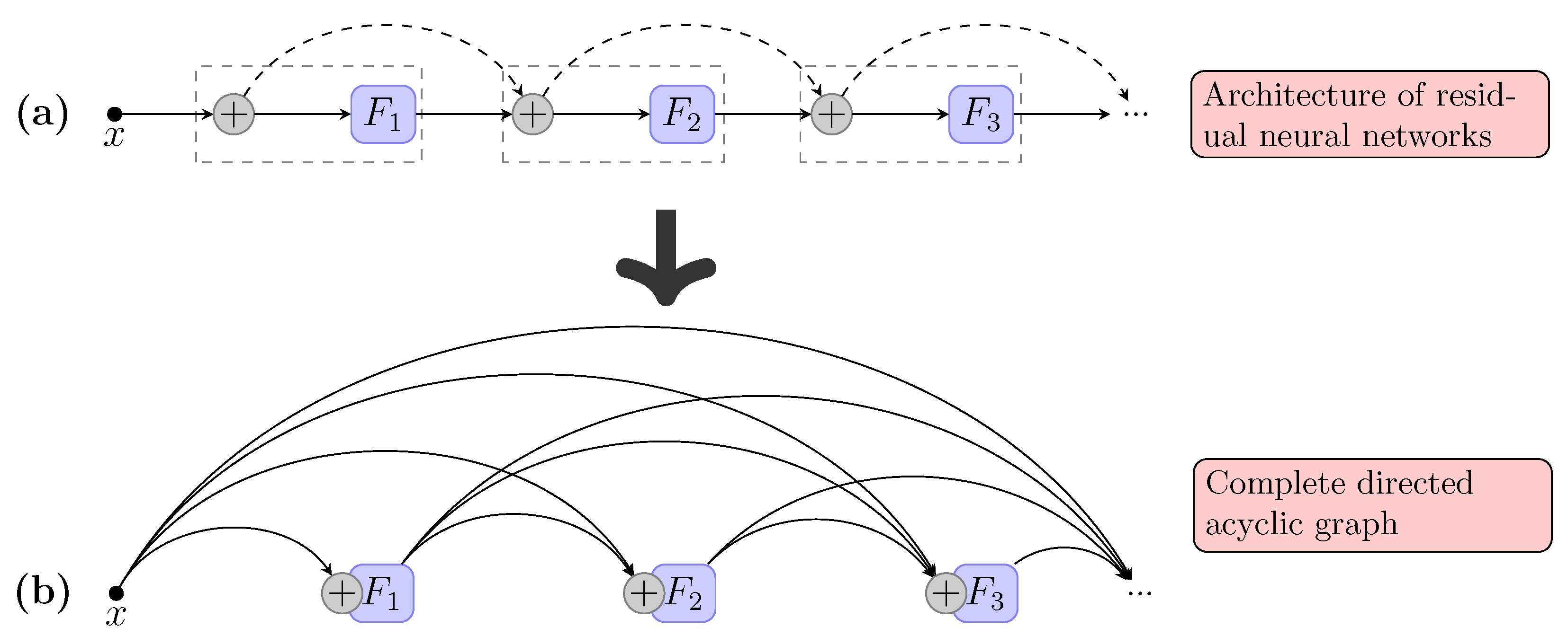
Consider a batch of images which is passed through a residual convolutional neural network. The network comprises L layers, each of which implements a non-linear transformation , where indexes the layer. can be a composite function of operations such as batch normalization (BN), rectified linear units (ReLU), pooling, or convolution (Conv) [34,35]. Residual neural networks [2,3] have a skip connection for every layer that bypasses the non-linear transformations with an identity function. Figure 1a outlines the network structure, where all the dashed lines representing skip connections form the direct path. The skip connections in residual neural networks allow the forward activations and the backward gradients to flow directly through the identity function without information loss, which is the origin of their high performance.
3.2. Improving the Incoherence of DAGs by Folding Residual Neural Networks
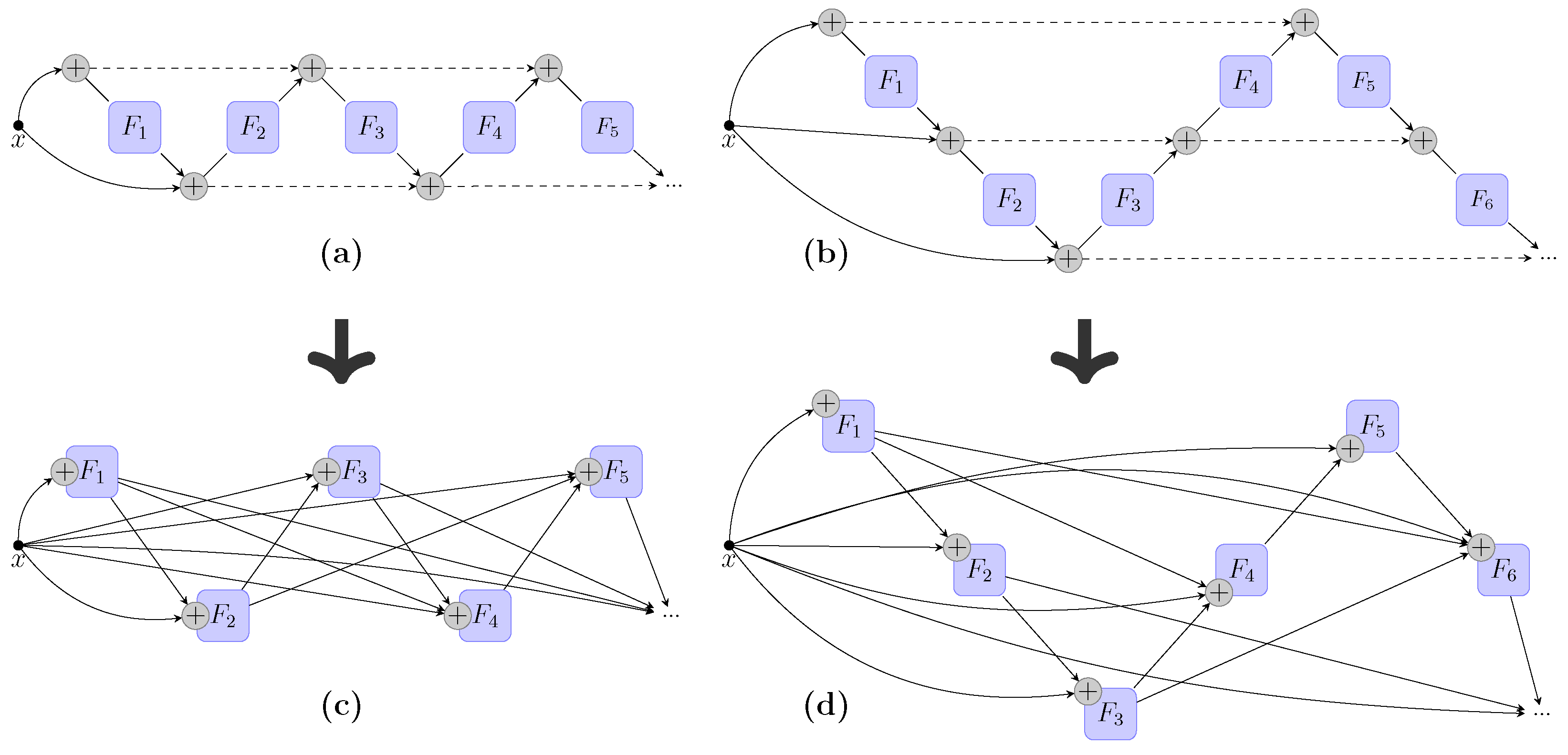
We observed that all the skip connections in residual neural networks only connect adjacent layers, i.e., folding length, besides the width and depth. The distances between any two layers connected by skip connections always equal one, which may restrict its represented capability. Thus, we fold the backbone chain of residual neural networks back and forth to form an accordion-like architecture, as shown in Figure 2a,b.
Such an accordion-like structure extends the chain-like structure of residual neural networks from two aspects. First, the number of direct paths increases from one to multiple, while the particular number of direct paths is determined by the so-called “folding length”. Second, the distances between layers connected by skip connections are different from each other, while the particular values of distances are also determined by the so-called “folding length”. For example, in Figure 2b, where the “folding length” is equal to 3, there are 3 direct paths and the distances between layers connected by skip connections are equal to 2 or 4. Thus, we incorporated a new control parameter d to represent the folding length. For convenience, we named such a folded neural network FoldNet-d, where d is the folding length. In FoldNet-d, the number of direct paths is equal to d and the distances of skip connections are integers in the set . When , the model degenerated to the traditional residual neural networks. Figure 1a and Figure 2a,b illustrate the architectures of FoldNet-1, FoldNet-2, and FoldNet-3, respectively.
According to the mapping rule of the previous subsection, FoldNet-2 and FoldNet-3 could be mapped to DAGs, as shown in (Figure 2). We next explore the incoherence and path lengths of DAGs. As shown in the main plot in Figure 3, we found that the incoherence parameter q increases with the number of nodes in DAGs, which equal the number of layers (or depth) of the corresponding neural networks. We also find that the incoherence parameter q increases with the folding length d. The inset plot in Figure 3 shows the cumulative distribution function (CDF) of path lengths in DAGs when the number of nodes is equal to 50. The inset plot indicates that the proportion of shorter paths increases with the folding length d.
The comparison of incoherence and path lengths between FoldNet-d, where and traditional residual neural networks where show that FoldNet-d has a higher degree of disorder and a larger proportion of shorter paths, and we argue that these two features together lead to the better performance of FoldNet-d.
3.3. Architecture Design
FoldNet model can be formally expressed by the following equation:
where the output of the current layer , , equal to the summation of the non-linear transformation of the output of the previous layer and the output of a previous layer , is . i is the distance between the current layer l and a previous layer which is connected to the current layer by a skip connection. The distance i is determined by the current layer index l and the folding length d. It should be noted that if then , where FoldNet is exactly the same as the traditional residual neural networks. For the case of the folding length , if the current layer index is less than the folding length, , then the previous layer is always equal to . Otherwise, the distance i is determined by:
The distances of skip connections i are constant and always equal to one in traditional residual networks, while in FoldNet they are variable values determined by the current layer index l and the folding length d using Equation (3). The variable distances allow the model to merge and fuse a larger number of previous images which have receptive fields of different sizes, and, thus, enhance its multi-scale representation ability.
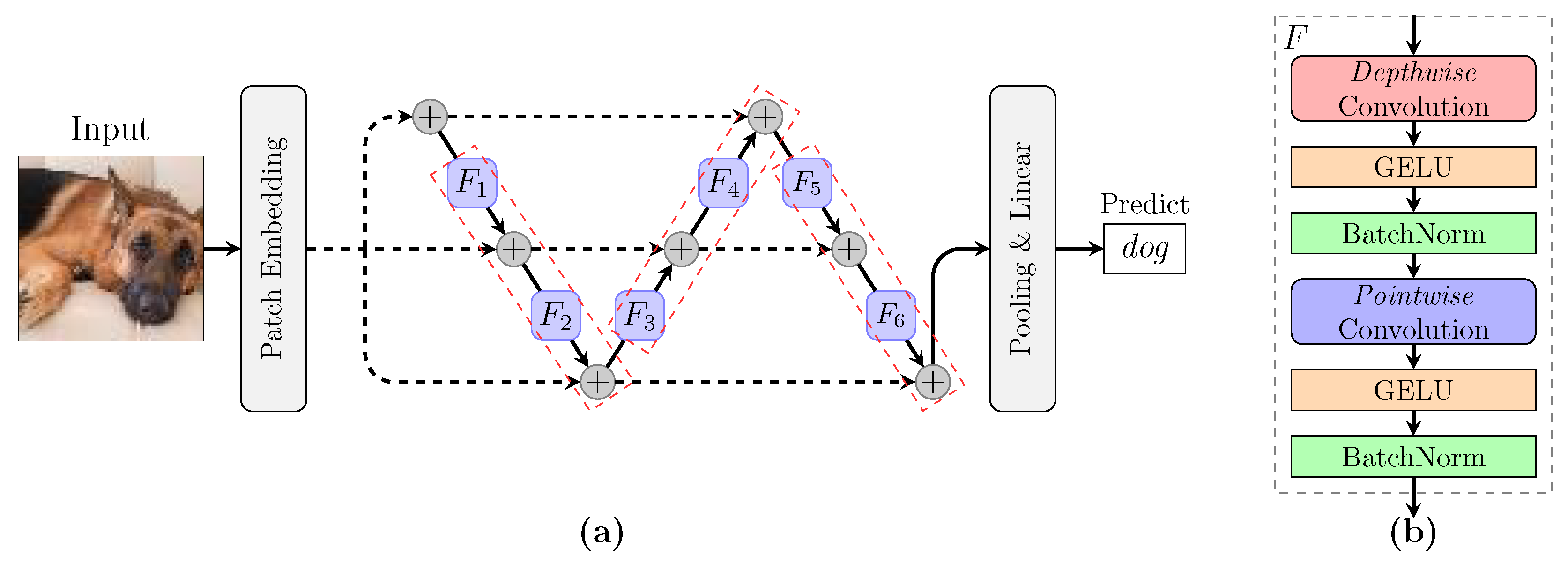
As illustrated in Figure 4a, FoldNet consists of a patch embedding layer followed by repeated applications of a folding block. After many applications of this block, we performed global average pooling to obtain a feature vector, which was then passed to a linear classifier and a softmax function to predict the probabilities of all classes.
The patch embedding layer with patch size p and hidden dimension h can be implemented as convolution with input channels (equal to 3 for RGB images), h output channels, kernel size p and stride p.
The folding block includes non-linear transformations , as shown in the red-dashed rectangles in Figure 4a. Each non-linear transformation itself consists of a depthwise convolution followed by pointwise convolution, and each of the convolutions is followed by an activation GELU and post-activation BatchNorm, as illustrated in Figure 4b. The depthwise convolution is a grouped convolution with a kernel size and groups equal to the number of channels h; the pointwise convolution is a convolution with a kernel size 1 × 1.
Therefore, the architecture of FoldNet is mainly determined by five hyper-parameters: (1) the “width” or hidden dimension h, (2) the depth n or the number of repetitions of non-linear transformation F, (3) the folding length d or the number of non-linear transformations per block, (4) the patch size p which controls the internal resolution of the model, and (5) the kernel size k of the depthwise convolution.
4. Experiments
4.1. Experimental Setup
For image classification, we used the CIFAR-10 and Tiny ImageNet datasets for training. The CIFAR-10 dataset consists of colored natural images with 32 × 32 pixels drawn from 10 classes. The training and test sets contain 50,000 and 10,000 images, respectively. The Tiny ImageNet dataset is a modified subset of the original ImageNet dataset. It consists of colored natural images with pixels drawn from 200 different classes instead of 1000 classes in the ImageNet dataset. The training and test sets contain 100,000 examples and 10,000 examples, respectively.
We implemented FoldNet using the Pytorch framework, and evaluated it using the Pytorch Lightning library. We used the free online P100 GPU provided by Kaggle Kernels to train and evaluate our models on image classification. Kaggle Kernels implement a limit on each user’s GPU use of 30 h/week and 10 h/session. We also used the free and paid online GPUs provided by paperspace.com when the free GPU of Kaggle Kernels could not fulfill our requirements for GPUs.
Due to our limited computing power, we only considered hyperparameters that are critical for the performance of FoldNet, and kept all other hyperparameters constant. FoldNet only changes the method for connecting skip connections among the layers in residual neural networks, and is a macro design methodology for neural-network architectures. Thus, we focused on the depth n and the folding length d, which reflect the macro design of FoldNet, while keeping the hidden dimension h, the patch size p and the kernel size k, which reflect the micro design in the layer level of FoldNet, to their optimized values. We set the patch size and the kernel size , as suggested in the related isotropic model, ConvMixer [25].
For the CIFAR-10 dataset, we trained FoldNet for 100 epochs with a batch size of 256. For the Tiny ImageNet dataset, due to our limited computation power, we trained FoldNet for 50 epochs with a batch size of 128. For both CIFAR-10 and Tiny ImageNet, we used AdamW [36] with a learning rate of and a weight decay of 0.1. There is a 10-epoch linear warmup with an initial learning rate of and a cosine decaying schedule afterward. For data augmentation, we included RandomHorizontalFlip and RandAugment [37].
4.2. Experimental Results of CIFAR-10
To show that the effect of the depth n and the folding length d of FoldNet on its performance is orthogonal to other hyperparameters such as hidden dimension h, we show experimental results for both and .
For each hidden dimension , to evaluate the effect of the depth n and the folding length d of FoldNet on its performance during image classification, we evaluated the depths in a sequence , and for each depth n, we evaluated the folding length in a sequence . There are, in total, 24 evaluations as listed in Table 1. We conducted each evaluation three times, and reported the mean value of the maximum validation accuracy of three runnings as the performance measurement.
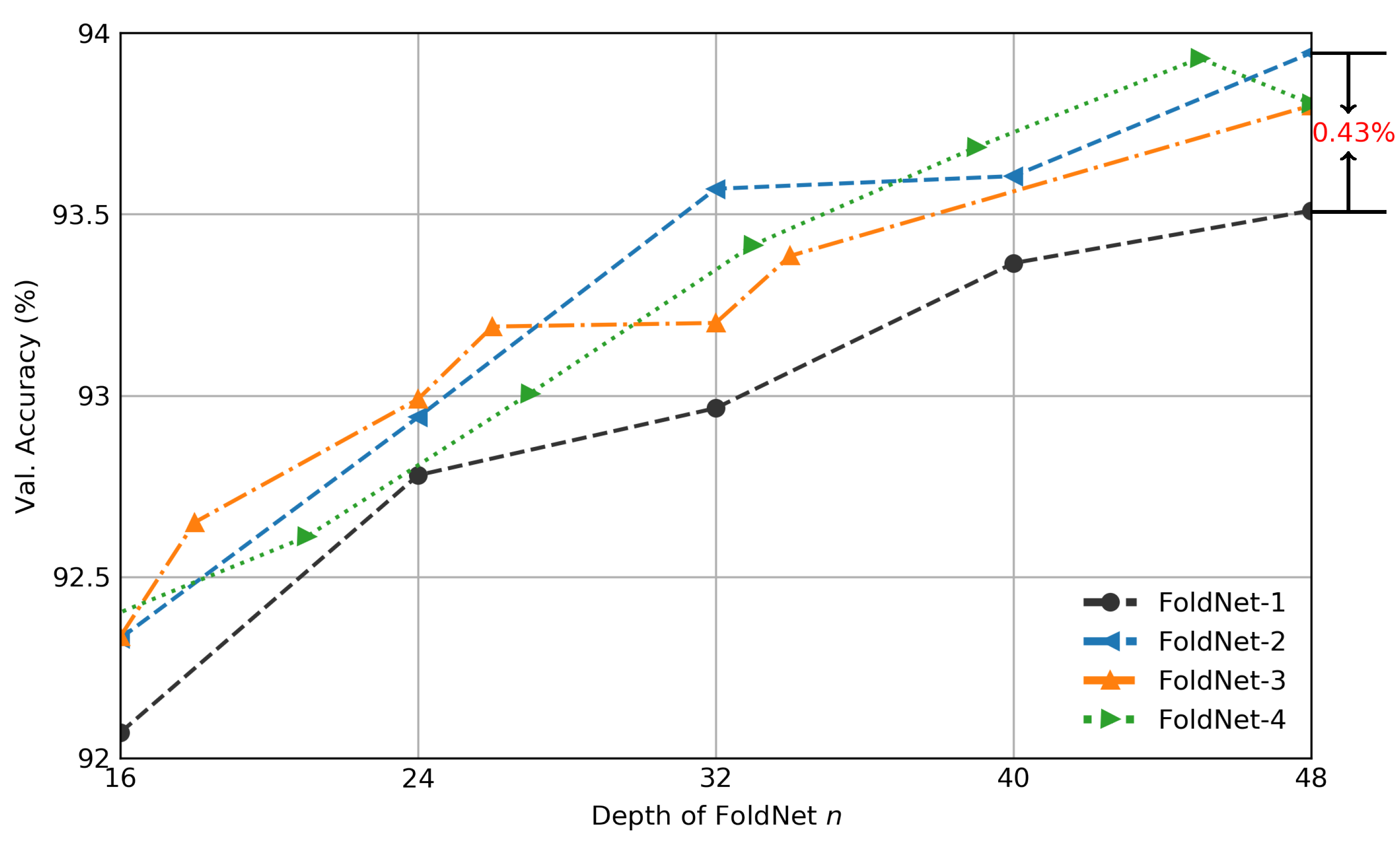
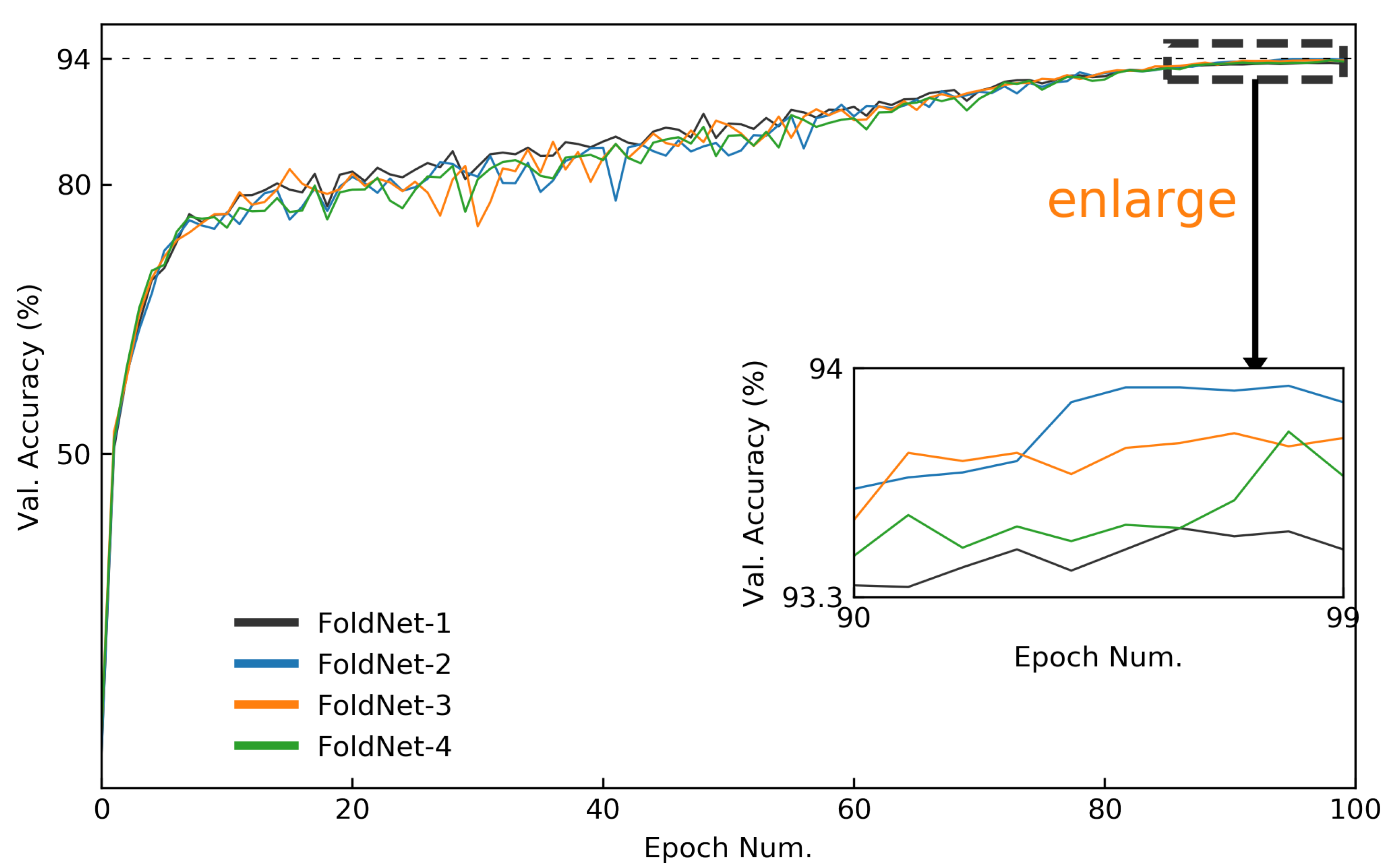
Figure 5 depicts the validation accuracy of FoldNet-1, FoldNet-2, FoldNet-3 and FoldNet-4 when hidden dimension . As shown in the figure, the performance of all the FoldNet models increases with the depth n of FoldNet, and FoldNet-2, FoldNet-3 and FoldNet-4 where perform better than FoldNet-1, where at all the depths. As we show in Figure 3, the incoherence of DAGs is strongly positively correlated with the depth n and folding length d of the corresponding neural networks; thus, we could infer a strong positive correlation between the incoherence of DAGs and the classification accuracy of the corresponding neural networks. In particular, FoldNet-2 with depth has 0.293M parameters and can achieve 93.95% top-1 accuracy on CIFAR-10 after 100 epochs, which increases by 0.43% compared with FoldNet-1 with depth . We also show the validation accuracy curves of FoldNet-1, FoldNet-2, FoldNet-3 and FoldNet-4, when depth , in Figure 6, to compare their performances in detail.
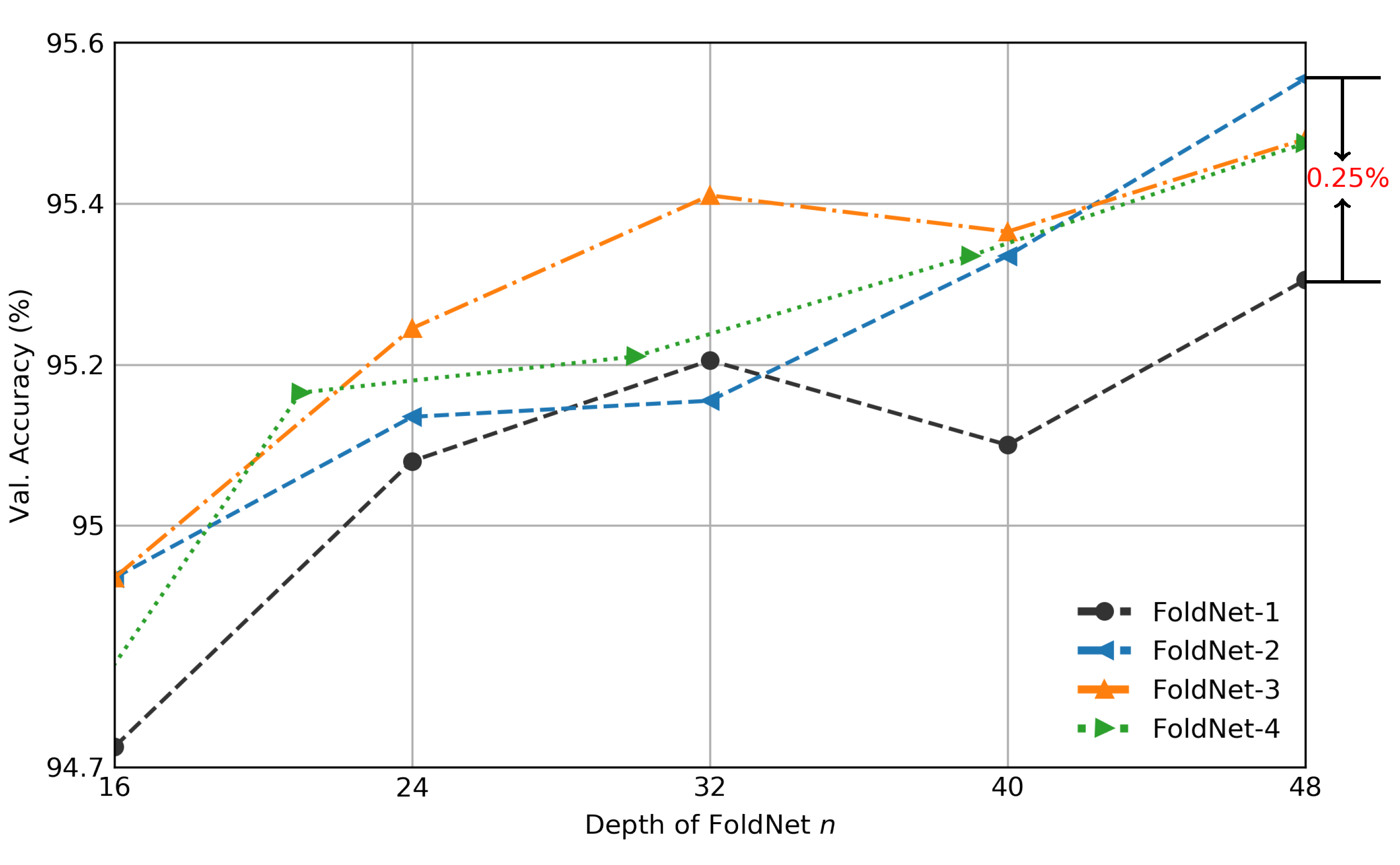
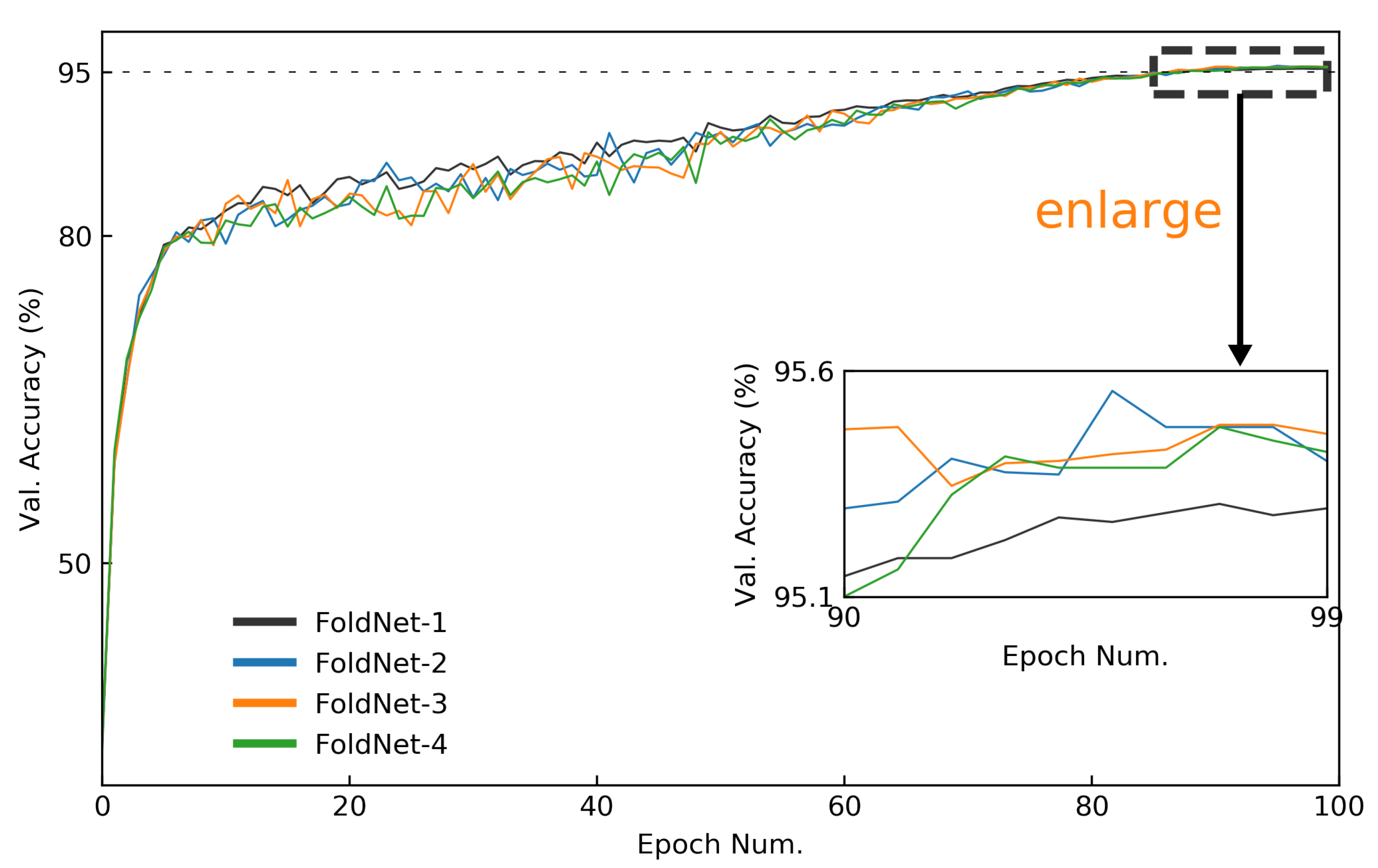
We also show the validation accuracy of FoldNet-1, FoldNet-2, FoldNet-3 and FoldNet-4 when the hidden dimension , in Figure 7. Similar to the case of in Figure 5, the performances of all the FoldNet models increase with the depth n of FoldNet, and FoldNet-2, FoldNet-3 and FoldNet-4, where models with perform better than FoldNet-1, where at almost all depths. In particular, FoldNet-2 with a depth has 3.5M parameters and can achieve 95.56% top-1 accuracy on CIFAR-10 after 100 epochs, which is an increase by 0.25% compared with FoldNet-1 with depth . We also show the validation-accuracy curves of FoldNet-1, FoldNet-2, FoldNet-3 and FoldNet-4 when depth in Figure 8 to compare their performances in detail.
4.3. Experimental Results of Tiny ImageNet
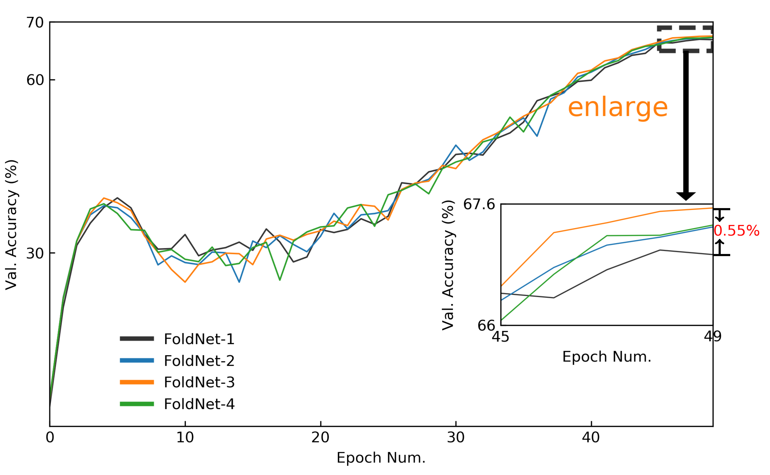
We first evaluated the performances of FoldNet-1, FoldNet-2, FoldNet-3 and FoldNet-4 when hidden dimension and network depth . As shown in Figure 9, FoldNet-3 has 2.4M parameters and can achieve 67.55% top-1 accuracy on Tiny ImageNet after only 50 epochs, which is an increase by 0.55% compared with FoldNet-1.
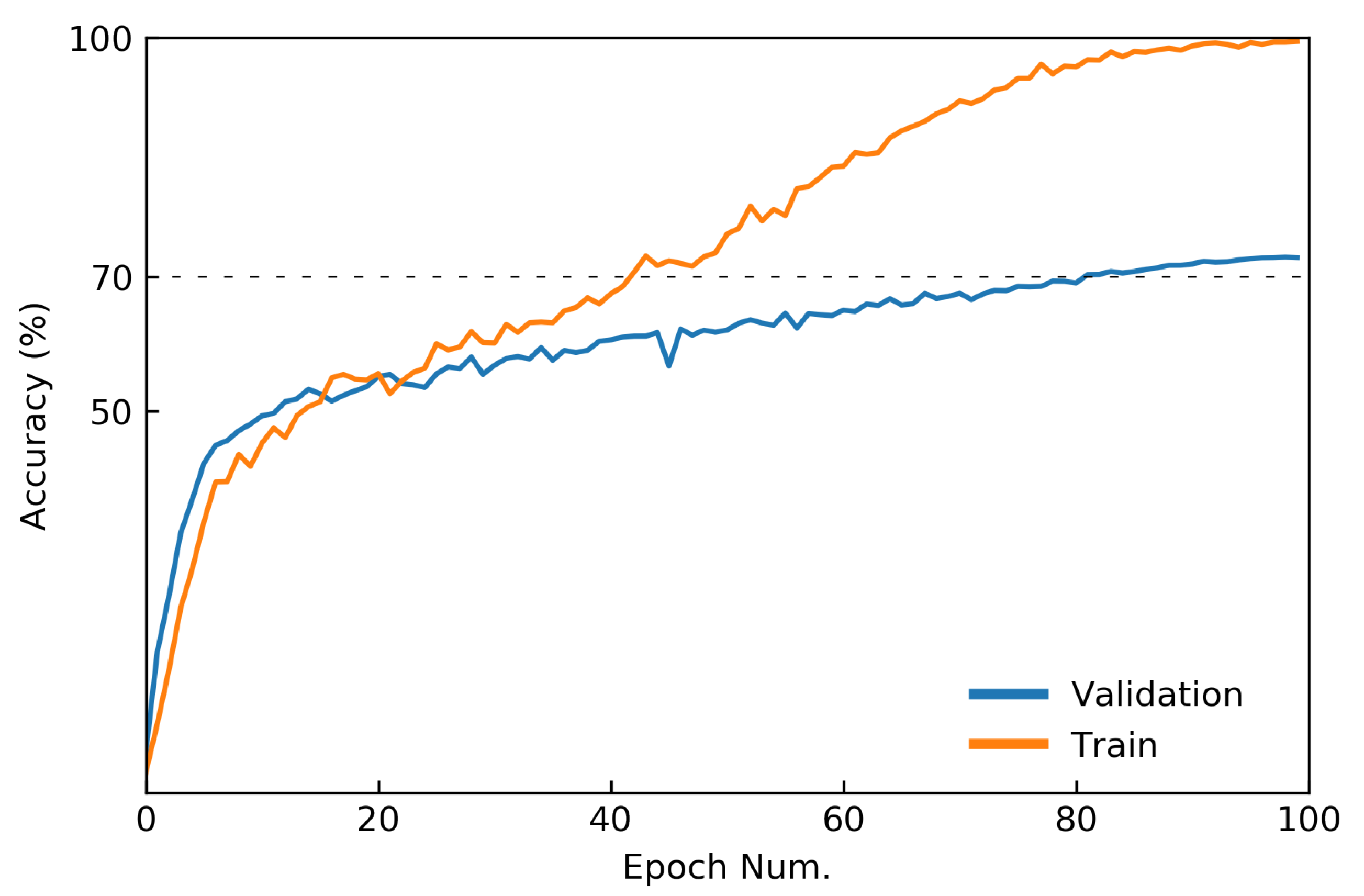
The state-of-the-art model on the Tiny ImageNet dataset, AutoMix [38], achieved 70.24% top-1 accuracy on Tiny ImageNet by adding data-augmentation techniques to the ResNext50_32×4 model [17]. To compare with AutoMix, we added the Mixup [39] data-augmentation technique for FoldNet. We also increased the hidden dimension to and the depth to , and such a FoldNet model has 25.4M parameters that nearly equal the parameters of the ResNext50_32×4 model. We trained the FoldNet model for 100 epochs rather than 50 epochs.
Table 2 shows results on the top-1 accuracies of image classification. For the case of models without Mixup, when compared with the ResNext50_32×4, all the FoldNet models improve the classification performance of Tiny ImageNet by more than 2.44%, which indicates the good performance of the deep-isotropic architecture backbone of FoldNet. When compared among the FoldNet models, the best model, FoldNet-3, performs better than the FoldNet-1 model by 0.58%. For the case of models with Mixup, when compared with the ResNext50_32×4 with Mixup, i.e., AutoMix, all the FoldNet models improve the accuracy by more than 1.77%. When compared among the FoldNet models, the best model, FoldNet-4, performs better than the FoldNet-1 model by 0.63%. We shows the accuracy curves of the best model, FoldNet-4 with Mixup, in Figure 10.
5. Discussion
In this paper, we attempt to apply the insights from the field of complex networks to the structural features of a network affecting its dynamics with regard to deep neural networks. To this end, we mapped the architectures of deep neural networks to DAGs, and then determined the relationship between the structural characteristics of neural networks and corresponding DAGs. We found a strong positive corelation between the incoherence of DAGs and the depth n and folding length d of corresponding neural netowrks. Thus, we propose a deep-isotropic neural-network architecture, FoldNet, by folding a chain of the same blocks whose corresponding DAGs are more incoherent.
We evaluated the effect of FoldNet on image classification by varying their depth n and folding length d. We found a positive correlation between the depth and folding length of FoldNet and their accuracy. Therefore, we inferred that the incoherence of DAGs has a positive relationship with the accuracy of the corresponding neural networks in image classification. FoldNet achieved competitive results on the Tiny ImageNet dataset with far fewer parameters.
We recognize that the performance of a neural network may be affected by multiple structural features at the same time, rather than one—for example, the incoherence in our case. DAGs have other structural features, such as the number of paths in DAG, which can affect the performances of corresponding neural networks. In addition, we only explored FoldNet-d with , as we did not find notable performance increments when . This is also a clue that structural features other than the incoherence may affect the performance of a neural network. Our future work will explore this direction.
Author Contributions
Conceptualization, W.F. and X.Z.; methodology, X.Z. and W.F.; software, W.F.; validation, Q.S. and G.S.; formal analysis, W.F.; investigation, W.F.; resources, Q.S. and G.S.; data curation, Q.S. and G.S.; writing—original draft preparation, W.F. and X.Z.; writing—review and editing, X.Z.; visualization, Q.S. and G.S.; supervision, W.F.; project administration, W.F.; funding acquisition, W.F. All authors have read and agreed to the published version of the manuscript.
Funding
This research was funded by the Program of New Century Excellent Talents in University of China (no. NCET-11-0942) and the Program of National Natural Science Foundation of China (no. 60703053).
Data Availability Statement
The CIFAR-10 dataset refered to in this study are openly available in “Learning multiple layers of features from tiny images” at https://www.cs.toronto.edu/~kriz/cifar.html, accessed on 9 April 2022; the Tiny ImageNet dataset refered to in this study are openly available at https://www.kaggle.com/c/tiny-imagenet, accessed on 9 April 2022. The code is publicly available at https://github.com/keepsimpler/sunyata, accessed on 10 August 2022.
Acknowledgments
We gratefully acknowledge the P100 GPU support provided by kaggle.com and the A4000, A5000 GPU support provided by paperspace.com.
Conflicts of Interest
The authors declare no conflict of interest.
Abbreviations
The following abbreviations are used in this manuscript:
| DAG | directed acyclic graphs |
| trophic level of node i in DAG | |
| A | adjacency matrix of DAG |
| in degrees of node i in DAG | |
| out degrees of node i in DAG | |
| q | incoherence parameter of DAG |
| output of layer l in FoldNet | |
| non-linear transformations of layer l in FoldNet | |
| d | folding length of FoldNet |
| h | hidden dimension of FoldNet |
| n | number of non-linear transformations F in FoldNet |
| p | patch size |
| k | kernel size of depthwise convolution |
| CNN | convolutional neural network |
| MLP | multiple layer network |
References
- Caudill, M. Neural Networks Primer, Part I. AI Expert 1987, 2, 46–52. [Google Scholar]
- He, K.; Zhang, X.; Ren, S.; Sun, J. Deep residual learning for image recognition. In Proceedings of the IEEE Conference on Computer Vision and Pattern Rrecognition, Las Vegas, NV, USA, 27–30 June 2016; pp. 770–778. [Google Scholar]
- He, K.; Zhang, X.; Ren, S.; Sun, J. Identity mappings in deep residual networks. In Proceedings of the European Conference on Computer Vision, Amsterdam, The Netherlands, 11–14 October 2016; Springer: Berlin/Heidelberg, Germany, 2016; pp. 630–645. [Google Scholar]
- Huang, G.; Liu, Z.; Van Der Maaten, L.; Weinberger, K.Q. Densely connected convolutional networks. In Proceedings of the IEEE Conference on Computer Vision and Pattern Recognition, Honolulu, HI, USA, 21–26 July 2017; pp. 4700–4708. [Google Scholar]
- Li, L.; Talwalkar, A. Random search and reproducibility for neural architecture search. In Proceedings of the Uncertainty in Artificial Intelligence, PMLR, Online Conference, 3–6 August 2020; pp. 367–377. [Google Scholar]
- Pham, H.; Guan, M.; Zoph, B.; Le, Q.; Dean, J. Efficient neural architecture search via parameters sharing. In Proceedings of the International Conference on Machine Learning, PMLR, Baltimore, MD, USA, 17–23 July 2018; pp. 4095–4104. [Google Scholar]
- Yu, K.; Sciuto, C.; Jaggi, M.; Musat, C.; Salzmann, M. Evaluating The Search Phase of Neural Architecture Search. In Proceedings of the 8th International Conference on Learning Representations, ICLR, Addis Ababa, Ethiopia, 26–30 April 2020. [Google Scholar]
- Zoph, B.; Vasudevan, V.; Shlens, J.; Le, Q.V. Learning transferable architectures for scalable image recognition. In Proceedings of the IEEE Conference on Computer Vision and Pattern Recognition, Salt Lake City, UT, USA, 18–23 June 2018; pp. 8697–8710. [Google Scholar]
- Newman, M. Networks: An Introduction; Oxford University Press, Inc.: New York, NY, USA, 2010. [Google Scholar]
- Testolin, A.; Piccolini, M.; Suweis, S. Deep learning systems as complex networks. J. Complex Netw. 2020, 8, cnz018. [Google Scholar] [CrossRef]
- Xie, S.; Kirillov, A.; Girshick, R.; He, K. Exploring randomly wired neural networks for image recognition. In Proceedings of the IEEE/CVF International Conference on Computer Vision, Seoul, Korea, 27 October–2 November 2019; pp. 1284–1293. [Google Scholar]
- Erdos, P.; Rényi, A. On the evolution of random graphs. Publ. Math. Inst. Hung. Acad. Sci 1960, 5, 17–60. [Google Scholar]
- Albert, R.; Barabási, A.L. Statistical mechanics of complex networks. Rev. Mod. Phys. 2002, 74, 47. [Google Scholar] [CrossRef] [Green Version]
- Watts, D.J.; Strogatz, S.H. Collective dynamics of ‘small-world’networks. Nature 1998, 393, 440–442. [Google Scholar] [CrossRef]
- Simonyan, K.; Zisserman, A. Very Deep Convolutional Networks for Large-Scale Image Recognition. In Proceedings of the 3rd International Conference on Learning Representations, ICLR, San Diego, CA, USA, 7–9 May 2015. [Google Scholar]
- Zagoruyko, S.; Komodakis, N. Wide Residual Networks. In Proceedings of the British Machine Vision Conference 2016, York, UK, 19–22 September 2016. [Google Scholar]
- Xie, S.; Girshick, R.; Dollár, P.; Tu, Z.; He, K. Aggregated residual transformations for deep neural networks. In Proceedings of the IEEE Conference on Computer Vision and Pattern Recognition, Honolulu, HI, USA, 21–26 July 2017; pp. 1492–1500. [Google Scholar]
- Chollet, F. Xception: Deep learning with depthwise separable convolutions. In Proceedings of the IEEE Conference on Computer Vision and Pattern Recognition, Honolulu, HI, USA, 21–26 July 2017; pp. 1251–1258. [Google Scholar]
- Tan, M.; Le, Q. Efficientnet: Rethinking model scaling for convolutional neural networks. In Proceedings of the International Conference on Machine Learning, PMLR, Long Beach, CA, USA, 9–15 June 2019; pp. 6105–6114. [Google Scholar]
- Sandler, M.; Howard, A.; Zhu, M.; Zhmoginov, A.; Chen, L.C. Mobilenetv2: Inverted residuals and linear bottlenecks. In Proceedings of the IEEE Conference on Computer Vision and Pattern Recognition, Salt Lake City, UT, USA, 18–23 June 2018; pp. 4510–4520. [Google Scholar]
- Szegedy, C.; Ioffe, S.; Vanhoucke, V.; Alemi, A.A. Inception-v4, inception-resnet and the impact of residual connections on learning. In Proceedings of the Thirty-first AAAI Conference on Artificial Intelligence, San Francisco, CA, USA, 4–9 February 2017. [Google Scholar]
- Vaswani, A.; Shazeer, N.; Parmar, N.; Uszkoreit, J.; Jones, L.; Gomez, A.N.; Kaiser, Ł.; Polosukhin, I. Attention is all you need. Adv. Neural Inf. Process. Syst. 2017, 30, 5998–6008. [Google Scholar]
- Dosovitskiy, A.; Beyer, L.; Kolesnikov, A.; Weissenborn, D.; Zhai, X.; Unterthiner, T.; Dehghani, M.; Minderer, M.; Heigold, G.; Gelly, S.; et al. An Image is Worth 16 × 16 Words: Transformers for Image Recognition at Scale. In Proceedings of the 9th International Conference on Learning Representations, ICLR, Online Conference, Austria, 3–7 May 2021. [Google Scholar]
- Sandler, M.; Baccash, J.; Zhmoginov, A.; Howard, A. Non-discriminative data or weak model? On the relative importance of data and model resolution. In Proceedings of the IEEE/CVF International Conference on Computer Vision Workshops, Seoul, Korea, 27–28 October 2019. [Google Scholar]
- Trockman, A.; Kolter, J.Z. Patches are all you need? arXiv 2022, arXiv:2201.09792. [Google Scholar]
- Tolstikhin, I.O.; Houlsby, N.; Kolesnikov, A.; Beyer, L.; Zhai, X.; Unterthiner, T.; Yung, J.; Steiner, A.; Keysers, D.; Uszkoreit, J.; et al. Mlp-mixer: An all-mlp architecture for vision. Adv. Neural Inf. Process. Syst. 2021, 34, 24261–24272. [Google Scholar]
- Touvron, H.; Bojanowski, P.; Caron, M.; Cord, M.; El-Nouby, A.; Grave, E.; Izacard, G.; Joulin, A.; Synnaeve, G.; Verbeek, J.; et al. Resmlp: Feedforward networks for image classification with data-efficient training. IEEE Trans. Pattern Anal. Mach. Intell. 2022; in press. [Google Scholar]
- Karrer, B.; Newman, M.E. Random graph models for directed acyclic networks. Phys. Rev. E 2009, 80, 046110. [Google Scholar] [CrossRef] [PubMed] [Green Version]
- Johnson, S.; Domínguez-García, V.; Donetti, L.; Munoz, M.A. Trophic coherence determines food-web stability. Proc. Natl. Acad. Sci. USA 2014, 111, 17923–17928. [Google Scholar] [CrossRef] [Green Version]
- Domínguez-García, V.; Johnson, S.; Muñoz, M.A. Intervality and coherence in complex networks. Chaos Interdiscip. J. Nonlinear Sci. 2016, 26, 065308. [Google Scholar] [CrossRef] [PubMed]
- Klaise, J.; Johnson, S. From neurons to epidemics: How trophic coherence affects spreading processes. Chaos Interdiscip. J. Nonlinear Sci. 2016, 26, 065310. [Google Scholar] [CrossRef] [PubMed] [Green Version]
- MacKay, R.S.; Johnson, S.; Sansom, B. How directed is a directed network? R. Soc. Open Sci. 2020, 7, 201138. [Google Scholar] [CrossRef] [PubMed]
- Veit, A.; Wilber, M.J.; Belongie, S. Residual networks behave like ensembles of relatively shallow networks. Adv. Neural Inf. Process. Syst. 2016, 29, 550–558. [Google Scholar]
- Ioffe, S.; Szegedy, C. Batch normalization: Accelerating deep network training by reducing internal covariate shift. In Proceedings of the International Conference on Machine Learning, PMLR, Lille, France, 6–11 July 2015; pp. 448–456. [Google Scholar]
- LeCun, Y.; Bottou, L.; Bengio, Y.; Haffner, P. Gradient-based learning applied to document recognition. Proc. IEEE 1998, 86, 2278–2324. [Google Scholar] [CrossRef]
- Loshchilov, I.; Hutter, F. Decoupled Weight Decay Regularization. In Proceedings of the 7th International Conference on Learning Representations, ICLR, New Orleans, LA, USA, 6–9 May 2019. [Google Scholar]
- Cubuk, E.D.; Zoph, B.; Shlens, J.; Le, Q.V. Randaugment: Practical automated data augmentation with a reduced search space. In Proceedings of the IEEE/CVF Conference on Computer Vision and Pattern Recognition Workshops, Glasgow, UK, 23–28 August 2020; pp. 702–703. [Google Scholar]
- Ramé, A.; Sun, R.; Cord, M. Mixmo: Mixing multiple inputs for multiple outputs via deep subnetworks. In Proceedings of the IEEE/CVF International Conference on Computer Vision, New Orleans, LA, USA, 11–17 October 2021; pp. 823–833. [Google Scholar]
- Zhang, H.; Cisse, M.; Dauphin, Y.N.; Lopez-Paz, D. mixup: Beyond empirical risk minimization. arXiv 2017, arXiv:1710.09412. [Google Scholar]
Figure 1.
Example of mapping from residual neural networks to directed acyclic graphs (DAGs). (a) An example of the architecture of residual neural networks. The nodes represent non-linear transformations among data; the circles with plus signs inside represent summation of all ingoing data. (b) The complete directed acyclic graph mapped from the residual neural network. The nodes are compositions of summation and non-linear transformations; the lines represent data flows among nodes.

Figure 2.
Example of mapping from FoldNet to DAGs. (a) An example of FoldNet-2. (b) An example of FoldNet-3. The nodes represent non-linear transformations among data; the circles with plus signs inside represent summation of all ingoing data. (c) The directed acyclic graph mapped from FoldNet-2. (d) The directed acyclic graph mapped from FoldNet-3. The nodes are composition of summation and non-linear transformations; the lines represent data flows among nodes.

Figure 3.
Incoherence and path lengths of DAGs. The main plot illustrates the relationship between incoherence parameter q and number of nodes of DAGs and folding length d. The inset plot shows the relationship between path lengths and folding length d.
Figure 3.
Incoherence and path lengths of DAGs. The main plot illustrates the relationship between incoherence parameter q and number of nodes of DAGs and folding length d. The inset plot shows the relationship between path lengths and folding length d.

Figure 4.
(a) Architecture of the FoldNet model. FoldNet starts with the patch embedding layer, continues with multiple folding blocks shown by the red-dashed rectangles, followed by the pooling and the linear softmax classifier. Here, the depth , the folding length , and the number of folding blocks equals . (b) Details of each non-linear transformation , including a depthwise convolution followed by an GELU activation and a post-activation BatchNorm. After that followed a pointwise convolution, another GELU activation, and another post-activation BatchNorm.

Figure 5.
Validation accuracy of FoldNet-d for CIFAR-10 dataset when hidden dimension . x axis is the depth of neural network n; y axis is the validation accuracy percentage. The validation accuracy of FoldNet-2 increases by compared with FoldNet-1 when depth .
Figure 5.
Validation accuracy of FoldNet-d for CIFAR-10 dataset when hidden dimension . x axis is the depth of neural network n; y axis is the validation accuracy percentage. The validation accuracy of FoldNet-2 increases by compared with FoldNet-1 when depth .

Figure 6.
Validation accuracy curves of FoldNet for CIFAR-10 dataset when hidden dimension and network depth . The validation accuracy curves of the last 10 epochs are enlarged to compare the accuracies of FoldNet-d more clearly.
Figure 6.
Validation accuracy curves of FoldNet for CIFAR-10 dataset when hidden dimension and network depth . The validation accuracy curves of the last 10 epochs are enlarged to compare the accuracies of FoldNet-d more clearly.

Figure 7.
Validation accuracy of FoldNet-d for CIFAR-10 dataset when hidden dimension . x axis is the depth of neural network n, y axis is the validation accuracy percentage. The validation accuracy of FoldNet-2 increases by compared with FoldNet-1 when depth .
Figure 7.
Validation accuracy of FoldNet-d for CIFAR-10 dataset when hidden dimension . x axis is the depth of neural network n, y axis is the validation accuracy percentage. The validation accuracy of FoldNet-2 increases by compared with FoldNet-1 when depth .

Figure 8.
Validation-accuracy curves of FoldNet for CIFAR-10 dataset when hidden dimension and network depth . The validation accuracy curves of the last 10 epochs are enlarged to compare the accuracies of FoldNet-d more clearly.
Figure 8.
Validation-accuracy curves of FoldNet for CIFAR-10 dataset when hidden dimension and network depth . The validation accuracy curves of the last 10 epochs are enlarged to compare the accuracies of FoldNet-d more clearly.

Figure 9.
Validation-accuracy curves of FoldNet for Tiny ImageNet dataset when hidden dimension and network depth . The validation-accuracy curves of the last five epochs are enlarged to compare the accuracies of FoldNet-d more clearly.
Figure 9.
Validation-accuracy curves of FoldNet for Tiny ImageNet dataset when hidden dimension and network depth . The validation-accuracy curves of the last five epochs are enlarged to compare the accuracies of FoldNet-d more clearly.

Figure 10.
Accuracy curves of FoldNet-4 with Mixup on the Tiny ImageNet dataset when hidden dimension and network depth .
Figure 10.
Accuracy curves of FoldNet-4 with Mixup on the Tiny ImageNet dataset when hidden dimension and network depth .


Table 1.
Hyperparameter values for CIFAR-10 dataset. The depth n is equal to the number of folding blocks times . The patch size p and kernel size k are fixed as and . The hidden dimension h was chosen from the set [64, 256].
Table 1.
Hyperparameter values for CIFAR-10 dataset. The depth n is equal to the number of folding blocks times . The patch size p and kernel size k are fixed as and . The hidden dimension h was chosen from the set [64, 256].
| Folding Length d | Num. of Folding Blocks | Corresponding Depth n |
|---|---|---|
| 1 | [16, 24, 32, 40, 48] | [16, 24, 32, 40, 48] |
| 2 | [16, 24, 32, 40, 48] | [16, 24, 32, 40, 48] |
| 3 | [8, 9, 12, 13, 16, 17, 24] | [16, 18, 24, 26, 32, 34, 48] |
| 4 | [5, 7, 9, 11, 13, 15, 16] | [15, 21, 27, 33, 39, 45, 48] |
Table 2.
Top-1 Acc (%) of image classification on Tiny ImageNet.
| Models w/o Mixup | Top-1 Acc (%) | Models w/o Mixup | Top-1 Acc (%) |
|---|---|---|---|
| ResNext50_32×4 | 68.45 | AutoMix [38] | 70.24 |
| FoldNet-1 | 70.89 | FoldNet-1 | 72.01 |
| FoldNet-2 | 71.43 | FoldNet-2 | 72.59 |
| FoldNet-3 | 71.49 | FoldNet-3 | 72.64 |
| FoldNet-4 | 71.47 | FoldNet-4 | 72.67 |
Publisher’s Note: MDPI stays neutral with regard to jurisdictional claims in published maps and institutional affiliations. |
© 2022 by the authors. Licensee MDPI, Basel, Switzerland. This article is an open access article distributed under the terms and conditions of the Creative Commons Attribution (CC BY) license (https://creativecommons.org/licenses/by/4.0/).
Share and Cite
MDPI and ACS Style
Feng, W.; Zhang, X.; Song, Q.; Sun, G. The Incoherence of Deep Isotropic Neural Networks Increases Their Performance in Image Classification. Electronics 2022, 11, 3603. https://doi.org/10.3390/electronics11213603
AMA Style
Feng W, Zhang X, Song Q, Sun G. The Incoherence of Deep Isotropic Neural Networks Increases Their Performance in Image Classification. Electronics. 2022; 11(21):3603. https://doi.org/10.3390/electronics11213603
Chicago/Turabian StyleFeng, Wenfeng, Xin Zhang, Qiushuang Song, and Guoying Sun. 2022. "The Incoherence of Deep Isotropic Neural Networks Increases Their Performance in Image Classification" Electronics 11, no. 21: 3603. https://doi.org/10.3390/electronics11213603
Note that from the first issue of 2016, this journal uses article numbers instead of page numbers. See further details here.