Reservoir Prediction Model via the Fusion of Optimized Long Short-Term Memory Network (LSTM) and Bidirectional Random Vector Functional Link (RVFL)

Abstract

An accurate and stable reservoir prediction model is essential for oil location and production. We propose an predictive hybrid model ILSTM-BRVFL based on an improved long short-term memory network (IAOS-LSTM) and a bidirectional random vector functional link (Bidirectional-RVFL) for this problem. Firstly, the Atomic Orbit Search algorithm (AOS) is used to perform collective optimization of the parameters to improve the stability and accuracy of the LSTM model for high-dimensional feature extraction. At the same time, there is still room to improve the optimization capability of the AOS. Therefore, an improvement scheme to further enhance the optimization capability is proposed. Then, the LSTM-extracted high-dimensional features are fed into the random vector functional link (RVFL) to improve the prediction of high-dimensional features by the RVFL, which is modified as the bidirectional RVFL. The proposed ILSTM-BRVFL (IAOS) model achieves an average prediction accuracy of 95.28%, compared to the experimental results. The model’s accuracy, recall values, and F1 values also showed good performance, and the prediction ability achieved the expected results. The comparative analysis and the degree of improvement in the model results show that the high-dimensional extraction of the input data by LSTM is the most significant improvement in prediction accuracy. Secondly, it introduces a double-ended mechanism for IAOS to LSTM and RVFL for parameter search.

1. Introduction

It is well known that oil is a non-renewable energy source. It is the most crucial part of the world’s energy composition. It is used in a vast range of applications. Moreover, improving the accuracy of oil location forecasting directly affects the economics of extraction and use. With decades of technological iterations and upgrades, especially the widespread use of artificial intelligence in recent years, the efficiency of oil location prediction underground has been improving yearly. This is evident from the frequent joint ventures between multinational oil companies and IT companies worldwide in recent years to explore intelligent oil. At present, intelligent exploration and exploitation in the oil and gas industry is a popular direction for some time to come through the in-depth integration of industry, academia, and research. Specifically, in the process of oil exploration and positioning, the logging data from each region is characterized by a large volume of data and multiple sources of heterogeneity. The process of processing log data from exploration is subject to multiple difficulties such as uncertainty. As more and more oil and gas fields are being explored around the world, and new discoveries become more and more difficult to determine, the role of artificial intelligence is becoming more and more apparent. In recent years, it has focused on curve reconstruction [1], reservoir parameter prediction [2], lithology identification [3], imaging log interpretation [4], fracture and fracture hole filling identification [5], and hydrocarbon-bearing properties evaluation [6], physical model simulation calculation [7,8].

As a branch of artificial intelligence, the role of machine learning has become more critical. Especially in recent years, with the increasing maturity of neural network technology, more and more scholars have started to use network models such as feedforward neural networks (BP) [9] and recurrent neural networks (RNN) [10] in artificial neural networks (ANN) to locate and predict oil reservoirs through the oil formation data obtained from exploration. Taha et al. [11] continued on from previous studies in presenting the application of artificial neural network for modeling maximum dry density and optimum water content for soil stabilized with nano-materials. Triveni et al. [12] created two multilayer feedforward neural network (MLFN) models to estimate petrophysical parameters with implications for predicting petroleum reservoirs. Gilani et al. [13] used a back propagation neural network (BPNN) model to predict aquifer sedimentology in logs. Jiang et al. [14] used the boosting tree algorithm to build the Lithology identification model. Zhou et al. [15] established a BiLSTM network model, which can accurately identify different types of strata developed in storage space and significantly improve the accuracy of reservoir identification. Wu et al. [16] developed a code-based convolutional neural network model that enables simultaneous geological fault detection and slope estimation. It significantly outperformed traditional methods in both fault detection and reflection slope calculation. Zhang et al. [17] proposed a method based on the long short-term memory network (LSTM) to reconstruct logging curves, which was validated using natural logging curves and found to be more accurate than the traditional method. Wang et al. [18] used historical data on oilfield production as a benchmark. At the same time, he considered the connection between production indicators and their influencing factors as well as production trends and backward and forward correlations over time, and used the long short-term memory network (LSTM) in the field of deep learning to construct the corresponding oilfield production prediction model to achieve the goal of predicting oilfield production. Zeng et al. [19] designed a bidirectional GRU network to extract key features from forward and backward logging data along the depth direction, and also introduced an attention mechanism to assign different weights to each hidden layer to improve the accuracy of logging prediction and quantitative lithology identification.

In the further field of classification research, Huang et al. [20] proposed a single hidden layer feed-forward neural network (SLFN) called extreme learning machine (ELM), which was shown to have the advantages of high learning efficiency and generalization ability. Duan et al. [21] proposed a hybrid architecture, including convolutional neural network (CNN) and extreme learning machine (ELM) to handle age and Gender classification. The experimental results showed that the hybrid architecture outperformed other studies on the same dataset in terms of accuracy and efficiency. Kumar et al. [22] built a hybrid recurrent neural network and feedforward neural network with RNN-ELM architecture for crime hotspot classification. The learning speed and accuracy were significantly better than RNN. Random vector functional link (RVFL) is also a SLFN network. The main difference between RVFL and ELM is that RVFL includes a direct mapping from input to output. Although the RVFL increases the complexity of the network compared to the ELM, its network parameters are determined in the course of the network. However, it does not require any iterative steps in the determination of the network parameters, which significantly reduces the tuning time of the network parameters. Compared with traditional training methods, this method has the advantages of fast learning speed and good generalization performance [23]. RVFL has been widely used in classification, regression, clustering, feature learning and other problems due to these advantages. Peng et al. [24] developed the JOSRVFL (Joint Optimized Semi-Supervised RVFL) model to compare with JOSELM (Joint Optimized Semi-Supervised ELM) to demonstrate the better performance of the JOSRVFL model in practical applications. Malik et al. [25] proposed a novel ensemble method, known as rotated random vector functional link neural network (RoF-RVFL), which combines rotation forest (RoF) and RVFL classifiers, and the experimental results show that the proposed RoF-Rvfl method can generate a more robust network with better generalization performance. Zhou et al. [26] proposed an improved incremental random vector functional-link network (RVFL) with a compact structure and applies it to the quality prediction of blast furnace (BF) ironmaking processes. Guo et al. [27] proposed a sparse Laplace regularized random vector function link (SLapRVFL) neural network model, which was used for weight assessment of hemodialysis patients to demonstrate higher accuracy than other detection methods. Yu et al. [28] proposed an ensemble learning framework based on the RVFL network model, and used it to perform crude oil price forecasting, where the proposed multistage nonlinear RVFL network ensemble forecasting model was consistently better than that of a single RVFL network model in terms of the same measurements. Aggarwal et al. [29] used the RVFL model to make accurate predictions of solar energy for the previous day and week in Sydney, Australia, in 2015. Chen et al. [30] developed an intelligent system for water quality monitoring based on a fused random vector functional link network (RVFL) and the group method of data processing (GMDH) model. The proposed method had superior performance compared to other state-of-the-art methods. Waheed et al. [31] proposed a Hunger Games Search (HGS) optimizer–optimized random vector function link (RVFL) model, which was used for stir friction welding of heterogeneous polymeric materials to obtain high accuracy rates.

The direct factors affecting the performance of a neural network model are its internal parameters and hyperparameters. Therefore, we can improve its performance by optimizing the network model parameters and hyperparameters. Parameter search through intelligent optimization algorithms are a common optimization method, whereby intelligent optimization algorithms include Genetic Algorithm (GA) [32], Differential Evolution (DE) [33], Ant System (AS) [34], Particle Swarm Algorithm (PSO) [35], etc. The way these intelligent optimization algorithms optimize neural networks is basically by setting the fitness function to find the optimal pairing of the parameters of the neural network in order to achieve the result with the lowest fitness function. In practical applications, Tariq et al. [36] used optimization algorithms such as Differential Evolution (DE), Particle Swarm Optimization (PSO) and Covariance Matrix Adaptive Evolution Strategy (CMAES) to optimize the Functional Network model to build a reservoir water content saturation prediction model using petrophysical logging data as input information. Costa et al. [37] used a combination of neural network model and Genetic Algorithm to predict oilfield production data.

The atomic orbit search algorithm (AOS) [38] used in this study is mainly based on the basic principles of quantum mechanics. It simulates the trajectory of the electron motion around the nucleus, focusing on the feature that the electron can change its motion according to the energy increase or decrease. The proposed algorithm is verified in the literature by comparing the benchmark function with other similar algorithms. In addition, the results prove that the AOS has a good performance and can effectively jump out of local optima to find the global optimum solution.

Inspired by the above literature, this paper proposes an LSTM network optimized by an improved AOS algorithm, which is combined with a double-ended RVFL model to establish an ILSTM-BRVFL model, which is validated by three sets of logging data, and compared with catboost [39], xgboost [40], RVFL, BRVFL, LSTM-BRVFL, ILSTM-BRVFL (PSO), ILSTM-BRVFL (MPA), ILSTM-BRVFL (AOS) and other models feature extraction and prediction capabilities, the model effectively improves the accuracy of oil layer prediction. The main innovation points of the algorithm model are as follows:

Inspired by the above literature, we develop a hybrid model ILSTM-BRVFL for oil layer prediction. The main contributions are as follows.

(1)

An AOS algorithm based on chaos theory and improved individual memory functions is proposed. First, the population is initialized by chaos theory, and the randomness of the population distribution is increased. Then, inspired by the PSO optimization algorithm, the individual memory function is added during the algorithm development phase to improve the optimization accuracy.

(2)

The poor robustness of the LSTM is attributed to the randomized generation of hyperparameters such as the number of initial neurons in the hidden layer, the learning rate, the number of iterations and the packet size. To better improve the performance of the LSTM, the IAOS is combined with the LSTM to optimize the performance of the LSTM by performing a global search for the above six parameters.

(3)

Inspired by the Bidirectional Extreme Learning Machine (B-ELM) and the better performance of RVFL over ELM [41,42], we propose a double-ended RVFL algorithm. BRVFL computes the optimal value of the hidden layer neurons for finding the RVFL to ensure that model minimizes the training elapsed time with training accuracy.

(4)

In this study, a hybrid model ILSTM-BRVFL is used for the first time for oil layer prediction. The model achieves feature extraction of the oil layer data by ILSTM. BRVFL improves the accuracy of feature prediction, reduces the model running time, and has a greater advantage in oil layer prediction. To verify the performance of the proposed model, its convergence and stability are tested using evaluation metrics (precision (P), recall (R), F1-score, and accuracy) and the confusion matrix, respectively, and compared with similar algorithms. In addition, we analyze the effect of the number of hidden nodes and the number of search groups on the accuracy of the model.

The remainder of this paper is presented below. In Section 2 of this paper, the AOS algorithm, LSTM, and RVFL models are presented. In Section 3, the AOS algorithm is improved. The improved AOS algorithm is also used for LSTM hyper-parameter search, and a hybrid ILSTM-BRVFL neural network model is developed and applied to oil layer prediction. In Section 4, the optimization performance of the IAOS algorithm and the performance of the ILSTM-BRVFL prediction model in terms of prediction accuracy and stability. In addition, convergence is verified and improved from data processing analysis, algorithm parameter settings, and experimental results. Section 5 concludes the thesis.

2. Preparatory Knowledge

2.1. Atomic Orbital Search (AOS) Algorithm

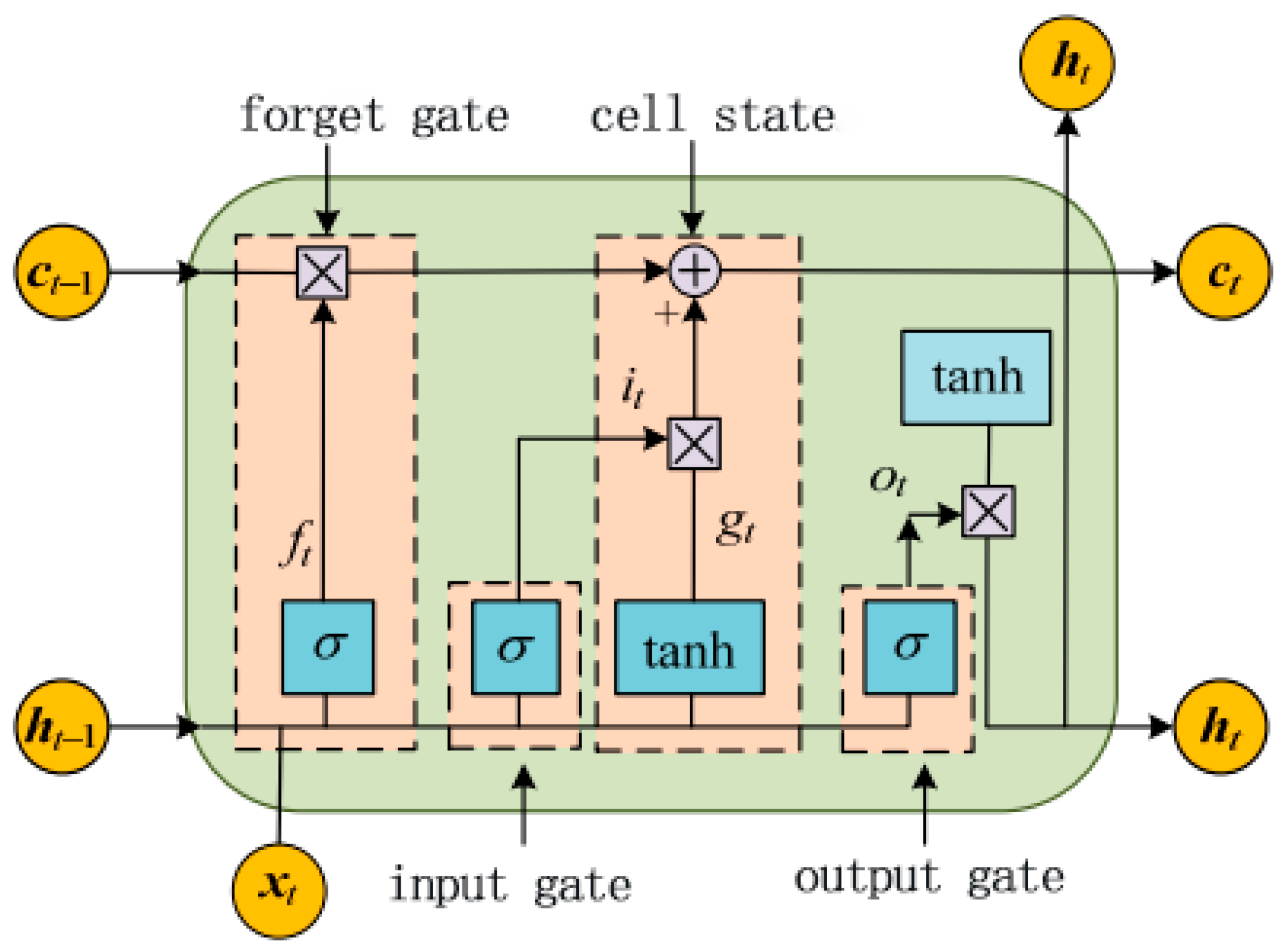
The main concept of the algorithm is based on some principles of quantum mechanics and a quantum-based model of the atom in which electrons move around the nucleus according to the orbits in which they are located. The AOS algorithm mainly simulates the trajectories of electrons affected by the electron density configuration and the energy absorbed or emitted by the electrons. Based on the fact that most previously developed optimization algorithms use a population of candidate solutions evolved from different stochastic processes, the proposed AOS algorithm considers many candidate solutions representing the electrons around the quantum nucleus ($X$). The search space in this algorithm is considered to be a cloud of electrons around the nucleus, which is divided into thin, spherical, concentric layers.

Each electron is represented by a solution candidate ($x_i^{}$) in the search space, while some decision variables ($x_i^j$) are also used to define the position of the solution candidate in the search space. The mathematical equation for this purpose is as follows.

$$\begin{array}{l}X=\left[\begin{array}{l}{X}_1\\ X_2\\ ⋮\\ X_i\\ ⋮\\ X_m\end{array}\right]=\left[\begin{array}{llllll}{X}_1^1& X_1^2& \cdots & X_1^j& \cdots & X_1^d\\ X_2^1& X_2^2& \cdots & X_2^j& \cdots & X_2^d\\ ⋮& ⋮& \cdots & ⋮& \ddots & ⋮\\ X_{{}_i}^1& X_i^2& \cdots & X_i^j& \cdots & X_i^d\\ ⋮& ⋮& \cdots & ⋮& \ddots & ⋮\\ X_{{}_m}^1& X_m^2& \cdots & X_m^j& \cdots & X_m^d\end{array}\right],\{\begin{array}{l}i=1,2,\dots ,m.\\ j=1,2,\dots ,d.\end{array}\\ \end{array}$$

(1)

where $m$ is the number of candidate solutions (electrons) within the search space (electron cloud) and $d$ is the problem dimension indicating the location of the candidates (electrons).

The initial position of the electrons inside the electron cloud is determined randomly according to the following mathematical equation.

$$x_i^j(0)=x_{i,\min }^j+rand\cdot (x_{i,\max }^j-x_{i,\min }^j),\{\begin{array}{l}i=1,2,\dots ,m.\\ j=1,2,\dots ,d.\end{array}$$

(2)

where $x_i^j(0)$ denotes the initial position of the candidate solution. $x_{i,\min }^j$ and $x_{i,\max }^j$ denote the minimum and maximum bounds for the $j$ th decision variable that is the $i$-th candidate solution. $rand$ is a uniformly distributed random number in the range [0,1].

It thinks electrons with higher energy levels are considered in the mathematical model as solution candidates with poorer objective function values according to the details provided for the quantum-based atomic model. The vector equation used to include the objective function values (energy levels) for different candidate solutions (electrons) is as follows.

$$E=\left[\begin{array}{l}{E}_1\\ E_2\\ ⋮\\ E_{\mathrm{i}}\\ ⋮\\ E_{\mathrm{m}}\end{array}\right],i=1,2,\dots ,m.$$

(3)

where $E$ is the vector containing the values of the objective function. $E_i$ is the energy level of the $i$-th candidate solution. m is the number of candidate solutions (electrons) within the search space (electron cloud).

To mathematically represent the imaginary layers around the nucleus, a random integer $n$ is assigned based on the number of spherical imaginary layers around the nucleus $L$. The layers produced in the imagination represent the wave-like behavior of the electrons around the nucleus. The layer $L_0$ with the smallest radius represents the position of the nucleus. The remaining layers $L_i$ represent the positions of the electrons, as shown in Figure 1.

The AOS algorithm used a log-normal Gaussian distribution function to build the mathematical model based on the quantum excitation model of the atom. Figure 2 represents the determined positions of the electrons (candidate solutions) with a log-normal Gaussian distribution function. In this distribution, the electron has a higher total presence probability layer ($L_1$ to $L_2$) in the second space than the first layer ($L_0$ to $L_1$), which represents the true wave-like behavior of the electron in the quantum-based model of the atom, as shown in Figure 2.

Each imaginary created layer contains several candidate solutions according to the details provided for determining the electronic location by PDF. The vectors containing $n$ objects in the different layers $X^k$ and their objective function $E^k$ values are represented as follows.

$$X^k=\left[\begin{array}{l}{X}_1^k\\ X_2^k\\ ⋮\\ X_i^k\\ ⋮\\ X_p^n\end{array}\right]=\left[\begin{array}{l}{X}_1^1{X}_1^2\cdots X_1^j\cdots X_1^d\\ X_2^1{X}_2^2\cdots X_2^j\cdots X_2^d\\ ⋮\\ X_i^1{X}_i^2\cdots X_i^j\cdots X_i^d\\ ⋮\\ X_p^1{X}_p^2\cdots X_p^j\cdots X_p^d\end{array}\right],\{\begin{array}{l}i=1,2,\dots ,m.\\ j=1,2,\dots ,d.\\ k=1,2,\dots ,n.\end{array}$$

(4)

$$E^k=\left[\begin{array}{l}{E}_1^k\\ E_2^k\\ ⋮\\ E_{{}_{\mathrm{i}}}^k\\ ⋮\\ E_p^n\end{array}\right],\{\begin{array}{l}i=1,2,\dots ,p.\\ k=1,2,\dots ,n.\end{array}$$

(5)

where $X_{{}^i}^k$ is the i-th candidate solution in the k-th virtual layer. $n$ is the maximum number of virtual creation layers. $p$ is the total number of candidate solutions in the k-th virtual layer. $d$ is the problem dimension. $E_{{}^i}^k$ is the objective function value of the $i$-th candidate solution in the k-th virtual layer.

The concepts of binding state and binding energy are mathematically modeled by considering the position vector’s average value and the candidate solution’s objective function value based on principles of the atomic orbital model. For each of the considered hypothetical layers, the binding states and binding energies are calculated as follows.

$$B{S}^k=\frac{{\displaystyle {\sum }_{i=1}^p{X}_i^k}}{p},\{\begin{array}{l}i=1,2,\dots ,p.\\ k=1,2,\dots ,n.\end{array}$$

(6)

$$B{E}^k=\frac{{\displaystyle {\sum }_{i=1}^p{E}_i^k}}{p},\{\begin{array}{l}i=1,2,\dots ,p.\\ k=1,2,\dots ,n.\end{array}$$

(7)

where $B{S}^k$ and $B{E}^k$ are the binding states and binding energies at the k-th level. $X_i^k$ and $E_i^k$ are the positions and objective function values of the i-th candidate solutions in the k-th level. In addition, $m$ is the total number of candidate solutions in the search space.

Since the total energy level of an atom is evaluated by considering the bound states and binding energies of all electrons, the mathematical representation of the average value of the position vector and the objective function of the candidate solution in the whole search space are as follows.

$$BS=\frac{{\displaystyle {\sum }_{i=1}^m{X}_i^{}}}{m},i=1,2,\dots ,m.$$

(8)

$$BE=\frac{{\displaystyle {\sum }_{i=1}^m{E}_i^{}}}{m},i=1,2,\dots ,m.$$

(9)

During the optimization process in the mathematical model of the AOS algorithm, specifically, the positions of the candidate solutions in the imaginary spherical layer are updated by considering the absorption or emission of photons and other interactions with particles, taking into account the energy levels of the electrons and the binding energy of the imaginary layer.

To facilitate the mathematical representation of the position update process in the AOS algorithm, each electron is assigned a randomly generated number $\varphi$ uniformly distributed in the range [0,1], in order to represent the probability of action of photon or other interactions. To distinguish between different electron interactions, a photon rate $PR$ parameter is introduced to represent the probability of different electron interactions. For $\varphi \ge PR$, photons act on electrons. In this case, the energy level $E_i^k$ of the $i$-th electron or candidate solution $X_i^k$ in the $k$ th layer is compared with the binding energy $B{E}_{}^k$ of the $k$-th layer. If $E_i^k\ge B{E}_{}^k$, the candidate solution (electron) emits a certain amount of energy (photon). Depending on the energy, the electron can reach the bound state $\mathrm{BS}$. In addition, the energy of the atom or even the lowest energy state in the atom is $\mathrm{LE}$. The step of updating the mathematical formula in this case is written as follows.

$$X_{i+1}^k=X_i^k+\frac{{\alpha }_i\times ({\beta }_i\times \mathrm{LE}-{\gamma }_i\times \mathrm{BS})}{k},\{\begin{array}{l}i=1,2,\dots ,p.\\ k=1,2,\dots ,n.\end{array}$$

(10)

where $X_{i+1}^k$ and $X_i^k$ are the current and future positions of the $i$-th candidate solution at the $k$-th level. $\mathrm{LE}$ is the candidate solution with the lowest energy level in the atom. $\mathrm{BS}$ is the bound state of the atom. In addition, ${\alpha }_i$, ${\beta }_i$ and ${\gamma }_i$ are vectors containing randomly generated numbers that are uniformly distributed in the range (0,1) for determining the emitted energy.

If the energy level of a candidate solution in a particular layer is lower than the binding energy ($E_i^k<B{E}_{}^k$) of that layer, the photon absorption energy is considered. In this process, the candidate solution tends to absorb photons with ${\beta }_{}$ and $\gamma$ the considered energy in order to reach both the bound state of the layer (${\mathrm{BS}}^k$) and the electronic state with the lowest energy level (${\mathrm{LE}}^k$) within the considered layer. The mathematical equation for the candidate solution position updating process in this process is as follows.

$$X_{i+1}^k=X_i^k+{\alpha }_i\times ({\beta }_i\times \mathrm{LE}-{\gamma }_i\times \mathrm{BS}),\{\begin{array}{l}i=1,2,\dots ,p.\\ k=1,2,\dots ,n.\end{array}$$

(11)

If the random generation number ($\varphi$) of each electron is less than $\mathrm{PR}$ ($\varphi <PR$), photons cannot act on the electrons, and therefore the movement of electrons between different layers around the nucleus is considered based on some other effects, such as interactions with particles or magnetic fields, which can also lead to energy absorption or emission. In this respect, the process of updating the position of solution candidates based on these effects is considered to be as follows.

$$X_{i+1}^k=X_i^k+r_i,\{\begin{array}{l}i=1,2,\dots ,p.\\ k=1,2,\dots ,n.\end{array}$$

(12)

where $r_i$ is a vector containing randomly generated numbers that are uniformly distributed in the range (0,1).

2.2. Basic LSTM

The long short-term memory network (LSTM) was proposed by Hochreiter and Schmidhuber. It solves the problem that RNNs suffer from long-term dependency and are unable to build predictive models for longer time spans. The LSTM network structure consists of input gates, forgetting gates, output gates and cell states. The basic structure of the network is shown in Figure 3.

LSTM is a special kind of recurrent neural network. It avoids the problem of gradient disappearance and gradient explosion caused by traditional recurrent neural networks by carefully designing the “gate” structure, and can effectively learn the long-term dependence relationship. Therefore, the LSTM model with memory function shows strong advantages in dealing with time series prediction and classification problems.

When the input sequence is set to $\left(x_1,x_2,\cdots ,x_T\right)$ and the hidden layer state is $\left(h_1,h_2,\cdots ,h_T\right)$, the equation at moment t is as follows.

$$f_t=\sigma \left(W_f\times \left[h_{t-1},x_t\right]+b_f\right)$$

(13)

$$i_t=\sigma \left(W_i\times \left[h_{t-1},x_t\right]+b_i\right)$$

(14)

$${\tilde{C}}_t=tanh\left(W_C\times \left[h_{t-1},x_t\right]+b_C\right)$$

(15)

$$C_t=f_t{C}_{t-1}+i_t{\tilde{C}}_t$$

(16)

$$o_t=\sigma \left(W_o\times \left[h_{t-1},x_t\right]+b_o\right)$$

(17)

$$h_t=o_{t}tanh\left(C_t\right)$$

(18)

where $x_t$ is the input vector of the LSTM cell. $h$ is the cell output vector. $f_t$, $i_t$, ${ \mathrm{o}}_t$ denote the forgetting gate, input gate and output gate, respectively. $C_t$ denotes the cell state. Subscript $t$ denotes the moment. $\sigma$, $tanh$ are the activation functions. $W$ and $b$ denote the weight and bias matrix, respectively.

The key to the LSTM is the cell state $C_t$, which is maintained in $t$ memory at all times and is regulated by forgetting gate $f_t$ and input gate $i_t$. The role of the forgetting gate is to allow the cell to remember or forget its previous state $C_{t-1}$. The role of the input gate is to allow or prevent the incoming signal from updating the cell state. The role of the output gate is to control the output and transfer of the cell state $C_t$ to the next cell. the internal structure of the LSTM cell is made up of multiple perceptron. The backpropagation algorithm is usually the most common training method.

2.3. Random Vector Functional Link Network (RVFL)

The backpropagation algorithm in ANN has the disadvantages of slow convergence and long learning time. In contrast, the RVFL neural network randomly assigns input weights and biases, uses least squares to train the output weights, and does not perform the connection of processing units in the same layer or the feedback connection between different layers, which can make up for the defects of ANN [43], with good nonlinear fitting ability. The model structure is shown in Figure 4.

In the following, each layer of the RVFL model is interpreted.

(1)

Input layer

The main role of the input layer is to input a training set $\left\{(x^n,y^n)\right\}$ with U training samples, $u=1,2,\dots ,U$; $x$ is the $n$-dimensional input variable, $x\in R^n$; $y$ is the desired output variable, $y\in R^U$. The analysis in this paper yields a training sample space of ${\left\{(x^{\tau },y^{\tau })\right\}}_{\tau =1}^U$, $x^{\tau }$ is the five-dimensional input variable at time $\tau$, $x^{\tau }=(T_{a_i}^{\tau },T_{e_i}^{\tau },T_{w_i}^{\tau },T_{a_{i,in}}^{\tau },T_{a_{i,out}}^{\tau })$; $y^{\tau }$ is the output variable at time $\tau$, $y^{\tau }=T_{e_i}^{\tau +1}-T_{e_i}^{\tau }$.

(2)

Hidden layer

The implicit layer can establish the activation function $h$ value of the output of each implicit layer node, which is obtained in this paper by the sigmoid function $h$, which serves to transform the input variables linearly and can be expressed as shown below.

$$h(x,w,b)=\frac{1}{1+\exp {\left\{-w^{T}x+b\right\}}^{\ast }}$$

(19)

where w and b are the weights and biases from the input layer to the hidden layer, respectively, independent of the training data, and are determined before, ultimately, the implicit layer kernel mapping matrix H is calculated as follows for the output layer component.

$$H=\left[\begin{array}{ccc}{h}_1(x_1)& \dots & h_L(x_1)\\ ⋮& \dots & ⋮\\ h_1(x_U)& \dots & h_L(x_U)\end{array}\right]$$

(20)

where L denotes the number of nodes in the hidden layer.

(3)

Output layer

Calculating the weights from the hidden layer to the output layer $\beta$ is a central part of the learning process of the RVFL neural network, and according to the standard regularized least squares principle to find $\beta$.

$${\beta }^{*}=\underset{\beta ÎR}{\arg \min }\frac{1}{2}{\Vert H\beta -Y\Vert }_2^2+\frac{\lambda }{2}{\Vert \beta \Vert }_2^2\lambda >0$$

(21)

where Y is a column vector $y^u$ consisting of the training sample space corresponding to $x^u$; $\lambda$ denotes a constant. The final weights $\beta$ can be obtained as demonstrated below.

$$\beta ={(H^{T}H+\lambda I)}^{-1}{H}^{T}Y$$

(22)

where I denotes the unit matrix. At this point, the learning process is complete and the test output of the RVFL model is obtained, as shown below.

$$\widehat{y}={\displaystyle \sum _{l=1}^L{\beta }_{l}h(x,{\omega }_l,b_l)}$$

(23)

The RVFL model has a rapid convergence speed and a short learning time.

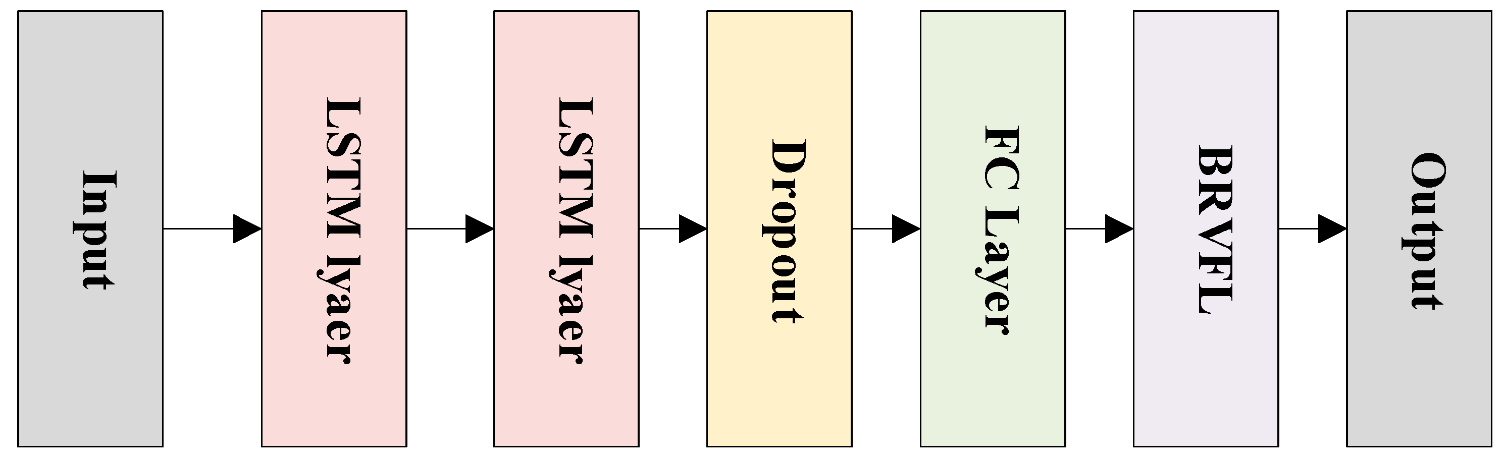
3. Reservoir Prediction Model Based on ILSTM-BRVFL

This section will be divided into four subsections. It will provide a concise and precise description of the ILSTM-BRVFL.

3.1. Improved Atomic Orbital Search Algorithm (IAOS)

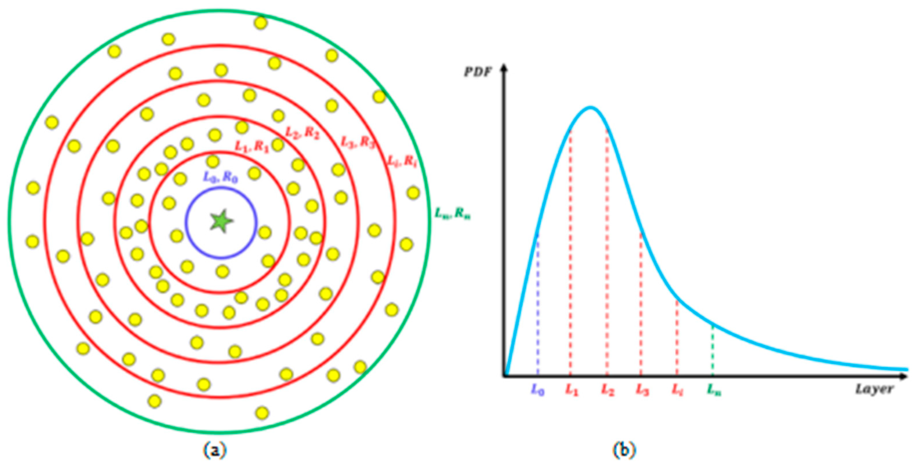
3.1.1. Population Initialization Based on Chaos Theory

Chaotic mapping is a nonlinear theory with nonlinearity, universality, ergodicity, and randomness characteristics. It can traverse all states without repetition within a certain range according to its properties and can help generate new solutions and increase population diversity in intelligent algorithm optimization. Therefore, it is widely used [44]. Tent mapping iterates fast, and the chaotic sequence is uniformly distributed between [0,1] with the expression as follows.

One of the widely used mapping mechanisms in chaos theory research is chaos mapping $Tent$ with fast iteration and a mathematical iteration equation as follows.

$${\lambda }_{t+1}=\{\begin{array}{l}{\lambda }_t/\alpha ,{\lambda }_t\in [0,\alpha ,)\\ (1-{\lambda }_t)/(1-\alpha ),{\lambda }_t\in [\alpha ,1)\end{array}t=0,1,2,\cdots ,T$$

(24)

where ${\lambda }_t$ is the amount of chaos generated at the t-th iteration. $T$ is the maximum number of iterations. $\alpha$ is a constant between [0,1]. We chose 0.6 in this paper, which is the best chaotic state at this time.

3.1.2. Position Updating Based on Individual Memory Function

In the exploration phase of the AOS algorithm, analysis of Equation (1) shows that only the current position information of the electron individual is considered in the iterative position update process, which converges to the optimal solution by the random movement of the electron individual. It indicates that its development phase is an algorithm lacking the position memorability of the electron itself. To improve the local development capability of the AOS algorithm, inspired by the particle swarm optimization (PSO) algorithm, the idea of memory preservation of the optimal solution of the particle’s own motion history in the PSO algorithm is introduced into the AOS algorithm. In addition, the memory function of the individual is improved so that it can remember the lowest energy position in the process of its own movement. To this end, this paper proposes a position update formula based on the memory function of the electron individual itself to replace Equation (12), expressed as follows.

$$X_{i+1}^k=b_1(X_i^k+r_i)+b_2\cdot rand\cdot (X_{HI}^k-X_i^k),\{\begin{array}{l}i=1,2,\dots ,p.\\ k=1,2,\dots ,n.\end{array}$$

(25)

where $b_1,b_2\in [0,1]$ is the individual memory coefficient. rand is a random number between [0,1]. In addition, $X_{HI}^k$ is the lowest energy position experienced by the k-th electron. Similar to PSO algorithm, the effect of individual memory on the ability to develop the algorithm can be reconciled by adjusting the value of b₁, b₂.

The main process of the IAVOA algorithm is as follows.

(1)

Initialize the population, initialize the population size m, candidate positions x_i, fitness function E_i, determine the binding state (BS) and binding energy (BE) of the atom, determine the candidate atom with the lowest energy level (LE) in the atom, maximum number of iterations (Maximum).

(2)

Sort the candidate solutions in ascending or descending order to form the solution space by probability density function (PDF).

(3)

Global exploration according to Equations (10) and (11) and local exploitation according to Equation (25).

(4)

The maximum number of iterations is reached, and the output is saved.

The pseudocode of the IAOS is shown in Algorithm 1.

Algorithm 1 IAOS

Inputs: The population size m, initial positions of solution candidates (xi) based on chaos theory, Evaluate fitness values for initial solution candidates, determine binding state (BS) and binding energy (BE) of atom, determine candidate with lowest energy level in atom (LE) Outputs: The lowest energy level in atom (LE)       While Iteration < Maximum number of iteration       Generate n as the number of imaginary layers       Create imaginary layers       Sort solution candidates in an ascending or descending order       Distribute solution candidates in the imaginary layers by PDF         For k = 1:n         Determine the binding state ($B{S}^k$) and binding energy ($B{E}^k$) of the kth layer            Determine the candidate with lowest energy level in the kth layer ($L{E}^k$)             For i = 1:p                 Generate  $\phi ,\alpha ,\beta ,\gamma$                 Determine PR                 If  $\phi \ge PR$                     If  $E_i^K\ge B{E}^k$                          Run Equation (10)                     Else if  $E_i^K<B{E}^k$                          Run Equation (11)                     End                 Else if  $\phi <PR$                       Run Equation (25)                  End             End         End         Update binding state (BS) and binding energy (BE) of atom          Update candidate with lowest energy level in atom (LE)       End while

3.2. LSTM Based on Improved IAOS (ILSTM)

As mentioned in the previous section, the parameters of the basic LSTM model are artificially specified, which directly affects the prediction effect of the model. For this reason, we propose an improved IAOS-LSTM model, the main idea of which is to use the good parameter-finding ability of the above IAOS algorithm to optimally match the relevant parameters of the LSTM to improve the prediction effect of the LSTM. The IAOS-LSTM model modeling process is as follows.

(1)

Initialize the relevant parameters, and initialize the IAOS algorithm parameters: population size, fitness function, and other parameters assigned. Initialize the LSTM algorithm parameters: set the time window, set the initial number of neurons in the two-layer hidden layer, the initial learning rate, the initial number of epochs, and the batch size. In addition, the error is used as the fitness function in this paper with the following expressions.

$$fitness=1-\mathrm{acc}(f;D)=1-\frac{1}{m}{\displaystyle \sum _{i=1}^{m}I}\left(f\left(x_i\right)=y_i\right)$$

(26)

where D denotes the training set, m is the number of samples in the training set, $f\left(x_i\right)$ is the predicted sample label, $y_i$ is the original sample label, and $I(f\left(x_i\right)=y_i)$ is a function that takes the value of 1 if $f\left(x_i\right)=y_i$ and 0 otherwise.

(2)

Set the LSTM parameters to form the corresponding particles according to the need, and the particle structure is ($alpha$, $num\_epochs$, $batch\_size$, $hidden\_nodes0$, $hidden\_nodes1$), where $alpha$ denotes the LSTM learning rate, $num\_epochs$ denotes the number of iterations, $batch\_size$ denotes the packet size, $hidden\_nodes0$ denotes the number of neurons in the first hidden layer of LSTM, $hidden\_nodes1$ denotes the number of neurons in the second hidden layer of LSTM, and the above particles are the IAOS optimized LSTM super parameters.

(3)

The electron energy is updated according to Equation (10), and then the fitness value is calculated according to the new electron energy, and the lowest energy electron individual optimal solution is updated.

(4)

If the number of iterations reaches the maximum number of 100 iterations, the predicted values are output for the trained LSTM model according to the optimal solution, and if the number of iterations does not reach the maximum, the process (3) is returned to continue iterating.

(5)

The optimal hyper-parameters are brought into the LSTM model, which is the IAOS-LSTM model.

The pseudocode flow of IAOS optimized LSTM is shown in Algorithm 2.

Algorithm 2 Pseudocode of IAOS optimized LSTM

Input: Training samples set: trainsets, LSTM initialization parameters

Output: IAOS-LSTM model

1. Initialize the LSTM model:

assign parameters range = [lr,epoch,batch_size,hidden0,hidden1,] = [0.0001–0.01,25–100,0–256,0–128,0–128];

loss = ‘categorical_crossentropy’, optimizer = adam

2. Set IAOS equalization parameters and Import trainsets to Optimization:  parameters para = [lr,epoch,batch_size,hidden0,hidden1,]  ${\overrightarrow{C}}_{ave}$= fitness = 1-acc = Error Equation (26) num_iteration = 100 IAOS-LSTM = LSTM(IAOS(para),trainsets) save model:save(‘IAOS-LSTM’) return para_best to LSTM model

3.3. Bidirectional RVFL (BRVFL)

Since the input weights and the deviations of the hidden layer neurons of RVFL are obtained randomly, the hidden layer output matrix often has pathological problems when there are outlier points or perturbations in the training data population, making the overall generalization performance and prediction accuracy of the network degraded. Although the RVFL algorithm has fast learning speed and good generalization performance, it is necessary to artificially set the number of hidden layer nodes before training starts. As a key research element in SLFNs, the number of hidden layer nodes has been an important factor affecting the performance of the algorithm. To address this problem and further improve the learning efficiency and reduce the number of hidden nodes and computational cost, this section proposes a BRVFL based on the RVFL algorithm, drawing on the ideas of incremental extreme learning machine (I-ELM) and bidirectional extreme learning machine (B-ELM).

In the mechanism of BRVFL, when the number of hidden nodes is odd, the hidden node parameters are generated randomly. In addition, when the number of hidden nodes is even, the hidden node parameters are determined by an appropriate error function. In this way, hidden nodes can be added automatically until the model meets a given accuracy or the number of hidden nodes exceeds a given maximum. The B-ELM algorithm is detailed as follows.

The objective function $f_B$ is assumed to be continuous, and $H_{2n+1}^r$ is a sequence of randomly generated functions, and a sequence of error feedback functions $H_{2n}^e,n\in Z$ is obtained. For a neural network $f_{Bn}$ containing $n$ hidden layer nodes, the residual error function is $e_n=f_B-f_{Bn}$. When the number of hidden layer nodes $L\in \left\{2n+1,n\in Z\right\}$, the hidden node parameters $a_{2n+1}$ and $b_{2n+1}$ are determined randomly in the BRVFL.

$$H_{2n+1}^r=H(a_{2n+1},b_{2n+1},x)$$

(27)

$${\beta }_{2n+1}^{}=\frac{\langle e_{2n},H_{2n+1}^r\rangle }{{\Vert H_{2n+1}^r\Vert }^2}$$

(28)

When the number of nodes in the implicit layer $L\in \left\{2n,n\in Z\right\}$, the implicit node parameters $a_{2n}$ and $b_{2n}$ are as follows.

$$H_{2n}^e=e_{2n-1}{({\beta }_{2n-1})}^{-1}$$

(29)

$$a_{2n}^{}=g^{-1}(U(H_{2n}^e))\cdot x^{-1}$$

(30)

$$b_{2n}^{}=\sqrt{mse(g^{-1}(U(H_{2n}^e))-a_{2n}\cdot x}$$

(31)

$${\widehat{H}}_{2n}^e=U^{-1}(g(a_{2n}\cdot x+b_{2n}))$$

(32)

$${\beta }_{2n}^{}=\frac{\langle e_{2n-1},{\widehat{H}}_{2n}^e\rangle }{\Vert {\widehat{H}}_{2n}^e\Vert }$$

(33)

where $U:R\to [0,1]$ is the normalization function. $g^{-1}$ and $U^{-1}$ are the pseudo-inverse matrices of $g$ and $U$, respectively. The algorithm of BRVFL is summarized as shown in Algorithm 3.

Algorithm 3 Pseudocode of BRVFL

Input: training set: ${\left\{x_i,y_i\right\}}_{i=1}^{M_s}$; Maximum number of hidden layer neurons. $L_{\max }$ Hidden layer mapping function $g(x)$; training accuracy: ${\epsilon }_{BRVFL}$.

Output: The trained BRVFL model parameters

Recursive training process.

Initial error matrix $E_B=Y$, initial hidden layer node $L=0$

When $L<L_{\max }$, and $\Vert E_B\Vert \ge {\epsilon }_{BRVFL}$.

Set. $L=L+1$

If $L\in \left\{2n+1,n\in Z\right\}$

1. Random selection of neuron parameters and $a_{2n+1}$$b_{2n+1}$.

2. Calculate the randomly generated function sequence according to $H_{2n+1}^r$Equation (27),

3. Calculate the output weight according to ${\beta }_{2n+1}^{}$Equation (28)

If $L\in \left\{2n,n\in Z\right\}$

4. Calculate the error return function according to $H_{2n}^e$Equation (29)

5. Calculate the input weight and $a_{2n}$bias $b_{2n}$according to Equations (30) and (31).

6. Update ${\widehat{H}}_{2n}^e$according to Equation (32)

7. Calculate the output weight according to ${\beta }_{2n}^{}$Equation (33)

After adding a new node, calculate the error $E_B$

$E_B=E_B-G_L{\beta }_L$

When  $L=L_{\max }$  End

3.4. Actual Application in Oil Layer Prediction

Oil layer prediction is a critical research work in oil logging. To improve the accuracy of oil layer prediction, we propose an ILSTM-BRVFL neural network model by analyzing ILSTM and BRVFL networks. The algorithm combines ILSTM and BRVFL neural networks to make predictions on the dataset. That is, this model has the ability of ILSTM to perform fast and accurate feature extraction and the excellent prediction performance of the BRVFL method. The algorithmic model uses ILSTM as a feature extraction tool to extract data features. In addition, BRVFL is then used to predict the results of the extracted features instead of the SoftMax layer of LSTM. Since BRVFL possesses a simpler structure than the RVFL model with the same accuracy, it reduces the running time and improves its stability. The model structure of ILSTM-BRVFL (without IAOS) is shown in Figure 5. The pseudocode of ILSTM-BRVFL is shown in Algorithm 4. The flowchart of oil layer prediction is shown in Figure 6.

As shown in Figure 5, the model comprises two LSTM layers, a dropout layer, FC layer, and BRVFL. The IAOS algorithm is used to optimize the hyper-parameter of the model.

Algorithm 4 Pseudocode ofILSTM-BRVFL

Input: Training set, test set, parameters of IAOS

Assign hyper-parameters range of ILSTM-BRVFL model = [lr,epoch,batch_size,hidden0,hidden1] = [0.0001–0.01,0–128,0–256,0–256,0–256], T = 80, population of IAOS = 30, dim of IAOS = 5, k = 5, loss of ILSTM-BRVFL model = ‘categorical_crossentropy’, optimizer of ILSTM-BRVFL model = adam, Dropout = 0.5

Output: ILSTM-BRVFL model, test set accuracy, best hyper-parameters of ILSTM-BRVFL model.

1. use k-fold cross validation to split the training set into five identical data sets

For t = 1:k  Use four of the five data sets in the training set as the training set, one as the Validation Set, and select a different one of the five as the Validation Set each iteration time.

2. Initialize the population of IAOS value based on the hyper-parameters range of ILSTM-BRVFL model:

3. Calculate the fitness function based on Equation (26) and find the current optimal solution

While t1< T    For i = i: dim    Determine particle state and update particle position    End for    Updating the hyper-parameters of ILSTM = BRVFL models to predict Validation Set accuracy    t1 = t1 + 1    End while    End for    Record the best hyper-parameters of ILSTM = BRVFL models.    Build the ILSTM-BRVFL model    Use the ILSTM-BRVFL model to predict Test set.

As in the algorithmic procedure of ILSTM-BRVFL in Algorithm 4, we optimize the hyperparameters using the IAOS algorithm proposed in this paper and introduce K-fold cross-validation to verify the generalization performance of the model. The K value of K-fold cross-validation is 5.

Oil layer prediction has four main processes as follows.

(1)

Data collection and normalization

In the actual logging, the collected logging data are classified into two categories. One is the labeled data obtained by core sampling and laboratory analysis, which is generally used as the training set. The other is the unlabeled logging data, which are the data to be predicted or forecasted, i.e., the test set. In data pre-processing, denoising is the main operation. In addition, because the attributes have different magnitudes and different value ranges, these data need to be normalized first so that the sample data range is between [0,1]. In addition, the normalized influence factor data are substituted into the network for training and testing to produce the results. One of the formulas for sample normalization is shown below.

$$\overline{x}=\frac{\left(x-x_{\min }\right)}{x_{\max }-x_{\min }}$$

(34)

where $x\in \left[x_{\min },x_{\max }\right]$, $x_{\min }$ is the minimum value of the data sample attribute. In addition, $x_{\max }$ is the maximum value of the data sample attribute.

(2)

Selection of the sample set and attribute simplification

The selection of the sample set used for training should be complete and comprehensive and should be closely related to the formation assessment. In addition, since the degree of determination of each condition attribute of the formation varies for the prediction of the formation. There are dozens of logging condition attributes in the logging data, but not all of them play a decisive role. Therefore, attribute approximation is necessary. In this paper, we use an inflection point-based discretization algorithm followed by an attribute dependence-based reduction method to reduce the logging attributes [45].

(3)

ILSTM-BRVFL modeling

Firstly, the ILSTM-BRVFL model is established, and the activation function, number of hidden layer nodes, population size, and number of epochs in LSTM and RVFL are determined. In addition, the information of the training set after attribute reduction is input and the model’s hyper-parameters are trained using the training set based on k-fold cross-validation. The prediction result error rate in the training sample is used as the fitness function, see Equation (26).

(4)

Comparison of algorithm results

The trained ILSTM-BRVFL model was used to predict the test set and output the results. To verify the validity and stability of the models, we used the Catboost, Xgboost, pre-built RVFL, BRVFL, LSTM-BRVFL, ILSTM-BRVFL (PSO), ILSTM-BRVFL (MPA), and ILSTM-BRVFL (AOS) models as the subjects of comparison experiments.

4. Experiment and Result Analysis

4.1. Experimental Settings and Algorithm Parameters

The experimental environment is a PC with the following configuration: Windows 10 64-bit, Intel Core i5-3210M 2.50 GHz (Intel, Mountain View, CA, USA), 16 G RAM, and the programming software is MATLAB 2018b (MathWorks, Natick, MA, USA).

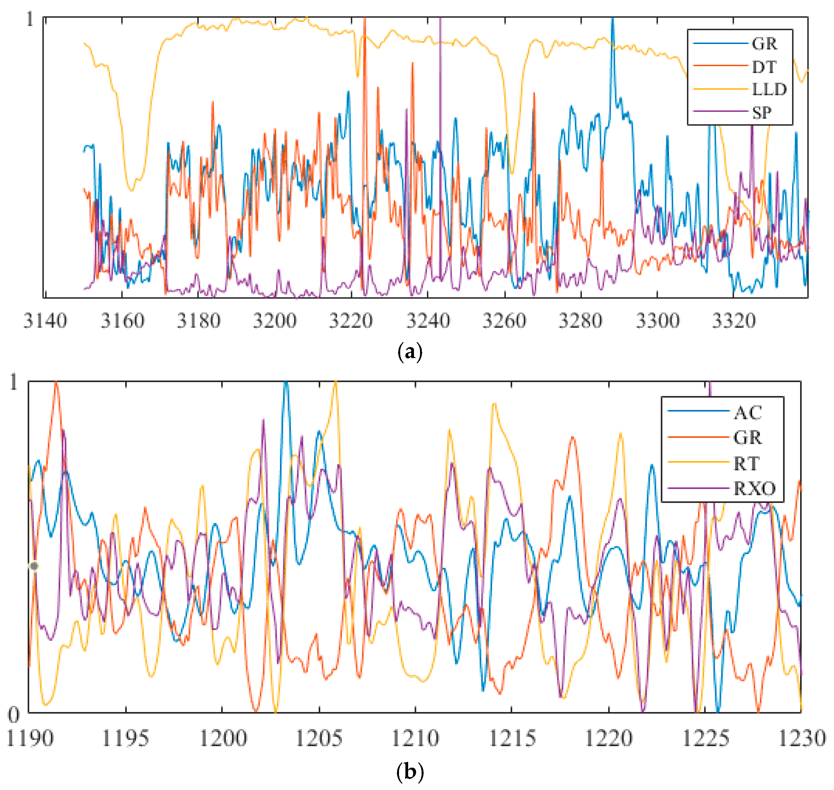
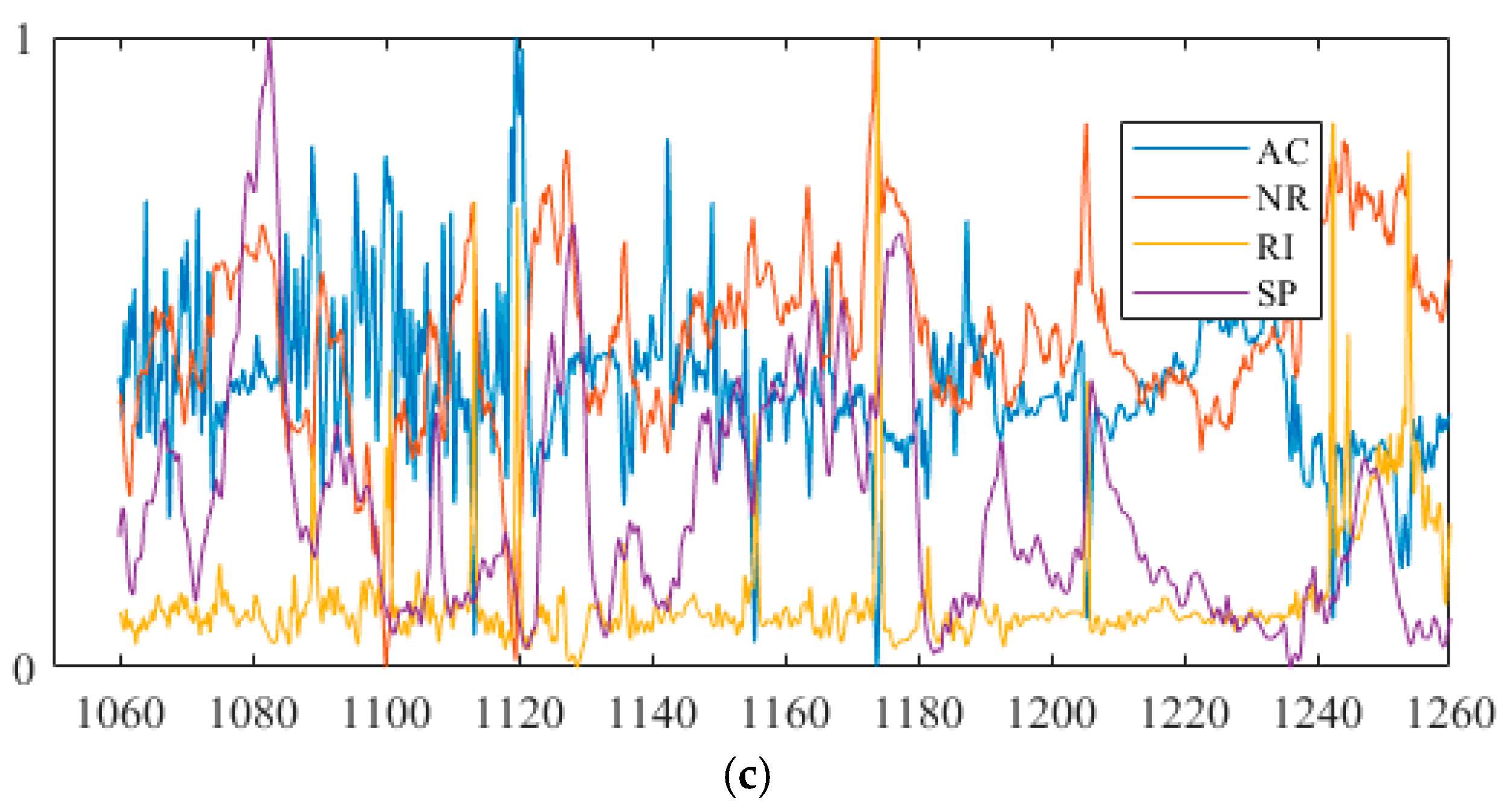
4.2. Data-Sets of Oil Layer Preparation

To verify the effectiveness of the model in real logging prediction, three sets of logging data from different wells were selected for training and prediction.

Table 1. Reduction results of logging data.

Well	Attribute
Original Attribute (w1)	GR, DT, SP, WQ, LLD, LLS, DEN, NPHI, PE, U, TH, K, CALL
Reduction results (w1)	GR, DT, SP, LLD, LLS, DEN, K
Original Attribute (w2)	AC, CNL, DEN, GR, RT, RI, RXO, SP, R2M, R025, BZSP, RA2, C1, C2, CALI, RINC, PORT, VCL, VMA1, VMA6, RHOG, SW, VO, WO, PORE, VXO, VW, so, rnsy, rsly, rny, AC1
Reduction results (w2)	AC, GR, RT, RXO, SP
Original Attribute (w3)	AC, CALL, GR, NG, RA2, RA4, RI, RM, RT, RXO, SP
Reduction results (w3)	AC, NG, RI, SP

shows the attribute simplification results for the data. These attributes are the valuable ones extracted from a large number of redundant conditional attributes, which also simplifies the complexity of the algorithm. The attribute reduction results of the logging data are shown in Table 1, and

Table 2. Detail of logging data.

Well	Training Set			Test Set
	Depth (m)	Oil Layers	Dry Layers	Depth (m)	Oil Layers	Dry Layers
w1	3150~3340	112	1238	3340~3470	92	810
w2	1190~1230	65	430	1230~1300	63	330
w3	1160~1260	55	800	1260~1300	79	105

shows detailed data-set information on logging data. The Figure 7 shows the logging curves normalized by attribute reduction of the training set, with the horizontal and vertical axes indicating the depth and standard values, respectively.

Table 1 lists the ranges of each property after the actual well properties are approximately reduced, where GR is natural gamma, DT is an acoustic time difference, SP is natural potential, LLD is deep lateral resistivity, LLS is shallow lateral resistivity, DEN is compensation density, K is potassium, NG is neutron gamma, and RI is intrusive layer resistivity, AC is acoustic wave, RT is true formation resistivity, RXO is flushed zone formation resistivity, NG is neutron-gamma, and RI is invaded zone resistivity.

Table 2 shows the detail datasets of logging data. The training set is used to train the ILSTM-BRVFL model, and test sets are used to evaluate the performance of the model.

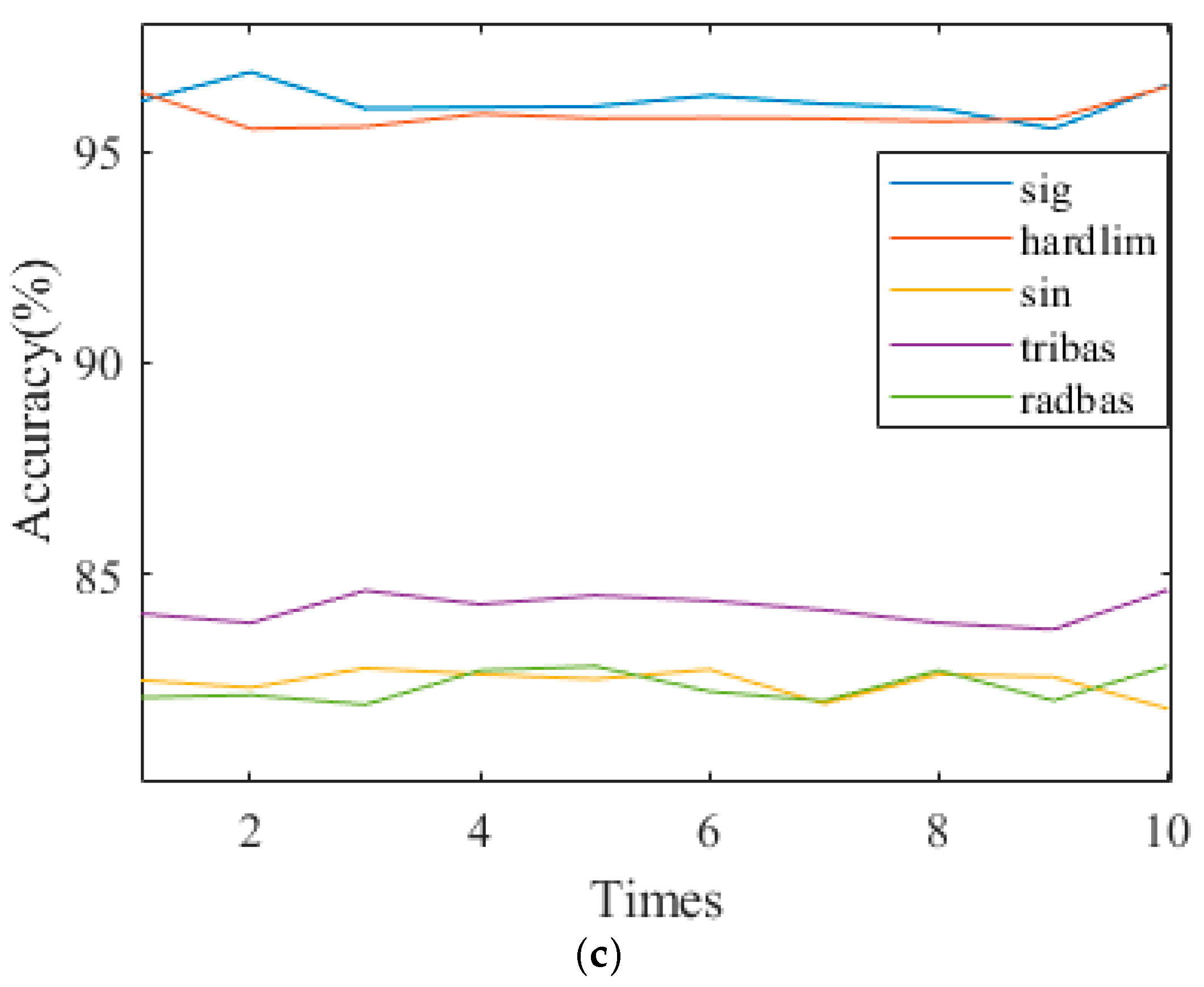
4.3. Selecting the Activation Function of the RVFL

A critical parameter affecting the prediction results of RVFL is its activation function. To verify the importance of the activation function in this experiment, the output results of different activation functions are compared again. Figure 8 shows the output of ILSTM-BRVFL using different activation functions for the three logs. Each output is averaged over ten independent experiments. As can be seen from the plots of the three logs, overall, the sigmoid and hardlim functions as activation functions produce much higher outputs than the sin, tribas, and radbas functions, by an average of 10–20%. The sigmoid function is slightly higher than hardlim at the beginning of the operation. The output of sigmoid is slightly higher than the output of the sigmoid. As the model time increases, sigmoid becomes better than or equal to hardlim. Therefore, the sigmoid was chosen as the final activation function in this experiment.

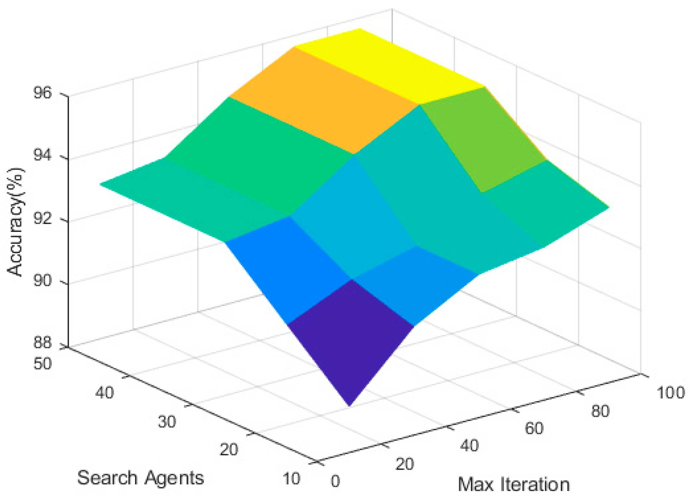
4.4. Research on the Parameters of the IAOS Algorithm

To explore the effect of IAOS parameters on the model, ablation experiments were conducted on the number of iterations and population size. The accuracy of the logging data was compared to the algorithm under different combinations of parameters, and this experiment was presented as a 3D graph using the well w₁ data as input, as shown in Figure 9.

From Figure 9, we can find that the model’s prediction accuracy rises with the number in the population and the number of iterations. The higher the number of particles randomly distributed in the search range, the better the search ability and the higher the model output accuracy. At the same time, as the number of iterations of the model increases, the more mature the structure of the model becomes, and the higher and smoother the prediction accuracy becomes. At the same time, the number of particles is not as high as it should be. For an algorithm, an increase in the number of particles also means an increase in the amount of computation. Losing a large amount of computation to obtain higher accuracy is not worth the cost. The same holds true for the number of iterations. In addition, we know that a linear increase in the number of iterations can lead to overfitting problems. Therefore, we find a critical value. As can be seen from the graph, the optimal values for population size and number of iterations are 30 and 80. At this point, the best results are achieved, with the least amount of computation cost.

4.5. Set Parameters of the Whole Algorithm

Based on the above experiments, the relevant parameters of the model are derived, and

Table 3. Set the final parameters of the algorithm.

Algorithm	Parameters
PSO	Population Size = 30, Maximum Iteration = 80, ω0 = 0.7, c1 = c2 = 1.5, dim = 5
MPA	Population Size = 30, Maximum Iteration = 80, FADs Effect coefficient = 0.2, p = 0.5 dim = 5
AOS	Population Size = 30, Maximum Iteration = 80, dim = 5
IAOS	Population Size = 30, Maximum Iteration = 80, dim = 5
LSTM	Maximum number of training rounds: Maxpochs = 50, hidden_size = 256 Learning rate:initialLearnRate = 0.001, Optimization method: adam Size of mini-bath:MiniBathSize = 64
RVFL	Number of hidden layer nodes: Number of Hidden Neurons = 105 Number of input layer nodes: Number of input Neurons = Number of training set samples, Activation function: sigmoid
ILSTM-BRVFL	hyper-parameters range of ILSTM-BRVFL model = [lr,epoch,batch_size,hidden0,hidden1] = [0.0001–0.01,0–128,0–256,0–256,0–256] loss of ILSTM-BRVFL model = categorical_crossentropy, optimizer of ILSTM-BRVFL model = adam, Dropout = 0.5

shows the final parameters set of the whole algorithm.

4.6. Evaluation Indicators of the Algorithm

To make the algorithm proposed in this paper more convincing, we use Macro-P, Macro-R, Macro-F1 and Accuracy to evaluate the performance of the algorithm. Macro-P is the number of samples predicted to be positive and correctly predicted divided by the number of samples predicted to be positive, Macro-P is the number of correctly predicted samples with a prediction of positive divided by the number of samples with a true case of positive, Macro-F1 can be regarded as a weighted average of model accuracy and recall, Accuracy is the total number of correctly identified individuals divided by the total number of identified individuals. The equations of those evaluation indicators are shown below.

$$Marco-R=\frac{TP}{TP+FN}$$

(35)

$$Macro-P=\frac{FP}{FP+TN}$$

(36)

$$Macro-F1=\frac{2}{1/Marco-R+1/Marco-P}$$

(37)

$$accuracy=\frac{TP+TN}{TP+FP+TN+FN}$$

(38)

where TN is the number of negative examples of correctly classified labels, and FP is the number of positive examples of incorrectly classified labels, and TP is the number of positive examples of correctly classified labels, and FN is the number of negative examples of incorrectly classified labels.

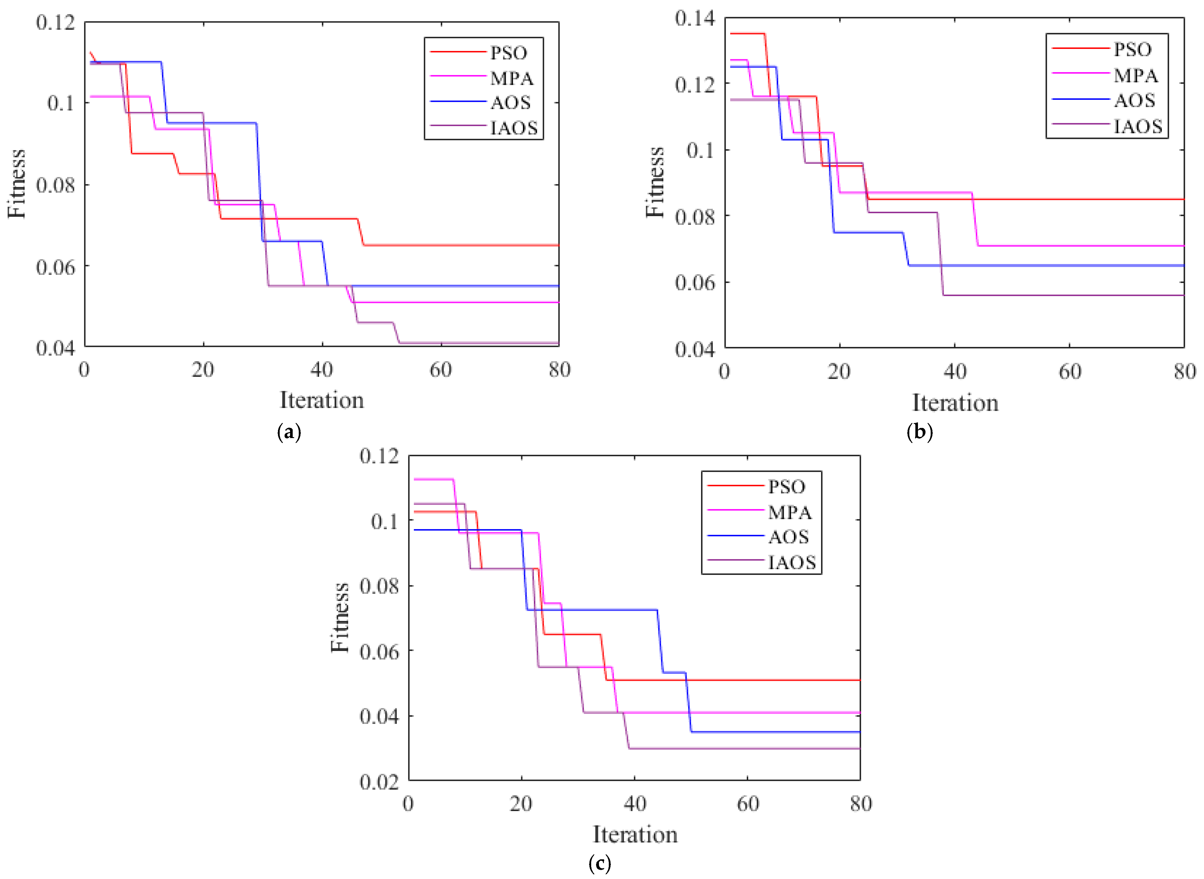
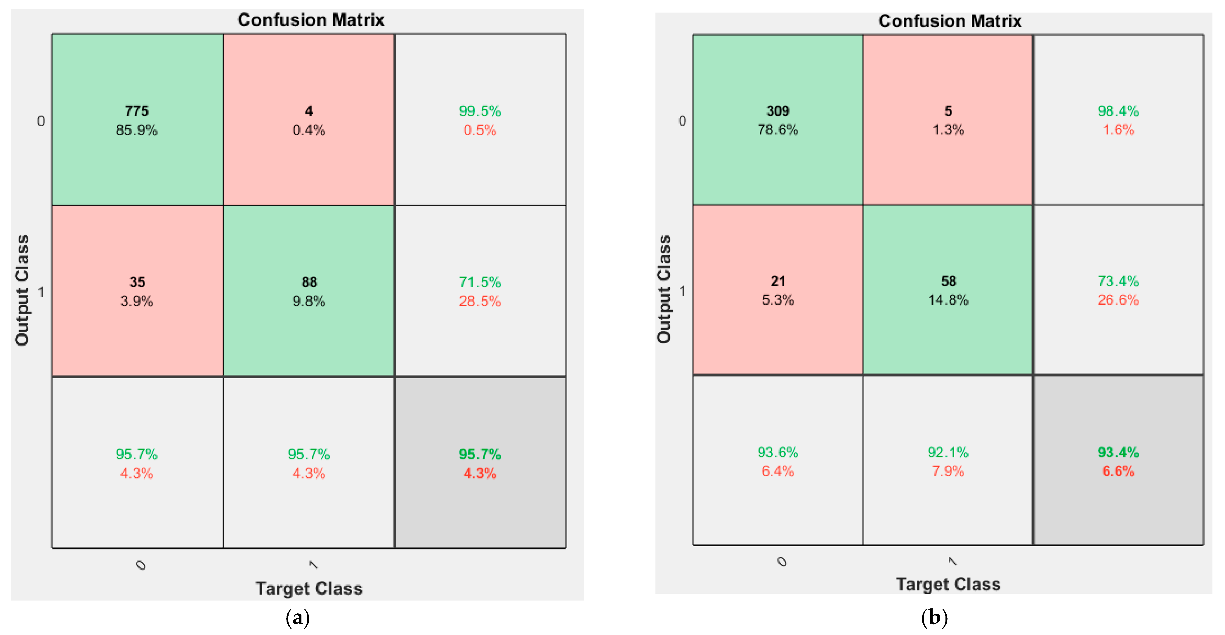
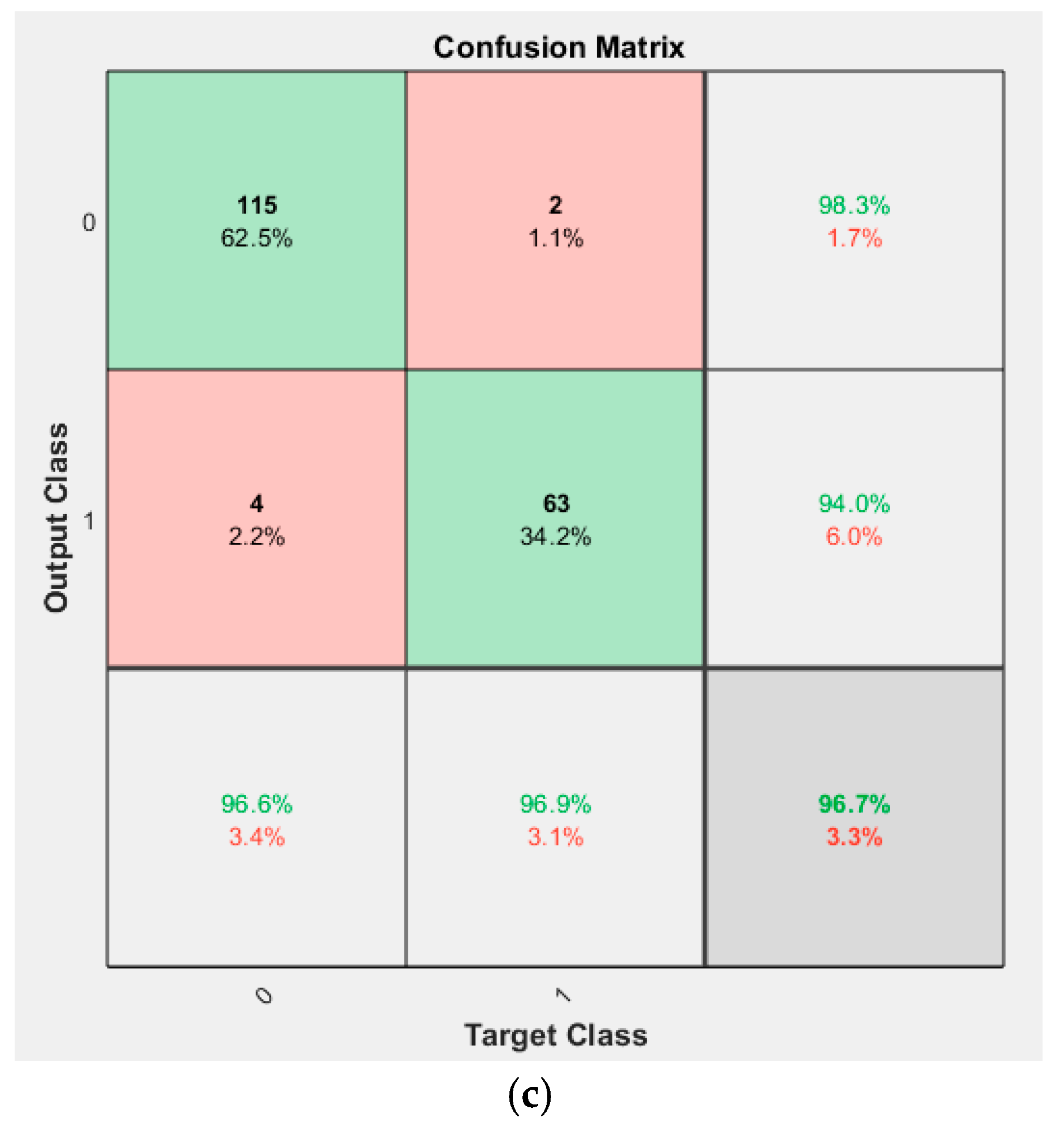
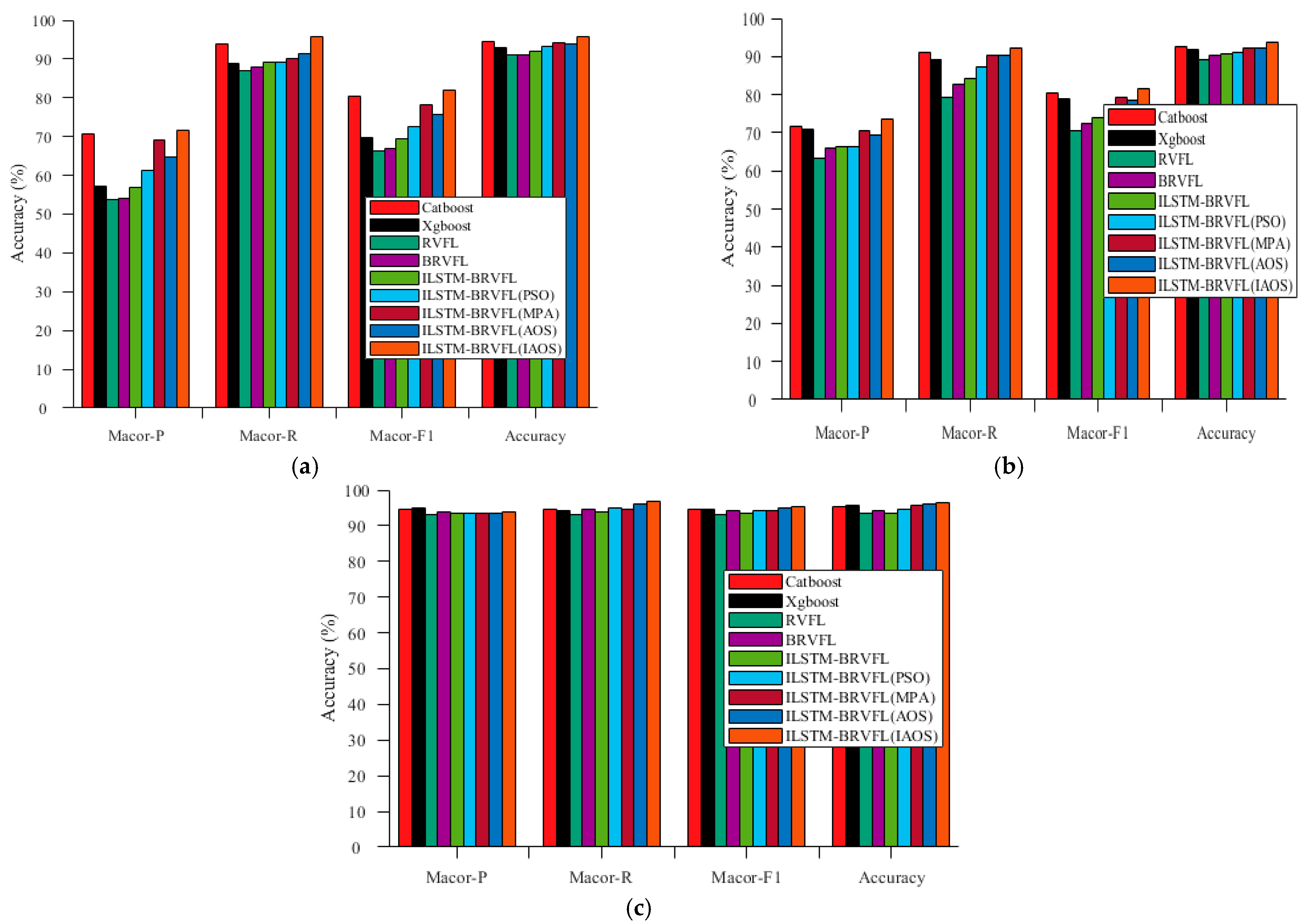
4.7. Discussion of the Algorithm Results

In this study, the parameters of each algorithm model and the total dimensionality of the test set features during the training process were compared and the corresponding evaluation metrics were calculated to evaluate the algorithms. The best hyper-parameter of the ILSTM-BRVFL model on three well logging data sets are shown in

Table 4. Set the final parameters of the algorithm.

well	Learing Rate	Epoch	Batch_size	Hidden0	Hidden1
w1	0.0091	56	212	125	178
w2	0.0012	45	185	138	154
w3	0.0095	63	176	98	167

. The loss vs. number of epochs on the training and validation datasets of based on best hyper-parameter are shown in Figure 10. The convergence curve between PSO, MPA, AOS, and IAOS when using the optimal ILSTM-model are shown in Figure 11. The confusion matrix for the best test set results of the three sets of logging data using the proposed algorithm is shown in Figure 12. The evaluation metrics for the three sets of logging data under each comparison model are presented in

Table 5. Evaluation indicators of the contrast model on w₁.

	Macro-P%	Macro-R%	Marco-F1%	Accuracy%
Catboost	70.68	93.82	80.40	94.45
Xgboost	57.25	88.88	69.64	93.01
RVFL	53.69	86.95	66.38	91.05
BRVFL	54.00	88.04	66.94	91.17
LSTM-BRVFL	56.94	89.13	69.49	92.02
ILSTM-BRVFL (PSO)	61.20	89.13	72.57	93.12
ILSTM-BRVFL (MPA)	69.17	90.21	78.30	94.28
ILSTM-BRVFL (AOS)	64.61	91.30	75.67	93.98
ILSTM-BRVFL (IAOS)	71.52	95.71	81.86	95.63

,

Table 6. Evaluation indicators of the contrast model on w₂.

	Macro-P%	Macro-R%	Marco-F1%	Accuracy%
Catboost	71.63	91.24	80.25	92.62
Xgboost	70.89	89.35	79.05	91.85
RVFL	63.29	79.37	70.42	89.31
BRVFL	65.82	82.54	72.38	90.36
LSTM-BRVFL	66.25	84.12	74.12	90.51
ILSTM-BRVFL (PSO)	66.26	87.30	75.34	90.94
ILSTM-BRVFL (MPA)	70.37	90.47	79.16	92.36
ILSTM-BRVFL (AOS)	69.51	90.47	78.62	92.02
ILSTM-BRVFL (IAOS)	73.41	92.13	81.73	93.63

and

Table 7. Evaluation indicators of the contrast model on w₃.

	Macro-P%	Macro-R%	Marco-F1%	Accuracy%
Catboost	94.51	94.65	94.57	95.33
Xgboost	94.93	94.28	94.60	95.85
RVFL	93.04	93.14	93.04	93.33
BRVFL	93.69	94.54	94.11	94.24
LSTM-BRVFL	93.48	93.71	93.59	93.63
ILSTM-BRVFL (PSO)	93.39	95.04	94.18	94.52
ILSTM-BRVFL (MPA)	93.31	94.71	94.16	95.54
ILSTM-BRVFL (AOS)	93.49	96.16	94.80	96.09
ILSTM-BRVFL (IAOS)	93.79	96.97	95.35	96.59

.

The loss vs. number of epochs on the training and validation datasets can show whether the model is over-fitting or under-fitting. It can be seen from Figure 10 that the ILSTM-BRVFL model has good generalization performance, and it can be extrapolated from Figure 10a,c that the loss in the validation set is higher than in the training set. The range of loss is within an acceptable range. The results presented in Figure 10 show that the ILSTM-BRVFL model has outstanding generalization performance on the dataset of w₂.

From Figure 11, it can be seen that the improvement strategy for the AOS algorithm is effective. Comparing the performance of IAOS and AOS in Figure 11, it can be found that the IAOS algorithm has a faster convergence speed and better merit-seeking capability.

The confusion matrix [46] represents the iterative results of the actual and predicted data. The predicted data comprise the output after executing the model. In the confusion matrix, the rows represent the predicted results, and the columns represent the actual results. The diagonal cells indicate the match between actual and predicted. The non-diagonal cells show the cases where the test results are wrong. The right column of the confusion matrix shows the accuracy of each prediction class, while the bottom row of the confusion matrix shows the accuracy of each real class, and the bottom right cell of the confusion matrix shows the overall accuracy.

As can be seen from the confusion matrix in Figure 12, the true values (0 and 1) for the three wells are not evenly distributed. In addition, the model prediction results for the first two wells have a higher prediction accuracy for the true outcome 0 and a higher degree of misspecification for 1, reaching up to 7.9%. Meanwhile, for the third well, the output results for both the true outcomes 0 and 1 are higher, with an average prediction accuracy of 96.2% for the three wells for the true value 0. The average prediction accuracy for the true value 1 is 94.9% and for the overall prediction accuracy is 95.3%. These three values show that the model has a strong generalization ability while having a higher prediction accuracy for the outcome of output 0.

Combining Table 5, Table 6 and Table 7 and Figure 13, it can be seen that the models are sorted according to prediction accuracy from low to high as, RVFL, BRVFL, LSTM-BRVFL, ILSTM-BRVFL (PSO), Catboost, Xgboost, ILSTM-BRVFL (MPA), ILSTM-BRVFL (AOS), ILSTM-BRVFL (IAOS). The low accuracy of RVFL network compared with the other comparison networks indicates that performing feature extraction after the LSTM neural network is beneficial to improving the output accuracy. In this experiment, the accuracy is lower than the highest ILSTM-BRVFL (IAOS) by 4.05% on average. The average performance of the Catboost and Xgboost models is higher than that of RVFL, BRVFL, ILSTM-BRVFL, and ILSTM-BRVFL (PSO). The BRVFL network adds a double-ended mechanism compared with the RVFL network, which has a more comprehensive prediction ability for the input information, so the average accuracy is improved by 0.69% compared to RVFL. In addition, the comparison of LSTM optimization capability in ILSTM-BRVFL by various types of metaheuristic algorithms reveals that IAOS, proposed in this experiment, presents the strongest optimization capability, with an accuracy on average 2.42% higher than that of the model optimized by PSO algorithm and 1.25% higher than the 94.03% of AOS. It indicates that the highest impact on RVFL model output accuracy improvement is the addition of LSTM feature extraction, the second highest improvement is the optimization algorithm, and the lowest improvement is the introduction of the double-ended mechanism. In terms of accuracy, the average prediction effect of the proposed model for the three groups of logging data is 93.97%. In terms of Recall value, the average prediction effect of the proposed model for the three groups of logging data is 94.93%. In terms of F1 value, the average prediction effect of the proposed model for the three groups of logging data is 86.31%. In terms of Accuracy, the average prediction effect of the proposed model for the three groups of logging data is 95.28%, and the evaluation of all indicators reached high values.

Through the above ablation experiments and evaluation of this research algorithm, it can be seen that the neural network with feature extraction by LSTM can effectively improve the prediction accuracy. In addition, on this basis, the parameter seeking of LSTM and RVFL with the introduction of a double-ended mechanism can improve the prediction ability, proving that the proposed IAOS improvement mechanism can effectively improve the parameter seeking ability. The experimental results demonstrate that the proposed ILSTM-BRVFL for oil layer prediction is better than that of other algorithms.

5. Conclusions

A hybrid oil layer prediction model ILSTM-BRVFL based on optimized LSTM and double-ended RVFL is proposed. From the experiments, we can conclude the following.

(1)

This paper presented a hybrid model—ILSTM-BRVFL—and the hyperparametric optimization of the ILSTM-BRVFL model using the IAOS algorithm. The improvement of the hybrid model was successful, as determined by the experimental results.

(2)

An improved Atomic Orbit Search algorithm, IAOS, was proposed, and chaos theory was introduced to increase the population’s diversity. The individual memory function was used to increase the optimization-seeking capability of AOS. The results of the experiment show that IAOS can effectively optimize the hyperparameters of the ILSTM-BRVFL model.

(3)

The optimized LSTM was used to perform feature extraction of the data. The double-ended RVFL was used to perform feature prediction. The effectiveness of ILSTM-BRVFL was verified using three sets of logging data. It achieved prediction accuracies of up to 95.63%, 93.63% and 96.59%. The average prediction accuracy was improved to some extent over the RVFL, BRVFL, LSTM-BRVFL, ILSTM-BRVFL (PSO), ILSTM-BRVFL (MPA) and ILSTM-BRVFL (AOS) algorithms.

(4)

The confusion matrix and the evaluation metrics (precision (P), recall (R), F1-score, Accuracy) show that the algorithm proposed in this paper has certain advantages over the comparison algorithms in terms of stability, accuracy, and generalization ability.

This paper investigated the ILSTM-BRVFL hybrid model and its application to reservoir prediction. In the future, the computational speed and resource consumption level of reservoir prediction models will be an exciting direction. Additionally, better and more efficient neural networks will be innovatively designed to improve the predictive power and generalization ability further, and will be an essential topic for further research.

References

1. Mu, R.; Zeng, X. A review of deep learning research. KSII Trans. Internet Inf. Syst. TIIS 2019, 13, 1738–1764. [Google Scholar]
2. Liu, T.; Xu, H.; Shi, X.; Qiu, X.; Sun, Z. Reservoir Parameters Estimation with Some Log Curves of Qiongdongnan Basin Based on LS-SVM Method. J. Phys. Conf. Ser. 2021, 2092, 012024. [Google Scholar] [CrossRef]
3. Bebis, G.; Georgiopoulos, M. Feed-forward neural networks. IEEE Potentials 1994, 13, 27–31. [Google Scholar] [CrossRef]
4. Hochreiter, S.; Schmidhuber, J. Long short-term memory. Neural Comput. 1997, 9, 1735–1780. [Google Scholar] [CrossRef]
5. Zhou, Z.; Zhang, R.; Zhu, Z. Robust Kalman filtering with long short-term memory for image-based visual servo control. Multimed. Tools Appl. 2019, 78, 26341–26371. [Google Scholar] [CrossRef]
6. Han, J.; Lu, C.; Cao, Z.; Mu, H. Integration of deep neural networks and ensemble learning machines for missing well logs estimation. Flow Meas. Instrum. 2020, 73, 101748. [Google Scholar]
7. Guo, H.; Zhuang, X.; Chen, P.; Alajlan, N.; Rabczuk, T. Stochastic deep collocation method based on neural architecture search and transfer learning for heterogeneous porous media. Eng. Comput. 2022, 1–26. [Google Scholar] [CrossRef]
8. Guo, H.; Zhuang, X.; Chen, P.; Alajlan, N. Analysis of three-dimensional potential problems in non-homogeneous media with physics-informed deep collocation method using material transfer learning and sensitivity analysis. Eng. Comput. 2022, 1–22. [Google Scholar] [CrossRef]
9. Eldan, R.; Shamir, O. The power of depth for feedforward neural networks. In Proceedings of the Conference on Learning Theory PMLR, Columbia University, New York, NY, USA, 23–26 June 2016; pp. 907–940. [Google Scholar]
10. Medsker, L.R.; Jain, L.C. Recurrent neural networks. Des. Appl. 2001, 5, 64–67. [Google Scholar]
11. Taha, O.M.E.; Majeed, Z.H.; Ahmed, S.M. Artificial neural network prediction models for maximum dry density and optimum moisture content of stabilized soils. Transp. Infrastruct. Geotechnol. 2018, 5, 146–168. [Google Scholar] [CrossRef]
12. Triveni, G.; Rima, C. Estimation of petrophysical parameters using seismic inversion and neural network modeling in Upper Assam basin, India. Geosci. Front. 2019, 10, 1113–1124. [Google Scholar]
13. Gilani, S.; Zare, M.; Raeisi, E. Locating a New Drainage Well by Optimization of a Back Propagation Model. Mine Water Environ. 2019, 38, 342–352. [Google Scholar] [CrossRef]
14. Jiang, K.; Wang, S.; Hu, Y. Lithology identification model by well logging based on boosting tree algorithm. Well Logging Technol. 2018, 42, 395–400. [Google Scholar]
15. Xueqing, Z.; Zhansong, Z.; Chaomo, Z. Bi-lstm deep neural network reservoir classification model based on the innovative input of logging curve response sequences. IEEE Access 2021, 9, 19902–19915. [Google Scholar] [CrossRef]
16. Wu, X.; Liang, L.; Shi, Y.; Geng, Z.; Fomel, S. Deep learning for local seismic image processing: Fault detection, structure-oriented smoothing with edge preserving, and slope estimation by using a single convolutional neural network. In Proceedings of the San Antonio, 2019 SEG Annual Meeting, San Antonio, TX, USA, 15 September 2019. [Google Scholar]
17. Zhang, D.; Chen, Y.; Meng, J. Synthetic well logs generation via Recurrent Neural Networks. Pet. Explor. Dev. 2018, 45, 598–607. [Google Scholar] [CrossRef]
18. Wang, H.; Mu, L.; Shi, F.; Dou, H. Production prediction at ultra-high water cut stage via Recurrent Neural Network. Pet. Explor. Dev. 2020, 47, 1009–1015. [Google Scholar] [CrossRef]
19. Zeng, L.; Ren, W.; Shan, L. Attention-Based Bidirectional Gated Recurrent Unit Neural Networks for Well Logs Prediction and Lithology Identification. Neurocomputing 2020, 414, 153–171. [Google Scholar] [CrossRef]
20. Huang, G.; Zhu, Q.; Siew, C. Extreme learning machine: Theory and applications. Neurocomputing 2006, 70, 489–501. [Google Scholar] [CrossRef]
21. Duan, M.; Li, K.; Yang, C.; Li, K. A hybrid deep learning CNN–ELM for age and gender classification. Neurocomputing 2018, 275, 448–461. [Google Scholar] [CrossRef]
22. Kumar, K.B.S.; Bhalaji, N. A Novel Hybrid RNN-ELM Architecture for Crime Classification. In Proceedings of the International Conference on Computer Networks and Inventive Communication Technologies; Springer: Cham, Switzerland, 2019; pp. 876–882. [Google Scholar]
23. Storn, R.; Price, K. Differential Evolution—A Simple and Efficient Heuristic for global Optimization over Continuous Spaces. J. Glob. Optim. 1997, 11, 341–359. [Google Scholar] [CrossRef]
24. Peng, Y.; Li, Q.; Kong, W.; Qin, F.; Zhang, J.; Cichocki, A. A joint optimization framework to semi-supervised RVFL and ELM networks for efficient data classification. Appl. Soft Comput. 2020, 97, 106756. [Google Scholar] [CrossRef]
25. Malik, A.K.; Ganaie, M.A.; Tanveer, M.; Suganthan, P.N. A novel ensemble method of rvfl for classification problem. In Proceedings of the 2021 International Joint Conference on Neural Networks (IJCNN), Shenzhen, China, 18–22 July 2021; pp. 1–8. [Google Scholar]
26. Zhou, P.; Jiang, Y.; Wen, C.; Dai, X. Improved incremental RVFL with compact structure and its application in quality prediction of blast furnace. IEEE Trans. Ind. Inform. 2021, 17, 8324–8334. [Google Scholar] [CrossRef]
27. Guo, X.; Zhou, W.; Lu, Q.; Du, A.; Cai, Y.; Ding, Y. Assessing Dry Weight of Hemodialysis Patients via Sparse Laplacian Regularized RVFL Neural Network with L2, 1-Norm. BioMed Res. Int. 2021, 2021, 6627650. [Google Scholar] [CrossRef]
28. Yu, L.; Wu, Y.; Tang, L.; Yin, H.; Lai, K.K. Investigation of diversity strategies in RVFL network ensemble learning for crude oil price forecasting. Soft Comput. 2021, 25, 3609–3622. [Google Scholar] [CrossRef]
29. Aggarwal, A.; Tripathi, M. Short-term solar power forecasting using Random Vector Functional Link (RVFL) network. In Ambient Communications and Computer Systems; Springer: Singapore, 2018; pp. 29–39. [Google Scholar]
30. Chen, J.; Zhang, D.; Yang, S.; Nanehkaran, Y.A. Intelligent monitoring method of water quality based on image processing and RVFL-GMDH model. IET Image Process. 2021, 14, 4646–4656. [Google Scholar] [CrossRef]
31. AbuShanab, W.S.; Elaziz, M.A.; Ghandourah, E.I.; Moustafa, E.B.; Elsheikh, A.H. A new fine-tuned random vector functional link model using Hunger games search optimizer for modeling friction stir welding process of polymeric materials. J. Mater. Res. Technol. 2021, 14, 1482–1493. [Google Scholar] [CrossRef]
32. Mirjalili, S. Genetic algorithm. In Evolutionary Algorithms and Neural Networks; Springer: Cham, Switzerland, 2019; pp. 43–55. [Google Scholar]
33. Opara, K.R.; Arabas, J. Differential Evolution: A survey of theoretical analyses. Swarm Evol. Comput. 2019, 44, 546–558. [Google Scholar] [CrossRef]
34. Bullnheimer, B.; Hartl, R.F.; Strauss, C. An improved ant System algorithm for thevehicle Routing Problem. Ann. Oper. Res. 1999, 89, 319–328. [Google Scholar] [CrossRef]
35. Huang, C.L.; Dun, J.F. A distributed PSO–SVM hybrid system with feature selection and parameter optimization. Appl. Soft Comput. 2008, 8, 1381–1391. [Google Scholar] [CrossRef]
36. Tariq, Z.; Mahmoud, M.; Abdulraheem, A. An artificial intelligence approach to predict the water saturation in carbonate res-ervoir rocks. In Proceedings of the SPE Annual Technical Conference and Exhibition, Bakersfield, CA, USA, 2 October 2019. [Google Scholar]
37. Costa, L.; Maschio, C.; Schiozer, D. Application of artificial neural networks in a history matching process. J. Pet. Sci. Eng. 2014, 123, 30–45. [Google Scholar] [CrossRef]
38. Azizi, M. Atomic orbital search: A novel metaheuristic algorithm. Appl. Math. Model. 2021, 93, 657–683. [Google Scholar] [CrossRef]
39. Zhang, Y.; Zhao, Z.; Zheng, J. CatBoost: A new approach for estimating daily reference crop evapotranspiration in arid and semi-arid regions of Northern China. J. Hydrol. 2020, 588, 125087. [Google Scholar] [CrossRef]
40. Chen, T.; Guestrin, C. Xgboost: A scalable tree boosting system. In Proceedings of the 22nd Acm Sigkdd International Conference on Knowledge Discovery and Data Mining, San Francisco, CA, USA, 13–17 August 2016. [Google Scholar]
41. Yang, Y.; Wang, Y.; Yuan, X. Bidirectional extreme learning machine for regression problem and its learning effectiveness. IEEE Trans. Neural Netw. Learn. Syst. 2012, 23, 1498–1505. [Google Scholar] [CrossRef] [PubMed]
42. Cao, W.; Ming, Z.; Wang, X.; Cai, S. Improved bidirectional extreme learning machine based on enhanced random search. Memetic Comput. 2019, 11, 19–26. [Google Scholar] [CrossRef]
43. Svozil, D.; Kvasnicka, V.; Pospichal, J. Introduction to multi-layer feed-forward neural networks. Chemom. Intell. Lab. Syst. 1997, 39, 43–62. [Google Scholar] [CrossRef]
44. Levy, D. Chaos theory and strategy: Theory, application, and managerial implications. Strateg. Manag. J. 1994, 15, 167–178. [Google Scholar] [CrossRef]
45. Bai, J.; Xia, K.; Lin, Y.; Wu, P. Attribute Reduction Based on Consistent Covering Rough Set and Its Application. Complexity 2017, 2017, 8986917. [Google Scholar] [CrossRef] [Green Version]
46. Aghdam, M.Y.; Tabbakh, S.R.K.; Chabok, S.J.M.; Kheirabadi, M. Optimization of air traffic management efficiency based on deep learning enriched by the long short-term memory (LSTM) and extreme learning machine (ELM). J. Big Data 2021, 8, 54. [Google Scholar] [CrossRef]
Figure 1. Schematic presentation of imaginary layers around nucleus.
Electronics 11 03343 g001
Figure 2. Position determination of electrons (solution candidates) with PDF distribution: (a) Position of electrons; (b) Distribution of electrons.
Electronics 11 03343 g002
Figure 3. LSTM network structure.
Electronics 11 03343 g003
Figure 4. Structure of RVFL neural network.
Electronics 11 03343 g004
Figure 5. Model structure of ILSTM-BRVFL (without IAOS).
Electronics 11 03343 g005
Figure 6. Flowchart of oil layer prediction.
Electronics 11 03343 g006
Figure 7. Attribute normalization curves: (a) partial attribute normalization of w1; (b) partial attribute normalization curve of w2; (c) attribute normalization curve of w3.
Electronics 11 03343 g007aElectronics 11 03343 g007b
Figure 8. Select activation function of the ILSTM-BRVFL: (a) calculation results of w1; (b) calculation results of w2; (c) calculation results of w3.
Electronics 11 03343 g008aElectronics 11 03343 g008b
Figure 9. Influence of IAOS parameters on algorithm performance.
Electronics 11 03343 g009
Figure 10. The loss vs. number of epochs on training and validation datasets: (a) w1; (b) w2; (c) w3.
Electronics 11 03343 g010
Figure 11. Convergence curve between PSO, MPA, AOS, and IAOS when using the optimal ILSTM-model: (a) w1; (b) w2; (c) w3.
Electronics 11 03343 g011
Figure 12. Confusion matrix for the ILSTM-BRVFL for the prediction of the three sets of logging data: (a) confusion matrix of w1; (b) confusion matrix of w2; (c) confusion matrix of w3.
Electronics 11 03343 g012aElectronics 11 03343 g012b
Figure 13. Comparison of evaluation indicators for Catboost + Xgboost + RVFL + BRVFL + LSTM-RVFL + ILSTM-RVFL (PSO) + ILSTM-RVFL (MPA) + ILSTM-RVFL (AOS) + ILSTM-BRVFL (IAOS) on the three sets of logging data: (a) evaluation indicators of w1; (b) evaluation indicators of w2; (c) evaluation indicators of w3.
Electronics 11 03343 g013