Automatic Detection of Diseases in Tunnel Linings Based on a Convolution Neural Network and a Support Vector Machine

Abstract

The complexity of diseases in tunnel linings and the interference of clutter and the strong reflection of rebar in ground-penetrating radar (GPR) data are the important factors that lead to the low accuracy and poor automation of disease detection. As consequence, this paper carries out an automatic detection method for hidden lining diseases. Firstly, in order to suppress the interference of strong clutter, the state equation and measurement equation of GPR data are established, and the recursive formula of clutter suppression is deduced. Secondly, combined with a convolution neural network, the network which can suppress the strong reflection of rebar is built. Finally, the multi-dimensional characteristics of disease in the time domain, frequency domain, and time-frequency domain are extracted, and then the support vector machine (SVM) data set is established and the automatic detection method for diseases is formed. The proposed method can avoid the low efficiency of manual interpretation and the over-dependence of detection accuracy of relying upon the experience level of technicians.

1. Introduction

Tunnel linings which are widely distributed have changeable geological conditions, and they face complex service environments. Due to different having construction years and different standards, as well as uncertain levels of construction quality, there are many types of hidden diseases in the lining of running tunnels, such as cavities, voids, lack of density, and cracks. The existence of hidden diseases in linings makes it difficult for the mechanical properties of tunnel structures to reach their design values. In the light, the maintenance cycles and service lives of tunnels are shortened. Under weight, when a tunnel’s structure is damaged, diseases of the lining can be induced, such a split lining, a blockage, or even a collapse, as shown in Figure 1, all of which threaten the safety of vehicle operations. Therefore, effective detection methods are urgently needed to detect hidden diseases in tunnel linings and provide the basis for tunnel disease control.

Among the non-destructive detection methods for tunnel linings, ground-penetrating radar (GPR) is a fast and high-resolution method. It can infer the spatial location and shape distribution of lining diseases through the reflected waves of high-frequency electromagnetic pulses, and it has been widely used and studied in the engineering field. Forward modeling and model tests of lining cavities have been carried out, and the time domain characteristics of radar responses which can provide the basis for interpretation of lining cavities have been summarized [1,2]. The forward modeling of lining voids under rebar has been implemented, and its judgment basis was provided through a frequency domain analysis [3]. In addition, the forward modeling of common hidden diseases in lining, such as cavities, voids, lack of density, and cracks, has been carried out, and the influences of the locations and shapes of the hidden diseases on the radar responses were analyzed in the time domain [4,5,6]. Further, Li Yao analyzed the causes of common hidden diseases in linings and summarized the radar data interpretation criteria of typical diseases in the frequency domain [7].

However, most of the existing literature only analyzes the characteristics of lining diseases through the time domain, frequency domain, or time-frequency domain, and it does not comprehensively consider the multi-dimensional characteristics of lining diseases in the three domains, which leads to a single basis for disease interpretation and judgment and affects the accuracy of disease detection.

There is clutter and other interference in the radar data of lining disease, and the echo energy generated by the diseases is very small and usually submerged by the interference components. To solve this problem, scholars have carried out research on interference suppression [8,9,10,11]. At present, clutter suppression methods can be divided into three categories: the time domain methods, frequency domain methods, and space vector methods. The main representative of the time domain methods is the mean elimination method. The frequency domain methods mainly include the frequency wavenumber method, the directed wavelet method, the curvelet transform [12], and the Shearlet transform [13]. From the space vectors, the proposed method is primarily principal component analysis [14].

Nevertheless, due to the interference of the strong reflection waves from rebar in the shallow layers of linings, the identification accuracy for hidden diseases in lining is low, and the existing literature rarely studies removal methods for rebar interference [15,16,17,18,19].

In addition, the radar detection of lining diseases is mainly performed manually, and the detection accuracy relies too much on the experience level of the technical personnel, and so the degree of automation is poor. Moreover, the detection of tunnel lining diseases usually requires the set-up of multiple measuring lines within the full length of a tunnel, and so the data volume is large and the efficiency of the manual interpretation is low [20,21,22,23,24,25]. At present, most of the automatic detection methods for lining diseases are based on B-scan data, and compared with A-scan data, B-scan data are of a larger size [26,27,28,29,30,31].

Through the above analysis, considering the characteristics of the single interpretation basis and the serious interference in detecting hidden tunnel lining diseases, and given the urgent need for automatic detection, this paper proposes an automatic detection method for hidden lining diseases based on GPR. Firstly, a Kalman filter, which is more suitable for processing non-stationary radar data, is used to suppress clutter. Then, the interference of rebar is suppressed based on a convolution neural network. Finally, a classification model is established to realize the automatic detection of diseases by using multiple identification features which can reflect the main characteristics of diseases in the time domain, frequency domain, and time-frequency domain.

2. Derivation of Disease Automatic Detection

This section derives the automatic detection method for diseases in tunnel linings. Firstly, clutter suppression and rebar interference suppression are carried out on B-scan data, then each A-scan data set is judged for whether it contains disease information. By judging each A-scan data set one by one, the automatic disease detection of B-scan data can be completed.

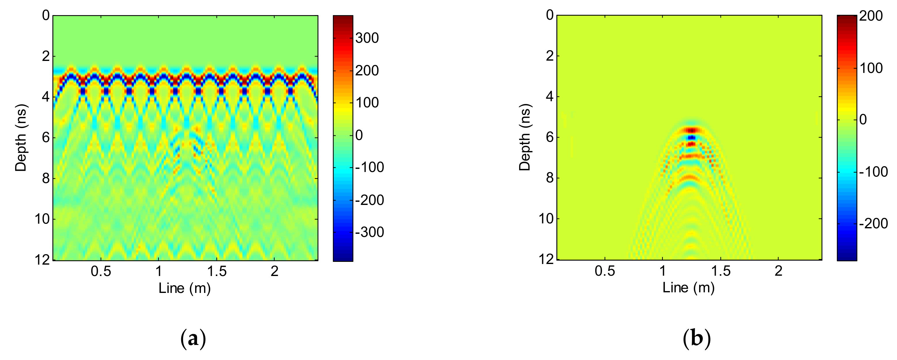
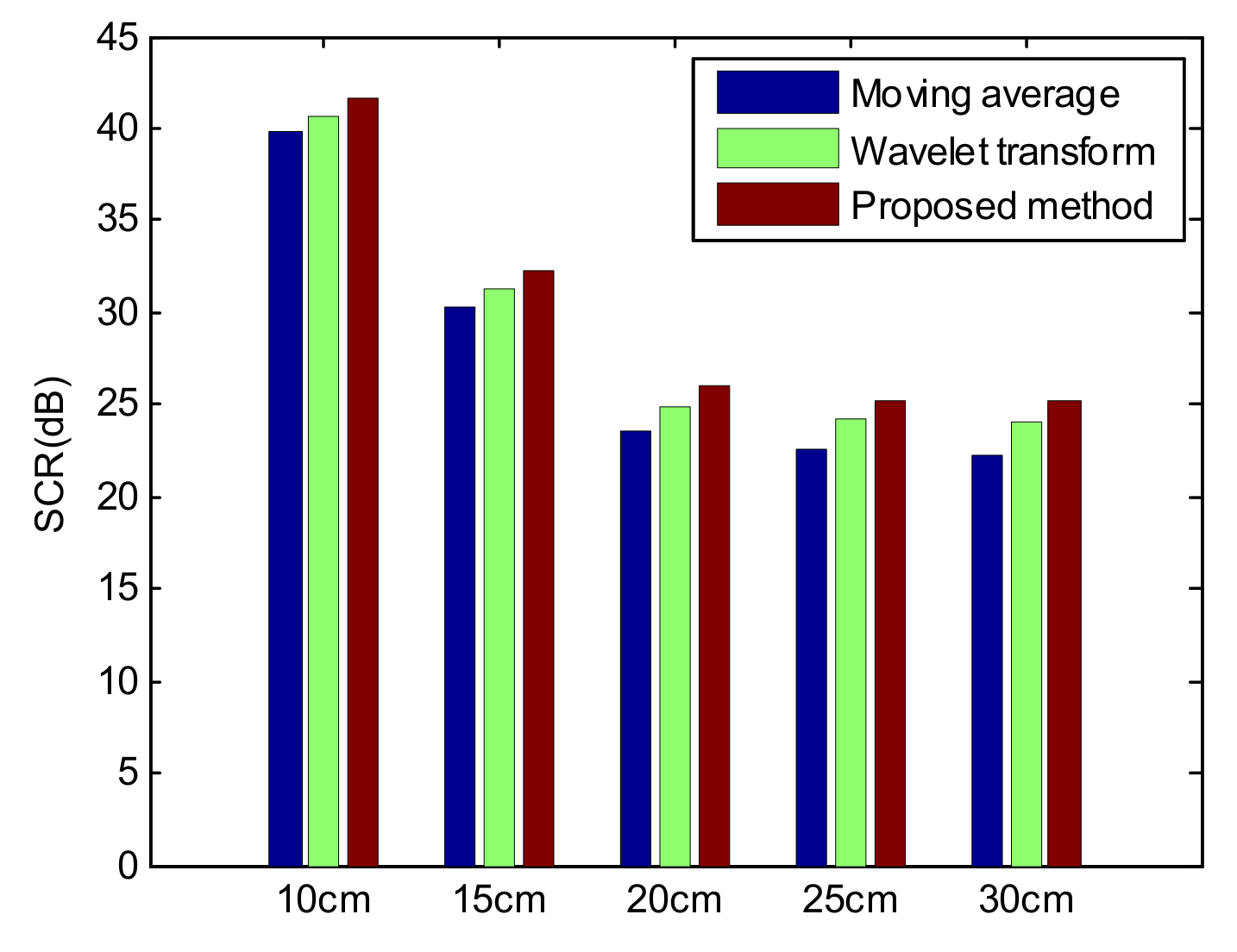
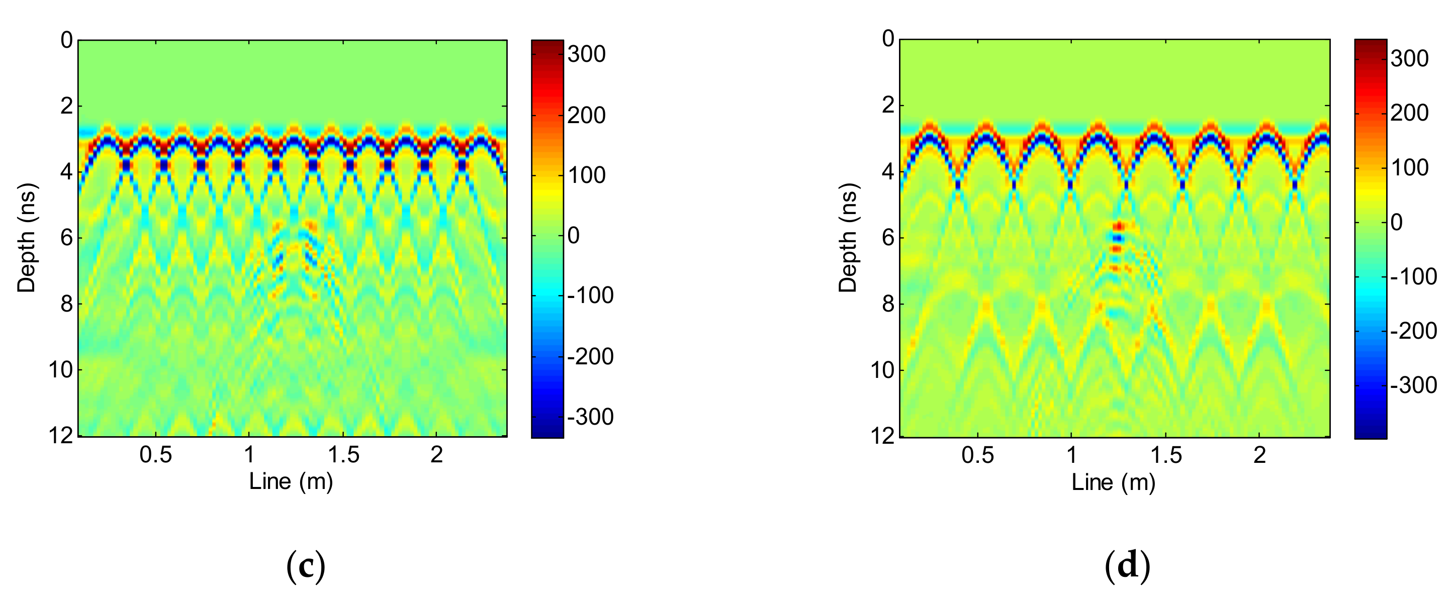
2.1. Clutter Suppression

The GPR data collected from tunnel linings contain clutter, noise, and target signals. Clutter is mainly composed of direct waves, measurement noise can be regarded as Gaussian white noise, and target signals are reflected waves from disease and rebar in tunnel linings. According to Fresnel reflection law, the energy of a direct wave is approximately 50 percent of the transmitted energy, while the energy of the disease is very weak and is usually submerged by clutter [31].

As the state equation is used to describe the dynamic change law of the state variable, the current value of the state variable is estimated through the value of the previous state and the latest measured data. A Kalman filter is exactly suitable for GPR data, which is non-stationary data. Thus, it is adopted to suppress clutter in this paper.

(1)

GPR data model

The collected GPR data from a measurement position is called A-scan data, and the collected data from along the measurement direction is generally called B-scan data. If we let ${\mathrm{y}}_m(i)$, $c_m(i)$, $s_m(i)$, and $n_m(i)$ denote A-scan data, clutter, target signals, and the measurement noise of the $m-\mathrm{th}$ measure position, respectively, then $i$ represents the sample point in the depth direction. In order to separate the target signals and clutter, two hypotheses, ${\mathrm{H}}_0$ (the target signal is present) and ${\mathrm{H}}_1$ (the target signal is not present), must be tested against each other, as follows:

$${\mathrm{H}}_0:\hspace{0.33em}{\mathrm{y}}_m(i)=c_m(i)+s_m(i)+n_m(i) \mathrm{and}$$

(1)

$${\mathrm{H}}_1:\hspace{0.33em}{\mathrm{y}}_m(i)=c_m(i)+n_m(i)$$

(2)

(2)

State equation and measurement equation under ${\mathrm{H}}_0$

According to the signal model of a Kalman filter, when the target signal $s_m(i)$ is contained in the A-scan data ${\mathrm{y}}_m(i)$, the state equation and measurement equation of the GPR data can be expressed as follows:

$$\left[\begin{array}{c}{c}_m(i)\\ s_m(i)\\ b_m(i)\end{array}\right]=A\left[\begin{array}{c}{c}_{m-1}(i)\\ s_{m-1}(i)\\ b_{m-1}(i)\end{array}\right]+\left[\begin{array}{c}e{1}_{m-1}(i)\\ e{2}_{m-1}(i)\\ e{3}_{m-1}(i)\end{array}\right],$$

(3)

$${\mathrm{y}}_m(i)=B\left[\begin{array}{c}{c}_m(i)\\ s_m(i)\\ b_m(i)\end{array}\right]+n_m(i),$$

(4)

$$A=\left[\begin{array}{ccc}1& 0& 0\\ 0& 1& 1\\ 0& 0& 1\end{array}\right], \mathrm{and}$$

(5)

$$B=\left[\begin{array}{ccc}1& 1& 0\end{array}\right],$$

(6)

where $c_m(i)$, $s_m(i)$, and $b_m(i)$ are considered as the state variables and the A-scan data ${\mathrm{y}}_m(i)$ is regarded as measured data. $A$ and $B$ denote the transition matrix between the state variables and the gain matrix between the state variables and the measured data, respectively. $b_m(i)$ denotes the change of the target signal and $e{1}_{m-1}(i)$, $e{2}_{m-1}(i)$, and $e{3}_{m-1}(i)$ denote process noise.

(3)

Kalman filtering under ${\mathrm{H}}_0$

The main steps of Kalman filtering under the hypotheses ${\mathrm{H}}_0$ are shown below. First, the iterative initial conditions of the Kalman filtering are set by the measured data and the initial conditions are defined as follows:

$$c_0^{″}(i)=\frac{1}{M}{\displaystyle \sum _{m=1}^M{\mathrm{y}}_m(i)},$$

(7)

$$s_0^{″}(i)=0,$$

(8)

$$b_0^{″}(i)=0, \mathrm{and}$$

(9)

$$P_0^{″}(i)=\left[\begin{array}{ccc}\frac{1}{M}{\displaystyle \sum _{m=1}^M{\left({\mathrm{y}}_m(i)-c_0(i)\right)}^2}& 0& 0\\ 0& 0& 0\\ 0& 0& 0\end{array}\right],$$

(10)

where $P_0^{″}(i)$ denotes the initial value of the covariance matrix of the state variable estimation.

Second, without considering the process noise and measurement noise, the estimated value of the state variables is calculated as:

$$\left[\begin{array}{c}{c}_m^{\prime }(i)\\ s_m^{\prime }(i)\\ b_m^{\prime }(i)\end{array}\right]=A\left[\begin{array}{c}{c}_{m-1}^{″}(i)\\ s_{m-1}^{″}(i)\\ b_{m-1}^{″}(i)\end{array}\right].$$

(11)

Then, in order to minimize the mean square value of the state variable estimation error, the estimated value of the state variable is corrected by a weighted estimated error of the measured data, as follows:

$$\begin{array}{l}\left[\begin{array}{c}{c}_m^{″}(i)\\ s_m^{″}(i)\\ b_m^{″}(i)\end{array}\right]=\left[\begin{array}{c}{c}_m^{\prime }(i)\\ s_m^{\prime }(i)\\ b_m^{\prime }(i)\end{array}\right]\\ \hspace{1em}\hspace{1em}\hspace{1em}\hspace{1em}+H_m(i)\left({\mathrm{y}}_m(i)-B\left[\begin{array}{c}{c}_m^{\prime }(i)\\ s_m^{\prime }(i)\\ b_m^{\prime }(i)\end{array}\right]\right)\end{array}$$

(12)

where $H_m(i)$ denotes the weighted matrix, $P_m(i)$ denotes the covariance matrix of the state variable estimation error, $R_n$ represents the power of the measurement noise, and $Q$ represents the covariance matrix of the process noise.

$$H_m(i)=P_m(i)B^{\mathrm{H}}{(B{P}_m(i)B^{\mathrm{H}}+R_n)}^{-1}\mathrm{and}$$

(13)

$$P_m(i)={AP}_{m-1}^{″}(i)A^{\mathrm{H}}+Q.$$

(14)

In addition, using the weighted matrix, the covariance matrix of the state variable estimation error is also corrected for the next iteration:

$$P_{m-1}^{″}(i)=(I-H_m(i)B)P_m(i).$$

(15)

Along with the progress of the Kalman filter iterations, the target signals will gradually be separated from the clutter. The processing chain for the Kalman filtering under hypothesis ${\mathrm{H}}_0$ is as shown in Figure 2. The number of iterations is set by the signal-to-clutter ratio (SCR), and the target signal separated in the $m\text{-}\mathrm{th}$ iteration is $s_m^{″}(i)$.

(4)

Clutter suppression using Kalman filtering

When the target signal $s_m(i)$ is not contained in the A-scan data ${\mathrm{y}}_m(i)$, the state equation and measurement equation of the GPR data can be rewritten as Equations (16) and (17), respectively. The processing chain for the Kalman filtering under hypothesis ${\mathrm{H}}_1$ is similar to that of hypothesis ${\mathrm{H}}_0$:

$$c_m(i)=c_{m-1}(i)+e{1}_{m-1}(i) \mathrm{and}$$

(16)

$${\mathrm{y}}_m(i)=c_m(i)+n_m(i).$$

(17)

According to the Kalman filtering model, both with and without a target signal, the conditional probability of the GPR data obeying each model at a specific location is calculated and the current model state is judged by the conditional probability, and then the clutter is suppressed by the corresponding Kalman filtering model.

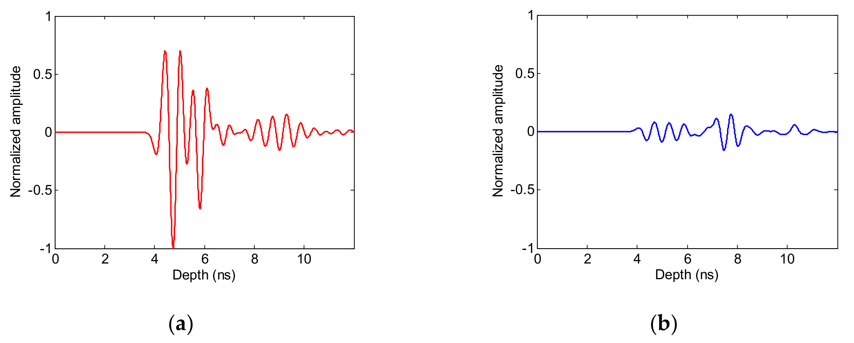
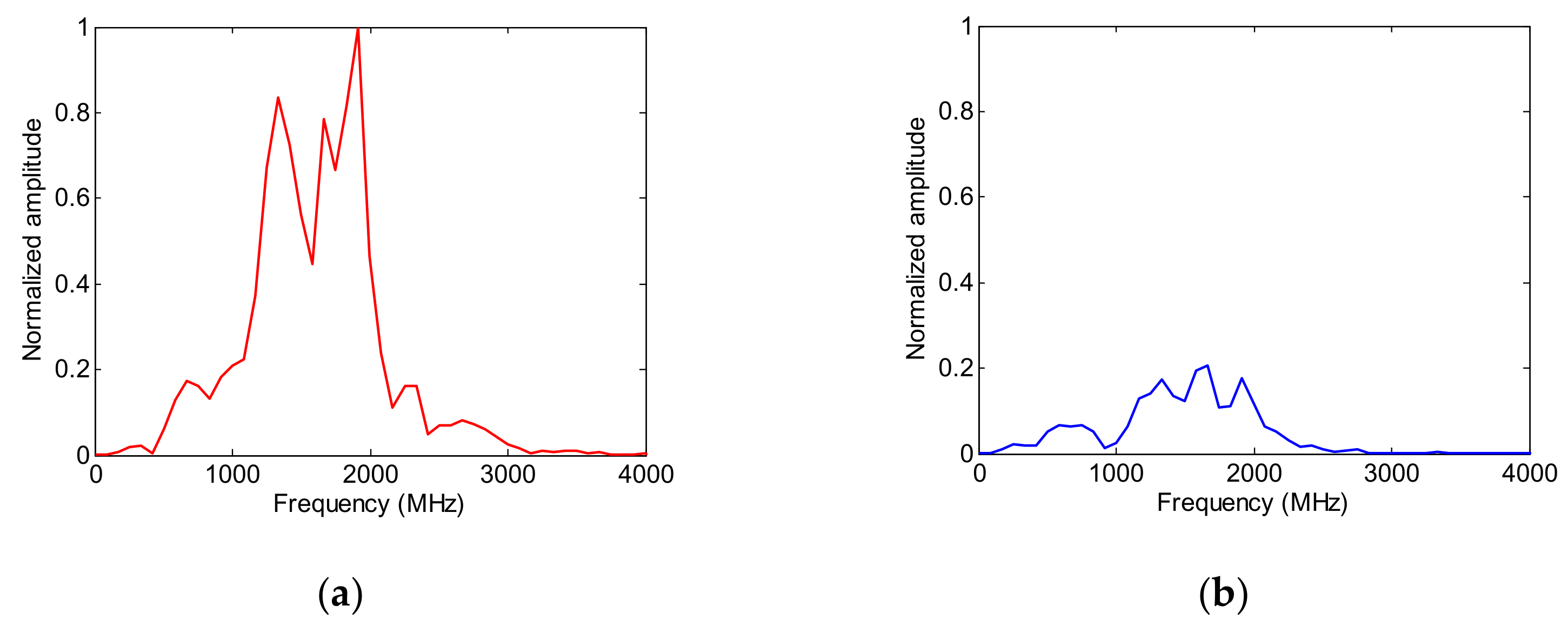
2.2. Rebar Interference Suppression

Due to the interference of strong reflection waves and multiple waves of rebar in tunnel linings, it is very difficult to identify the internal diseases of tunnel linings. Considering the great success of Unet in the field of image segmentation, this paper builds a network based on a convolution neural network which can complete the mapping from rebar interference data to non-rebar interference data so as to realize the suppression of rebar interference and the recovery of disease data, and then it improves the accuracy of disease detection.

In order to provide the data set needed for training the network, this paper first establishes a paired disease model, with and without rebar, whose other parameters are exactly the same. Then, GPRMAX software is used to simulate the paired disease model. The parameters of the simulation are shown in Section 3.1. The paired simulation results, shown in Figure 3 (taking the lack of density disease as an example), are used as the input data and output data of the network, respectively. Considering that deep learning requires a large amount of training data, 40,000 pairs of disease models are established in this paper. Among them are four types of common hidden diseases in tunnel linings–cavities, voids, lack of density, and cracks—with 10,000 pairs for each disease type.

In order to make the data sets of hidden diseases in tunnel linings more comprehensive, the locations, scales, and other parameters of the diseases are randomly distributed, and the distribution ranges refer to the slight levels of interim provisions for safety grade assessments of railway operation tunnel linings (railway transport letter [2004] No. 174). In addition, considering the influence of rebar depth, spacing, diameter, and other factors of disease data, the distribution of rebar in the disease data set must be diversified. Therefore, in the data set established in this paper, the depth, spacing, diameter, and other parameters of the rebar are also randomly distributed, and the distribution range is designed according to the railway tunnel design specifications.

In order to effectively suppress the rebar interference in the input data, this paper plans to add an attention module from the Unet structure, as shown in Figure 4. A Unet structure is divided into two symmetrical parts: the left half of the network is mainly used for feature extraction and the right half is up-sampled. Such a structure is also called an encoder–decoder structure.

The blue arrow in Figure 4 represents the convolution operation. The number of convolution kernels can be obtained by the number of layers of the feature image obtained. For example, 64-dimensional feature images can be obtained from the input B-scan image through 64 convolutional kernels, which are 1 × 1 in size. The red arrow represents the pooling operation. This paper uses the maximum pooling of 2 × 2, which can halve the lengths and widths of the input features. Through a series of convolution and pooling layers, the network changes an input B-scan image into a 1024-dimensional feature. This part of the network is an encoder structure.

The black arrow in Figure 4 represents the deconvolution operation of 2 × 2, which can double the lengths and widths of the input feature images. The green arrow is a copy operation. The yellow box obtained by copying the input features and the green box obtained by up-sampling are spliced to obtain a more “thick” feature in the third dimension, which can combine the shallow features containing more local details with the deep features containing more global information. Through a series of deconvolution layers and convolution layers, the 1024-dimensional features obtained in the middle are finally restored to a 1-dimensional output image. This part of the network is the decoder structure.

In addition, the black circle in Figure 4 represents the attention module and the purple arrow is the input of the attention module, while the structure of the attention module is shown in Figure 5. Before the shallow features are copied and stitched with the deep features after up-sampling, the shallow features x and deep features g are input into the attention module and the obtained attention coefficient a is multiplied with the shallow features x and stitched with the deep features after up-sampling.

In order to avoid the problem of network degradation in the process of network training, this paper adds a residual block, as shown in Figure 6, and it trains the Unet, attention Unet, and attention Unet with the residual block using the disease data set at the same time. The superiority of the proposed network is verified by the suppression of the rebar interference.

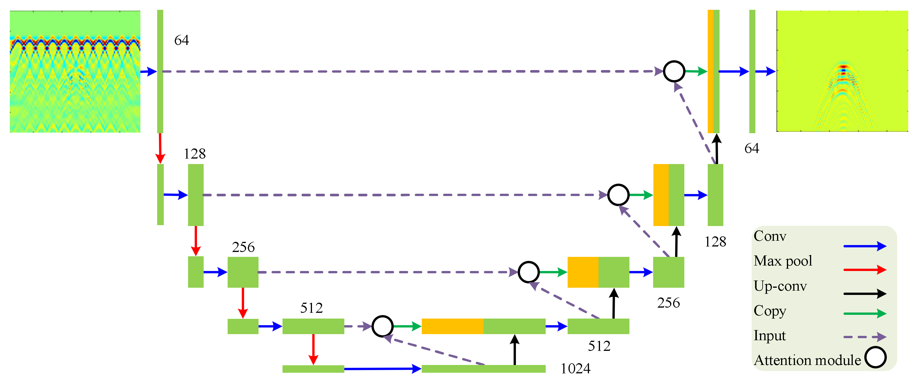
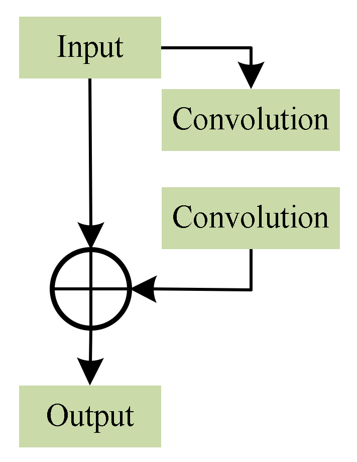
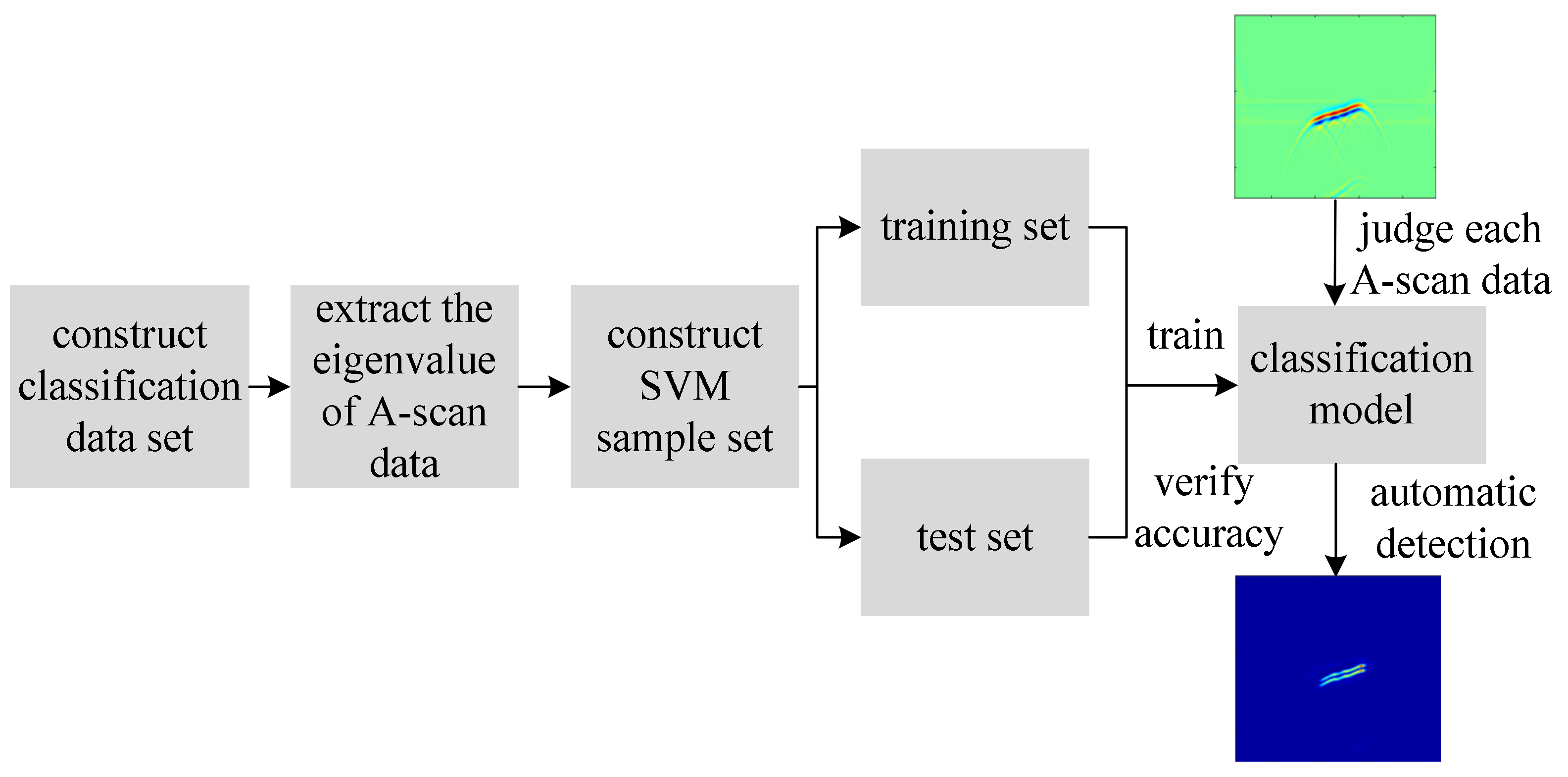
2.3. Automatic Disease Detection

The one-dimensional A-scan data collected by radar in a single measurement position contains rich time-frequency information which can reflect the essential characteristics of hidden diseases, and it has a low amount of data. The two-dimensional B-scan data collected by radar along the measurement direction can reflect the shape information of hidden diseases in tunnel lining. Considering the large amount of data in the process of detecting hidden diseases in tunnel linings, this paper extracts the multi-dimensional features of A-scan data, and then it uses an SVM (support vector machine) algorithm to build a binary classification model and it classifies the A-scan data from the computer vision, judges whether or not it contains disease signals, and completes the rapid automatic detection of disease.

The processing chain of automatic disease detection is shown in Figure 7. As the SVM algorithm is based on the training of positive and negative samples to complete the disease detection, this paper randomly extracts 120 A-scan data without rebar interference from the data set built in Section 2.2 to form a classification data set in which the first 60 are non-disease data and the last 60 are disease data. Among the disease data are four types of common hidden diseases in tunnel linings: cavities, voids, lack of density, and cracks.

Then, six identification features of each A-scan datum in the classification data set are calculated. The six identification features are the maximum amplitude, maximum amplitude occurrence time, energy, spectrum variance, time-frequency information entropy, and the maximum amplitude of the first intrinsic mode function (IMF). The SVM sample set (with a sample dimension of 6 and a sample number of 120) is established by taking the identification features of 120 A-scan data in the classification data set. The identification features of non-disease data are negative samples, and the label is 0. The identification features of the disease data are positive samples, and the label is 1.

Finally, after normalizing the SVM sample set, 30 positive and 30 negative samples are extracted to form the training set, and the remaining samples form the test set. The SVM is used to train the training set to obtain the binary classification model, and the test set is used to verify the classification accuracy of the model. The model can automatically detect whether A-scan data, after interference suppression, contain disease information.

3. Experimental Results

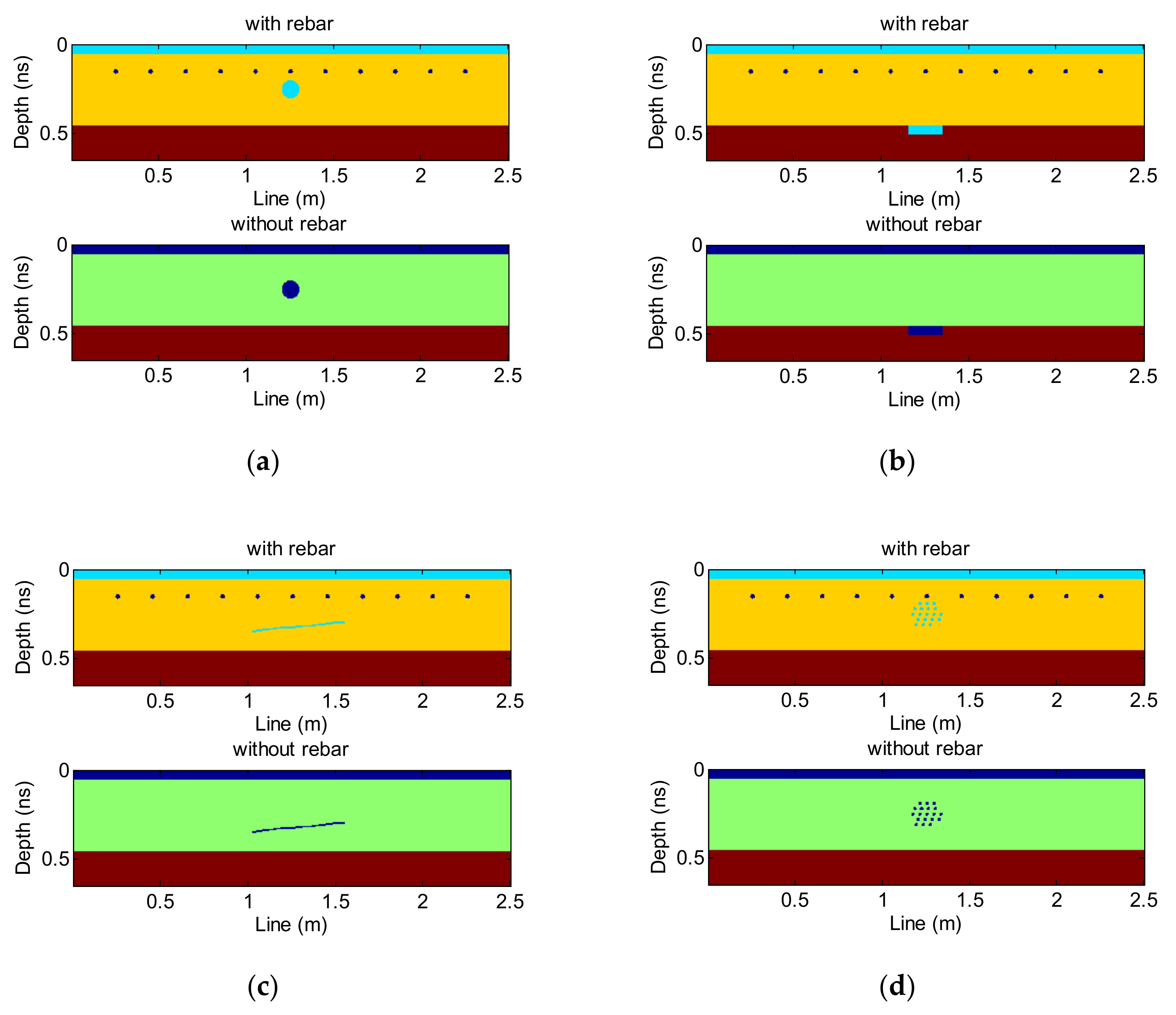
3.1. Establishing a Paired Disease Data Set

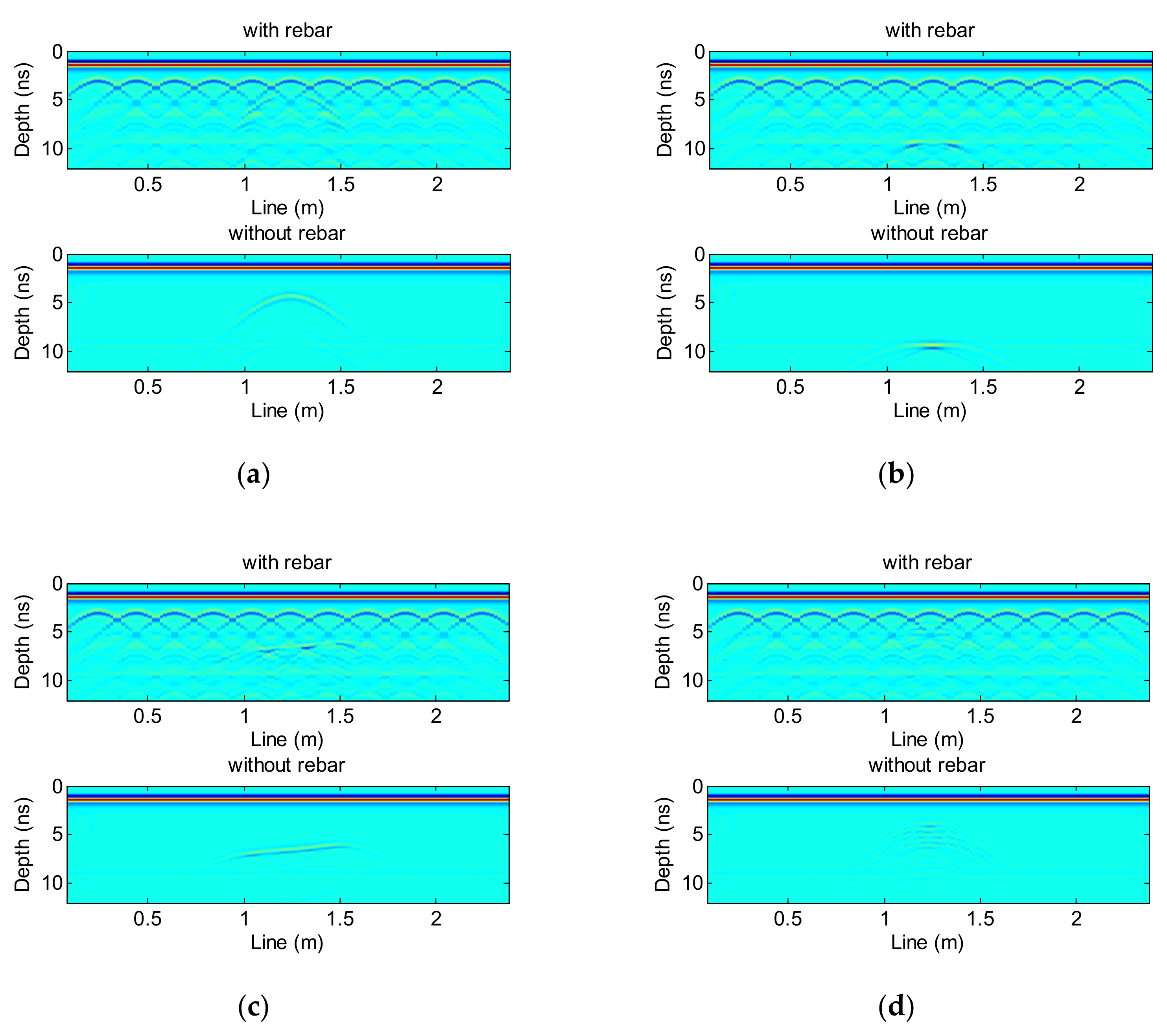
In this paper, GPRMAX software [32] is used to simulate hidden disease in tunnel lining. Considering the cost of the calculation time, the model size is set as 2.5 m (line direction) × 0.65 m (depth direction). The radar antenna scans from left to right on the upper boundary of the model. The center frequency of the radar antenna is 900 MHz, the input signal source is a Ricker wavelet, and the antenna is air-coupled. The time window is 12 ns, the radar antenna scans from left to right on the upper boundary of the model (moving 2 cm each time), and 115 signals are collected.

Considering that deep learning requires a large amount of training data, 40,000 pairs of diseases are simulated. Among them are four types of common hidden diseases in tunnel linings—cavities, voids, lack of density, and cracks—with 10,000 pairs of each type used. Figure 8 shows an example model for each of the four diseases, and the corresponding simulation results are shown in Figure 9.

3.2. Results

Figure 10 shows the clutter suppression results for each of the four diseases using the proposed clutter suppression method. Obviously, the clutter is largely suppressed. In order to further analyze the advantages of the proposed method, a comparative experiment is carried out. Taking a void disease as an example, the disease has different burial depths. Figure 11 presents the signal-to-clutter ratio (SCR) at various burial depths and for different clutter suppression methods (moving average [33], wavelet transform [34], and the proposed method). It is clearly seen that the proposed method is superior to the other methods.

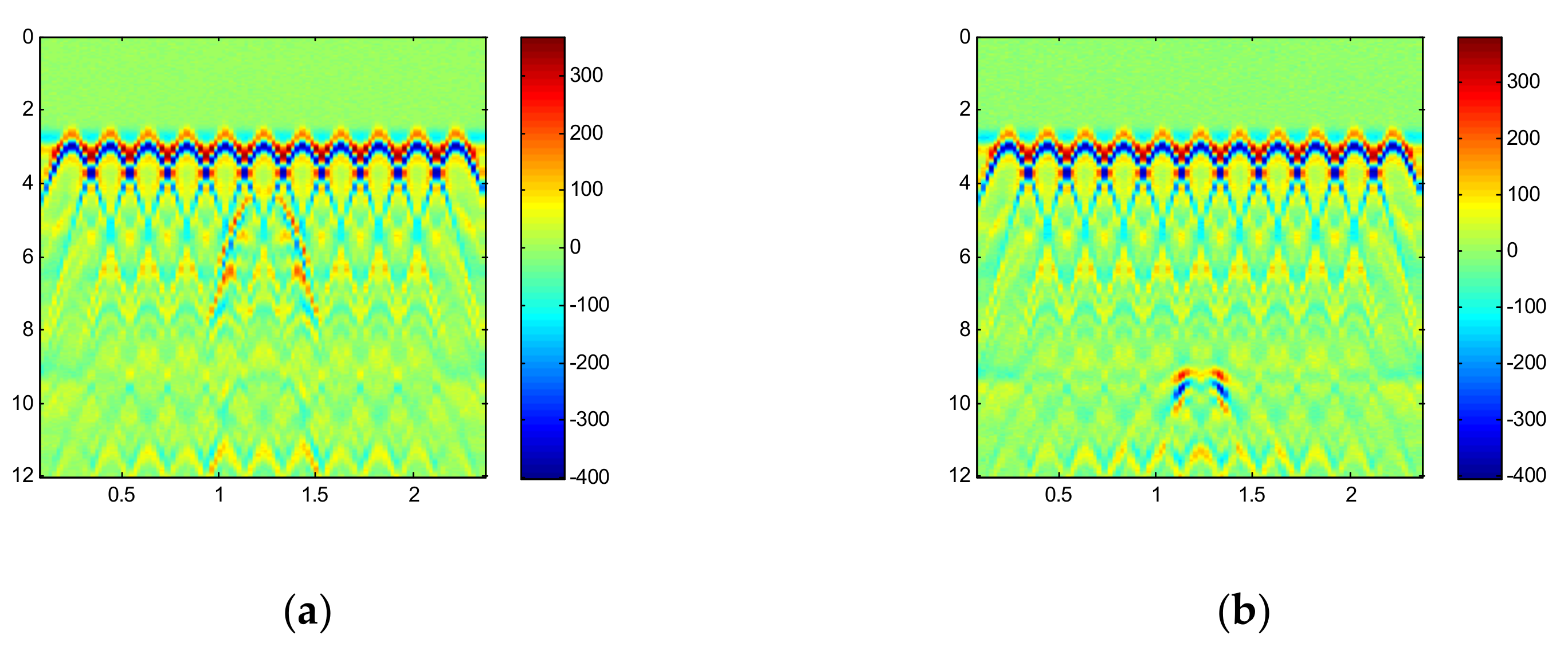
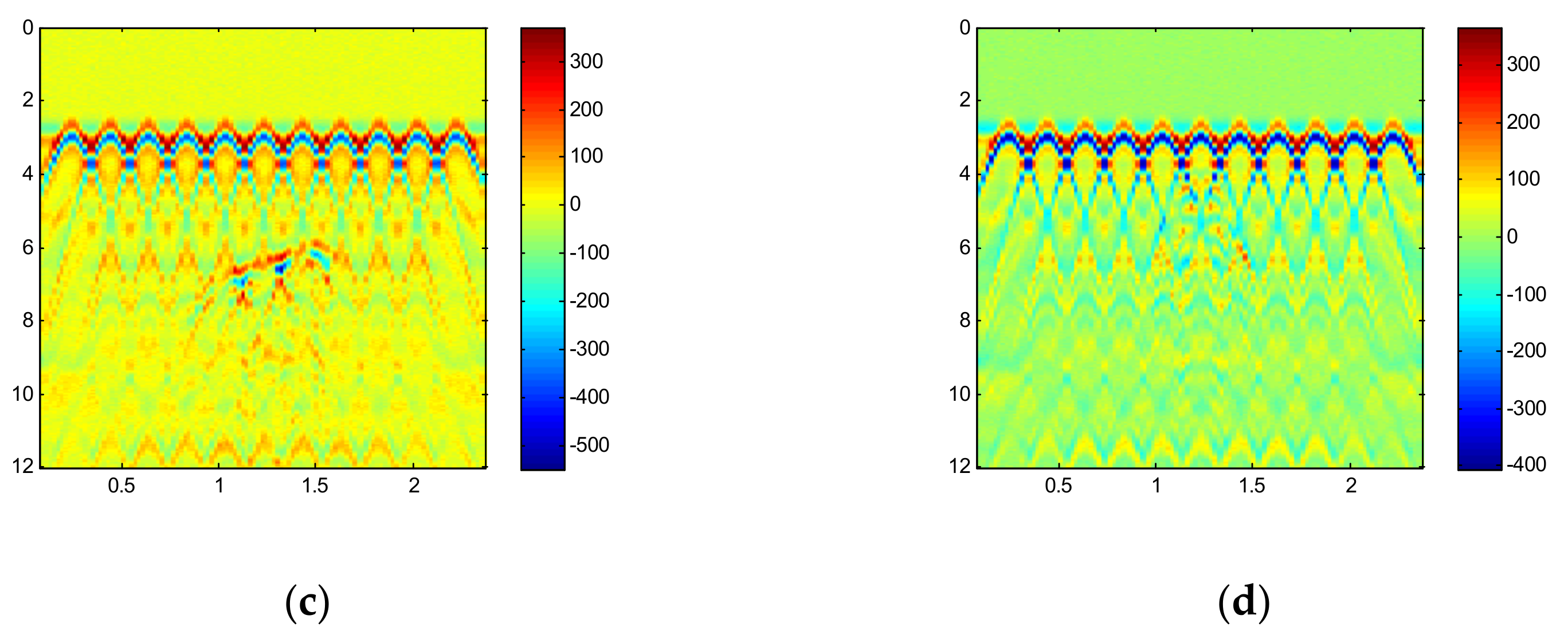
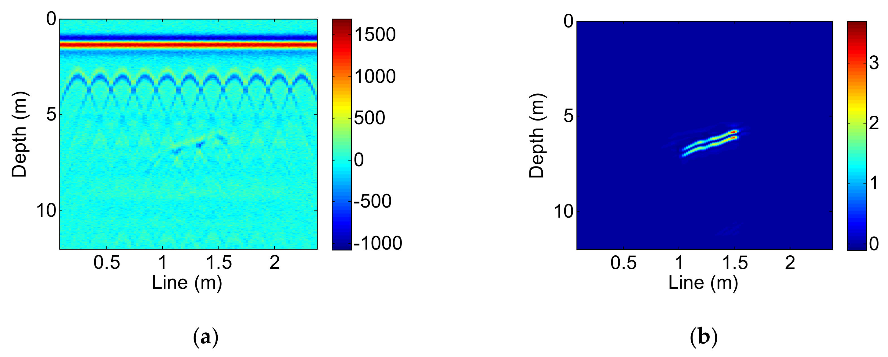
3.3. Rebar Interference Suppression Results

Taking lack of density as an example, the disease is disturbed by rebar with various depths, spacing, and radii, and the corresponding simulation results are shown in Figure 12. The input data of the network is trained by the paired disease data set from Section 3.1, as shown in Figure 12. Figure 13 presents the corresponding output results of the trained network. Obviously, the factors of depth, spacing, and radius have almost no effect on the rebar suppression effects of the network designed in this paper, and thus the network can remove the rebar interference and recover the disease signal effectively.

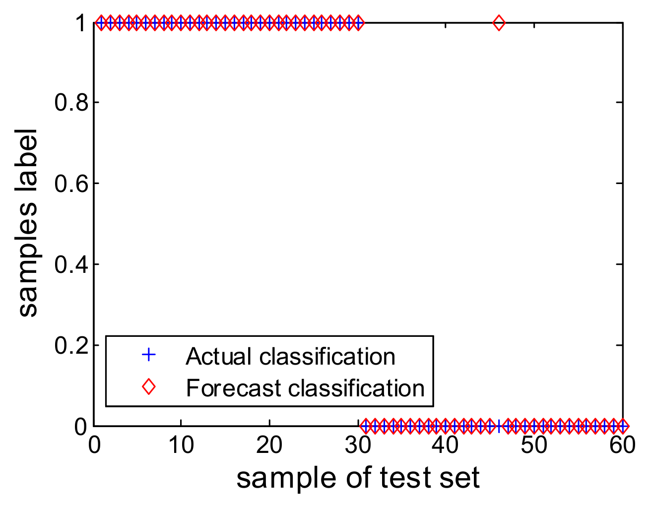
3.4. Disease Automatic Detection Results

This section extracts multi-dimensional features of the diseases in the time domain, frequency domain, and time-frequency domain to solve the problem of single judgment basis in disease detection.

Taking lack of density as an example, we select one disease’s A-scan data and one non-disease’s A-scan data, as shown in Figure 14. After the clutter and rebar interference are suppressed, the disease data is mainly composed of reflected waves in the disease area, while the non-disease data does not contain any, or does contain only a small number of, diffraction waves in the disease area. Because the two-way travel time of a diffraction wave is greater than that of a reflection wave, the maximum amplitude of the non-disease data is less than that of the disease data, and the maximum amplitude appears later than that of the disease data. In addition, considering that there are peaks caused by noise interference in the data, this paper selects the maximum amplitude, maximum amplitude occurrence time, and energy as the identification features of the disease in the time domain.

As the attenuation of high-frequency electromagnetic waves in concrete medium is faster than that of low-frequency electromagnetic waves, the proportion of low-frequency components of non-disease data increases and the distribution is relatively scattered. The spectrum variance can reflect this regularity, and so this paper uses the spectrum variance as the identification feature of the disease in the frequency domain. Figure 15 shows the spectrum of Figure 14, with the amplitude of each frequency component in the spectrum of the non-disease data reduced, which is consistent with the time domain analysis.

The difference in the energy distribution between the disease data and the non-disease data can be described by time-frequency information entropy in the time-frequency domain. In addition, the first IMF of the empirical mode decomposition (EMD) can better reflect the disease information. Therefore, this paper uses time-frequency information entropy and the maximum amplitude of the first IMF as the identification features of the disease in the time-frequency domain.

Using the above six identification features, the training set and test set are established according to Section 2.3. An SVM algorithm is used to train the samples of the training set to obtain the binary classification model. The accuracy of the classification model is verified by the test set, and the results are as shown in Figure 16. There are 60 samples in the test set, of which 1–30 are positive samples without disease and 31–60 are negative samples with disease. Only one non-disease signal corresponding to sample 46 is misjudged as a disease signal, and the model’s accuracy is approximately 98.3%.

Taking a crack as an example, the distribution range of the disease along the measurement direction is 1.02 m to 1.55 m, corresponding to forty-five to seventy-two of the A-scan data. The trained model is used to detect the disease from the radar data by judging (one by one) whether each A-scan data set contains a disease signal, and the results after clutter and rebar interference suppression and automatic disease detection are shown in Figure 17. The disease area is consistent with the actual location of the disease, and thus the automatic detection method of disease proposed in this paper is proved.

4. Conclusions

This paper introduces a novel method for the automatic detection of diseases in tunnel linings utilizing ground-penetrating radar. Firstly, a Kalman filter and a convolution neural network are adopted to solve the influence of clutter and the strong reflection of rebar on disease detection. Then, an SVM is used to realize the intelligent classification of disease data, which solves the problems of radar detection of lining disease being mainly manual and detection accuracy depending too much on the experience level of technicians, along with the poor degree of automation. In addition, the signal features are extracted in the time domain, frequency domain, and time-frequency domain, and six identification features of the maximum amplitude, maximum amplitude occurrence time, energy, spectrum variance, time-frequency information entropy, and maximum amplitude of the first intrinsic mode function (IMF) are obtained, which solves the problem of the single basis for disease interpretation and judgment, and thus affects the accuracy of disease detection.

References

1. Liu, X.R.; Shu, Z.L.; Zhu, C.H. Study of forward simulation for ground penetration radar three-dimensional detection of tunnel. Chin. J. Rock Mech. Eng. 2010, 29, 2221–2228. [Google Scholar]
2. Shu, Z.L.; Liu, X.R.; Zhu, C.H. Study of model test about 3D GPR detection of tunnel lining cavity. Rock Soil Mech. 2011, 32, 551–558. [Google Scholar]
3. Xu, H.; Liu, J.P.; Fan, C.Y. Forward modeling of tunnel lining diseases ground penetrating radar wave field and characteristics analysis. J. Cent. South Univ. (Sci. Technol.) 2013, 44, 4581–4587. [Google Scholar]
4. Dong, Y.; Wang, J.; Wang, Z.; Zhang, X.; Gao, Y.; Sui, Q.; Jiang, P. A deep-learning based multiple defect detection method for tunnel lining damages. IEEE Access 2019, 7, 182643–182657. [Google Scholar] [CrossRef]
5. Yan, T.; Yang, J.; Liu, Z.; Peng, A. Application of instantaneous amplitude gradient for ground penetrating radar signal analyses. Arab. J. Geosci. 2018, 11, 1–10. [Google Scholar] [CrossRef]
6. Benedetto, F.; Tosti, F. A signal processing methodology for assessing the performance of ASTM standard test methods for GPR systems. Signal Process. 2017, 132, 327–337. [Google Scholar] [CrossRef]
7. Li, Y.; Li, S.C.; Xu, L.; Liu, B.; Lin, C.J.; Zhang, F.K.; Yang, L. Forward simulation of ground penetrating radar and its application to detection of tunnel lining diseases. Rock Soil Mech. 2016, 37, 1001–1008. [Google Scholar]
8. Ji, H.; Yin, B.; Zhang, J.; Zhang, Y. Joint Inversion of Evaporation Duct Based on Radar Sea Clutter and Target Echo Using Deep Learning. Electronics 2022, 11, 2157. [Google Scholar] [CrossRef]
9. Chen, X.; Guan, J.; Bao, Z.; He, Y. Detection and Extraction of Target with Micro-Motion in Spiky Sea Clutter via Short-time Fractional Fourier Transform. IEEE Trans. Geosci. Remote Sens. 2014, 52, 1002–1018. [Google Scholar] [CrossRef]
10. Cheikh, K.; Soltani, F. Application of Neural Networks to Radar Signal Detection in K-distributed Clutter. IEEE Proc. Radar. Sonar. Navig. 2006, 153, 460–466. [Google Scholar] [CrossRef]
11. Chang, J.; Fu, X.; Zhao, C.; Lang, P.; Feng, C. Distributed Radar Target Detection Based on RF-SSA in Non-Gaussian Noise. Electronics 2022, 11, 2319. [Google Scholar] [CrossRef]
12. Bao, Q.Z.; Li, Q.C.; Chen, W.C. GPR data noise attenuation on the Curvelet transform. Appl. Geophys. 2014, 11, 301–310. [Google Scholar] [CrossRef]
13. Wang, X.; Liu, S. Noise suppressing ang direct wave arrivals removal in GPR data based on Shearlet transform. Signal Process. 2017, 132, 227–242. [Google Scholar] [CrossRef]
14. Yao, Q.; Chun-lin, H.; Min, L.; Wei, X. Adaptive clutter reduction based on wavelet transform and principal component analysis for ground penetrating radar. J. Radars 2015, 4, 445–451. [Google Scholar]
15. Zhou, X.; Chen, H.; Li, J. An automatic GPR B-Scan image interpreting model. IEEE Trans. Geosci. Remote 2018, 56, 3398–3412. [Google Scholar] [CrossRef]
16. Lei, W.; Hou, F.; Xi, J.; Tan, Q.; Xu, M.; Jiang, X.; Liu, G.; Gu, Q. Automatic hyperbola detection and fitting in GPR B-scan image. Autom. Constr. 2019, 106, 1–11. [Google Scholar] [CrossRef]
17. Núñez-Nieto, X.; Solla, M.; Gómez-Pérez, P.; Lorenzo, H. GPR signal characterization for automated landmine and UXO detection based on machine learning techniques. Remote Sens. 2014, 6, 9729–9748. [Google Scholar] [CrossRef] [Green Version]
18. Kaur, P.; Dana, K.J.; Romero, F.A.; Gucunski, N. Automated GPR rebar analysis for robotic bridge deck evaluation. IEEE Trans. Cybern. 2016, 46, 2265–2276. [Google Scholar] [CrossRef]
19. Mahallawy, M.; Hashim, M. Material Classification of underground utilities from GPR images using DCT-based SVM approach. IEEE Geosci. Remote Sens. Lett. 2013, 10, 1542–1546. [Google Scholar] [CrossRef]
20. Jiang, W.; Ren, Y.; Liu, Y.; Leng, J. Artificial Neural Networks and Deep Learning Techniques Applied to Radar Target Detection: A Review. Electronics 2022, 11, 156. [Google Scholar] [CrossRef]
21. Bhatia, J.; Dayal, A.; Jha, A.; Vishvakarma, S.K.; Joshi, S.; Srinivas, M.B.; Yalavarthy, P.K.; Kumar, A.; Lalitha, V.; Koorapati, S.; et al. Classification of Targets Using Statistical Features from Range FFT of mmWave FMCW Radars. Electronics 2021, 10, 1965. [Google Scholar] [CrossRef]
22. Travassos, X.L.; Avila, S.L.; Ida, N. Artificial Neural Networks and Machine Learning techniques applied to Ground Penetrating Radar: A review. Appl. Comput. Inf. 2018, 17, 296–308. [Google Scholar] [CrossRef]
23. Gao, J.; Lu, Y.; Qi, J.; Shen, L. A Radar Signal Recognition System Based on Non-Negative Matrix Factorization Network and Improved Artificial Bee Colony Algorithm. IEEE Access 2019, 7, 117612–117626. [Google Scholar] [CrossRef]
24. Liao, K.; Si, J.; Zhu, F.; He, X. Radar HRRP Target Recognition Based on Concatenated Deep Neural Networks. IEEE Access 2018, 6, 29211–29218. [Google Scholar] [CrossRef]
25. Chen, X.; Guan, J.; Huang, Y.; Liu, N.; He, Y. Radon-linear Canonical Ambiguity Function-based Detection and Estimation Method for Marine Target with Micromotion. IEEE Trans. Geosci. Remote Sens. 2015, 53, 2225–2240. [Google Scholar] [CrossRef]
26. Liu, T.; Su, Y.; Huang, C. Inversion of ground penetrating radar data based on neural networks. Remote Sens. 2018, 10, 730–738. [Google Scholar] [CrossRef] [Green Version]
27. Tbarki, K. Adaptive landmine detection and localization system based on incremental one-class classification. J. Appl. Remote Sens. 2018, 12, 1–22. [Google Scholar] [CrossRef]
28. Tong, Z.; Gao, J.; Yuan, D. Advances of deep learning applications in ground-penetrating radar: A survey. Constr. Build. Mater. 2020, 258, 1–13. [Google Scholar] [CrossRef]
29. Shahsavar, S.; Fakoor, M.; Berto, F. Mixed mode I/II fracture criterion to anticipate cracked composite materials based on a reinforced kinked crack along maximum shear stress path. Steel Compos. Struct. 2021, 39, 765–779. [Google Scholar]
30. Erfani, S.; Vakili, A.; Akrami, V. Numerical investigation on the flexural links of eccentrically braced frames with web openings. Steel Compos. Struct. 2021, 39, 171–188. [Google Scholar]
31. Wang, S.; Li, L.; Cheng, S.; Yang, J.; Jin, H.; Gao, S.; Wen, T. Study on an improved real-time monitoring and fusion prewarning method of water inrush in tunnels. Tunn. Undergr. Space Technol. 2021, 112, 103884. [Google Scholar] [CrossRef]
32. Giannopoulos, A. Modelling ground penetrating radar by GprMax. Constr. Build. Mater. 2005, 19, 755–762. [Google Scholar] [CrossRef]
33. Zoubir, A.M.; Chant, I.J.; Brown, C.L.; Barkat, B.; Abeynayake, C. Signal processing techniques for landmine detection using impulse ground penetrating radar. IEEE Sens. J. 2002, 2, 41–51. [Google Scholar] [CrossRef] [Green Version]
34. Carevic, D. Clutter reduction and target detection in Ground Penetrating Radar data using wavelets. Proc. SPIE 1999, 3710, 973–978. [Google Scholar] [CrossRef]
Figure 1. Tunnel structure damage. (a) Split lining. (b) Lining block.
Electronics 11 03290 g001
Figure 2. Processing chain for the Kalman filtering under hypothesis H 0 .
Electronics 11 03290 g002
Figure 3. The paired simulation results of the diseases: (a) with rebar, and (b) without rebar.
Electronics 11 03290 g003
Figure 4. Added attention module from the Unet structure.
Electronics 11 03290 g004
Figure 5. The structure of the attention module.
Electronics 11 03290 g005
Figure 6. The structure of the residual block.
Electronics 11 03290 g006
Figure 7. The processing chain of automatic disease detection.
Electronics 11 03290 g007
Figure 8. Hidden disease model: (a) void, (b) cavity, (c) crack, and (d) lack of density.
Electronics 11 03290 g008
Figure 9. Hidden disease simulation results: (a) void, (b) cavity, (c) crack, and (d) lack of density.
Electronics 11 03290 g009
Figure 10. Clutter suppression results: (a) void, (b) cavity, (c) crack, and (d) lack of density.
Electronics 11 03290 g010aElectronics 11 03290 g010b
Figure 11. SCR at various burial depths and for different clutter suppression methods.
Electronics 11 03290 g011
Figure 12. Input data of the trained network (unit: cm). (a) Depth of 10, spacing of 20, and radius of 1.25. (b) Depth of 15, spacing of 20, and radius of 1.25. (c) Depth of 10, spacing of 20, and radius of 1. (d) Depth of 10, spacing of 30, and radius of 1.25.
Electronics 11 03290 g012aElectronics 11 03290 g012b
Figure 13. Output results of the trained network. (a) Depth of 10, spacing of 20, and radius of 1.25. (b) Depth of 15, spacing of 20, and radius of 1.25. (c) Depth of 10, spacing of 20, and radius of 1. (d) Depth of 10, spacing of 30, and radius of 1.25.
Electronics 11 03290 g013
Figure 14. A-scan data: (a) disease data, and (b) non-disease data.
Electronics 11 03290 g014
Figure 15. Spectrum of A-scan data: (a) disease data, and (b) non-disease data.
Electronics 11 03290 g015
Figure 16. The accuracy of the classification model.
Electronics 11 03290 g016
Figure 17. Disease detection results: (a) before detection, and (b) detection results.
Electronics 11 03290 g017
Publisher’s Note: MDPI stays neutral with regard to jurisdictional claims in published maps and institutional affiliations.