1. Introduction
Digital twins, a concept from the industrial internet of things (IIoT), is the discipline of devising highly capable simulation models, especially those that consume data from streaming for improving performance. Devising a simulation model of clinical behavior in front of a disease is a task that is much more difficult than those for manufacturing processes, because humans are so unpredictable and engineering approaches obviously do not apply. The use of digital twins in healthcare systems is currently a hot topic under research [
1]. In particular, the authors of [
2] design a behavioral healthcare model for the case of lung cancer patients, which can be fed up into a decision support system [
3].
Data-based solutions in the healthcare domain lead to privacy concerns [
4]. Anonymization arises as a tool to mitigate risks when gathering and massively processing personal healthcare data [
5]. However, data anonymization is usually seen as a major problem in data analytics because it could lead to information loss [
6], reducing the knowledge contained in the dataset [
7].
Nevertheless, new training procedures, such as generative adversarial networks (GANs), aim at learning representations that preserve the most relevant part of the information. As a result of the GAN-based anonymization phase, a seedbed can be obtained from the training data that allows not only to capture information from the original data avoiding privacy concerns but also to generate new synthetic information with a similar behavior to the original one [
8]. Moreover, it is worth noting that obtaining clinical data has a high cost and, many times, information is very limited. By developing reliable methods for data augmentation with synthetic instances, medical professionals can benefit from this valuable information [
9]. For instance, computed tomography (CT) images of the pelvis are synthetically generated in [
10] for patients with cervical cancer using a conditional generative adversarial network based on a shallow U-Net (sU-Net) with an encoder/decoder depth of 2. Digital pathology and histopathological image processing are other domains where GANs are being extensively explored in medical advanced imaging [
11,
12]
The validation of synthetic samples, checking that they follow a distribution similar to that of real patients, is a challenge [
13,
14]. As a simple solution, generated synthetic data are mainly validated from the machine learning perspective using loss functions, which are those selected for model optimization. As far as the model is optimized during training, the selected loss function is minimized. Hence, the better a model is in terms of the workload of interest, the better the generated synthetic data [
15]. It is well known that this implication is not always true; hence, some research is taking a different direction [
16].
Performance evaluation using metrics, such as mean square error, for instance, is very complicated to be employed when information is in the form of images or graphs—in fact, in any domain that is not a metric space. For this reason, metric is usually replaced by subjective ‘expert decision’, oncologists in this case [
17,
18].
In this paper, we offer a different perspective to design an objective validation tool, which is very reasonable in decision making, applying to most of the cases in healthcare. This approach is statistical decision making—that is, to rely in hypothesis testing: is the model good enough to use? Does the model pass rigorous hypothesis testing criteria? This approach is closely related with the resemblance evaluation, especially the univariate resemblance analysis proposed in [
19] when defining standardized metrics for synthetic tabular data evaluation. However, beyond the proposal of a metric, we show for the case at hand how loss minimization and hypothesis validation are not always well aligned. Hence, statistical decision making should be considered along with model optimization’s losses, enforced metrics or expert assessment for validation in domains such as synthetic data generation in the healthcare domain.
The rest of this paper is structured as follows: In the next section, the available database with lung cancer patients records is introduced; the methods used, the treatment of missing values, and pre- and post-processing steps are described. Furthermore, a short introduction about generative adversarial networks is also provided. Experimentation and results are presented in
Section 3, and they are validated by using the statistical criterion of goodness of fit tests. Finally, a conclusion and discussion are provided about the work developed and the results obtained.
2. Materials and Methods
In this section, the available real-world database is presented and analyzed. First, the method used to clean and pre-process this database before being used in the proposed GAN structure for synthetic data generation is described. Next, a post-processing of the synthetic data is developed in order to obtain similar data to the real data.
2.1. Database of Lung Cancer Patients
This study is carried out using data from clinical trials of diagnosed lung cancer patients once ethical approval was obtained from the associated legal body. Clinical data come from patients in the Hospital Universitario Virgen del Rocío (HUVR), which is located in Seville, Spain. This multi-center hospital complex belongs to the Andalusian Public Health System, with more than 8400 professionals under its charge and with an annual budget of more than five hundred million euros. It is a third-level hospital whose area of influence is Western Andalusia and has a staff of 1279 installed beds. The database is maintained and managed using the platform
OpenClinica [
20], which collected the information of the diagnosed lung cancer patients. In order to preserve the privacy of the patients, the dataset has been anonymized from the original database. The health team validated the anonymized dataset before any study.
Let us indicate that the considered features in the database are provided as different types: that is, nominal, ordinal and quantitative features. This fact is very important in order to elaborate an adequate data trial for the GANs because these deal with neural networks which are fed with quantitative features. Thus, all the nominal and ordinal data must be converted to numerical data in a pre-processing step. Nevertheless, nominal variables cannot be codified as quantitative features as far as no prior order is defined in them. Therefore, we hypothesize that our model will handle this type of data properly and will provide us with acceptable results [
21]. The validation phase will confirm our hypothesis with respect to the nominal features.
It is worth noting that in the original dataset, outliers were previously treated for the health and statistical team in the hospital. The obtained dataset was normalized in the range from 0 to 255 in order to be converted in a pixels image. This is in our interest because we want to unify all kinds of data in the form of healthcare images. In this form, data can naturally be fed to the GAN structure, as it usually works on images. Tthis form of data visualization makes the job of the medical team—understanding the information obtained from the GAN structure—easier.
The dataset under consideration, which is recorded in CSV (comma-separated values) format, contains the information about 886 lung cancer patients and 64 features. The features are related to one of the following categories: Medical record, Evolution and clinical course, Dosimetry, and Quality of life. A deep and detailed analysis of the dataset and its features can be found in [
2].
An important characteristic in the dataset is missing values. Since instances in the dataset are translated into an image for each patient, these missing values are not a relevant problem. Nevertheless, it is a crucial problem when a model of machine learning is sought because the performance of these models is usually sensible to missing values.
2.2. Missing Values
The number of values of the dataset is 56,704 (), of which 6172 are missing, that is, a percentage of . These missing values are represented by the value ’0’ in the original dataset.
Since the main objective in this research is to replicate and validate original health data, that is, the model to be built must replicate data in a realistic way, we consider that even missing values must be replicated, because they are usually present in electronic health registers. Nevertheless, the number of missing values is too large for some instances in order to obtain a good performance from a machine learning perspective. Therefore, a study of these missing values must be carried out to eliminate those instances that are expected to downgrade the model performance, but not all of them, because we want to replicate usual registers.
In this point, two questions will be answered, and the associated decisions will be made:
At this point, it is worth noting that when the medical team fills the items in the Openclinica software platform, they do not follow any standardized protocol. Hence, it can be considered that the imputation of one feature or another depends on the dedication of the doctor and the status of the patient. Therefore, if the number of missing values is high, it indicates that either the patient’s clinical history or the annotated feature is not much more relevant than the others. It is true that other motivations exist: for example, it may be that the variable has been recently considered in the software platform and not all patients have a record of it or there is new research that indicates that a feature little considered previously now is more relevant.
2.3. Pre-Processing Data
It is well known that inputs in GANs must be normalized and the range
is recommended. Hence, a data pre-processing is required. Initially, the range of values for all the features should be
where a ‘0’ value represents a missing value. This value is close to the value ‘1’, which is the minimum value for all features. We have checked that, as expected, this value imputation coming from the initial dataset confuses the machine learning model when training is carried out. A solution to this problem is to define a separation space between the minimun value of the features and the ‘0’ value. Hence, both values are moved at a distance of 90 units in the
range. For this, the transformation is performed as follows:
Next, it is scaled again to () so that features take appropriate values for the machine learning model.
Once the dataset is prepared, a GAN model must be set up in order to generate synthetic data from the original ones. Thus, in the following section, GAN is briefly introduced, and the parameters required in the implementation are indicated.
2.4. Generative Adversarial Networks
Generative adversarial networks (GANs) [
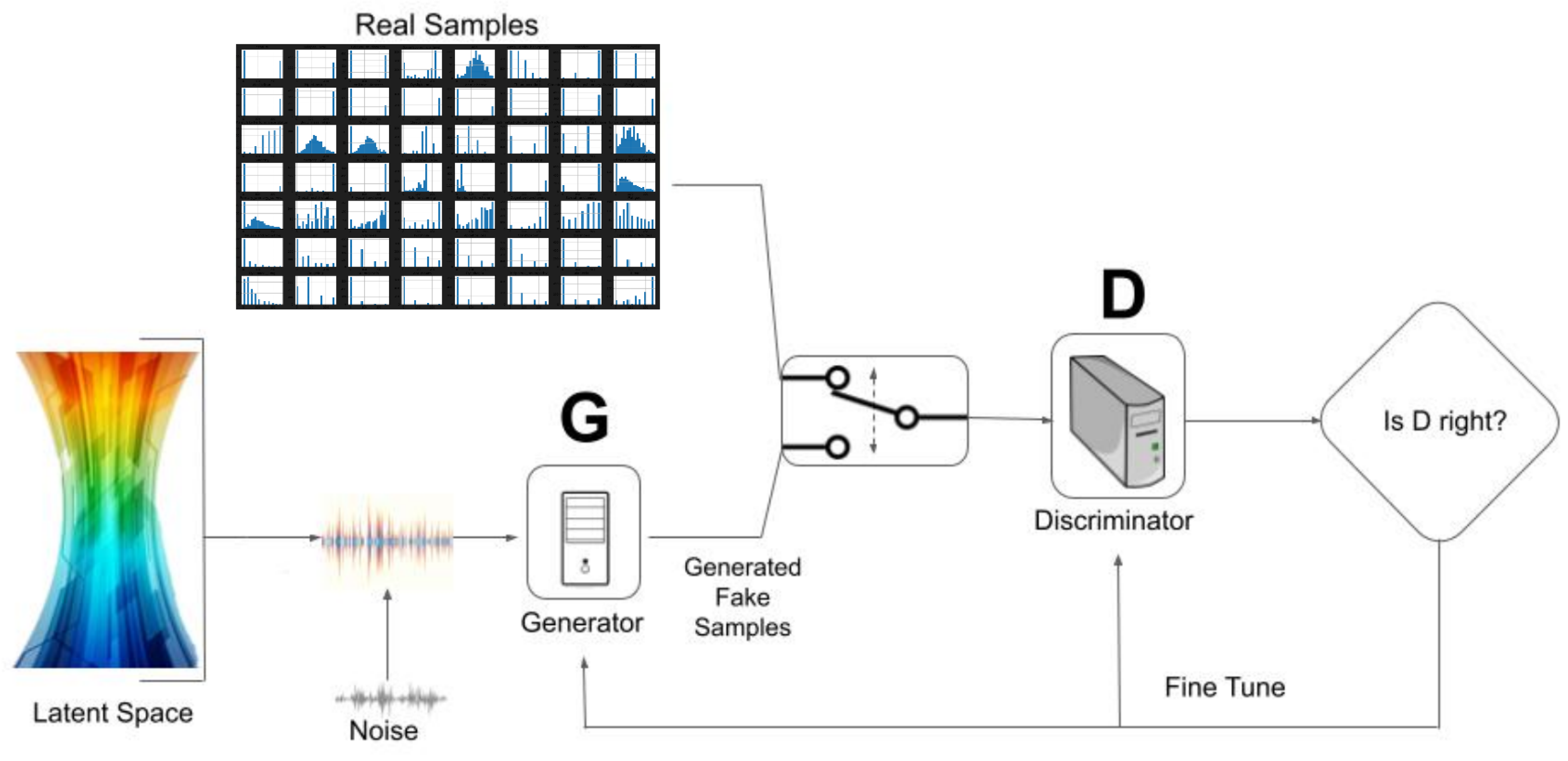
22] are generative models that, in short, work as follows: first, a vector noise is fed into a Generator model (usually an artificial neural network, ANN) to produce synthetic data. Next, generated data are mixed along with real data to feed a Discriminator model (again, usually an ANN), which discriminates which data come from the real dataset and which come from the synthetic data generated from the Generator.
The goal of the Generator is to fool the Discriminator and the goal of the Discriminator is not to be fooled. This confrontation leads to the Generator being increasingly capable of providing synthetic data more similar to real data. The ideal solution in the GAN model is that the percentage of success of the Discriminator for the real data and synthetic data is
, in both cases. The structure of the GAN model for a healthcare database can be seen in
Figure 1.
A brief technical introduction of the GANs model is as follows: given a real sample () and some random noise vector (), the following terms are defined:
is the output of the Discriminator when a real sample is processed.
is the output of the Generator from the noise , that is, the synthetic data.
is the prediction from the Discriminator on the synthetic data.
m is the size of samples.
and are the distribution of real and noise data, respectively.
and are the expected log likelihood from the different outputs of real and generated data.
and are the weights of the Discriminator and Generator model, respectively.
The expression to be considered for the complete network, Discriminator and Generator, is the following, and represents a value,
V,
This value function is submitted to a min–max strategy with the goal to maximize the Discriminator loss and minimize the Generator loss,
The value for the value function V is calculated as the sum of expected log likelihood for real or synthetic samples, and maximizing the resulting values leads to the optimization of the Discriminator parameters so that it learns to correctly identify both real and fake data. A database of real samples (training data) are needed so as to distinguish between real and synthetic data.
The loss function for the discriminator is the following one:
and that for the generator is,
Hence, the implementation of a GAN requires an adequate setup for each employed artificial neuronal network and their training.
2.5. Post-Processing of the Output GAN
The output obtained from the GAN, that is the synthetic data, are quantitative features where values are not necessarily in the range . Hence, a post-processing is carried out as follows:
Firstly, it is taken into account that (i) missing values are represented by , and (ii) a pre-processing step was carried out with the real dataset. Therefore, it is also necessary to consider these treatments for the synthetic dataset. For this, a threshold is considered in order to separate the output GAN in two categories: missing values and given values. The threshold is set to in the range (60 in the range ).
On the other hand, when features are either nominal or ordinal, the first value for them in real data is (90 in the range ); hence, if the output GAN is into , the value is assigned. Similarly, we proceed if the output GAN is higher than 1 in the nominal and ordinal features.
This transformation is also applied to quantitative features since, in this way, in the future, they can be converted into scaled images to , as for the initial data.
Let us name this post-processing as
first transformation. The mathematical expression is as follows:
A second transformation is carried out only for nominal and ordinal features. Thus, given a synthetic value for a feature, it is transformed into the closest real value for this feature.
In order to quantify the impact of these transformations, the loss of the generator is used to quantify the loss between the real data and both the output from the GAN and the transformed output. Examples of quantifying these transformations can be seen in the next section.
3. Experimentation
In this section, the previously exposed methodology is carried out. In addition, the validation of the results obtained is analyzed.
3.1. Missing Values
As mentioned, the percentage of missing values in the data set is 10.88%. It is necessary to reduce this percentage. Thus, a study of the missing values is carried out, and by taking into account medical, statistical (cumulative histograms of the number of missing values) and machine learning criteria, the decision was to choose a maximum number of 26 missing values for each patient and 250 missing values for each feature as selection criterion.
Note that since the number of features is 64, if the threshold (26) is exceeded, it means that the patient has more than missing values, that is, a little less than half of the values are not gathered by the medical team. After applying this filter, there are 58 patients (instances) with more than 26 missing values that are removed from the database. Therefore, the number of patients to be considered in our study is 828.
With respect to the features, since the number of patients is now 828, if the threshold (250) is exceeded, it means that the feature has more than
of missing values. After applying this filter, there exist
features with more than 250 missing values, which are eliminated. Hence, the number of features to be considered is 58. The features eliminated can be seen in
Table 1, where the number of missing values and its percentage is also provided. A detailed description of the number of missing values by each of the 58 considered features can be observed at the end of the manuscript. It is shown that there are only 14 of 58 features with less than 10 missing values.
In our previous study [
2], only statistical criteria (cumulative histograms) were considered, hence only 804 patients, but 64 features composed the original database. This time, according to medical reasons, more patients were taken into consideration (from 804 to 828 patients), because they constitute a more general representation of the cohort. On the other side, some of the eight features left are important from a medical point of view; however, if they were taken into consideration, they greatly degrade the performance of the GAN model.
It can be observed in
Table 2 how the original dataset has been modified. Now, the number of missing values is 2244; that is, in the dataset obtained, there are 3928 less missing values than in the original dataset.
Hence, losing a few patients and a few features, we managed to eliminate more than of the missing data. This means that despite carrying out a huge deletion of missing values, the number of them in the dataset is still relevant for validation purposes.
3.2. Pre-Processing Data
The pre-processing described in
Section 2.3 is carried out on the data set for which the missing data problem has been previously treated. Now, the
value will denote a missing value, and
and 1 are the minimum and the maximum values for all the features, respectively.
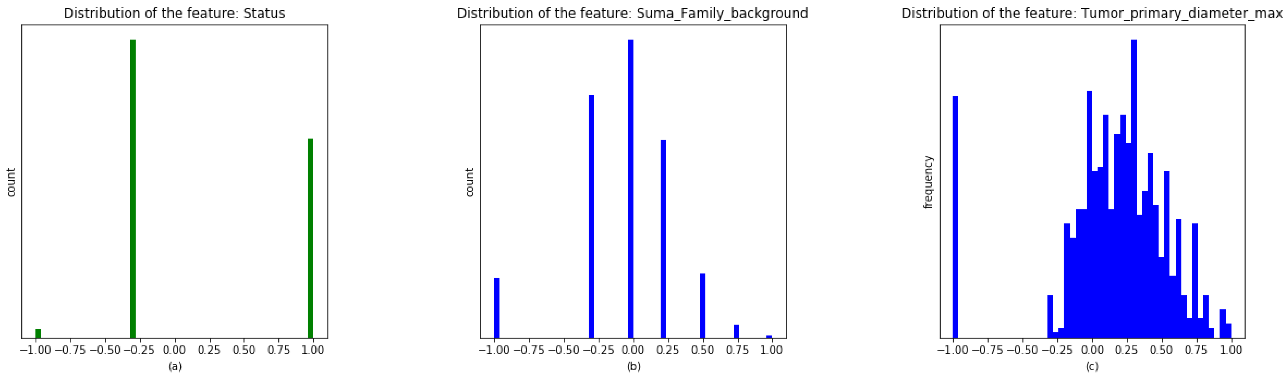
It is illustrated in
Figure 2 how missing values are separated off the real ones for three kinds of features: Boolean (
Figure 2a), ordinal (
Figure 2b) and quantitative (
Figure 2c). The
x-axis shows the values in the new range. The
y-axis represents the count of data if the variable is Boolean, categorical or ordinal and the frequencies if the variable is continuous.
3.3. GAN Setup
In our experimentation, the GAN used has been set up as follows: the size of the inputs in the training of the proposed GAN has been settled to BUFFER_SIZE = 828 (the size of the dataset), BATCH_SIZE = 276 (one-third of the patients (m)) and a noise vector (z) of size 32 by following a uniform distribution in (). The number of EPOCHs is 250 and the experimentation is carried out 60 times.
The architecture for the Generator is composed by eight dense layers of size 1024, 512, 256, 128, 128, 64, 64 and 58, respectively, where the input is the noise vector of size 32 and the output is a vector of size 58, which is the same as the number of features. The architecture for the Discriminator is composed by five dense layers of size 512, 256, 128, 32 and 1, respectively, all of them with batch normalization and leaky (alpha = ) layers. Hence, the number of trainable parameters in Generator and Discriminator ( and ) are 755,514 and 200,449, respectively.
The optimizer used for both, Generator and Discriminator, is the Adam optimizer with the same learning rate equal to . The loss function for the discriminator (D) is based on the cross-entropy loss, because the discriminator performs a binary classification problem. The loss for the generator (G) is based on the mean squared error of the percentiles between real and synthetic data. The number of percentiles used is NQ = 91, which is evenly distributed from 0 to 100. This loss function is selected because by choosing the appropriate number of percentiles, we are able to empirically prove that the goodness-of-fit performance of the real and synthetic distributions can be improved. Furthermore, in order to analyze the stability of the training regime, the Fréchet Inception Distance between real and synthetic data is obtained in each iteration. A threshold value equal to is also set as an early stop of the code.
3.4. Model Selection
In order to run the proposed GAN, a seed is necessary to be provided for the noise vector
. In the ideal case, the Discriminator should provide the same probabilities for the real and synthetic data, that is
[
22]. Hence, we have defined the next function, expressed in percentage, to quantify the quality of the trained GAN structure and select the best one for experimentation:
where
and
are the probabilities given for the Discriminator to real
x and synthetic G(
z) data, respectively. This function is bounded in the range 0 to 100. The value 0 indicates the worst possible performance, and this is followed by a naive discriminator (if it always labels as real, then
and
; and if it always labels as synthetic, then
and
). On the other hand, the value 100 indicates the ideal performance when
. Therefore, if
is close to 100, the performance of the GAN is excellent.
In the experimentation phase, many randomly chosen seeds were implemented and among all of them, the one that received a higher value in the
function was selected. The obtained highest value,
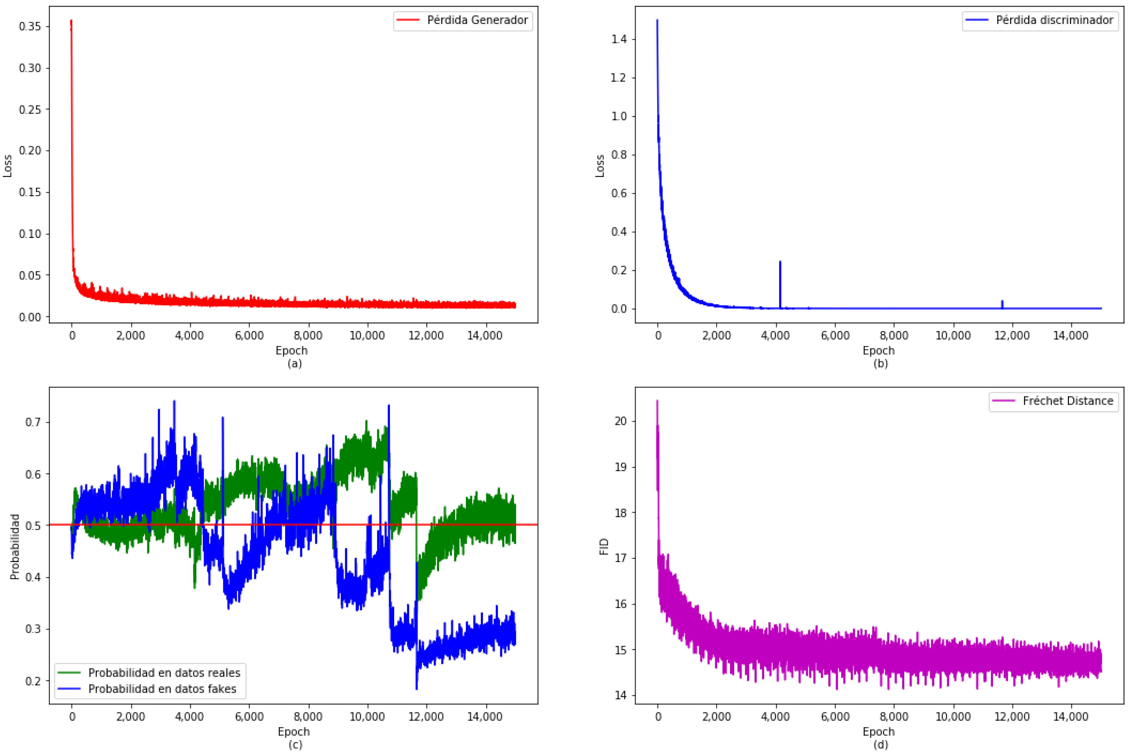
, indicates a very good performance of the chosen model. The result for the training of the proposed GAN on the real dataset is shown in
Figure 3. Both Generator and Discriminator losses are shown in the upper part (
Figure 3a,b), respectively. Both losses are stable when training is finished. The Fréchet Inception Distance, a popular metric for quantifying the distance between two distributions of images [
23], is shown in
Figure 3d, which is also stabilized. The probabilities given by the Discriminator to both, real (in green) and synthetic data (in blue), are shown in
Figure 3c. Let us indicate that these probabilities have not completely stabilized, but this is not totally possible because of the random generation of the batch of real data in the algorithm of the GAN.
3.5. Generation of the Synthetic Dataset
Next, a synthetic dataset with instances (synthetic patients), that is, 20 times the size of the real dataset, is generated. For this synthetic dataset, the accuracy provided by the Discriminator is for the real data, which is very close to the ideal (). In the case of the synthetic data, the accuracy provided by the Discriminator is . This synthetic dataset will be used for testing and validation.
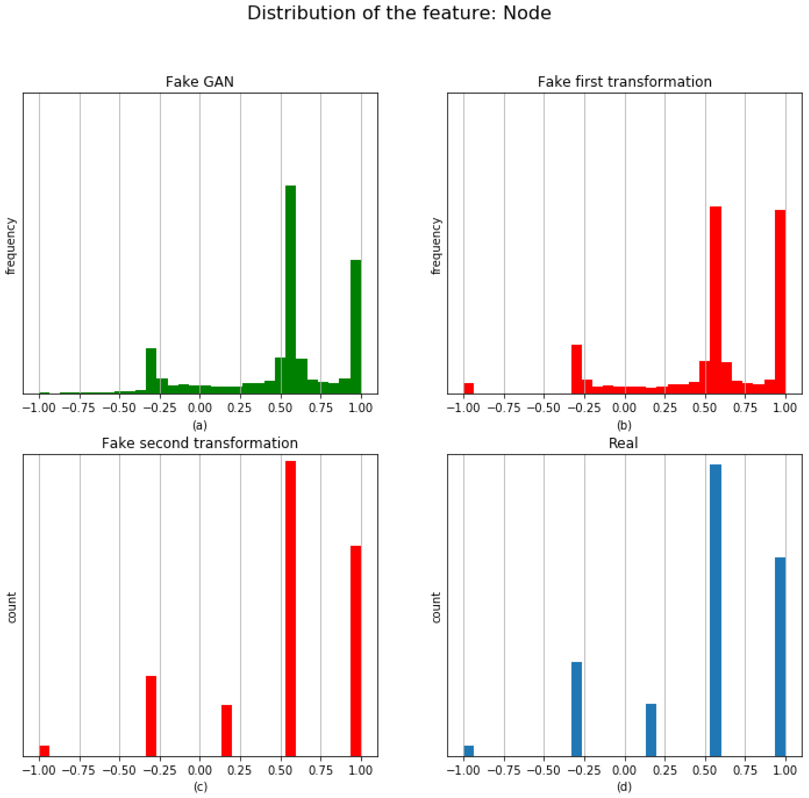
Before carrying out the proposed two post-processing transformations, let us see an example of the distribution generated by the GAN for the feature
Node.
Figure 4 shows the histogram (with 31 bins) of the generated synthetic instances/patients (upper left) and real data (lower right). It can be seen that distributions are not completely similar because the Generator is a model providing quantitative features.
Now, the post-processing presented in
Section 2.5 is carried out. The post-processing is applied to the synthetic data; hence, a new dataset, called the
synthetic-patients dataset, is generated. Before analyzing the performance of the
synthetic-patients dataset, let us see, again for illustrative purposes, the example of the transformations on the feature
Node (see
Figure 4).
In this figure, the histogram from the raw synthetic instances is depicted on the upper left corner. On the upper right corner, the first transformation is applied, and a new histogram is obtained. Next, in the lower part left, the bar charts for the synthetic data after the second transformation can be observed. Finally, bar charts for the real data are depicted in the lower right part.
The value of the loss obtained for the feature Node changes when a transformation is applied. In this case, these values are (loss between real and synthetic data without transformation), (loss between real and synthetic data after the first transformation), and (loss between real and synthetic data after of the two transformations). The loss decreases after the first transformation, but it increases after the second transformation. The final result is worse than the one obtained initially, from a machine learning perspective (loss function), but the real distribution has a similar shape to the real data. In our experimentation, this result has always occurred: that is, the final loss value is always slightly higher than the initial loss value. However, validation using statistical tests is performing very well.
3.6. Validating the Synthetic-Patients Dataset
In order to validate whether the distribution of the
synthetic-patients dataset can be considered similar to the real patients, goodness-of-fit tests on all the features are carried out. Thus, Pearson’s chi-squared test (
) is used if the feature is categorical, and the Kolmogorov–Smirnov test is used otherwise. The null hypothesis to check for each features is:
and the significance level is
. Let us clarify both tests: the chi-squared test checks whether the categorical feature has the same frequencies for the synthetic patients and real patients, and the Kolmogorov–Smirnov compares the underlying continuous distributions for the synthetic patients and real patients from two independent samples.
Furthermore, in Pearson’s chi-squared test, if any bin has an frequency of real patients less than 5, then these bins are combined (added) with its adjacent bins to have significance in the frequency.
The results of these tests are provided in
Table 3.
This table shows the p-value and the decision with respect to ; that is, we can reject hypothesis if the p-value is lower than , and we cannot reject it otherwise. Thus, for p-value , there does not exist sufficient evidence to say that the synthetic distribution of patients is different from the real distribution of patients.
According to the results, there are only 10 tests out of 58 in which the decision is to reject , that is, the synthetic-patient dataset comes from the real patients dataset at a level of significance in 48 of the 58 features (). Let us note that the p-value obtained in the test for the feature Intention is greater than the level of significance at ().
For the features with a p-value less than , it is worth noting that these p-values are very close to 0; that is, the test for these features concludes that the synthetic patients dataset does not come from the real patients distribution. We think that this is the motivation because the Discriminator in the GAN provides a probability for the synthetic data of only , which is lower than . That is, the synthetic data are very similar to the real data but there are some features in which there is a significant difference between synthetic and real data.
Figure 5 shows a graphical comparative of the
features with a
p-value less than
. It is worth noting that in some features, such as for example ’Surgery Type’, which is a non-ordinal feature, from a visual viewpoint, the synthetic and real data are very similar.
In other, as example ‘Administered_Dose’, the visual difference between synthetic and real data is evident.
4. Discussion and Conclusions
High-quality synthetic health data generation is a valuable resource for improving healthcare records. Generative adversarial networks can translate information from lung cancer patients in the form of images so it is possible to capture relationships across the various features in real patients.
The existence of missing values in a database is a great challenge in machine learning. The usual practice is to fill in these missing values following some data imputation procedure. However, data obtained after a medical check-up usually present many missing values. In order to replicate original records, most of these missing values must be also considered as valid data. In our approach, work is developed on a database of real patients with lung cancer where the number of missing values is large.
High-quality synthetic data are obtained using GANs in the opinion of the medical team. However, beyond this empirical evidence, some kind of objective validation tools must be provided. The presented study proposes new tools for model optimization and results validation. The GAN model is selected based on a quality index measuring the performance of the Discriminator. In the ideal case, the Discriminator’s accuracy should be for real and synthetic data. Hence, model optimization is working not only on the loss function but also on the reported accuracy results.
The main contribution of this paper refers to the second tool, which is associated to the statistical validation of the generated synthetic data. Transforming data into numerical features and using Pearson’s chi-squared test for categorical data and the Kolmogorov–Smirnov test otherwise, a test hypothesis can be used with the null hypothesis checking whether the synthetic patients dataset distribution comes from the real patients distribution. Using this statistical test for each one of the considered features, it can be affirmed that the null hypothesis cannot be rejected for most of them, that is 48 out of 58 features (
), as it is shown in
Table 3. The introduced work leads to a very useful tool for validation, as it is statistically ensuring unlimited similar-to-the-original data without compromising the privacy of the original elements.
The study carried out in this paper is a novel approach for the automatic generation and validation of synthetic data in the healthcare domain. A number of limitations is still present. In particular, not all the variables are validated according to the statistical test, even though the overall model is optimized according to the loss function. How model performance varies depending on the percentage of statistically validated features and the loss function value variation is an interesting issue to be analyzed. A similar comparison could be also established with the oncologists’ expert opinion.
The Kolmogorov–Smirnov test is used for continuous non-parametric one-dimension data distribution. It is one of the most used, and arguably most powerful, two-sample tests. However, as a major drawback, it is only applicable in one dimension, whereas many problems in data science cannot be compressed to one dimension without loss of information. A promising research line to be explored is the high-dimensional Kolmogorov–Smirnov distance, as introduced in [
24,
25]. Moreover, it can be combined with the approach in [
26], where a new GAN activation function based on the Smirnov transform is used to faithfully replicate both continuous and discrete random variables.


