Recent Advances in Pulse-Coupled Neural Networks with Applications in Image Processing

Abstract

This paper surveys recent advances in pulse-coupled neural networks (PCNNs) and their applications in image processing. The PCNN is a neurology-inspired neural network model that aims to imitate the information analysis process of the biological cortex. In recent years, many PCNN-derived models have been developed. Research aims with respect to these models can be divided into three categories: (1) to reduce the number of manual parameters, (2) to achieve better real cortex imitation performance, and (3) to combine them with other methodologies. We provide a comprehensive and schematic review of these novel PCNN-derived models. Moreover, the PCNN has been widely used in the image processing field due to its outstanding information extraction ability. We review the recent applications of PCNN-derived models in image processing, providing a general framework for the state of the art and a better understanding of PCNNs with applications in image processing. In conclusion, PCNN models are developing rapidly, and it is projected that more applications of these novel emerging models will be seen in future.

1. Introduction

The pulse-coupled neural network (PCNN) was inspired by animals’ neuronal cortexes. The images received by animals’ eyes stimulate the neurons in their visual cortex, creating spikes and further transmission of spikes between cortical cell assemblies [1,2]. This transmission phenomenon between cell assemblies can recognize and extract the information contained in the stimuli (i.e., the images observed by animals’ eyes) [3]. Evolution has made this working style of biological cortex extremely good at processing the dynamic information inside images. Based on these neurological features, Eckhorn et al. proposed an artificial cortical model [4] that transfers the dynamic information processing property from the biological cortex to the computer. In the interests of image processing, Johnson et al. proposed a PCNN model in 1994 that was based on Eckhorn’s initial cortex model. They concluded that with the limit of weak to moderate liking strength, the periodic time series as signatures of images are invariant to translation, rotation, scale, intensity, and distortion changes in these images [5]. In the following year, Ranganath et al. demonstrated that PCNN exhibits outstanding performance for image smoothing, image segmentation and feature extraction [6]. Since then, the PCNN has found extensive use in image processing areas such as pattern recognition [3], feature extraction [5], image segmentation [6], image shadow removal [7], image encryption [8], and object recognition [9,10].

In 1996, Kinser proposed the simple pulse network (SPN) [11]. This network is more efficient than the original PCNN, having less computational complexity, while exhibiting similar performance to the PCNN. Since then, several modifications and variations of PCNN have been introduced, which have dramatically influenced the image processing field [12]. The intersecting cortical model (ICM) is a representative simplification of the PCNN model, and was designed for image feature enhancement tasks [13]. In 2009, Zhan et al. [14] proposed a spiking cortical model (SCM), which employs simplified equations like the ICM but inherits the linking field from the PCNN. In recent years, the heterogeneous PCNN [15,16,17] and the non-integer step model [18,19] have been proposed. These novel models are undoubtedly becoming popular new research interests in the image processing field. Furthermore, the continuous-coupled neural network (CCNN) was proposed by Liu et al. in 2022 [20,21]. They considered the stochastic characteristics of the PCNN’s pulse generation process, making the response of CCNN to DC and AC stimuli more similar to natural biological cortex neurons.

The PCNN has been one of the most popular models in the image processing field, which can be attributed to its outstanding information analysis ability, rapid processing speed, and lack of pre-training requirements. Two reviews have thoroughly presented the detailed characteristics of PCNN and early PCNN-derived models [22,23]. Hence, the present review will introduce the PCNN, novel PCNN-derived models, and their applications in the image processing field in recent years.

The remainder of this review is organized as follows. In Section 2, the fundamentals of PCNN and its derived models are introduced. In Section 3, the applications of PCNN in imaging processing are presented. Finally, the conclusions of this study are presented in Section 4.

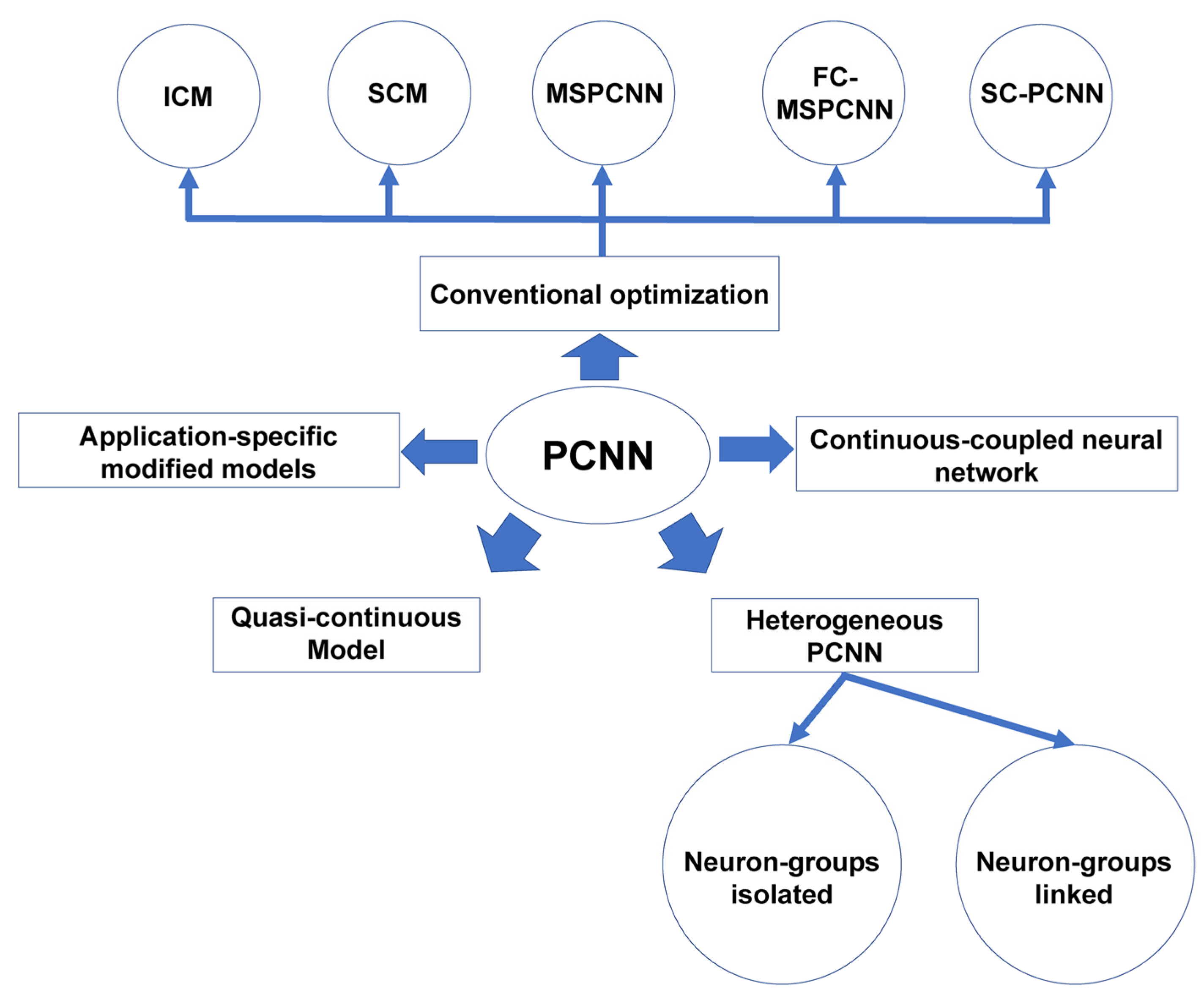
2. Fundamentals of PCNN

The development of PCNN-derived models is shown in Figure 1. Since the initial introduction of PCNN, there have been two significant modification paths of PCNN-derived models: equation simplifications and application-specific optimizations. The first path includes the well-known ICM, SCM, and their further developed models. The second path includes those models generated in practical applications, which are usually only valid for the corresponding applications. In recent years, new PCNN model research has centered on optimizing PCNN models into neural networks that more closely resemble natural biological neural systems. These optimization attempts have led to three novel PCNN-derived models: (1) quasi-continuous models, (2) heterogenous PCNN, and (3) continuous-coupled neural network. The details of the aforementioned PCNN-derived models are illustrated in this section.

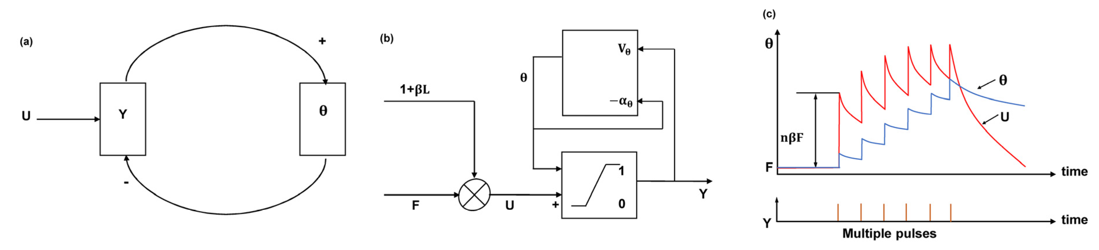
2.1. Original Pulse-Coupled Neural Network

The pulse-coupled neural network is a bio-inspired neuron network based on Eckhorn’s cortical model. It was derived from research on interactions between cell assemblies in a cat’s primary visual cortex [5]. Differing from common neuron networks, the PCNN does not require the pre-training process to form the relationship between input and output data. Instead, the PCNN works in a way similar to real biological neurons, using the change in action potentials when neurons receive stimuli to realize scene analysis. There are three major domains in the PCNN, which are the accepted, modulation, and pulse generator domains. The accepted domain is further divided into two parts: link input and feedback input. The mathematical expressions of PCNN are as follows:

$${\mathit{F}}_{ij}\left[n\right]=e^{-{\alpha }_{\mathrm{F}}}{\mathit{F}}_{ij}\left[n-1\right]+V_{\mathrm{F}}{{\displaystyle \sum }}_{kl}{\mathit{M}}_{ijkl}{\mathit{Y}}_{kl}\left[n-1\right]+{\mathit{S}}_{ij},$$

(1)

$${\mathit{L}}_{ij}\left[n\right]=e^{-{\alpha }_{\mathrm{L}}}{\mathit{L}}_{ij}\left[n-1\right]+V_{\mathrm{L}}{\displaystyle \sum }_{kl}{\mathit{W}}_{ijkl}{\mathit{Y}}_{kl}\left[n-1\right],$$

(2)

$${\mathit{U}}_{ij}\left[n\right]={\mathit{F}}_{ij}\left[n\right]\left\{1+\beta {\mathit{L}}_{ij}\left[n\right]\right\},$$

(3)

$${\mathit{\theta }}_{ij}\left[n\right]=e^{-{\alpha }_{\theta }}{\mathit{\theta }}_{ij}\left[n-1\right]+V_{\theta }{\mathit{Y}}_{ij}\left[n-1\right],$$

(4)

$${\mathit{Y}}_{ij}\left[n\right]=\left\{\begin{array}{c}1, {\mathit{U}}_{ij}\left[n\right]>{\mathit{\theta }}_{ij}\left[n\right]\hfill \\ 0, \mathrm{otherwise}\hfill \end{array}\right.,$$

(5)

where the internal activity of a neuron located at the position $\left(i,j\right)$, ${\mathit{U}}_{ij}$, is determined by the link input ${\mathit{L}}_{ij}$ and feedback input ${\mathit{F}}_{ij}$. The link input and feedback input are coupled by a factor named linking strength $\beta$. $n$ is the iteration count. ${\alpha }_{\mathrm{L}}$ and ${\alpha }_{\mathrm{F}}$ represent the decay time constants of link input and feedback input, respectively. $V_{\mathrm{F}}$ and $V_{\mathrm{L}}$ represent the amplification coefficients of FI and LI, respectively. For a central neuron in the position $\left(i,j\right)$, it is connected with neighboring neurons located at $\left(k,l\right)$ through constant synaptic weight matrixes $\mathit{W}$ and $\mathit{M}$. ${\mathit{S}}_{ij}$ is the input stimulus. ${\mathit{\theta }}_{ij}$ is the dynamic threshold of a neuron in the location $\left(i,j\right)$. ${\alpha }_{\theta }$ is the decay time constant of the dynamic threshold, and $V_{\theta }$ denotes the amplification coefficients of the dynamic threshold. ${\mathit{Y}}_{ij}$ is the timing pulse sequence that determines whether a neuron located at $\left(i,j\right)$ should be fired (${\mathit{U}}_{ij}\left[n\right]>{\mathit{\theta }}_{ij}\left[n\right]$, ${\mathit{Y}}_{ij}\left[n\right]=1$) or not (${\mathit{U}}_{ij}\left[n\right]\le {\theta }_{ij}\left[n\right]$, ${\mathit{Y}}_{ij}\left[n\right]=0$).

As shown in Figure 2a,b [24,25], the internal activity ${\mathit{U}}_{ij}$, timing pulse sequence $\mathit{Y}$, and dynamic threshold ${\mathit{\theta }}_{ij}$ are closely connected. The activity of any one of them will further influence others. Specifically, ${\mathit{U}}_{ij}$ directly influences the $\mathit{Y}$, and $\mathit{Y}$ can further decide ${\mathit{\theta }}_{ij}$. Meanwhile, ${\mathit{\theta }}_{ij}$ in turn affects $\mathit{Y}$ because $\mathit{Y}$ is defined by ${\mathit{U}}_{ij}$ and ${\mathit{\theta }}_{ij}$ together. The ignition condition of a neuron is presented in Figure 2c [24,25]. The internal activity threshold ${\mathit{U}}_{ij}$ and the dynamic threshold ${\mathit{\theta }}_{ij}$ are simultaneously augmented by periodic external input ${\mathit{S}}_{ij}$. After the stimulation of multiple pulses, the growth rate of ${\mathit{U}}_{ij}$ tends to slow down while that of ${\mathit{\theta }}_{ij}$ remains. This phenomenon makes sure that ${\mathit{\theta }}_{ij}$ will eventually exceed ${\mathit{U}}_{ij}$; hence, the reset of a neuron occurs. The number of times when ${\mathit{U}}_{ij}$ is greater than ${\mathit{\theta }}_{ij}$ is defined as the ignition time. The final output of the PCNN is a matrix that has the same dimensions as the original input signal, and each element in this matrix is the ignition time of the input signal’s corresponding position. This output matrix is called as the ignition map.

2.2. Intersecting Cortical Model

The ICM is a representative simplified version of full PCNN. This model includes the feeding input, dynamic threshold, and pulse generator. Its mathematical expressions are as follows:

$${\mathit{F}}_{ij}\left(n+1\right)=\mathrm{𝒻}{\mathit{F}}_{ij}\left(n\right)+{\mathit{S}}_{ij}+{{\displaystyle \sum }}_{kl}{\mathit{W}}_{ijkl}{\mathit{Y}}_{kl}\left(n\right),$$

(6)

$${\Theta }_{ij}\left(n+1\right)=\mathcal{ℊ}{\Theta }_{ij}\left(n\right)+\mathcal{𝒽}{\mathit{Y}}_{ij}\left(n+1\right),$$

(7)

$${\mathit{Y}}_{ij}\left(n+1\right)=\left\{\begin{array}{c}1, if {\mathit{F}}_{ij}\left(n\right)>{\Theta }_{ij}\left(n\right)\hfill \\ 0, otherwise\hfill \end{array}\right.,$$

(8)

where parameters $\mathrm{𝒻}$ and $\mathcal{ℊ}$ are two constant parameters that control the property of the threshold ${\Theta }_{ij}$. $\mathrm{𝒻}$ is a parameter that decides the characteristic of feeding input ${\mathit{F}}_{ij}.$ It is larger than $\mathcal{ℊ}$ to make sure that the threshold finally falls below the feeding input ${\mathit{F}}_{ij}$, making the neuron capable of being ignited. $\mathcal{𝒽}$ is a larger value than $\mathrm{𝒻}$ and $\mathcal{ℊ}$ because the threshold needs to increase substantially to ensure the neuron can be reset after its ignition. The weight matrix $\mathit{W}$ denotes the connections between neurons. Other parameters are the same as those in the original PCNN.

2.3. Spiking Cortical Model

The SCM, introduced by Zhan et al. [14], is a local-connected neural network model derived from the PCNN model. It has fewer parameters, lower computational complexity, and higher accuracy rates compared with PCNN and other PCNN-derived methods such as ICM. Working like a group of real biologic neurons, the membrane potential of a neuron in SCM is calculated by the combination of the direct stimulus, and the synaptic modulation which comes from its neighboring neurons. If the membrane potential of a neuron exceeds its dynamic threshold, this neuron is activated, and it will generate a spike that would further affect its neighboring neurons in the next iteration. The formulae of the SCM are given as follows:

$${\mathit{U}}_{ij}\left(n\right)=f{\mathit{U}}_{ij}\left(n-1\right)+{\mathit{S}}_{ij}(1+{\displaystyle \sum }_{kl}{\mathit{W}}_{ijkl}{\mathit{Y}}_{kl}\left(n-1\right)),$$

(9)

$${\mathit{\theta }}_{ij}\left(n\right)=g{\mathit{\theta }}_{ij}\left(n-1\right)+h{\mathit{Y}}_{ij}\left(n\right),$$

(10)

$${\mathit{Y}}_{ij}\left(n\right)=\left\{\begin{array}{c}1, if {\mathit{U}}_{ij}\left(n\right)>{\mathit{\theta }}_{ij}\left(n-1\right)\hfill \\ 0, otherwise\hfill \end{array}\right.$$

(11)

where $n$ represents the iteration count, ${\mathit{U}}_{ij}\left(n\right)$ denotes a neuron’s membrane potential that is located at $\left(i,j\right)$ at iteration $n$. $f$ is the attenuation constant of the membrane potential, ${\mathit{S}}_{ij}$ represents the external stimulus, ${\mathit{W}}_{ijkl}$ denotes the synaptic weight matrix that affects the connection between a neuron at location $\left(i,j\right)$ and its neighboring neurons at location $\left(k,l\right)$, $\mathit{Y}$ stands for the output action potential (i.e., the output spike) of a neuron, the convolution of ${\mathit{W}}_{ijkl}$ and ${\mathit{Y}}_{kl}\left(n-1\right)$ represents the modulation on the central neuron located at $\left(i,j\right)$ by its neighboring neurons at location $\left(k,l\right)$, ${\mathit{\theta }}_{ij}$ is the dynamic threshold of a neuron at location $\left(i,j\right)$, $g$ and $h$ are the attenuation constant of the threshold and the absolute refractory period, respectively, which prevents neurons that just been activated from being reactivated immediately.

2.4. Modified SPCNN

The modified SPCNN (MSPCNN) model [26] was proposed based on Chen et al.’s simplified pulse-coupled neural network (SPCNN) model [27]. The SPCNN is a simplified version of the original PCNN, with fewer equations and parameters. However, its parameters are not fully automatic, which makes the application of SCPNN limited. The MSPCNN focused on solving this drawback, simplifying the five parameters of SPCNN into three. Moreover, these three parameters are all correlated with the Otsu thresholding [28]. Consequently, all parameters of MSPCNN can be adaptively selected by finding the Otsu thresholding. The mathematical expression of SPCNN is as follows:

$${\mathit{F}}_{ij}\left(n\right)={\mathit{S}}_{ij},$$

(12)

$${\mathit{L}}_{ij}\left[n\right]=V_{\mathrm{L}}{{\displaystyle \sum }}_{kl}{\mathit{W}}_{ijkl}{\mathit{Y}}_{kl}\left[n-1\right],$$

(13)

$${\mathit{U}}_{ij}\left[n\right]=e^{-{\alpha }_f}{\mathit{U}}_{ij}\left[n-1\right]+{\mathit{S}}_{ij}(1+\beta V_{\mathrm{L}}{{\displaystyle \sum }}_{kl}{\mathit{W}}_{ijkl}{\mathit{Y}}_{kl}\left[n-1\right]),$$

(14)

$${\mathit{\theta }}_{ij}\left[n\right]=e^{-{\alpha }_{\theta }}{\mathit{\theta }}_{ij}\left[n-1\right]+V_{\theta }{\mathit{Y}}_{ij}\left[n-1\right],$$

(15)

$${\mathit{Y}}_{ij}\left[n\right]=\left\{\begin{array}{c}1,{ \mathit{U}}_{ij}\left[n\right]>{\mathit{\theta }}_{ij}\left[n\right]\hfill \\ 0, \mathrm{otherwise}\hfill \end{array}\right.,$$

(16)

where all parameters have the same meanings as the original PCNN. The weight ${\mathit{W}}_{ijkl}$ is given as a fixed matrix:

$${\mathit{W}}_{ijkl}=\left[\begin{array}{ccc}0.5& 1& 0.5\\ 1& 0& 1\\ 0.5& 1& 0.5\end{array}\right],$$

(17)

As is apparent, there are five adjustable parameters in the SCPNN: $V_{\mathrm{L}}$, ${\alpha }_f$, $\beta$, ${\alpha }_{\theta }$, and $V_{\theta }$. In the MSPCNN, the mathematical model is the same as that of SPCNN, while $V_{\mathrm{L}}$ is removed, and ${\alpha }_f$ and ${\alpha }_{\theta }$ are combined into one parameter $\alpha$. The remaining three parameters are expressed as follows:

$$\alpha ={\alpha }_f={\alpha }_{\theta }=\log \left(\frac{1}{S^{\prime }}\right),$$

(18)

$$\beta =\frac{1-S^{\prime }}{4S^{\prime }},$$

(19)

$$V_{\theta }=1+{S^{\prime }}^2-{S^{\prime }}^8,$$

(20)

where $S^{\prime }$ denotes the normalized Otsu thresholding.

2.5. Fire-Controlled MSPCNN

The fire-controlled MSPCNN (FC-MSPCNN) is a further model developed based on the MSPCNN, which aims to control the neuronal firing states at each iteration [29]. This FC-MSCPCNN has been proved to work well in general image processing tasks, such as color image quantization and gallbladder image location. It uses parameters with adaptive values rather than fixed parameters of the MSPCNN, and all parameters are automatically set according to the neuronal firing states. These characteristics allow it to overcome the limitations of the MSPCNN in general image processing applications resulting from the randomness and unpredictability of neuronal firing results. The mathematical expression of FC-MSPCNN is given as follows:

$${\mathit{U}}_{ij}\left[n\right]=e^{-\alpha }{\mathit{U}}_{ij}\left[n-1\right]+{\mathit{S}}_{ij}(1+\beta {\displaystyle \sum }_{kl}{\mathit{W}}_{ijkl}{\mathit{Y}}_{kl}\left[n-1\right]),$$

(21)

$${\mathit{\theta }}_{ij}\left[n\right]=e^{-\alpha }{\mathit{\theta }}_{ij}\left[n-1\right]+V_{\theta }{R}_n{\mathit{Y}}_{ij}\left[n-1\right],$$

(22)

$${\mathit{Y}}_{ij}\left[n\right]=\left\{\begin{array}{c}1, {\mathit{U}}_{ij}\left[n\right]>{\mathit{\theta }}_{ij}\left[n\right]\hfill \\ 0, \mathrm{otherwise}\hfill \end{array}\right.,$$

(23)

where $R_n$ is a parameter used to prevent a neuron from firing twice, and other parameters are the same as those in MSPCNN. Additionally, a parameter $P$ is introduced to determine the iteration times of the model. It denotes the iteration times that all the neurons fire once after the first iteration, which is expressed as follows:

$$P=N-1,$$

(24)

where $N$ is the total iteration times of an image processing task. Based on the iteration states and pixel intensity of an image, all other parameters can be expressed as follows:

$$\alpha =-\ln \frac{{\mathit{S}}_{min}}{P},$$

(25)

$$\beta =\frac{1}{4}{e}^{-2\alpha },$$

(26)

$$V_{\theta }=e^{-\alpha }\frac{1-e^{-3\alpha }}{1-e^{-\alpha }},$$

(27)

$$R_n={\left(\frac{e^{N\alpha }}{1-e^{-\alpha }}\right)}^{\sqrt{{\log }_2\left(n\right)}},$$

(28)

where ${\mathit{S}}_{min}$ is the minimum external input, i.e., the minimum pixel intensity of an image.

2.6. Sine–Cosine PCNN

The sine–cosine PCNN (SC-PCNN) was proposed by Yang et al. to suppress random noise [30]. They concluded that the random noise in the PCNN model mainly comes from three sources: the input noise from $\mathit{S}$, system noise from $\mathit{U}$, and a random stat in which $\mathit{\theta }$ is initially randomized. This random noise has a negative influence on the image processing performance of PCNN. To reduce this random noise, they added the sine–cosine term to the PCNN model, using the small oscillations caused by this term to offset the random noise. The mathematical expression of SC-PCNN is as follows:

$${\mathit{U}}_{ij}\left[n\right]=\sin \left(\frac{\pi }{2}\left(1+n\tilde{\alpha }\right)\right){\mathit{U}}_{ij}\left[n-1\right]+{\mathit{S}}_{ij}(1+\beta V_L{\displaystyle \sum }_{kl}{\mathit{W}}_{ijkl}{\mathit{Y}}_{kl}\left[n-1\right]),$$

(29)

$${\mathit{\theta }}_{ij}\left[n\right]=\cos \left(\frac{\pi }{2}\left(1+n\tilde{\alpha }\right)\right){\mathit{\theta }}_{ij}\left[n-1\right]+V_{\theta }{\mathit{Y}}_{ij}\left[n-1\right],$$

(30)

$${\mathit{Y}}_{ij}\left[n\right]=\left\{\begin{array}{c}1, {\mathit{U}}_{ij}\left[n\right]>{\mathit{\theta }}_{ij}\left[n\right]\hfill \\ 0, \mathrm{otherwise}\hfill \end{array}\right.,$$

(31)

where $\tilde{\alpha }$ is a decay factor, set as a fixed number 0.01, and other parameters have the same meaning as those of the MSPCNN. $V_L$ is set as a fixed number 1. The weight ${\mathit{W}}_{ijkl}$, $\beta$, and $V_{\theta }$ are given as follows:

$${\mathit{W}}_{ijkl}=\left[\begin{array}{ccc}0.5& 1& 0.5\\ 1& 0& 1\\ 0.5& 1& 0.5\end{array}\right],$$

(32)

$$\beta =\frac{\frac{{\mathit{S}}_{max}}{S^{\prime }}-1}{V_L\sum {\mathit{W}}_{ijkl}},$$

(33)

$$V_{\theta }=\frac{{\mathit{S}}_{max}}{S^{\prime }},$$

(34)

where ${\mathit{S}}_{max}$ is the maximum pixel intensity and $S^{\prime }$ denotes the normalized Otsu thresholding.

2.7. Quasi-Continuous Model

The quasi-continuous model (or non-integer step index PCNN model) was proposed to solve the mathematical coupled firing phenomenon. This model uses non-integer steps to emulate a continuous time system. In the early stage of the PCNN’s development, the network system was constructed discretely due to the significant computational costs [31]. With advances in computer science, the computational ability of modern computers is able to bear the computational burden of the continuous-time PCNN system. Therefore, the quasi-continuous model is proposed, making it possible to adjust the balance between the PCNN’s resolution and computational complexity [32]. The mathematical expression of the quasi-continuous model is as follows:

$${\mathit{W}}_{ijkl}=\left[\begin{array}{ccc}0.5& 1& 0.5\\ 1& 0& 1\\ 0.5& 1& 0.5\end{array}\right],$$

(35)

$$\beta =\frac{\frac{{\mathit{S}}_{max}}{S^{\prime }}-1}{V_L\sum {\mathit{W}}_{ijkl}},$$

(36)

$$V_{\theta }=\frac{{\mathit{S}}_{max}}{S^{\prime }},$$

(37)

$${\mathit{U}}_{ij}\left(t+\mathrm{\Delta }t\right)=e^{-{\alpha }_F\mathrm{\Delta }t}{\mathit{U}}_{ij}\left(t\right)+{\mathit{S}}_{ij}(1+\beta {\displaystyle \sum }_{kl}{\mathit{W}}_{ijkl}{\mathit{Y}}_{kl}\left(t\right)),$$

(38)

$${\mathit{\theta }}_{ij}\left(t+\mathrm{\Delta }t\right)=e^{-{\alpha }_E\mathrm{\Delta }t}{\mathit{\theta }}_{ij}\left(t\right)+V_{\theta }{\mathit{Y}}_{ij}\left(t\right),$$

(39)

$${\mathit{Y}}_{ij}\left(t+\mathrm{\Delta }t\right)=\left\{\begin{array}{c}1, if {\mathit{U}}_{ij}\left(t+\mathrm{\Delta }t\right)>{\mathit{\theta }}_{ij}\left(t\right)\hfill \\ 0, otherwise\hfill \end{array}\right.,$$

(40)

where $\mathrm{\Delta }t$ is a non-integer scale that decides the resolution of this model and other parameters are the same as those in MSPCNN. When $\mathrm{\Delta }t$ is closer to 0, the model becomes more similar to a continuous-time system. In contrast, when $\mathrm{\Delta }t$ is closer to 1, the model becomes more similar to the discrete SPCNN model. The non-integer step model has been demonstrated to be highly effective in applications that need fine resolution and the detection of small details, such as image noise analyses and detection of micro-calcifications.

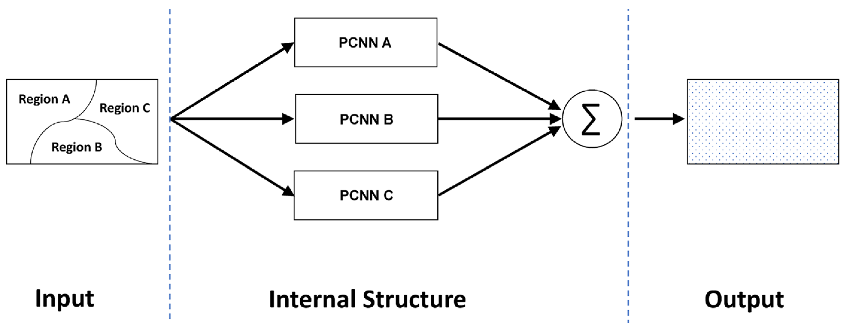
2.8. Heterogeneous PCNN

Biological findings have shown that animals’ nervous systems are heterogeneous in terms of both their structures and the interconnections between neurons [33,34,35]. To make the PCNN model closer to natural nervous systems, the heterogeneous PCNN (HPCNN) has been proposed. The heterogeneous aspect of HPCNN incorporates the following three types:

•  Neurons with different weights, but the same structure.
•  Neurons with different structures, but the same weight.
•  Both structure and weight are different for different neurons.

Apparently, the third type is the closest to the real neuron cortex structure. However, different weights and different neuron characteristics lead directly to a large number of manual parameters. For example, if an image is divided into three parts and processed by three different PCNN models, three times the number of parameters will be needed compared to the homogeneous PCNN. Only in a few image processing applications can the parameters of PCNN be fully automatic, making the parameter selection task of the other applications extremely cumbersome. Even in adaptive parameter applications, such as image segmentation, the computational complexity still curtails the finer classification of an image (i.e., using more different PCNN models to process a single image). Although there are drawbacks to HPCNN that remain unsolved, the image processing performance of HPCNN is impressive, and it is undeniably becoming one of the most popular research interests in the PCNN field. HPCNN models can be categorized into two types: neuron groups-isolated models and neuron groups-linked models.

The first type is represented by the initial HPCNN model proposed by Huang et al. [15]. The neuron structure of their model is shown in Figure 3. This group-isolated HPCNN model divides an image into different parts and processes different parts with different PCNN models. There is no link between different PCNN models, which means that the firing condition of a PCNN model will not influence other PCNN models, and the final output of the HPCNN is the summation of all independent PCNN models. The mathematical expression of each independent PCNN is the same as the original PCNN model. An automatic parameter decision strategy is designed to select parameter values of different PCNN models based on the characteristics of different image parts.

The second type is represented by the heterogeneous SPCNN (HSPCNN) proposed by Yang et al. [36]. The neuron structure of their model is shown in Figure 4 [36]. Similar to the first type, the HSPCNN is constructed by serval different SPCNN models, and each SPCNN model is responsible for the image processing task of an image’s particular part. However, in the neuron groups-linked HSPCNN model, different SPCNN models are connected by the weight $L_{12}$ and $L_{23}$. This connection allows the HSPCNN able to process an image in a way that is more similar to the natural cortex of animals. This is realized through the parameter and formula simplification of the SPCNN model. For each SPCNN model, the formulas are the same as the SPCNN model described in Section 2.4, and all parameters are decided without a manual process. The final output of the HSPCNN is obtained by summing up the results of different SPCNN models.

2.9. Continuous-Coupled Neural Network

The continuous-coupled neural network (CCNN) is the most recent advance in PCNN-related models, proposed by Liu et al. in 2022 [20,21]. The CCNN is an attempt to push brain-like computation even further. Unlike all current deep learning neuron networks, PCNN is one of the most successful third generation models, which use spiking to translate and analyze information, a method that mammals have evolved over hundreds of millions of years. However, a chaos phenomenon called the “butterfly effect” that has long been known in the electrophysiological field [37] cannot be simulated by PCNN or PCNN-derived models. Specifically, neurophysiological evidence shows that neurons exhibit chaotic behavior under a periodic stimulus and periodic behavior under a constant stimulus. In contrast, PCNN cannot exhibit these characteristics.

Consequently, the CCNN is proposed to solve the gap between the response characteristics of PCNN and natural neurons. Specifically, the CCNN uses sigmoid functions to replace PCNN’s pulse generator and considers the stochastic attributes of the pulse generation process. The formulas of CCNN are as follows:

$${\mathit{F}}_{ij}\left[n\right]=e^{-{\alpha }_{\mathrm{F}}}{\mathit{F}}_{ij}\left[n-1\right]+V_{\mathrm{F}}{\displaystyle \sum }_{kl}{\mathit{M}}_{ijkl}{\mathit{Y}}_{kl}\left[n-1\right]+{\mathit{S}}_{ij},$$

(41)

$${\mathit{L}}_{ij}\left[n\right]=e^{-{\alpha }_{\mathrm{L}}}{\mathit{L}}_{ij}\left[n-1\right]+V_{\mathrm{L}}{\displaystyle \sum }_{kl}{\mathit{W}}_{ijkl}{\mathit{Y}}_{kl}\left[n-1\right],$$

(42)

$${\mathit{U}}_{ij}\left[n\right]={\mathit{F}}_{ij}\left[n\right]\left\{1+\beta {\mathit{L}}_{ij}\left[n\right]\right\},$$

(43)

$${\mathit{\theta }}_{ij}\left[n\right]=e^{-{\alpha }_{\theta }}{\mathit{\theta }}_{ij}\left[n-1\right]+V_{\theta }{\mathit{Y}}_{ij}\left[n-1\right],$$

(44)

$${\mathit{Y}}_{ij}\left[n\right]=\frac{1}{1+e^{-\left({\mathit{U}}_{ij}\left[n\right]-{\mathit{\theta }}_{ij}\left[n\right]\right)}},$$

(45)

where all parameters have the same meanings as in the original PCNN model. It is worth noting that the CCNN exhibits outstanding performance on video processing tasks. It encodes changing pixels as non-periodic chaotic signals and static pixels as periodic signals, making it capable of recognizing objects directly. This method of object recognition is different from all other video processing algorithms, in that it employs no feature extraction process.

Aside from the aforementioned PCNN-derived models, some other research has been performed during the past few years, in areas such as three-dimensional PCNN [38], color transfer PCNN [39], and pulse-number-adjustable MSPCNN [40]. These studies have modified the general PCNN-derived models, making them more suitable for specific applications. This application-driven PCNN modification is becoming a new research hot zone in the fields of image processing, video processing, automatic diagnostics, and many other areas. The details of these novel PCNN applications will be presented in the next section.

3. Applications

PCNN applications in the image processing field were illustrated in 2018 by Zhen et al. [23]. Since then, applications of PCNN-derived models have expanded dramatically in just a few years. It is hard to present all the novel applications in a thorough manner; hence, we present some representative applications in three main categories: (1) color image processing, (2) diagnosis and computer vision, and (3) image fusion. The advantages exhibited by the PCNN in these novel applications are analyzed in order to shed light on current trends and possible future research topics in PCNN-related image processing fields.

3.1. Color Image Processing

Jia et al. presented a three-dimensional PCNN (3DPCNN) for oil pollution image segmentation [38]. They combined the 3DPCNN with a hybrid seagull optimization algorithm to analyze the pollution condition of an image. The color information inside the red, green, and blue (RGB) channels is crucial in the segmentation task of oil pollution. It is necessary to use all information in these channels, which necessitates modifying the PCNN to process RGB channels simultaneously. Consequently, each neuron is connected with 26 neighboring neurons in the 3DPCNN model. The inter- and intra-channel spike transmission efficiently extracts information from color images, leading to state-of-art segmentation performance. He et al. proposed a color transfer PCNN for enhancing the underwater visual images captured by robots [39]. This algorithm can process retrieved images in real time and improve their color and contrast. Unlike the 3DPCNN, the color transfer PCNN processes color images in the HSI space (hue, saturation, and intensity), rather than the RGB space. An image is separated into H, S, and I components and fed to three independent PCNNs. This PCNN enhancement process successfully produces more edges and detail.

The PCNN-based color image processing algorithms are currently the closest kind to biological color vision. On the one hand, three types of retinal cells in the human eye are sensitive to different wavelengths of light. The wavelength information they collect is processed through spike transmission in the cortex, generating color images in the brain. This process corresponds to the 3DPCNN model. On the other hand, human vision perceives brightness much more strongly than color intensity. Transforming images to the HIS space is suitable for representing the characteristics of human vision. This process corresponds to color transfer PCNN. Further research on PCNN-based color image processing is helpful for scientists to better understand the working style of the human visual system.

3.2. Diagnosis and Computer Vision

In 2021, Shanker et al. proposed a fast version of SPCNN [41]. They combined it with the Ripplet transform, probabilistic principal component analysis, and twin support vector machine to construct an automated computer-aided diagnosis system. This system exhibited state-of-art brain magnetic resonance image analysis ability. A deep learning model based on the PCNN and transfer learning was proposed in 2021 [42], focusing on breast cancer diagnosis. Moreover, Thyagharajan et al. proposed a PCNN-based near-duplicate detection algorithm [43]. They used the PCNN to extract features from the near-duplicated images, generating feature maps for subsequent image similarity measurement.

These applications use the advantages of PCNN in that it is able to segment images and process low-resolution images without requiring any pre-processing steps. Performing operations on the original image is cumbersome and expensive in many image processing scenarios. Consequently, a method that can automatically select a region of interest or extract a feature map is important. PCNN-derived models are competent for these tasks and can exhibit state-of-the-art performance with no pre-training process. They have become popular methods in the image segmentation field [44,45].

3.3. Image Fusion

As a result of PCNN’s excellent feature extraction ability, its application in the image fusion field has been extensively researched in recent years, for example, in muti-focus image fusion [46,47] and multimodal medical image fusion [48,49,50]. In these fusion applications, the PCNN mainly serves as a fusion decision method. It is combined with other methods such as image decomposition transforms and texture analysis [51,52]. The pixels with important information inside the decomposition images or feature images are selected by PCNN. The final fused image is reconstructed on the basis of these selected pixels.

3.4. Other Recent Advances

In 2021, Chen et al. used the PCNN to achieve real-time auto-focusing control [53]. Lian et al. proposed a pulse-number-adjustable MSPCNN (PNA-MSPCNN) for the image enhancement task in 2021 [40]. This PNA-MSPCNN was able to adaptively select each neuron’s firing times and frequency, achieving impressive low-light image enhancement performance. The directional PCNN is offered for dynamic gesture recognition [54], which can prevent irrelevant neurons from firring in order to realize rapid recognition while maintaining high accuracy. The heterogenous PCNN-based hyperspectral image visualization technique was achieved by Duan et al. in 2019 [17], indicating the potential of HPCNN’s application in areas other than image segmentation and quantization.

In these recent advances, novel PCNN-derived models such as the HPCNN were used to achieve cutting-edge image processing performance. The rapid development of the PCNN family is undoubtedly influencing and propelling advances in image processing fields.

3.5. Summary

Generally, making modifications to PCNN specific to the application requirements and combining PCNN-derived models with conventional algorithms within the application fields are the two main streams of PCNN applications. The most significant advantages of PCNN in the image processing field are: (1) the lack of a pre-training requirement; (2) outstanding feature extraction and image segmentation abilities; and (3) the ability to process images under various resolution conditions. However, the following disadvantages of PCNN remain unsolved: (1) parameter selection strategy; and (2) computational cost. Nowadays, the parameters are decided empirically, either using an empirical formula or on the basis of extensive experiments. A general parameter decision methodology is a crucial research topic for the future. Moreover, the applications of three recently proposed PCNN models—quasi-continuous models, HPCNN, and CCNN—are still in the early stages. It is expected that more applications of these models will be seen in the future.

4. Conclusions

As a bio-neuron-inspired network, the PCNN has been successfully applied in the image processing field. This paper reviews the development of PCNN models and their applications in image processing. The development of PCNN-derived models can be categorized into five groups: (1) conventional optimization models, (2) application-specific modified models, (3) quasi-continuous models, (4) heterogeneous PCNN, and (5) continuous-coupled neural networks. Representative models and recent developments in each category are discussed. Recent developments in the image processing area can be divided into two primary research interests: (1) modify PCNN models specific to the application requirements, and (2) combine PCNN-derived models with conventional algorithms within the application field. The application of novel models, such as the quasi-continuous and continuous-coupled neural network, are in their infant stage. More research related to them is projected to emerge in the future.

References

1. Freeman, W.J.; van Dijk, B.W. Spatial patterns of visual cortical fast EEG during conditioned reflex in a rhesus monkey. Brain Res. 1987, 422, 267–276. [Google Scholar] [CrossRef]
2. Eckhorn, R.; Bauer, R.; Jordan, W.; Brosch, M.; Kruse, W.; Munk, M.; Reitboeck, H.J. Coherent oscillations: A mechanism of feature linking in the visual cortex? Biol. Cybern. 1988, 60, 121–130. [Google Scholar] [CrossRef] [PubMed]
3. Hodgkin, A.L.; Huxley, A.F. A quantitative description of membrane current and its application to conduction and excitation in nerve. J. Physiol. 1952, 117, 500–544. [Google Scholar] [CrossRef] [PubMed]
4. Eckhorn, R.; Reitboeck, H.J.; Arndt, M.; Dicke, P. Feature Linking via Synchronization among Distributed Assemblies: Simulations of Results from Cat Visual Cortex. Neural Comput. 1990, 2, 293–307. [Google Scholar] [CrossRef]
5. Johnson, J.L. Pulse-coupled neural nets: Translation, rotation, scale, distortion, and intensity signal invariance for images. Appl. Opt. 1994, 33, 6239–6253. [Google Scholar] [CrossRef] [PubMed]
6. Ranganath, H.S.; Kuntimad, G.; Johnson, J.L. Pulse coupled neural networks for image processing. In Proceedings of the Proceedings IEEE Southeastcon ‘95. Visualize the Future, Raleigh, NC, USA, 26–29 March 1995; pp. 37–43. [Google Scholar]
7. Gu, X.; Yu, D.; Zhang, L. Image shadow removal using pulse coupled neural network. IEEE Trans. Neural Netw. 2005, 16, 692–698. [Google Scholar] [CrossRef] [PubMed]
8. Liu, M.; Zhao, F.; Jiang, X.; Zhang, H.; Zhou, H. Parallel binary image cryptosystem via spiking neural networks variants. Int. J. Neural Syst. 2021, 32, 2150014. [Google Scholar] [CrossRef] [PubMed]
9. Ranganath, H.S.; Kuntimad, G. Object detection using pulse coupled neural networks. IEEE Trans. Neural Netw. 1999, 10, 615–620. [Google Scholar] [CrossRef]
10. Yu, B.; Zhang, L. Pulse-coupled neural networks for contour and motion matchings. IEEE Trans. Neural Netw. 2004, 15, 1186–1201. [Google Scholar] [CrossRef]
11. Jason, M.K. Simplified pulse-coupled neural network. In Applications and Science of Artificial Neural Networks; SPIE: Bellingham, WA, USA, 1996. [Google Scholar]
12. Johnson, J.L.; Padgett, M.L. PCNN models and applications. IEEE Trans. Neural Netw. 1999, 10, 480–498. [Google Scholar] [CrossRef]
13. Ekblad, U.; Kinser, J.M.; Atmer, J.; Zetterlund, N. The intersecting cortical model in image processing. Nucl. Instrum. Methods Phys. Res. Sect. A Accel. Spectrometers Detect. Assoc. Equip. 2004, 525, 392–396. [Google Scholar] [CrossRef]
14. Zhan, K.; Zhang, H.; Ma, Y. New Spiking Cortical Model for Invariant Texture Retrieval and Image Processing. IEEE Trans. Neural Netw. 2009, 20, 1980–1986. [Google Scholar] [CrossRef]
15. Huang, Y.; Ma, Y.; Li, S.; Zhan, K. Application of heterogeneous pulse coupled neural network in image quantization. J. Electron. Imaging 2016, 25, 61603. [Google Scholar] [CrossRef]
16. Huang, Y.; Ma, Y.; Li, S. A new method for image quantization based on adaptive region related heterogeneous PCNN. In Proceedings of the International Symposium on Neural Networks, Jeju, Korea, 15–18 October 2015; pp. 269–278. [Google Scholar]
17. Duan, P.; Kang, X.; Li, S.; Ghamisi, P. Multichannel Pulse-Coupled Neural Network-Based Hyperspectral Image Visualization. IEEE Trans. Geosci. Remote Sens. 2020, 58, 2444–2456. [Google Scholar] [CrossRef]
18. Yang, Z.; Dong, M.; Guo, Y.; Gao, X.; Wang, K.; Shi, B.; Ma, Y. A new method of micro-calcifications detection in digitized mammograms based on improved simplified PCNN. Neurocomputing 2016, 218, 79–90. [Google Scholar] [CrossRef]
19. Yang, Z.; Guo, Y.; Gong, X.; Ma, Y. A Non-integer Step Index PCNN Model and Its Applications. In Medical Image Understanding and Analysis; Springer: Cham, Switzerland, 2017; pp. 780–791. [Google Scholar]
20. Liu, J.; Lian, J.; Sprott, J.C.; Liu, Q.; Ma, Y. The Butterfly Effect in Primary Visual Cortex. IEEE Trans. Comput. 2022, 1. [Google Scholar] [CrossRef]
21. Liu, J.; Lian, J.; Sprott, J.C.; Ma, Y. A Novel Neuron Model of Visual Processor. arXiv 2012, arXiv:2104.07257. [Google Scholar]
22. Wang, Z.; Ma, Y.; Cheng, F.; Yang, L. Review of pulse-coupled neural networks. Image Vis. Comput. 2010, 28, 5–13. [Google Scholar] [CrossRef]
23. Yang, Z.; Lian, J.; Guo, Y.; Li, S.; Wang, D.; Sun, W.; Ma, Y. An Overview of PCNN Model’s Development and Its Application in Image Processing. Arch. Comput. Methods Eng. 2019, 26, 491–505. [Google Scholar] [CrossRef]
24. Liu, H.; Cheng, Y.; Zuo, Z.; Sun, T.; Wang, K. Discrimination of neutrons and gamma rays in plastic scintillator based on pulse-coupled neural network. Nucl. Sci. Tech. 2021, 32, 82. [Google Scholar] [CrossRef]
25. Liu, H.-R.; Zuo, Z.; Li, P.; Liu, B.-Q.; Chang, L.; Yan, Y.-C. Anti-noise performance of the pulse coupled neural network applied in discrimination of neutron and gamma-ray. Nucl. Sci. Tech. 2022, 33, 75. [Google Scholar] [CrossRef]
26. Lian, J.; Yang, Z.; Sun, W.; Guo, Y.; Zheng, L.; Li, J.; Shi, B.; Ma, Y. An image segmentation method of a modified SPCNN based on human visual system in medical images. Neurocomputing 2019, 333, 292–306. [Google Scholar] [CrossRef]
27. Chen, Y.; Park, S.; Ma, Y.; Ala, R. A New Automatic Parameter Setting Method of a Simplified PCNN for Image Segmentation. IEEE Trans. Neural Netw. 2011, 22, 880–892. [Google Scholar] [CrossRef] [PubMed]
28. Otsu, N. A threshold selection method from gray-level histograms. IEEE Trans. Syst. Man Cybern. 1979, 9, 62–66. [Google Scholar] [CrossRef] [Green Version]
29. Lian, J.; Yang, Z.; Sun, W.; Zheng, L.; Qi, Y.; Shi, B.; Ma, Y. A fire-controlled MSPCNN and its applications for image processing. Neurocomputing 2021, 422, 150–164. [Google Scholar] [CrossRef]
30. Yang, Z.; Lian, J.; Li, S.; Guo, Y.; Ma, Y. A study of sine–cosine oscillation heterogeneous PCNN for image quantization. Soft Comput. 2019, 23, 11967–11978. [Google Scholar] [CrossRef]
31. Lindblad, T.; Kinser, J.M.; Lindblad, T.; Kinser, J. Image Processing Using Pulse-Coupled Neural Networks; Springer: Berlin/Heidelberg, Germany, 2005. [Google Scholar]
32. Ma, Y.; Wang, Z.; Zheng, J.Z.; Lu, L.; Wang, G.; Li, P.; Ma, T.; Xie, Y. Extracting Micro-calcification Clusters on Mammograms for Early Breast Cancer Detection. In Proceedings of the 2006 IEEE International Conference on Information Acquisition, Weihai, China, 20–23 August 2006; pp. 499–504. [Google Scholar]
33. Beer, R.; Chiel, H.; Sterling, L.S. Heterogeneous neural networks for adaptive behavior in dynamic environments. Adv. Neural Inf. Process. Syst. 1988, 1, 577–585. [Google Scholar]
34. Selverston, A.I. A consideration of invertebrate central pattern generators as computational data bases. Neural Netw. 1988, 1, 109–117. [Google Scholar] [CrossRef]
35. Kuffler, S.W.; Nicholls, J.G. From Neuron to Brain, a Cellular Approach to the Function of the Nervous System; Stephen, W., Kuffler, J., Nicholls, G., Eds.; Sinauer Associates: Sunderland, MA, USA, 1976. [Google Scholar]
36. Yang, Z.; Lian, J.; Li, S.; Guo, Y.; Qi, Y.; Ma, Y. Heterogeneous SPCNN and its application in image segmentation. Neurocomputing 2018, 285, 196–203. [Google Scholar] [CrossRef]
37. Siegel, R.M. Non-linear dynamical system theory and primary visual cortical processing. Phys. D Nonlinear Phenom. 1990, 42, 385–395. [Google Scholar] [CrossRef]
38. Jia, H.; Xing, Z.; Song, W. Three Dimensional Pulse Coupled Neural Network Based on Hybrid Optimization Algorithm for Oil Pollution Image Segmentation. Remote Sens. 2019, 11, 1046. [Google Scholar] [CrossRef] [Green Version]
39. He, K.; Wang, R.; Tao, D.; Cheng, J.; Liu, W. Color Transfer Pulse-Coupled Neural Networks for Underwater Robotic Visual Systems. IEEE Access 2018, 6, 32850–32860. [Google Scholar] [CrossRef]
40. Lian, J.; Liu, J.; Yang, Z.; Qi, Y.; Zhang, H.; Zhang, M.; Ma, Y. A Pulse-Number-Adjustable MSPCNN and Its Image Enhancement Application. IEEE Access 2021, 9, 161069–161086. [Google Scholar] [CrossRef]
41. Shanker, R.; Bhattacharya, M. Automated Diagnosis system for detection of the pathological brain using Fast version of Simplified Pulse-Coupled Neural Network and Twin Support Vector Machine. Multimed. Tools Appl. 2021, 80, 30479–30502. [Google Scholar] [CrossRef]
42. Altaf, M.M. A hybrid deep learning model for breast cancer diagnosis based on transfer learning and pulse-coupled neural networks. Math. Biosci. Eng. 2021, 18, 5029–5046. [Google Scholar] [CrossRef]
43. Thyagharajan, K.K.; Kalaiarasi, G. Pulse coupled neural network based near-duplicate detection of images (PCNN–NDD). Adv. Electr. Comput. Eng. 2018, 18, 87–97. [Google Scholar] [CrossRef]
44. Lian, J.; Yang, Z.; Liu, J.; Sun, W.; Zheng, L.; Du, X.; Yi, Z.; Shi, B.; Ma, Y. An Overview of Image Segmentation Based on Pulse-Coupled Neural Network. Arch. Comput. Methods Eng. 2021, 28, 387–403. [Google Scholar] [CrossRef]
45. Qi, Y.; Yang, Z.; Sun, W.; Lou, M.; Lian, J.; Zhao, W.; Deng, X.; Ma, Y. A Comprehensive Overview of Image Enhancement Techniques. Arch. Comput. Methods Eng. 2022, 29, 583–607. [Google Scholar] [CrossRef]
46. Jiang, L.; Zhang, D.; Che, L. Texture analysis-based multi-focus image fusion using a modified Pulse-Coupled Neural Network (PCNN). Signal Process. Image Commun. 2021, 91, 116068. [Google Scholar] [CrossRef]
47. Du, C.; Gao, S. Multi-focus image fusion algorithm based on pulse coupled neural networks and modified decision map. Optik 2018, 157, 1003–1015. [Google Scholar] [CrossRef]
48. Ramlal, S.D.; Sachdeva, J.; Ahuja, C.K.; Khandelwal, N. Multimodal medical image fusion using non-subsampled shearlet transform and pulse coupled neural network incorporated with morphological gradient. Signal Image Video Process. 2018, 12, 1479–1487. [Google Scholar] [CrossRef]
49. Li, L.; Ma, H. Pulse Coupled Neural Network-Based Multimodal Medical Image Fusion via Guided Filtering and WSEML in NSCT Domain. Entropy 2021, 23, 591. [Google Scholar] [CrossRef] [PubMed]
50. Rajalingam, B.; Priya, R. Hybrid multimodality medical image fusion based on guided image filter with pulse coupled neural network. Int. J. Sci. Res. Sci. Eng. Technol. 2018, 5, 86–99. [Google Scholar]
51. Qin, X.; Ban, Y.; Wu, P.; Yang, B.; Liu, S.; Yin, L.; Liu, M.; Zheng, W. Improved Image Fusion Method Based on Sparse Decomposition. Electronics 2022, 11, 2321. [Google Scholar] [CrossRef]
52. Ban, Y.; Liu, M.; Wu, P.; Yang, B.; Liu, S.; Yin, L.; Zheng, W. Depth Estimation Method for Monocular Camera Defocus Images in Microscopic Scenes. Electronics 2022, 11, 2012. [Google Scholar] [CrossRef]
53. Chen, T.; Wang, H.; Cao, J. Research on Auto-focusing Method Based on Pulse Coupled Neural Network. J. Phys. Conf. Ser. 2021, 1848, 012158. [Google Scholar] [CrossRef]
54. Dong, J.; Xia, Z.; Yan, W.; Zhao, Q. Dynamic gesture recognition by directional pulse coupled neural networks for human-robot interaction in real time. J. Vis. Commun. Image Represent. 2019, 63, 102583. [Google Scholar] [CrossRef]
Figure 1. Framework of PCNN’s development.
Electronics 11 03264 g001
Figure 2. Schematic of the pulse-coupled neural network. (a) Connection between the internal activity U i j , timing pulse sequence Y , and dynamic threshold θ i j . (b) Schematic of the PCNN. (c) Activity of the internal activity U i j and dynamic threshold θ i j under stimulation of multipule pulses.
Electronics 11 03264 g002
Figure 3. Structure of group-isolated HPCNN.
Electronics 11 03264 g003
Figure 4. Structure of group-linked HSPCNN.
Electronics 11 03264 g004
Publisher’s Note: MDPI stays neutral with regard to jurisdictional claims in published maps and institutional affiliations.