

A New Compact Method Based on a Convolutional Neural Network for Classification and Validation of Tomato Plant Disease


Abstract
:1. Introduction
- Three highly accurate and compact models, N1, N2, and N3, have been proposed for the disease classification of TPL. The proposed models show high classification accuracy and require short training times. The performances of the models were validated by employing them to classify TPL from the challenging PV dataset and KVKN dataset. The models exhibited high classification accuracy for an unknown dataset.
- The proposed models maintained good classification accuracy with compact model size. N1 and N3 were 8.5 MB in size, and N2 model was 17.14 MB.
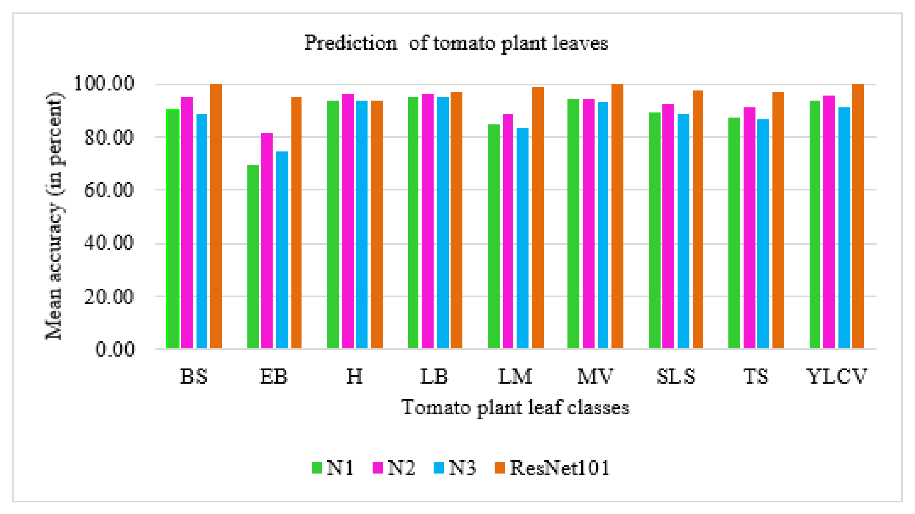
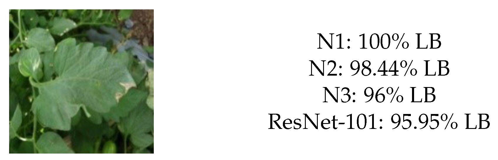
- To validate the versatility of the proposed models, they were also employed in tomato leaf disease classification using images captured from a mobile phone. The disease classification accuracy shows that the proposed models are well suited for TPL disease classification.
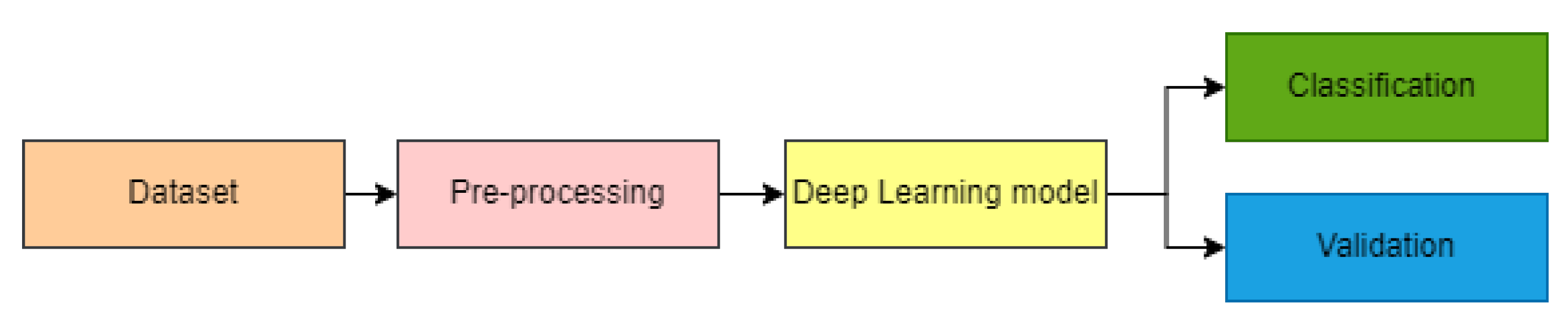
2. Materials and Methods
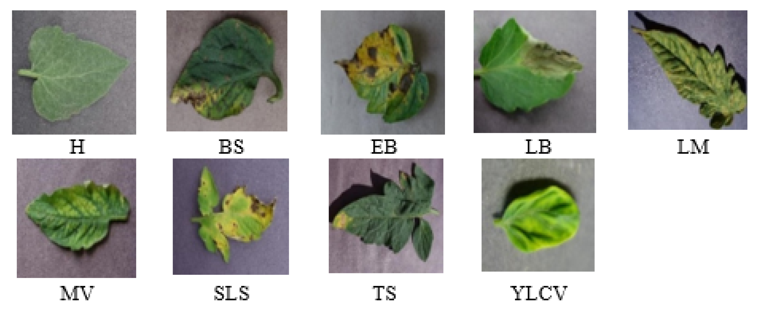
2.1. Dataset and Pre-Processing
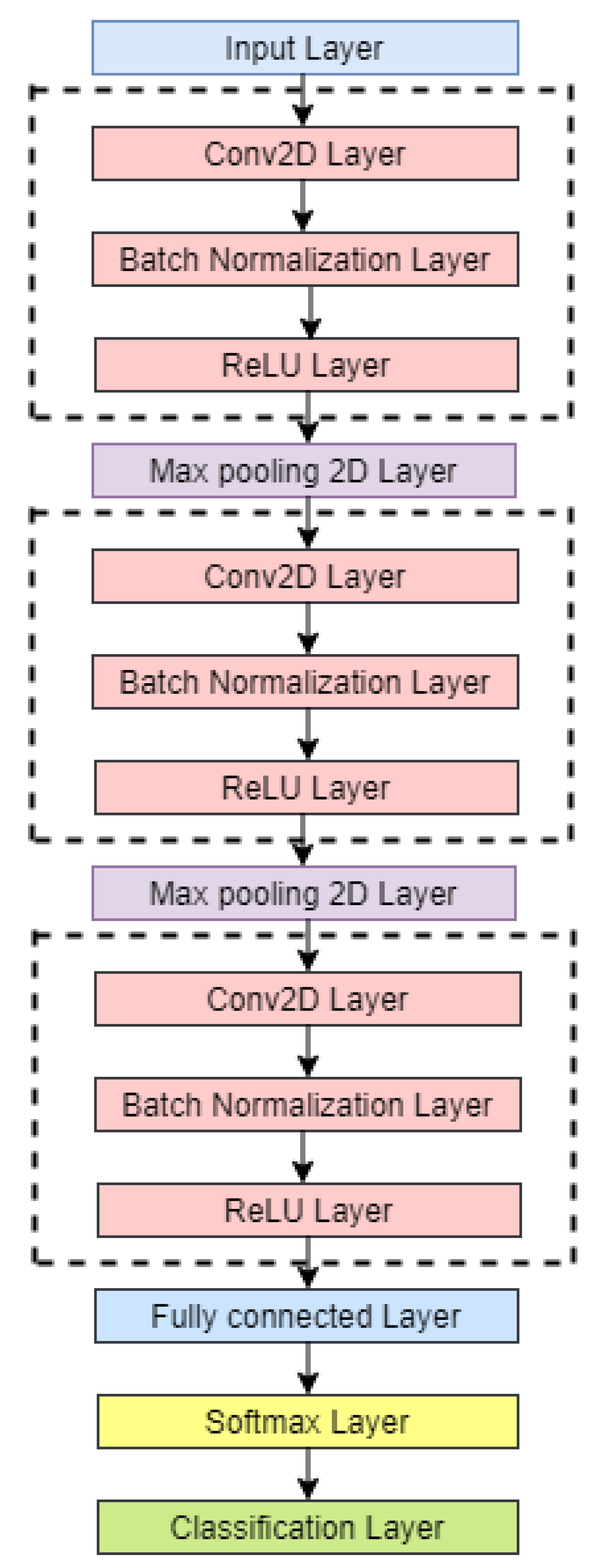
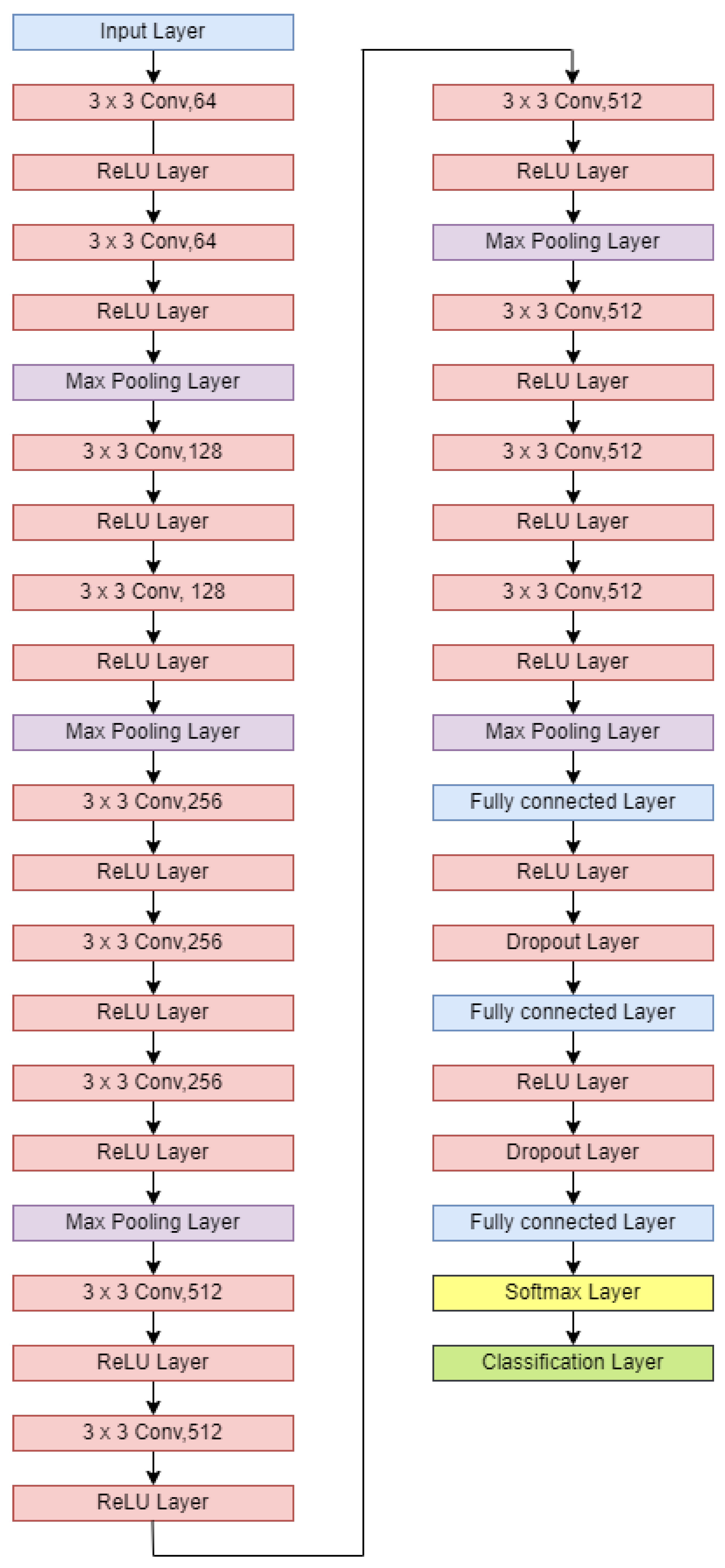
2.2. CNN Models
2.3. The CNN Model
- “True positives (TP) represent the positive samples that were correctly labeled by the classifier,”
- “True negatives (TN) represent the negative samples correctly labeled by the classifier,”
- “False positives (FP) represent the negative samples incorrectly labeled as positive,” and
- “False negatives (FN) correctly labeled the positive samples incorrectly labeled as negative.”
2.4. Validation of the Trained CNN Model
3. Results and Discussion
4. Conclusions
Author Contributions
Funding
Acknowledgments
Conflicts of Interest
References
- AlZu’bi, S.; Hawashin, B.; Mujahed, M.; Jararweh, Y.; Gupta, B.B. An efficient employment of internet of multimedia things in smart and future agriculture. Multimed. Tools Appl. 2019, 78, 29581–29605. [Google Scholar] [CrossRef]
- Arivazhagan, S.; Shebiah, R.N.; Ananthi, S.; Varthini, S.V. Detection of unhealthy region of plant leaves and classification of plant leaf diseases using texture features. Agric. Eng. Int. CIGR J. 2013, 15, 211–217. [Google Scholar]
- Al Bashish, D.; Braik, M.; Bani-ahmad, S. A Framework for Detection and Classification of Plant Leaf and Stem Diseases. In Proceedings of the International Conference on Signal and Image Processing, Chennai, India, 15–17 December 2010; pp. 113–118. [Google Scholar]
- Ferentinos, K.P. Deep learning models for plant disease detection and diagnosis. Comput. Electron. Agric. 2018, 145, 311–318. [Google Scholar] [CrossRef]
- Lee, S.H.; Chan, C.S.; Mayo, S.J.; Remagnino, P. How deep learning extracts and learns leaf features for plant classification. Pattern Recognit. 2017, 71, 1–13. [Google Scholar] [CrossRef]
- Kumar, N.; Belhumeur, P.N.; Biswas, A.; Jacobs, D.W.; Kress, W.J.; Lopez, I.C.; Soares, J.V. Leafsnap: A Computer Vision System for Automatic Plant Species Identification. In Proceedings of the European Conference on Computer Vision, Firenze, Italy, 7–13 October 2012; pp. 502–516. [Google Scholar] [CrossRef]
- Yann, L.; Leon, B.; Yoshua, B.; Patrick, H. Gradient-Based Learning Applied to Document Recognition. Proc. IEEE 1998, 86, 2278–2324. [Google Scholar] [CrossRef]
- Aquil, M.A.I.; Ishak, W.H.W. Evaluation of scratch and pre-trained convolutional neural networks for the classification of tomato plant diseases. IAES Int. J. Artif. Intell. 2021, 10, 467–475. [Google Scholar] [CrossRef]
- Schmidt, K.W.; Hazir, O. A Data Envelopment Analysis Method for Finding Robust and Cost-Efficient Schedules in Multimode Projects. IEEE Trans. Eng. Manag. 2019, 67, 414–429. [Google Scholar] [CrossRef]
- Elmousalami, H.H. Comparison of artificial intelligence techniques for project conceptual cost prediction. IEEE Trans. Eng. Manag. 2020, 68, 183–196. [Google Scholar] [CrossRef]
- He, K.; Zhang, X.; Ren, S.; Sun, J. Deep residual learning for image recognition. In Proceedings of the IEEE Conference on Computer Vision and Pattern Recognition, Las Vegas, NV, USA, 27–30 June 2016; pp. 770–778. [Google Scholar] [CrossRef]
- Raghu, S.; Sriraam, N.; Temel, Y.; Rao, S.V.; Kubben, P.L. EEG based multi-class seizure type classification using convolutional neural network and transfer learning. Neural Netw. 2020, 124, 202–212. [Google Scholar] [CrossRef]
- Syarief, M.; Setiawan, W. Convolutional neural network for maize leaf disease image classification. Telkomnika Telecommun. Comput. Electron. Control 2020, 18, 1376–1381. [Google Scholar] [CrossRef]
- Hu, X.; Xu, J.; Wu, J. A Novel Electronic Component Classification Algorithm Based on Hierarchical Convolution Neural Network. In Proceedings of the IOP Conference Series: Earth and Environmental Science, Changsha, China, 18–20 September 2020; Volume 474, pp. 1–7. [Google Scholar] [CrossRef]
- Al-Qerem, A.; Alauthman, M.; Almomani, A.; Gupta, B.B. IoT transaction processing through cooperative concurrency control on fog–cloud computing environment. Soft Comput. 2020, 24, 5695–5711. [Google Scholar] [CrossRef]
- Abid, A.; Sinha, P.; Harpale, A.; Gichoya, J.; Purkayastha, S. Distributed Computing and Artificial Intelligence—9th International Conference. In Optimizing Medical Image Classification Models for Edge Devices; AISC: Springer, Berlin, Germany, 2021; Volume 151, pp. 77–87. [Google Scholar]
- Rangarajan, A.K.; Purushothaman, R. Tomato crop disease classification using pre-trained deep learning algorithm. In Proceedings of the International Conference on Robotics and Smart Manufacturing, Chennai, India, 19–21 July 2018; Volume 133, pp. 1040–1047. [Google Scholar] [CrossRef]
- Fuentes, A.; Yoon, S.; Kim, S.C.; Park, D.S. A Robust Deep-Learning-Based Detector for Real-Time Tomato Plant Diseases and Pests Recognition. Sensors 2017, 17, 2022. [Google Scholar] [CrossRef]
- Fuentes, A.F.; Yoon, S.; Lee, J.; Park, D.S. High-Performance Deep Neural Network-Based Tomato Plant Diseases and Pests Diagnosis System With Refinement Filter Bank. Front. Plant Sci. 2018, 9, 1162. [Google Scholar] [CrossRef]
- Duan, C.Y.; Chen, X.Q.; Shi, H.; Liu, H.C. A New Model for Failure Mode and Effects Analysis Based on k-Means Clustering Within Hesitant Linguistic Environment. IEEE Trans. Eng. Manag. 2019, 69, 1837–1847. [Google Scholar] [CrossRef]
- Hasan, R.I.; Yusuf, S.M.; Alzubaidi, L. Review of the state of the art of deep learning for plant diseases: A broad analysis and discussion. Plants 2020, 9, 1302. [Google Scholar] [CrossRef]
- Liu, J.; Yang, S.; Cheng, Y.; Song, Z. Plant Leaf Classification Based on Deep Learning. In Proceedings of the 2018 Chinese Automation Congress (CAC), Xi’an, China, 30 November–2 December 2019; pp. 3165–3169. [Google Scholar] [CrossRef]
- Mukti, I.Z.; Biswas, D. Transfer Learning Based Plant Diseases Detection Using ResNet50. In Proceedings of the 2019 4th International Conference on Electrical Information and Communication Technology, EICT 2019, Khulna, Bangladesh, 20–22 December 2019; pp. 1–6. [Google Scholar] [CrossRef]
- Wagle, S.A.; Harikrishnan, R. Comparison of Plant Leaf Classification Using Modified AlexNet and Support Vector Machine. Traitement Signal 2021, 38, 79–87. [Google Scholar] [CrossRef]
- Jadhav, S.B.; Udupi, V.R.; Patil, S.B. Convolutional neural networks for leaf image-based plant disease classification. IAES Int. J. Artif. Intell. 2019, 8, 328–341. [Google Scholar] [CrossRef]
- Chen, J.; Chen, J.; Zhang, D.; Sun, Y.; Nanehkaran, Y.A. Using deep transfer learning for image-based plant disease identification. Comput. Electron. Agric. 2020, 173, 105393. [Google Scholar] [CrossRef]
- Islam, M.A.; Shuvo, N.R.; Shamsojjaman, M.; Hasan, S.; Hossain, S.; Khatun, T. An Automated Convolutional Neural Network Based Approach for Paddy Leaf Disease Detection. Int. J. Adv. Comput. Sci. Appl. 2021, 12, 280–288. [Google Scholar] [CrossRef]
- Bari, B.S.; Islam, M.N.; Rashid, M.; Hasan, M.J.; Razman, M.A.M.; Musa, R.M.; Ab Nasir, A.F.; Majeed, A.P.A. A real-time approach of diagnosing rice leaf disease using deep learning-based faster R-CNN framework. PeerJ Comput. Sci. 2021, 7, e432. [Google Scholar] [CrossRef]
- Rangarajan Aravind, K.; Raja, P. Automated disease classification in (Selected) agricultural crops using transfer learning. Automatika 2020, 61, 260–272. [Google Scholar] [CrossRef]
- Begum, A.S.; Savitha, S.; Shahila, S.; Sharmila, S. Diagnosis of Leaf Disease Using Enhanced Convolutional Neural Network. Int. J. Innov. Res. Appl. Sci. Eng. 2020, 3, 579–586. [Google Scholar] [CrossRef]
- Wang, Q.; Qi, F. Tomato diseases recognition based on faster RCNN. In Proceedings of the 10th International Conference on Information Technology in Medicine and Education, ITME 2019, Qingdao, China, 23–25 August 2019; pp. 772–776. [Google Scholar] [CrossRef]
- Li, W.; Liu, H.; Wang, Y.; Li, Z.; Jia, Y.; Gui, G. Deep Learning-Based Classification Methods for Remote Sensing Images in Urban Built-Up Areas. IEEE Access 2019, 7, 36274–36284. [Google Scholar] [CrossRef]
- Brahimi, M.; Boukhalfa, K.; Moussaoui, A. Deep Learning for Tomato Diseases: Classification and Symptoms Visualization. Appl. Artif. Intell. 2017, 31, 299–315. [Google Scholar] [CrossRef]
- Zhang, K.; Wu, Q.; Liu, A.; Meng, X. Can deep learning identify tomato leaf disease? Adv. Multimed. 2018, 2018, 6710865. [Google Scholar] [CrossRef]
- Karthik, R.; Hariharan, M.; Anand, S.; Mathikshara, P.; Johnson, A.; Menaka, R. Attention embedded residual CNN for disease detection in tomato leaves. Appl. Soft Comput. J. 2020, 86, 105933. [Google Scholar] [CrossRef]
- Gonzalez-Huitron, V.; León-Borges, J.A.; Rodriguez-Mata, A.E.; Amabilis-Sosa, L.E.; Ramírez-Pereda, B.; Rodriguez, H. Disease detection in tomato leaves via CNN with lightweight architectures implemented in Raspberry Pi 4. Comput. Electron. Agric. 2021, 181, 105951. [Google Scholar] [CrossRef]
- Mohanty, S.P.; Hughes, D.P.; Salathé, M. Using Deep Learning for Image-Based Plant Disease Detection. Front. Plant Sci. 2016, 7, 1419. [Google Scholar] [CrossRef]
- Dyrmann, M.; Karstoft, H.; Midtiby, H.S. Plant species classification using deep convolutional neural network. Biosyst. Eng. 2016, 151, 72–80. [Google Scholar] [CrossRef]
- Zhang, Y.; Phillips, P.; Wang, S.; Ji, G.; Yang, J.; Wu, J. Fruit classification by biogeography-based optimization and feedforward neural network. Expert Syst. 2016, 33, 239–253. [Google Scholar] [CrossRef]
- Zhang, Y.D.; Satapathy, S.C.; Wang, S.H. Fruit category classification by fractional Fourier entropy with rotation angle vector grid and stacked sparse autoencoder. Expert Syst. 2021, 39, e12701. [Google Scholar] [CrossRef]
- Wagle, S.A.; Harikrishnan, R.; Md Ali, S.H.; Mohammad, F. Classification of Leaves Using New Compact Convolutional Neural Network Models. Plants 2022, 11, 24. [Google Scholar] [CrossRef] [PubMed]
- Garbin, C.; Zhu, X.; Marques, O. Dropout vs. batch normalization: An empirical study of their impact to deep learning. Multimed. Tools Appl. 2020, 79, 12777–12815. [Google Scholar] [CrossRef]
- Jaiswal, S.; Nandi, G.C. Robust real-time emotion detection system using CNN architecture. Neural Comput. Appl. 2020, 32, 11253–11262. [Google Scholar] [CrossRef]
- Längkvist, M.; Jendeberg, J.; Thunberg, P.; Loutfi, A.; Lidén, M. Computer aided detection of ureteral stones in thin slice computed tomography volumes using Convolutional Neural Networks. Comput. Biol. Med. 2018, 97, 153–160. [Google Scholar] [CrossRef] [PubMed]
- Simonyan, K.; Zisserman, A. Very deep convolutional networks for large-scale image recognition. In Proceedings of the 3rd International Conference on Learning Representations, ICLR 2015, San Diego, CA, USA, 7–9 May 2015; pp. 1–14. [Google Scholar]
- Sathyanarayana, A.; Joty, S.; Fernandez-Luque, L.; Ofli, F.; Srivastava, J.; Elmagarmid, A.; Arora, T.; Taheri, S. Sleep Quality Prediction From Wearable Data Using Deep Learning. JMIR mHealth uHealth 2016, 4, e6562. [Google Scholar]
- Heydarian, M.; Doyle, T.E.; Samavi, R. MLCM: Multi-Label Confusion Matrix. IEEE Access 2022, 10, 19083–19095. [Google Scholar] [CrossRef]
- Moradi, R.; Berangi, R.; Minaei, B. A survey of regularization strategies for deep models. Artif. Intell. Rev. 2020, 53, 3947–3986. [Google Scholar] [CrossRef]
- Shorten, C.; Khoshgoftaar, T.M. A survey on Image Data Augmentation for Deep Learning. J. Big Data 2019, 6, 60. [Google Scholar] [CrossRef]
- Anandhakrishnan, T.; Jaisakthi, S.M. Identification of tomato leaf disease detection using pretrained deep convolutional neural network models. Scalable Comput. 2020, 21, 625–635. [Google Scholar] [CrossRef]
- Deep Learning, MATLAB2019b. Available online: https://in.mathworks.com (accessed on 30 April 2021).
- Qiu, W.; Ye, J.; Hu, L.; Yang, J.; Li, Q.; Mo, J.; Yi, W. Distilled-mobilenet model of convolutional neural network simplified structure for plant disease recognition. Smart Agric. 2021, 3, 109–117. [Google Scholar] [CrossRef]
- Awan, M.J.; Rahim, M.S.M.; Salim, N.; Rehman, A.; Nobanee, H.; Shabir, H. Improved Deep Convolutional Neural Network to Classify Osteoarthritis from Anterior Cruciate Ligament Tear Using Magnetic Resonance Imaging. J. Pers. Med. 2021, 11, 1163. [Google Scholar] [CrossRef] [PubMed]
- Durante, M.G.; Rathje, E.M. An exploration of the use of machine learning to predict lateral spreading. Earthq. Spectra 2021, 37, 2288–2314. [Google Scholar] [CrossRef]


| Ref No | Model | Objective | Dataset | Accuracy | Limitations |
|---|---|---|---|---|---|
| [22] | Ten-layer CNN | Classification of plant leaf | Flavia | 87.92% | Flavia dataset consists of only healthy classes. Diseased classes are not studied. |
| [23] | AlexNet VGG19 VGG16 ResNet-50 | Identification of plant disease | PlantVillage | 83.66% 91.75% 94.96% 99.8% | Plant disease detection models can be deployed in mobile to help the farmers. |
| [26] | INC-VGGN | Classification of rice plant images | PlantVillage Own dataset | 84.25% 91.83% | The size of the developed model is more to be used directly to be deployed on mobile as an App |
| [27] | ResNet-101 | Classification of paddy leaf disease | Kaggle and UCI repository | 91.52% | Other variety of paddy leaf diseases with a larger dataset and other CNN models can be used for better accuracy |
| [28] | Faster R-CNN | Diagnosis of rice plant disease | Kaggle and own dataset | 98.25% | A mobile-based system with IoT can be implemented for future work. |
| [25] | AlexNet GoogLeNet VGG16 ResNet-101 DenseNet 201 | Classification of soyabean plant disease | PlantVillage | 95% 96.4% 96.4% 92.1% 93.6% | To develop a CNN model for better classification accuracy |
| [30] | Xception Inception Resnet-V2 MobileNetV2 | Classification of plant disease | PlantVillage | 94% 95% 97% | More classes can be used for the classification problem. |
| [29] | ResNet-101 GoogLeNet | Classification of ten different diseases in four crops | Own dataset | 96.9% 97.3% | Dataset with a complex background can be used for classification. |
| [33] | AlexNet GoogLeNet | Classification of tomato plant disease | PlantVillage | 98.66% 99.18% | The computation and size of the classification model can be reduced. |
| [17] | AlexNet VGG16 | Classification of tomato plant disease | PlantVillage | 97.49% 97.29% | The VGG16 model is computationally intensive. |
| [34] | ResNet-50 | Identifying tomato leaf disease | PlantVillage | 97.28% | The classification model can be used for detecting more variety of disease classes. |
| [35] | Attention-based Residual CNN | Detection of tomato leaf disease | PlantVillage | 98% | More disease classes can be used in the future to detect disease. |
| [36] | MobileNetV2 NasNetMobile Xception MobileNetV3 | Disease detection in tomato plant leaves | PlantVillage | 75% 84% 100% 98% | Xception model is performing as the best classifier with high computation cost. |
| Class | PV Database | |
|---|---|---|
| Before Augmentation | After Augmentation | |
| “BS” | 100 | 10,500 |
| “EB” | 100 | 10,500 |
| “H” | 100 | 10,500 |
| “LB” | 100 | 10,500 |
| “LM” | 100 | 10,500 |
| “MV” | 100 | 10,500 |
| “SLS” | 100 | 10,500 |
| “TS” | 100 | 10,500 |
| “YLCV” | 100 | 10,500 |
| TOTAL | 900 | 94,500 |
| CNN Layer | CNN Model | ||
|---|---|---|---|
| N1 | N2 | N3 | |
| 1st Conv2D | 3 × 3, 8 | 3 × 3, 16 | 7 × 7, 8 |
| 2nd Conv2D | 3 × 3, 16 | 3 × 3, 32 | 5 × 5, 16 |
| 3rd Conv2D | 3 × 3, 32 | 3 × 3, 64 | 3 × 3, 32 |
| Model & Ref No. | Datasize | Accuracy | Model Size |
|---|---|---|---|
| AlexNet [33] | 14,828 | 98.66% | 227 MB [51] |
| GoogLeNet [33] | 14,828 | 99.18% | 27 MB [51] |
| AlexNet [17] | 13,262 | 97.49% | 227 MB [51] |
| VGG16 [17] | 13,262 | 97.29% | 515 MB [51] |
| ResNet [34] | 41,127 | 97.28% | 96 MB [51] |
| Ten-layer CNN [22] | 94,500 | 84.02% | 7 MB |
| Attention based Residual CNN [35] | 95,999 | 98% | Not given |
| Xception V4 [50] | 14,528 | 99.45% | 85 MB [51] |
| Distilled MobileNet [52] | 54,305 | 97.62% | 19.83 MB |
| VGG16 | 94,500 | 99.21% | 477 MB |
| N1 | 94,500 | 99.13% | 8.5 MB |
| N2 | 94,500 | 99.51% | 17.14 MB |
| N3 | 94,500 | 99.40% | 8.5 MB |
| ResNet-101 | 94,500 | 99.97% | 151 MB |
| (a)“Confusion matrix for ResNet-101 model.” | ||||||||||
| Actual Class | ||||||||||
| Predicted Class | Class | BS | EB | H | LB | LM | MV | SLS | TS | YLCV |
| BS | 2097 | 0 | 0 | 0 | 0 | 0 | 1 | 0 | 2 | |
| EB | 0 | 2100 | 0 | 0 | 0 | 0 | 0 | 0 | 0 | |
| H | 0 | 0 | 2100 | 0 | 0 | 0 | 0 | 0 | 0 | |
| LB | 0 | 0 | 0 | 2099 | 0 | 0 | 1 | 0 | 0 | |
| LB | 0 | 0 | 0 | 0 | 2100 | 0 | 0 | 0 | 0 | |
| MV | 0 | 0 | 0 | 0 | 0 | 2100 | 0 | 0 | 0 | |
| SLS | 0 | 0 | 0 | 0 | 0 | 0 | 2100 | 0 | 0 | |
| TS | 0 | 0 | 2 | 0 | 0 | 0 | 0 | 2098 | 0 | |
| YLCV | 0 | 0 | 0 | 0 | 0 | 0 | 0 | 0 | 2100 | |
| (b)Confusion matrix for N1 model | ||||||||||
| Actual Class | ||||||||||
| Predicted Class | Class | BS | EB | H | LB | LM | MV | SLS | TS | YLCV |
| BS | 2077 | 4 | 0 | 3 | 0 | 0 | 13 | 3 | 0 | |
| EB | 0 | 2064 | 1 | 6 | 5 | 0 | 19 | 3 | 2 | |
| H | 0 | 0 | 2100 | 0 | 0 | 0 | 0 | 0 | 0 | |
| LB | 0 | 0 | 0 | 2094 | 0 | 1 | 2 | 0 | 3 | |
| LB | 2 | 2 | 0 | 2 | 2078 | 2 | 6 | 7 | 1 | |
| MV | 0 | 0 | 3 | 3 | 0 | 2090 | 4 | 0 | 0 | |
| SLS | 4 | 0 | 0 | 11 | 2 | 0 | 2083 | 0 | 0 | |
| TS | 0 | 0 | 1 | 0 | 0 | 0 | 4 | 2095 | 0 | |
| YLCV | 4 | 5 | 0 | 9 | 2 | 3 | 16 | 7 | 2054 | |
| (c)Confusion matrix for N2 model | ||||||||||
| Actual Class | ||||||||||
| Predicted Class | Class | BS | EB | H | LB | LM | MV | SLS | TS | YLCV |
| BS | 2080 | 4 | 0 | 1 | 3 | 0 | 6 | 0 | 6 | |
| EB | 0 | 2097 | 0 | 1 | 0 | 0 | 1 | 1 | 0 | |
| H | 0 | 0 | 2097 | 2 | 0 | 0 | 1 | 0 | 0 | |
| LB | 0 | 0 | 1 | 2076 | 6 | 2 | 6 | 1 | 8 | |
| LB | 1 | 2 | 0 | 2 | 2074 | 0 | 11 | 0 | 10 | |
| MV | 0 | 0 | 0 | 0 | 0 | 2095 | 4 | 0 | 1 | |
| SLS | 2 | 0 | 0 | 1 | 0 | 2 | 2092 | 0 | 3 | |
| TS | 0 | 0 | 1 | 0 | 0 | 0 | 1 | 2098 | 0 | |
| YLCV | 0 | 0 | 0 | 1 | 1 | 0 | 0 | 0 | 2098 | |
| (d)Confusion matrix for N3 model | ||||||||||
| Actual Class | ||||||||||
| Predicted Class | Class | BS | EB | H | LB | LM | MV | SLS | TS | YLCV |
| BS | 2074 | 3 | 0 | 3 | 4 | 1 | 8 | 2 | 5 | |
| EB | 2 | 2090 | 0 | 3 | 1 | 1 | 1 | 1 | 1 | |
| H | 0 | 0 | 2099 | 1 | 0 | 0 | 0 | 0 | 0 | |
| LB | 0 | 2 | 2 | 2090 | 0 | 1 | 3 | 0 | 2 | |
| LB | 2 | 2 | 0 | 7 | 2080 | 2 | 7 | 0 | 0 | |
| MV | 0 | 0 | 0 | 0 | 0 | 2096 | 4 | 0 | 0 | |
| SLS | 0 | 1 | 1 | 5 | 4 | 2 | 2083 | 1 | 3 | |
| TS | 0 | 0 | 3 | 0 | 0 | 0 | 0 | 2097 | 0 | |
| YLCV | 1 | 2 | 2 | 5 | 2 | 6 | 3 | 1 | 2078 | |
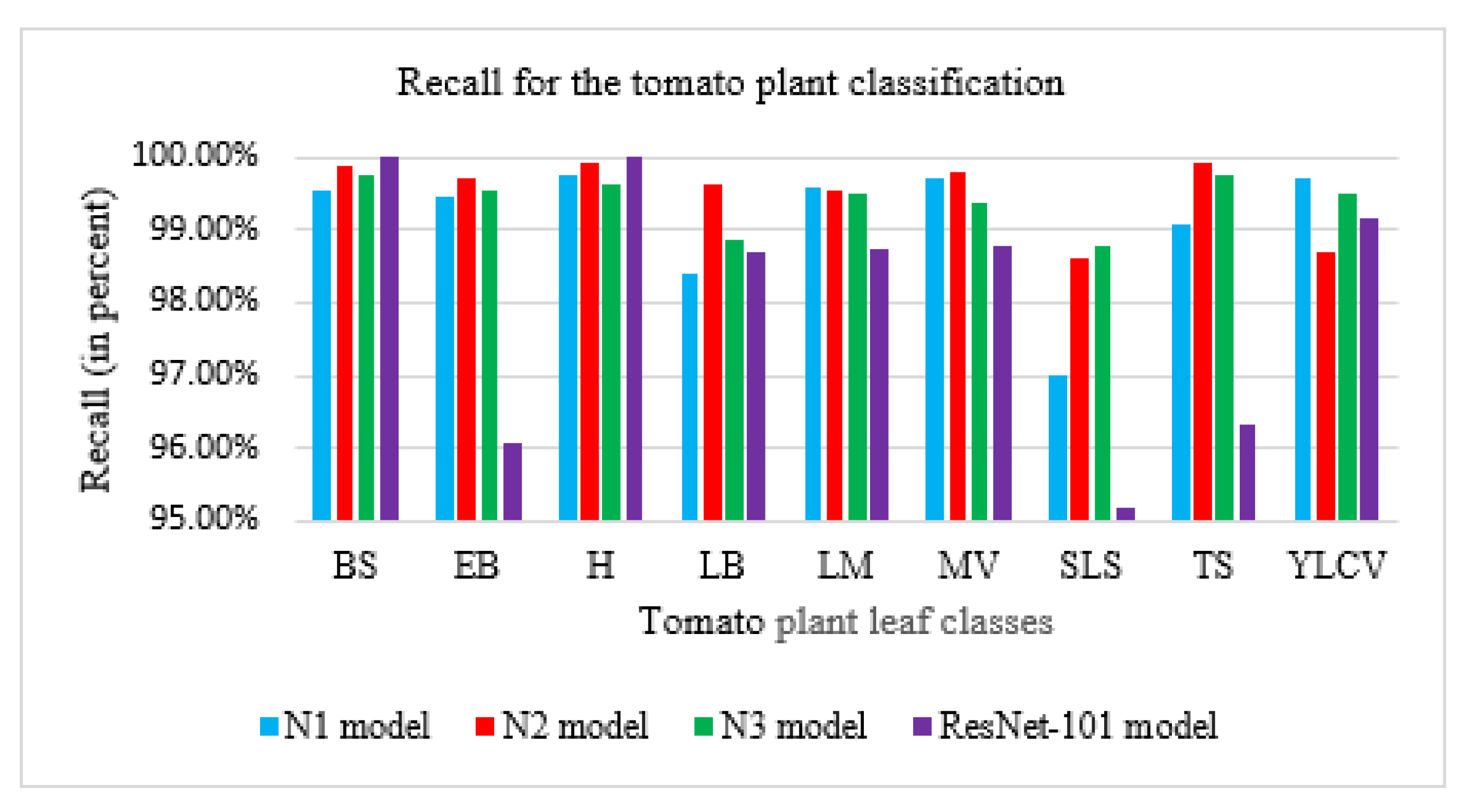
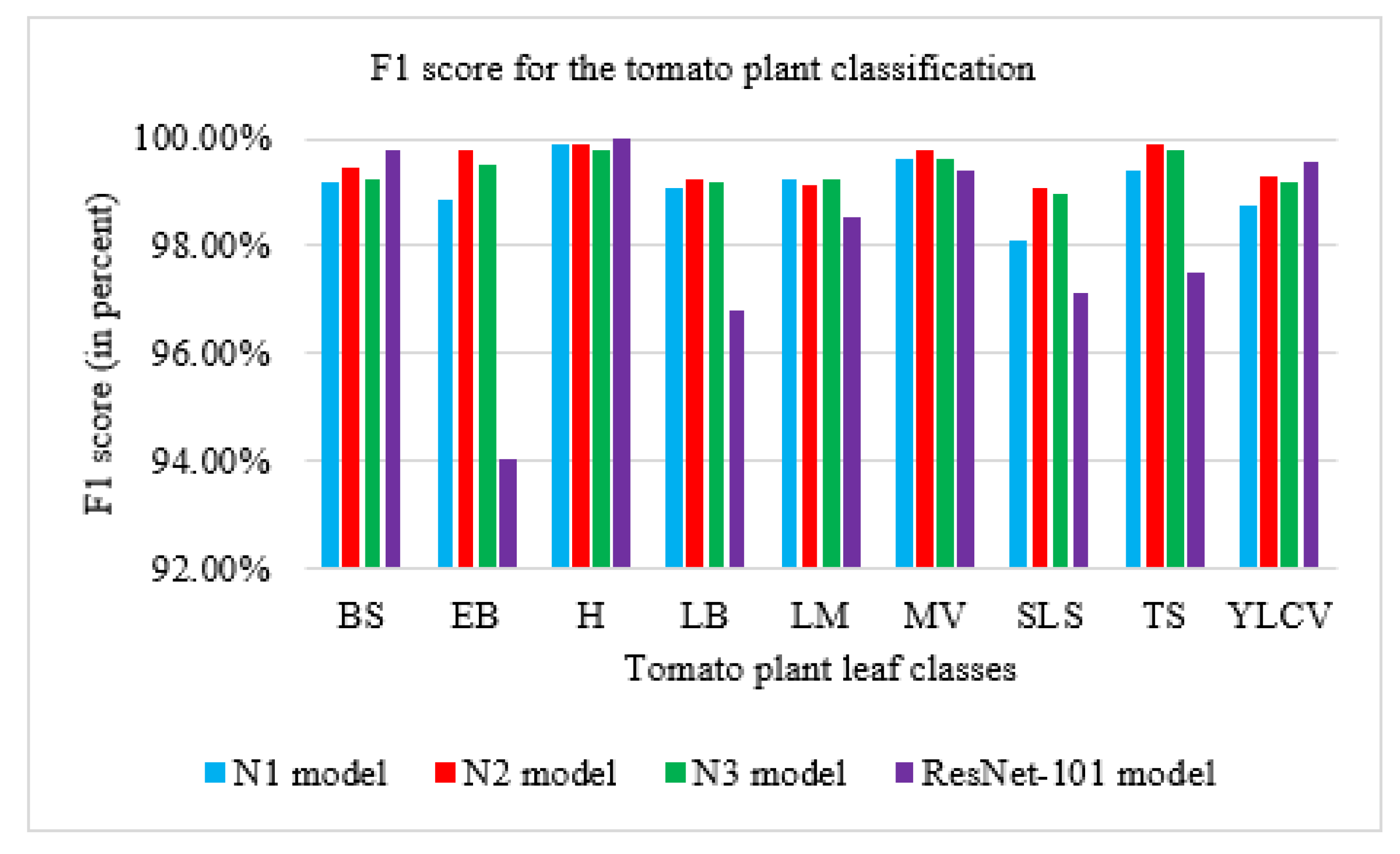
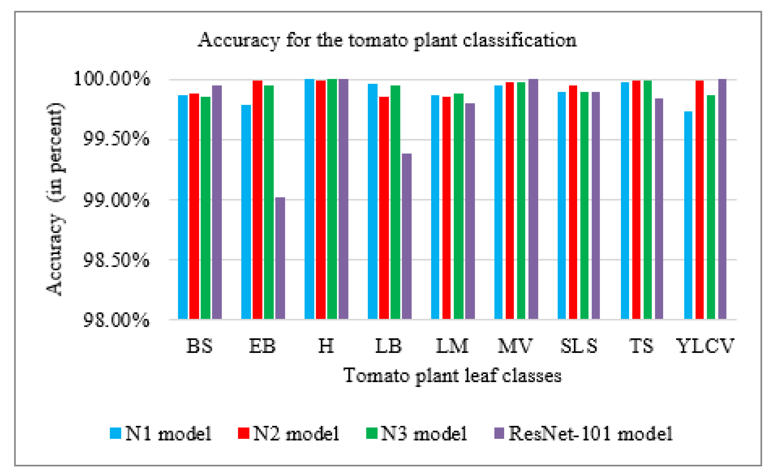
| “Model” | “Macro Recall” | “Macro Precision” | “Macro F1 Score” | “Mean Accuracy” |
|---|---|---|---|---|
| N1 | 99.13% | 99.13% | 99.13% | 99.81% |
| N2 | 99.51% | 99.51% | 99.51% | 99.89% |
| N3 | 99.4% | 99.4% | 99.4% | 99.86% |
| ResNet-101 | 98.11% | 98.1% | 98.09% | 99.58% |
| Class | N1 | N2 | N3 | ResNet-101 |
|---|---|---|---|---|
| BS | 98.9% | 99.05% | 98.76% | 99.58% |
| EB | 98.29% | 99.86% | 99.52% | 92.08% |
| H | 100% | 99.86% | 99.95% | 100% |
| LB | 99.71% | 98.86% | 99.52% | 95% |
| LM | 98.95% | 98.76% | 99.05% | 98.33% |
| MV | 99.52% | 99.76% | 99.81% | 100% |
| SLS | 99.19% | 99.62% | 99.19% | 99.17% |
| TS | 99.76% | 99.9% | 99.86% | 98.75% |
| YLCV | 97.81% | 99.9% | 98.95% | 100% |
Publisher’s Note: MDPI stays neutral with regard to jurisdictional claims in published maps and institutional affiliations. |
© 2022 by the authors. Licensee MDPI, Basel, Switzerland. This article is an open access article distributed under the terms and conditions of the Creative Commons Attribution (CC BY) license (https://creativecommons.org/licenses/by/4.0/).
Share and Cite
Wagle, S.A.; R, H.; Varadarajan, V.; Kotecha, K. A New Compact Method Based on a Convolutional Neural Network for Classification and Validation of Tomato Plant Disease. Electronics 2022, 11, 2994. https://doi.org/10.3390/electronics11192994
Wagle SA, R H, Varadarajan V, Kotecha K. A New Compact Method Based on a Convolutional Neural Network for Classification and Validation of Tomato Plant Disease. Electronics. 2022; 11(19):2994. https://doi.org/10.3390/electronics11192994
Chicago/Turabian StyleWagle, Shivali Amit, Harikrishnan R, Vijayakumar Varadarajan, and Ketan Kotecha. 2022. "A New Compact Method Based on a Convolutional Neural Network for Classification and Validation of Tomato Plant Disease" Electronics 11, no. 19: 2994. https://doi.org/10.3390/electronics11192994