Intelligent Identification and Order-Sensitive Correction Method of Outliers from Multi-Data Source Based on Historical Data Mining

Abstract

In recent years, outliers caused by manual operation errors and equipment acquisition failures often occur, bringing challenges to big data analysis. In view of the difficulties in identifying and correcting outliers of multi-source data, an intelligent identification and order-sensitive correction method of outliers from multi-data sources based on historical data mining was proposed. First, an intelligent identification method of outliers of single-source data is proposed based on neural tangent kernel K-means (NTKKM) clustering. The original data is mapped to high-dimensional feature space using Neural Tangent Kernel, where the features of outliers are acquired by K-means clustering to realize the accurate identification of outliers. Second, an order-sensitive missing value imputation framework for multi-source data (OMSMVI) was proposed. The similarity graph of sources with missing data was constructed based on multidimensional similarity analysis, and the filling order decision was transformed into an optimization problem to realize the optimal filling order decision of missing values in multi-source data. Finally, a neighborhood-based imputation (NI) algorithm is proposed. Based on the traditional KNN filling algorithm, neighboring nodes of sources with missing data are flexibly selected to the achieve accurate correction of outliers. The case experiment was operated on actual power grid data, and the results show that the proposed clustering method can identify outliers more accurately, and the determined optimal imputation sequence has higher accuracy, which provide a feasible new idea for the identification and correction of outliers in the process of data preprocessing.

1. Introduction

With the development of sensor and perception network technology, a large number of multi-source data are produced in practical engineering projects, such as temperature, humidity, air quality and other meteorological data, with voltage, power and phase data monitored by SCADA (Supervisory Control and Data Acquisition) and PMU (Phasor Measurement Unit) in power systems. In the era of big data, data has become an important reference in technological innovation, industrial development and other fields, and the process of data collection and pre-processing has received increasing attention. Abnormal monitoring data is an inevitable problem in the process of multi-source data collection and transmission. There are various reasons for the occurrence of abnormal data, including sensor equipment failure, communication interruption, manual operation error and so on [1,2]. Most of the existing data mining analysis algorithm is based on high quality data sets, and abnormal data will reduce the sample information, improving the complexity of data analysis. If the abnormal data are not handled or improperly handled, existing analyses method will be unable to dig out the useful information or even dig out error messages [3]. Therefore, how to process abnormal data correctly and efficiently becomes one of the key issues in data analysis [4,5,6].

There are two main methods to deal with abnormal data: the delete method and fill method. The delete method directly deletes abnormal data of the data set, which loses the opportunity to discover effective implicit information, leading to huge losses. The fill method is to select an appropriate value to replace the abnormal part of the data set, so as to form a complete data set. This method needs to ensure the accuracy of filling data and avoid distortion as far as possible. In terms of the identification of outliers from multi-source data, the literature [7] first combined the improved DBSCAN algorithm with compound time-series similarity measure criteria to realize outlier identification of the multi-source IoT power distribution monitoring terminal, then using the spatial correlation of the data from the terminal unit, extracting the collection features of the spatial correlation coefficient of the terminal node to realize the precise recognition of the monitoring terminal with abnormal data. Based on the feature analysis of outliers of multi-source data, the literature [8] proposed an outlier measurement method of the deep fusion method of KNN-RNN and introduced the KNN-Join optimization operator to accelerate the execution speed of the algorithm and realize fast recognition of outliers of multi-source data. In terms of the correction of outliers from multi-source data, the literature [9] proposed an abnormal data processing method based on the stack de-noising automatic encoder and multi-sensor cooperation, to solve problems processing outliers of multi-source data in wireless sensor networks. The abnormal data are distinguished via multi-sensor collaboration, and the stack de-noising automatic encoder was used to realize data cleaning. The literature [10] proposed a multi-source missing data and abnormal data correction framework based on the generalized addition and auto-regression model, to solve the problem of multi-source data missing and abnormal data processing in aquatic environmental monitoring, which effectively assisted the monitoring and management of freshwater eco systems. According to the spatial distribution characteristics of abnormal and normal data pixels in wind power curve images, the literature [11] extracted abnormal and normal data pixels through image processing to achieve rapid cleaning of abnormal data of wind turbines.

Based on the correlation of time and attributes of multi-source data, an intelligent identification and order-sensitive correction method of outliers from multi-data source based on historical data mining was proposed. Firstly, an intelligent identification method of outliers of single-source data is proposed based on the Neural Tangent Kernel K-means (NTKKM) clustering algorithm. Input data space is mapped to high-dimensional feature space through Neural Tangent Kernel. Then, in the high-dimensional feature space, abnormal data features are mined by K-means clustering, which are identified and deleted for subsequent filling operations. Secondly, for the filling problem of multiple densely distributed missing data, an order-sensitive missing value imputation framework for multi-source sensory data (OMSMVI) was proposed. Considering that the filled missing values are used as reference values for subsequent filling, the filling order decision problem is transformed into an optimization problem to decide the optimal filling order of missing values in multi-source data. Finally, aiming at the problem that the K value of the traditional KNN filling algorithm is difficult to determine, a Neighborhood-based Imputation (NI) algorithm is proposed to improve the traditional KNN filling algorithm. Using the multidimensional similarity of multi-source data to find all the neighbors of the missing data source, the nearest neighbor nodes suitable for filling was found, and the missing data can be filled, and the abnormal data can be corrected. An example of actual power grid data of a China city is set as the experimental object. We compared the proposed clustering and missing data filling algorithm with the traditional method. The results show that the proposed clustering method can realize the effective partition of abnormal data more accurately compared with the traditional clustering algorithm, and the determined optimal filling sequence has higher accuracy. The proposed method provides a feasible new idea for the identification and correction of abnormal data in the process of data preprocessing.

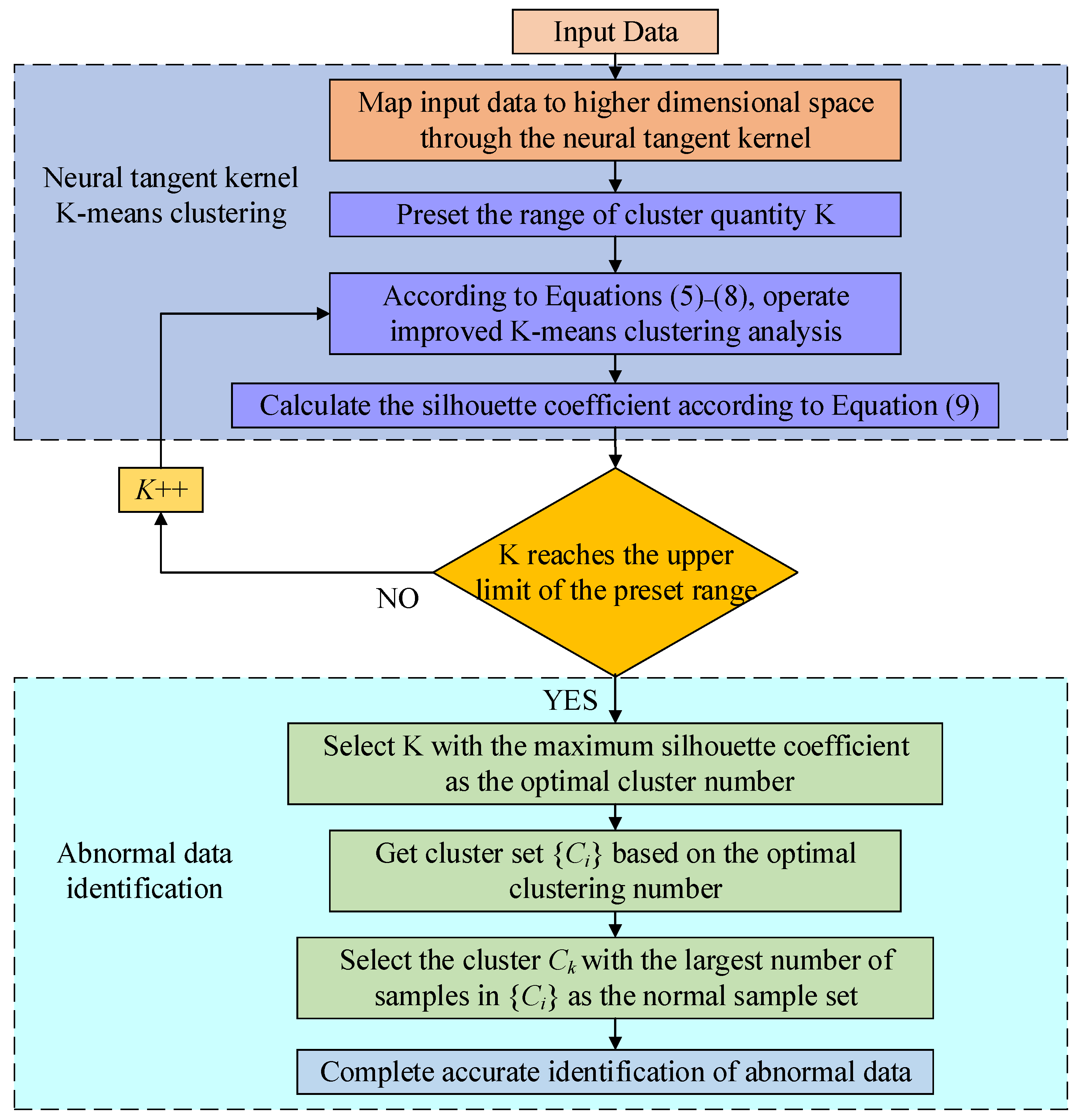
2. Intelligent Identification of Outliers from Single-Source Data based on Neural Tangent Kernels K-Means Clustering

2.1. A Brief Introduction of Kernel K-Means Clustering

Clustering algorithm is a typical unsupervised machine learning method. It uses the characteristics of samples to compare the similarity of samples and divides them with similar attributes into the same class or cluster [12,13]. In order to extract valuable information from complex and diverse data, the kernel method was introduced into the clustering algorithm and kernel clustering algorithm was proposed. Similar to the Support Vector Machine (SVM), the basic idea of kernel clustering is to map the samples of the input space to the high-dimensional feature space with Mercer kernel [14] in order to obtain a more ideal clustering effect in the high-dimensional feature space. Compared with the traditional K-means clustering algorithm, the kernel K-means clustering algorithm has a certain degree of improvement in clustering accuracy, stability and robustness [15,16].

Suppose N M-dimensional samples form the input space $\mathit{X}={\left\{{\mathit{x}}_i\right\}}_{i=1}^n$, ${\mathit{x}}_i\in {\mathit{R}}^{m\times 1}$, the sample needs to be divided into K cluster classes. The kernel K-means clustering method first maps the input dataset to the high-dimensional feature space F through a specific nonlinear mapping function $\phi$, get $\phi (X)={\{\phi (x_i)\}}_{i=1}^n$, then K-means clustering is carried out in high-dimensional space. The clustering center is updated according to the following formula:

$$\phi (c_i)=\frac{1}{n}{\displaystyle \sum _{j=1}^{n_i}{x}_j}; i=1,2,\cdots ,K$$

(1)

where $n_i$ is the number of samples of the i-th clusters. The objective function of kernel K-means clustering is as follows:

$$D=\underset{c_i}{\arg \min }{\displaystyle \sum _{i=1}^k{\displaystyle \sum _{x_j\in c_i}{\Vert \phi (x_j)-\phi (c_i)\Vert }^2}}$$

(2)

where ${\Vert \phi (x_j)-\phi (c_i)\Vert }^2$ is the square of the Euclidean distance from the j-th sample $\phi (x_j)$ to the i-th cluster center $\phi (c_i)$ in the high-dimensional feature space, which is defined as the metric function of the kernel K-means clustering algorithm, as shown in the following formula:

$$d(x_j,c_i)\triangleq {\Vert \phi (x_j)-\phi (c_i)\Vert }^2$$

(3)

Therefore, by finding the minimum value of $d(x_j,c_i)$ and determining which cluster the data point belongs to, the kernel k-means clustering can be completed.

2.2. Neural Tangent Kernel K-Means Clustering Algorithm

2.2.1. Neural Tangent Kernel

Based on the kernel K-means algorithm, the neural tangent kernel K-means clustering algorithm introduces the neural tangent kernel function to complete the nonlinear mapping function. The neural tangent kernel [17,18] originates from the training process of infinite wide deep neural networks. For a neural network which is trained by the gradient descent method, an infinite width deep neural network with proper random initialization, infinitesimal gradient descent step (i.e., gradient flow) is equivalent to a deterministic kernel regression predictor with neural tangent kernel. The neural tangent kernel function can be expressed as:

$$K^{NTK}(\mathit{x},{\mathit{x}}^{\prime })=\langle \frac{\partial f(\theta ,\mathit{x})}{\partial \theta },\frac{\partial f(\theta ,{\mathit{x}}^{\prime })}{\partial \theta }\rangle$$

(4)

where $x,x^{\prime }$ is input data, $f(\theta ,x,x^{\prime })$ is a fully connected neural network and $\theta$ is the set of parameters in the neural network. After high-dimensional mapping of the original data set $\mathit{X}={\left\{{\mathit{x}}_i\right\}}_{i=1}^n$ through the neural tangent kernel function $K^{NTK}$, the kernel matrix $X\_NTK={\{x\_nt{k}_i\}}_{i=1}^n$ is obtained, where cluster analysis is carried out.

2.2.2. Decision of Initial Cluster Centers

The classical K-means clustering algorithm selects the initial clustering center randomly, which has slow convergence speed and poor stability. In order to improve the performance of the algorithm, we consider randomly selecting a data point from the dataset as the center of initial clustering $c_1$, and then calculate the distance $R(x_i)$ between each sample point $x_i$ and the existing cluster center. After that, we calculate the probability of each sample being selected as the next cluster center. The calculation formula is as follows:

$$Q(x_i)=\frac{R(x_i)}{{\displaystyle \sum _{x_i\in X}R(x_i)}}$$

(5)

Then, the next cluster center was selected by the roulette wheel selection method, and K cluster centers were selected by repeating this step.

2.2.3. Update Method of Cluster Centers

The classical K-means clustering algorithm updates the cluster center by calculating the average value of distance between all samples and cluster centers in each cluster. This method has a large amount of computation and low efficiency. In order to improve the performance of the algorithm, an update method of cluster centers which gives consideration to both a small amount of calculation and distance inside or outside the cluster is proposed. In each cluster, take each sample point $x_i$ as the clustering center, respectively, and calculate minimum distance $w_1(x_i)$ of every other sample points within the cluster to the cluster center, and calculate maximum distance $w_2(x_i)$ of the cluster center to every other cluster center, and find the minimum value of the reciprocal sum of $w_1(x_i)$ and $w_2(x_i)$. Therefore, the function of updating the cluster center is as follows:

$$c_i=w_{\min }(x_i)=w_1(x_i)+\raisebox{1ex}{$1$}\!\left/ \!\raisebox{-1ex}{$w_2(x_i)$}\right.$$

(6)

where $w_{\min }(x_i)$ is the basis for the NTKKM clustering algorithm to update the cluster center. When the last cluster center is the same as the current cluster center, which means the cluster center does not change any more, the algorithm iteration ends. In this way, each cluster center can not only represent the sample points of the cluster, but also be as far away from the sample points that do not belong to the cluster as possible.

2.2.4. Objective Function of Clustering Algorithm

Substituting the neural tangent kernel function $K^{NTK}$ of Equation (4) into Equation (2), the objective function of NTKKM is obtained as follows:

$$D_{NTK}(X,C)=\underset{c_i}{\arg \max }{\displaystyle \sum _{i=1}^k{\displaystyle \sum _{x_j\in c_i}{\Vert K^{NTK}(x_j)-K^{NTK}(c_i)\Vert }^2}}$$

(7)

where ${\Vert K^{NTK}(x_j)-K^{NTK}(c_i)\Vert }^2$ is the square of the Euclidean distance of high-dimensional space, which extended from the original input space dependent on the neural tangent kernel, which is now expressed as the metric function of the NTKKM clustering algorithm:

$$d_{NTK}(x_j,c_i)\triangleq {\Vert K^{NTK}(x_j)-K^{NTK}(c_i)\Vert }^2$$

(8)

which cluster the data points that belong and can be judged by calculating the minimum value of $d_{NTK}(x_j,c_i)$.

2.2.5. Determination of Optimal Cluster Number

The neural tangent kernel k-means clustering algorithm is improved in the selection and updating process of the cluster center, but it still has the problem that the optimal number of clusters cannot be determined, as the traditional K-means clustering method do. Therefore, the silhouette coefficient is considered to be introduced on the basis of the neural tangent kernel K-means clustering to help it determine the optimal number of clusters. Silhouette coefficient is a commonly used evaluation index for clustering results. For any cluster, $C_i$, the silhouette coefficient of a single sample, can be calculated by:

$$s=\frac{b-a}{\max (a,b)}$$

(9)

where:

$$a=\frac{1}{n}{\displaystyle \sum _{x_j\in C_i}{(x_j-c_i)}^2}$$

(10)

$$b=\frac{1}{m}{\displaystyle \sum _{x_j\in C_i}{\displaystyle \sum _{x_k\in C_l}{(x_i-x_k)}^2}}$$

(11)

where s is the silhouette coefficient of a single sample; a is the average distance between samples and other samples in the cluster $C_i$; b is the average distance between the sample in cluster $C_i$ and all samples in cluster $C_l$, which is closest to cluster $C_i$; $c_i$ is the center of class $C_i$; m and n represent the number of samples in $C_i$ and $C_l$, respectively.

After the optimal clustering number was determined, the data set was analyzed by neural tangent K-means clustering. The cluster with the largest number of samples is selected as the normal data set, and the rest of the samples are classified as outliers so as to achieve the intelligent identification of outliers. Finally, the identified outliers are directly deleted and filled as missing data afterwards. Figure 1 shows the schematic diagram of the intelligent identification process of outliers based on the neural tangent kernel K-means clustering, and the specific steps are as follows:

Step 1: High-dimensional mapping of the original data set $\mathit{X}={\left\{{\mathit{x}}_i\right\}}_{i=1}^n$ through the neural tangent kernel function $K^{NTK}$ to obtain the kernel matrix $X\_NTK={\{x\_nt{k}_i\}}_{i=1}^n$.

Step 2: Based on the strategy proposed in Section 2.2.2, K initial clustering centers were selected, and the initial clustering results were calculated according to Formula (8).

Step 3: Based on the strategy proposed in Section 2.2.3, the clustering center was updated iteratively until convergence, and the final clustering result was obtained.

Step 4: According to Equations (9)–(11), calculate the silhouette coefficients of different K values, select the K value with the largest silhouette coefficient as the optimal cluster number and output its clustering results.

Step 5: Select the cluster with the largest number of samples as the normal data set, and the rest of the samples are classified as outliers to achieve the intelligent identification of outliers.

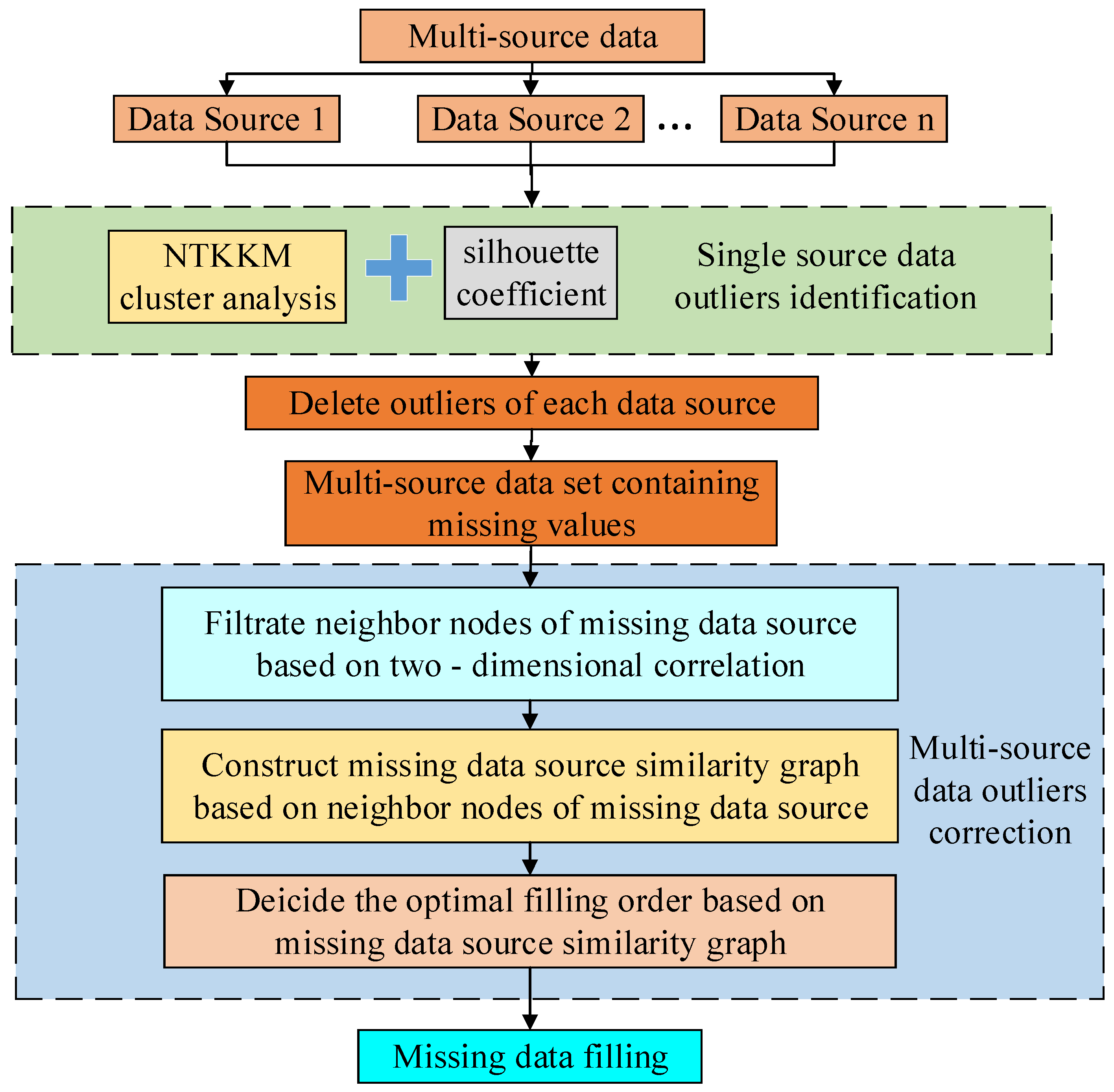
3. Order-Sensitive Correction Strategies of Outlier from Multi-Source Data

In practical engineering, sensory data comes from multi-sources. After the identification of outliers is completed, multiple sensory sources may appear abnormal at the same time, and the distribution of outliers may be relatively dense. After deleting outliers, the problem of correcting original outliers is transformed into the problem of filling multiple densely distributed missing data. In this case, the filling accuracy of the traditional missing data filling method is difficult to guarantee. Therefore, an order-sensitive missing value filling method of multi-source data is proposed to alleviate the problem of filling precision decrease due to the low similarity of the complete neighbor of missing data source in the situation of densely distributed missing data.

3.1. Filtering Neighbor of Missing Data Source Based on Bi-Dimensional Correlation

Suppose that N data sources $S=\{S_1,S_2,\cdots ,S_N\}$ constitute a sensory network. The sensory data set of N data sources at time T is $X^T=\{X_1^T,X_2^T,\cdots ,X_N^T\}$, where each sensory data contains m-dimensional attributes, and the sensory data of data source S_i at time T is $X_i^T=(x_{i1}^T,x_{i2}^T,\cdots ,x_{im}^T)$. Considering the bi-dimensional correlation of different data sources in terms of time and attributes, gray relational degree is used to measure the bi-dimensional similarity between data sources. Assume that there is data missing in the j-th dimension attribute at the current moment, and then the bi-dimensional similarity between data sources S_i and S_k is:

$$Si{m}_{ik}=\frac{1}{1+\min \{d_{ik}^T,d_{ik}^A\}}$$

(12)

where $d_{ik}^T,d_{ik}^A$ represent the similarity of data sources S_i and S_k in time and dimensions attributes, respectively. Assume that the time neighborhood of data $x_{ij}^T$ to be filled in the data source S_i at time T is the data at the t time points forward, i.e., $D_i^T=(x_{ij}^{T-t},x_{ij}^{T-(t-1)},\cdots ,x_{ij}^{T-1})$, and the neighborhood attribute is the data attribute that is correlated with data to be filled $x_{im}^T$, i.e., $D_i^A=(x_{i1}^t,x_{i2}^t,\cdots ,x_{im}^t)$. Corresponding to the time and neighborhood attribute in data source S_k are $D_k^T=(x_{kj}^{T-t},x_{kj}^{T-(t-1)},\cdots ,x_{kj}^{T-1})$ and $D_k^A=(x_{k1}^t,x_{k2}^t,\cdots ,x_{km}^t)$, respectively, then:

$$d_{ik}^T=\frac{1}{t}{\displaystyle \sum _{s=1}^t\frac{\underset{j}{\min } \underset{s}{\min }\left|x_{ij}^{T-(t-s)}-x_{kj}^{T-(t-s)}\right|+\rho \underset{j}{\max } \underset{s}{\max }\left|x_{ij}^{T-(t-s)}-x_{kj}^{T-(t-s)}\right|}{\left|x_{ij}^{T-(t-s)}-x_{kj}^{T-(t-s)}\right|+\rho \underset{j}{\max } \underset{s}{\max }\left|x_{ij}^{T-(t-s)}-x_{kj}^{T-(t-s)}\right|}}$$

(13)

$$d_{ik}^A=\frac{1}{m}{\displaystyle \sum _{s=1}^m\frac{\underset{j}{\min } \underset{s}{\min }\left|x_{is}^t-x_{js}^t\right|+\rho \underset{j}{\max } \underset{s}{\max }\left|x_{is}^t-x_{js}^t\right|}{\left|x_{is}^t-x_{js}^t\right|+\rho \underset{j}{\max } \underset{s}{\max }\left|x_{is}^t-x_{js}^t\right|}}$$

(14)

where $\rho \in (0,1)$ is the adjustment parameter. Based on the above method, the bi-dimensional similarity between each missing data source and the remaining data source can be obtained. The neighboring nodes of the missing data source will be used in the determination of the filling order and the filling process of missing values, and nodes with low similarity have little influence on the determination of the filling order and the filling value. In order to reduce the calculation amount of the construction of the similarity map of the missing data source, the artificial bi-dimensional similarity threshold $\delta$ is used as the similarity screening standard and nodes less than the given threshold are deleted. Then, the nearest neighbor nodes of each missing data source are screened out.

3.2. Decision of Optimal Filling Order and Data Filling Based on Missing Data Source Similarity Graph

In the case of the dense distribution of missing data, data missing may also occur in the near neighbor nodes of missing data sources. At this time, using the existing missing data filling method will lead to lower accuracy of the filling value, or even fail to fill the missing value. In this paper, the filled missing values are used as observations for the subsequent filling process. However, the accuracy of the filled missing values will directly affect the accuracy of the subsequent filling values. Therefore, how to determine an optimal filling order to improve the accuracy of the filling values becomes a challenging and urgent problem. In this paper, the set of missing data sources is constructed as a similarity graph structure, and then, based on the similarity graph, the filling order decision problem is transformed into an optimization problem and solved.

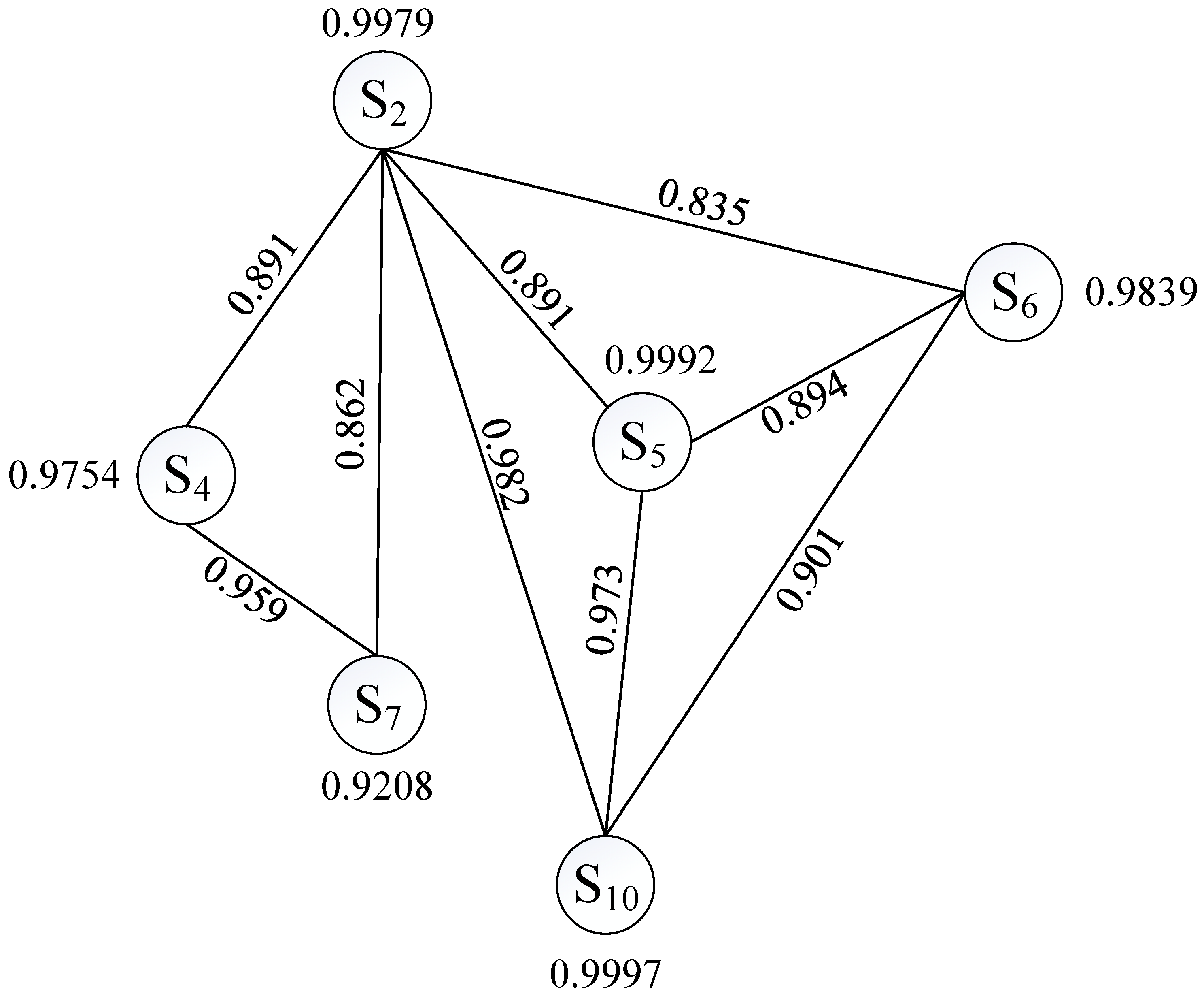
3.2.1. Construction of MISSING data Source Similarity Graph Based on Similarity Analysis

Based on the similarity between missing data source and each neighbor node, a similarity graph centered on missing data source is constructed. Since the construction of similarity graph is mainly used to determine the filling order of missing data source, the vertex of the graph is the missing data source, and the vertex weight is the result of fusion similarity between the missing data source and all its relatively complete neighbors. The edge of the graph represents that two missing data sources are neighbor to each other, and the edge weight is the similarity of the two data sources. Thus, an undirected weighted similarity graph that can directly reflect the dependence between missing data sources is constructed. The similarity between two missing data sources is reflected by the edge weight, and the distribution of all relatively complete neighbor nodes of each missing data source is reflected by the vertex weight. The calculation formula of vertex weight is as follows:

$$w_{s_i}=1-{\displaystyle \prod _{s_k\in N(s_i)}(1-Si{m}_{ik})}$$

(15)

where $N(S_i)$ is the relatively complete set of neighbor nodes of data source $S_i$, and $Si{m}_{ik}$ is the bi-dimensional similarity of data source $S_i$ and $S_k$.

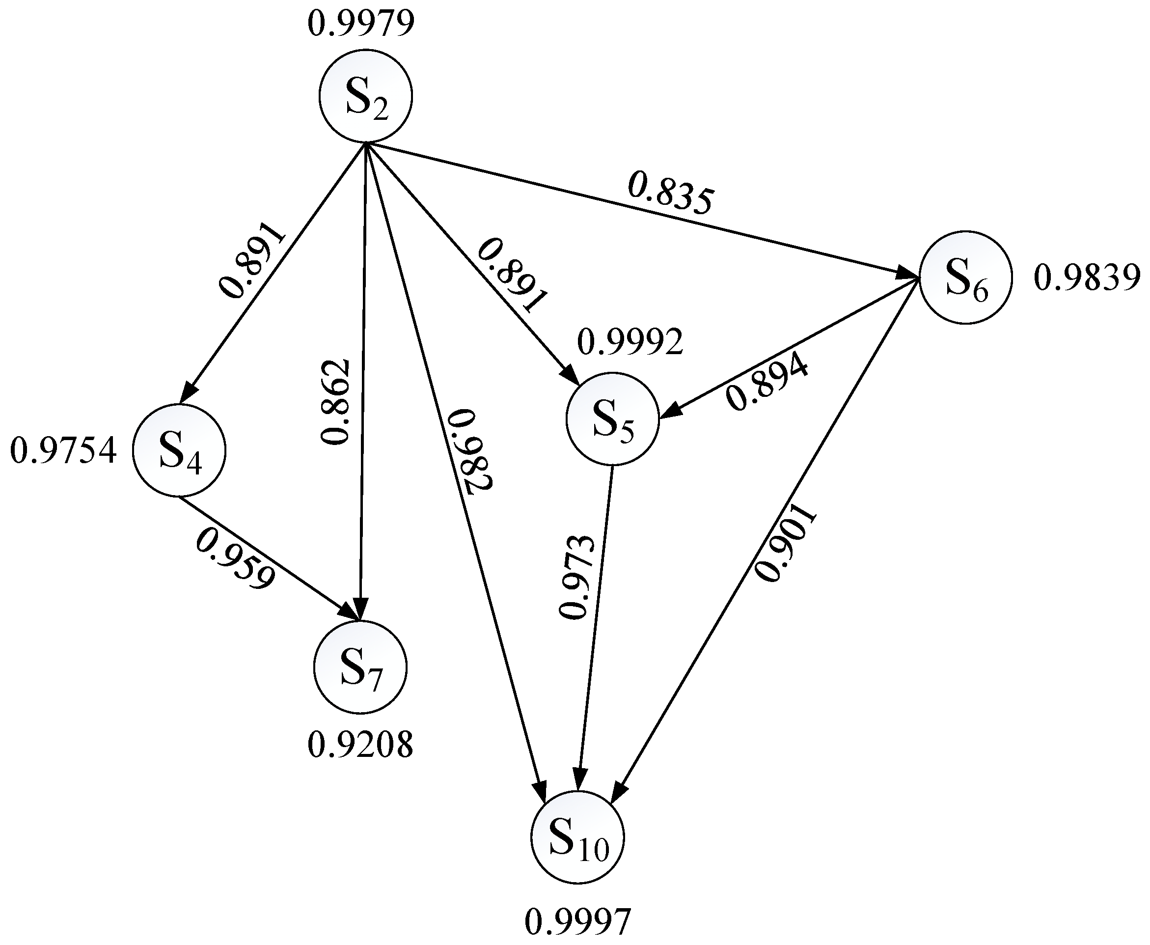
3.2.2. Decision of Optimal Filling Order Based on Missing Data Source Similarity Graph

Further analysis based on the similarity graph of missing data sources in Section 3.2.1 shows that: when a filling order is given, the filling priority of each pair of missing data sources that are neighbors to each other (i.e., connected by an edge) can be determined, and then the corresponding undirected weighted similarity graph can be transformed into a directed weighted similarity graph. For a possible filling order $seq$ containing n missing data sources, the corresponding directed weighted similarity graph is regarded as a Bayesian network. The vertex weight is the prior probability of each vertex in the Bayesian network, the edge weight is the conditional probability between two vertices, and the joint probability of the Bayesian network is the confidence of the corresponding filling order. The formula of joint probability is as follows:

$$b(seq)={\displaystyle \prod _{i=1}^{n}p(S_i|S_{N(i)})}$$

(16)

where $S_{N(i)}$ is the set of missing neighbor nodes that can be used in the filling progress of missing data source $S_i$. When a missing data source is filled, it can be regarded as the observed value and used in the subsequent missing value filling process. Therefore, after the filling order is determined, the neighbor nodes of the missing data source after filling are dynamically changed, and the vertex weights are also dynamically updated. $p(S_i|S_{N(i)})$ is the updated vertex weight value of vertex $S_i$ after $S_{N(i)}$ is added to the list of neighbor nodes that can be used in the filling progress, and its calculation formula is as follows:

$$p(S_i|S_{N(i)})=\{\begin{array}{l}{w}_{s_i}, S_{N(i)}=\varnothing \\ 1-(1-w_{s_i}){\displaystyle \prod _{S_j\in S_{{}_{N(i)}}}(1-Si{m}_{ij})}, S_{N(i)}\ne \varnothing \end{array}$$

(17)

For missing data source $S_i$, the larger $p(S_i|S_{N(i)})$ is, the smaller the filling error is. For a given filling order, the higher the confidence is, the smaller the filling error is. Therefore, the optimal filling sequential decision problem can be transformed into a Bayesian network problem with the highest confidence. Suppose that the set of all possible filling orders of n missing data sources is $SEQ=\{se{q}_1,se{q}_2,se{q}_3,\cdots \}$, and the confidence coefficient of filling order $se{q}_i$ is $b(se{q}_i)$, then the filling order decision problem is transformed into the sequence with the highest confidence coefficient:

$$se{q}^{*}=\arg \max (b(se{q}_i)), se{q}_i\in SEQ$$

(18)

By enumerating all possible filling sequences, the sequence with the highest confidence is selected as the optimal filling sequence, and the optimal solution is obtained. When the sequence of missing data source filling is determined, missing data can be filled in turn.

3.2.3. Data Filling Method Based on Missing Data Source Similarity Graph

In the traditional KNN filling method, K nearest neighbor nodes should be selected for each missing data source to fill the missing value. However, due to the uneven distribution of the nearest neighbor nodes of each missing data source, it is difficult to determine the value of K: if the K value is too small, the filling result will be sensitive to noise and the filling accuracy will decrease. If K value is too large, the nearest neighbor node set will contain a large number of nodes with low similarity to the point to be filled, which will also reduce the filling accuracy and increase the amount of calculation. Therefore, we improved the KNN filling algorithm and proposed a new neighbor-based imputation method (NI). For data source $S_i$ to be filled, set its neighbor node set as $N{S}_i=\{S_1,S_2,\cdots ,S_{\left|N{S}_i\right|}\}$, then the filling value ${\widehat{d}}_i$ of $S_i$ can be calculated by the following formula:

$${\widehat{d}}_i=\frac{{\displaystyle \sum _{S_j\in N{S}_i}Si{m}_{ij}\cdot d_j}}{{\displaystyle \sum _{S_j\in N{S}_i}Si{m}_{ij}}}$$

(19)

This method does not limit the size of the K value, but based on the constructed similarity graph of missing data source, all neighboring nodes whose similarity with the data source to be filled is higher than the given threshold is used to fill. Its advantage is that for each data to be filled, the distribution of its nearest neighbor nodes is considered to find the nearest neighbor nodes suitable for filling, instead of finding fixed K nearest neighbor nodes for all data sources to be filled. Different from the existing KNN or regression filling algorithms, the NI filling algorithm searches for the missing data source’s neighbor based on the bi-dimensional similarity of sensory data, rather than a one-dimensional similarity. Therefore, the nearest neighbor nodes used for missing data source filling are more comprehensive and can further improve the accuracy of filling values. The progress of identification and order-sensitive correction of outliers from multi-sources based on historical data mining is shown in Figure 2, and the specific steps are as follows:

Step 1: Based on the strategy proposed in Section 2.2, operate the neural tangent k-means clustering analysis on the historical data of each data source to identify and delete abnormal data.

Step 2: Based on the strategy proposed in Section 3.1, calculate the bi-dimensional similarity between data sources and screen the missing data source neighbor nodes.

Step 3: Based on the strategy proposed in Section 3.2.1 and the screening results of the nearest neighbor nodes of the missing data source, construct the similarity graph centered on the missing data source.

Step 4: Based on the strategy proposed in Section 3.2.2, the optimal filling sequential decision making problem was transformed into a Bayesian network problem with the highest confidence coefficient selected for solving, so as to realize the optimal filling sequential decision making.

Step 5: Based on the strategy proposed in Section 3.2.3 and the optimal filling sequence, fill the missing data according to Equation (19) to realize abnormal data correction.

4. Case Experiment and Analysis

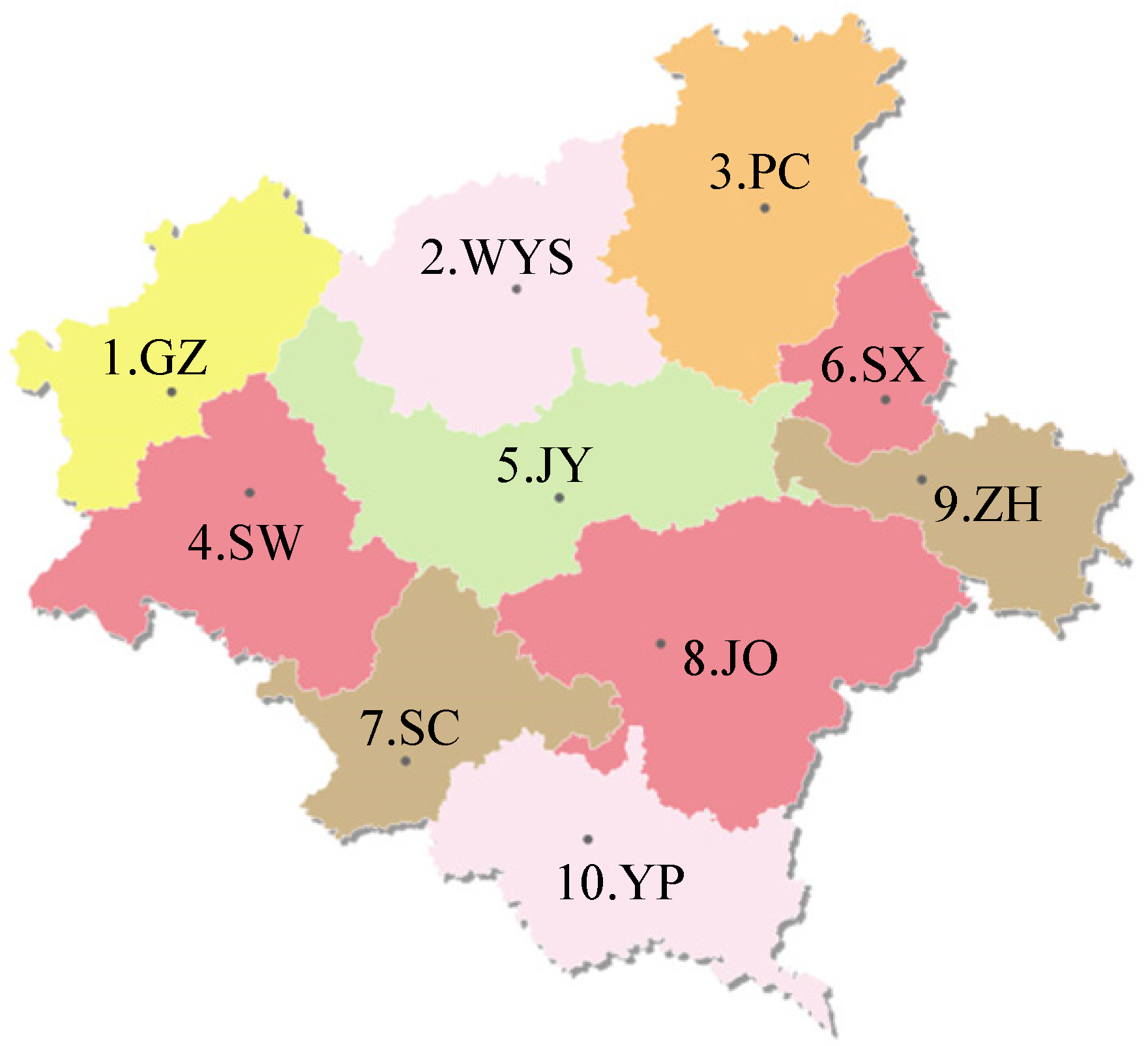
4.1. Case Background Introduction

To verify the validity and rationality of the method proposed in this paper, taking the actual line loss rate data of a regional power grid in a city of China as the experimental object. The region contained 10 data sources including GZ, WYS, PC, SX, JY, SW, ZH, JO, SC and YP, numbered from 1 to 10, respectively. The distribution of data sources is shown in Figure 3. The data sampling interval is one day, and the monitoring value includes line loss rate, power consumption, electricity input of superior grid, input and output power of same level grid, electricity input of different power supply types, electricity input of distributed power supply, etc. The computer is configured as AMD 3500× with 16 GB memory and Python3.6 programming language. The initialization of neural tangent kernel function is performed by NEURAL TANGENTS apps developed by Google. The network structure consists of three layers, the input layer contains 1 neuron, the hidden layer contains 64 neurons, and the output layer contains 16 neurons. The active function between each layer is RELU.

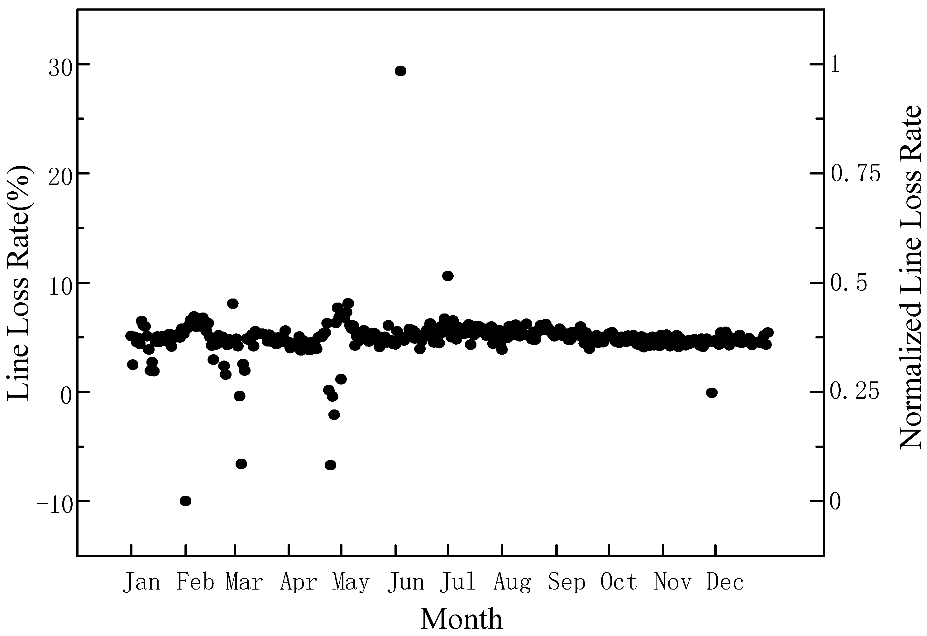
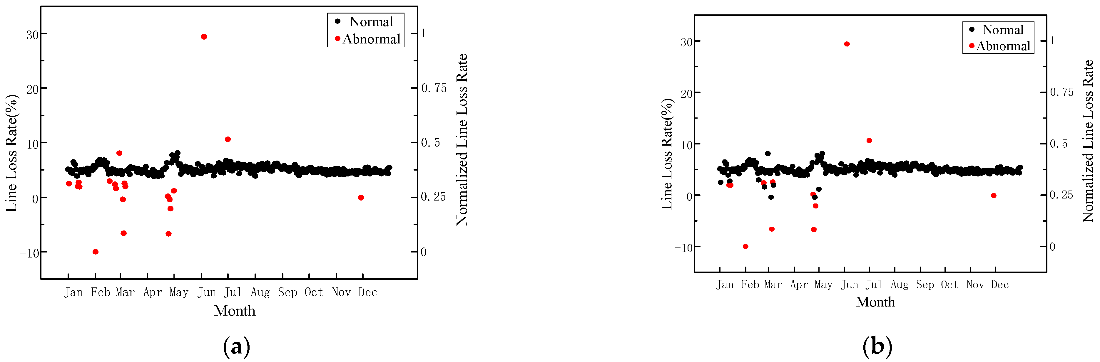
4.2. Outliers Identification Analysis of Single-Source Data Based on Neural Tangent Kernel K-Means Clustering

Firstly, taking data source YP as an example, the historical line loss rate data is normalized. The actual value and normalized value distribution of YP historical line loss rate are shown in Figure 4. It can be seen from the figure that line loss is mainly distributed within the interval [0, 10], but there are several isolated points. If directly using the NTKKM clustering algorithm for analysis, the cluster number needs to be set manually, which is highly subjective, leading to difficulty in determining the optimal cluster number of the sample set. Therefore, the silhouette coefficient is considered to determine the optimal cluster number of the sample set.

Table 1. Clustering performance comparison of different clustering algorithms.

K	NTKKM	K-Means
2	0.441	0.402
3	0.502	0.395
4	0.425	0.432
5	0.404	0.312
6	0.371	0.291

shows the calculation results of the silhouette coefficient of NTKKM and traditional K-Means clustering in different clustering number. It can be seen that when K is 3, the silhouette coefficient reaches the maximum value. Therefore, the optimal cluster number is set as 3.

Cluster analysis of line loss samples was carried out based on the optimal cluster number, and the clustering results are shown in Figure 5. As can be seen from Figure 5, the samples marked with black have the largest quantity, which is the main body of the cluster. Therefore, they are discriminated as normal value, and the rest are outliers. Figure 5b presents the clustering results of traditional K-means clustering. It can be seen from the comparison of Figure 5a,b, in the case of maximum silhouette coefficients, the NTKKM clustering algorithm can identify abnormal line loss data more accurately. Compared with the traditional clustering algorithm, the NTKKM clustering algorithm can effectively identify samples with abnormally low loss values in the interval [0, 3].

Through the above methods, the historical data of the line loss rate of each data source in the regional power grid are clustered separately. Delete abnormal data and enter the following missing data filling progress.

4.3. Missing Data Source Neighbor Node Filtering and Similarity Graph Construction Analysis

Table 2. Missing data of multi-source line loss rate after deletion operation.

Date	GZ	WYS	PC	SW	JY	SX	…
24 July	√	×	√	×	×	×	…
2 July	×	√	×	√	√	×	…
3 June	√	√	×	√	√	√	…
9 December	×	×	√	√	√	√	…
3 March	√	√	×	×	×	×	…
13 May	√	×	√	√	×	√	…
…	…	…	…	…	…	…	…

shows part of the data missing of the multi-source line loss rate after the deletion operation. As can be seen, there were many cases of the dense distribution of missing data. At this time, the nodes adjacent to the missing data source also have data missing. The existing data filling method is hard to operate, even failing to fill missing data. Therefore, an order-sensitive multi-source data missing value filling framework is considered to fill missing data.

Taking the data loss of multi-source line loss rate on July 24 as an example, there were 6 data sources missing on that day, namely WYS, SW, JY, SX, SC and YP (No. 2, No. 4, No. 5, No. 6, No. 7 and No. 10). Firstly, the bi-dimension similarity analysis method in Section 3.1 is used to calculate and screen the similarity of the nearest neighbor nodes of each missing data source, and the results are shown in

Table 3. Calculation results of the two dimensional similarity between missing data sources and remaining data sources.

Data Source Number	1	2	3	4	5	6	7	8	9	10
2	0.897	—	0.894	0.891	0.92	0.835	0.862	0.889	0.881	0.982
4	0.995	0.891	0.992	—	0.755	0.694	0.959	0.977	0.800	0.541
5	0.761	0.92	0.759	0.755	—	0.894	0.735	0.757	0.977	0.973
6	0.794	0.835	0.697	0.694	0.894	—	0.698	0.696	0.838	0.901
7	0.953	0.862	0.956	0.959	0.735	0.698	—	0.958	0.698	0.727
10	0.973	0.982	0.889	0.541	0.973	0.901	0.727	0.803	0.749	—

.

Set the threshold of bi-dimension similarity $\delta =0.8$; the list of nearest neighbor nodes of each missing data source is shown in

Table 4. List of neighbor nodes of each missing data source.

Data Source Number	Neighboring Data Sources
2	1, 3, 4, 5, 6, 7, 8, 9, 10
4	1, 2, 3, 7, 8, 9
5	2, 6, 9, 10
6	2, 5, 9, 10
7	1, 2, 3, 4, 8
10	1, 2, 3, 5, 6, 8

. Based on the list of neighbor nodes of the missing data source, the similarity graph of the missing data source can be drawn, as shown in Figure 6.

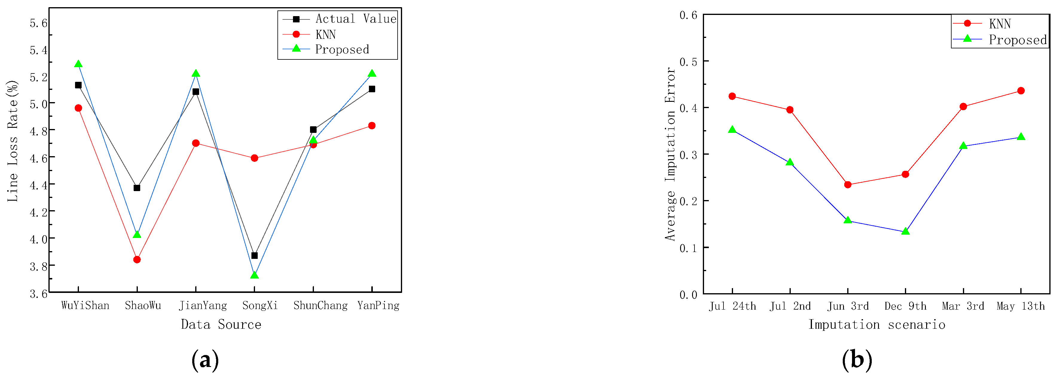
4.4. Optimal Filling Order Decision and Filling Effect Analysis

Based on the constructed missing data source similarity graph, if a filling order is given, the filling priority of two missing data sources can be determined for each pair of mutually adjacent nodes (i.e., connected by an edge). Then, the corresponding undirected weighted similarity graph can be transformed into a directed weighted similarity graph. Taking the filling sequence (2, 4, 6, 5, 10, and 7) as an example, the directed weighted similarity diagram is drawn as shown in Figure 7, the arrows between data sources in the figure point from the data source filled first to the data source filled later.

Based on the similarity graph of directed missing data source, the confidence and average filling error of all filling orders are calculated by Equation (16), as shown in

Table 5. Part of filling order and its confidence.

Imputation Order Sequence	Confidence	Average Filling Error
(2, 4, 5, 6, 7, 10)	0.5875	0.2326
(4, 2, 5, 6, 7, 10)	0.6349	0.1875
(2, 4, 6, 5, 7, 10)	0.6320	0.1898
(2, 4, 7, 5, 6, 10)	0.6001	0.2103
…	…

. Through sorting, the filling sequence with the maximum confidence is finally selected and fills in the original missing data according to Equation (19). The average filling error $avg\_imperr$ is defined as follows: For $n$ missing data sources in a filling scenario, the filling value of the i-th missing data source is set as ${\widehat{d}}_i$ and the actual value is $d_i$, then the calculation formula of the average filling error $avg\_imperr$ is as follows:

$$avg\_imperr=\frac{1}{n}{\displaystyle \sum _{i=1}^n\left|\frac{{\widehat{d}}_i-d_i}{d_i}\right|}$$

(20)

In the scene of 24 July, the filling results of the proposed method and KNN algorithm are compared, as shown in Figure 8a. It can be seen that the filling value of the proposed method is closer to the real value than that of the KNN algorithm. In the partial filling scenario, the average filling error of the proposed method and KNN algorithm is shown in

Table 6. Average filling errors of the proposed method and KNN algorithm in partial filling scenarios.

Imputation Scenario and Amounts of Abnormal Data Source	KNN	Proposed Method
Jul 24th (6)	0.4238	0.3510
Jul 2nd (4)	0.3944	0.2813
Jun 3rd (2)	0.2341	0.1566
Dec 9th (2)	0.2563	0.1329
Mar 3rd (5)	0.4017	0.3163
May 13th (5)	0.4356	0.3358
…	…	…

and Figure 8b. It can be seen that the average filling error of the proposed method is lower than that of the KNN algorithm. In the filling scenario with many missing data sources, the average filling error of the proposed method decreases by approximately 20% compared with the KNN algorithm. This indicates that the method proposed has obvious advantages in the case of a large number of missing data sources and relatively dense data sources. In actual projects, the correction of abnormal line loss rate requires recount and calculation of various data, which often takes several working days. The method proposed in this paper has high correction accuracy and short calculation time, which can provide support for the identification and correction of abnormal data in practical engineering.

5. Conclusions

In this paper, an intelligent identification and order-sensitive correction method of outliers from multi-data sources based on historical data mining was proposed. Firstly, an accurate intelligent identification method of outliers of single-source data is proposed based on the Neural Tangent Kernel K-means (NTKKM) clustering algorithm. Input data space is mapped to high-dimensional feature space through Neural Tangent Kernel. Then, in the high-dimensional feature space, abnormal data features are mined by K-means clustering, which are identified and deleted for subsequent filling operations. Secondly, for the filling problem of multiple densely distributed missing data, an order-sensitive missing value imputation framework for multi-source sensory data (OMSMVI) was proposed. Considering that the filled missing values are used as reference values for subsequent filling, the filling order decision problem is transformed into an optimization problem to decide the optimal filling order of missing values in multi-source data. Finally, aiming at the problem that the K value of the traditional KNN filling algorithm is difficult to determine, a Neighborhood-based Imputation (NI) algorithm is proposed to improve the traditional KNN filling algorithm. Using the multidimensional similarity of multi-source data to find all the neighbors of the missing data source, the nearest neighbor nodes suitable for filling was found, and the missing data can be filled and the abnormal data can be corrected. An example of actual power grid data of a China city is set as the experimental object, we compared the proposed clustering and missing data filling algorithm with the traditional method. The results show that the proposed clustering method can realize the effective partition of abnormal data more accurately compared with the traditional clustering algorithm, and the determined optimal filling sequence has higher accuracy. The proposed method provides a feasible new idea for intelligent identification and correction of abnormal data in the process of data preprocessing.

References

1. Zhang, N. Methodolgical Progress Note: Handling Missing Data in Clinical Research. J. Hosp. Med. 2020, 14, 237–239. [Google Scholar] [CrossRef] [PubMed]
2. Gomila, R.; Clark, C.S. Missing data in experiment-s: Challenges and solutions. Psychol. Methods 2020, 2, 66–71. [Google Scholar] [CrossRef] [PubMed]
3. Wang, R.; Ji, W.; Liu, M.; Wang, X.; Weng, J.; Deng, S.; Gao, S.; Yuan, C. Review on mining data from multiple data sources. Pattern Recognit. Lett. 2018, 109, 120–128. [Google Scholar] [CrossRef]
4. Mahmud, M.S.; Huang, J.Z.; Salloum, S.; Emara, T.Z.; Sadatdiynov, K. A survey of data partitioning and sampling methods to support big data analysis. Big Data Min. Anal. 2020, 3, 85–101. [Google Scholar] [CrossRef]
5. Markovsky, I. A Missing Data Approach to Data-Driven Filtering and Control. IEEE Trans. Autom. Control. 2017, 62, 1972–1978. [Google Scholar] [CrossRef]
6. Chuan, S.; Yueyi, C.; Cheng, C. Imputation of missing data from offshore wind farms using spatio-temporal correlation and feature correlation. Energy 2021, 229, 92–104. [Google Scholar] [CrossRef]
7. Shao, N.; Chen, Y. Abnormal Data Detection and Identification Method of Distribution Internet of Things Monitoring Terminal Based on Spatiotemporal Correlation. Energies 2022, 15, 2151. [Google Scholar] [CrossRef]
8. Ma, Y.; Zhao, X.; Zhang, C.; Zhang, J.; Qin, X. Outlier detection from multiple data sources. Inf. Sci. 2021, 580, 819–837. [Google Scholar] [CrossRef]
9. Chang, X.; Qiu, Y.; Su, S.; Yang, D. Data Cleaning Based on Stacked Denoising Autoencoders and Multi-Sensor Collaborations. Comput. Mater. Contin. 2020, 63, 691–703. [Google Scholar]
10. Kermorvant, C.; Liquet, B.; Litt, G.; Jones, J.B.; Mengersen, K.; Peterson, E.E.; Hyndman, R.J.; Leigh, C. Reconstructing Missing and Anomalous Data Collected from High-Frequency In-Situ Sensors in Fresh Waters. Int. J. Environ. Res. Public Health 2021, 18, 12803. [Google Scholar] [CrossRef] [PubMed]
11. Wang, Z.; Wang, L.; Huang, C. A Fast Abnormal Data Cleaning Algorithm for Performance Evaluation of Wind Turbine. IEEE Trans. Instrum. Meas. 2021, 70, 5006512. [Google Scholar] [CrossRef]
12. Gondeau, A.; Aouabed, Z.; Hijri, M.; Peres-Neto, P.R.; Makarenkov, V. Object Weighting: A New Clustering Approach to Deal with Outliers and Cluster Overlap in Computational Biology. IEEE/ACM Trans. Comput. Biol. Bioinform. 2021, 18, 633–643. [Google Scholar] [CrossRef] [PubMed]
13. Huang, D.; Wang, C.-D.; Peng, H.; Lai, J.; Kwoh, C.-K. Enhanced Ensemble Clustering via Fast Propagation of Cluster-Wise Similarities. IEEE Trans. Syst. Man Cybern. Syst. 2021, 51, 508–520. [Google Scholar] [CrossRef]
14. Zhang, M.; Wang, X.; Chen, X.; Zhang, A. The Kernel Conjugate Gradient Algorithms. IEEE Trans. Signal Process. 2018, 66, 4377–4387. [Google Scholar] [CrossRef]
15. Yao, Y.; Li, Y.; Jiang, B.; Chen, H. Multiple Kernel k-Means Clustering by Selecting Representative Kernels. IEEE Trans. Neural Netw. Learn. Syst. 2021, 32, 4983–4996. [Google Scholar] [CrossRef] [PubMed]
16. Lu, J.; Lu, Y.; Wang, R.; Nie, F.; Li, X. Multiple Kernel K-Means Clustering with Simultaneous Spectral Rotation. In Proceedings of the ICASSP 2022—2022 IEEE International Conference on Acoustics, Speech and Signal Processing (ICASSP) 2022, Singapore, 23–27 May 2022; pp. 4143–4147. [Google Scholar] [CrossRef]
17. Nguyen, T.V.; Wong, R.K.W.; Hegde, C. Benefits of Jointly Training Autoencoders: An Improved Neural Tangent Kernel Analysis. IEEE Trans. Inf. Theory 2021, 67, 4669–4692. [Google Scholar] [CrossRef]
18. Alemohammad, S.; Babaei, H.; Balestriero, R.; Cheung, M.Y.; Humayun, A.I.; LeJeune, D.; Liu, N.; Luzi, L.; Tan, J.; Wang, Z.; et al. Wearing A Mask: Compressed Representations of Variable-Length Sequences Using Recurrent Neural Tangent Kernels. In Proceedings of the ICASSP 2021—2021 IEEE International Conference on Acoustics, Speech and Signal Processing (ICASSP) 2021, Toronto, ON, Canada, 6–11 June 2021; pp. 2950–2954. [Google Scholar]
Figure 1. Schematic diagram of intelligent identification process of outliers based on neural tangent kernel K-means clustering.
Electronics 11 02819 g001
Figure 2. Intelligent identification and order-sensitive correction progress of outliers from multi-source data based on historical data mining.
Electronics 11 02819 g002
Figure 3. Distribution of data sources of regional power grid.
Electronics 11 02819 g003
Figure 4. Distribution of historical line loss rate of data source YP.
Electronics 11 02819 g004
Figure 5. Clustering result of historical line loss rate: (a) NTKKM clustering results. (b) Traditional K-means clustering results.
Electronics 11 02819 g005
Figure 6. Similarity graph of missing data source.
Electronics 11 02819 g006
Figure 7. Similarity diagram of directed missing data source.
Electronics 11 02819 g007
Figure 8. (a) Comparison between the filling results of the proposed method and KNN algorithm and the real value (scene on 24 July). (b) Comparison of average filling errors between the proposed method and KNN algorithm in partial filling scenarios.
Electronics 11 02819 g008