
A Cloud Based Optimization Method for Zero-Day Threats Detection Using Genetic Algorithm and Ensemble Learning

 , , ,
, , ,
Abstract
:1. Introduction
1.1. Research Question
- Is there any classification performance difference in terms of optimization using the UGRansome1819 dataset?
1.2. Aim and Objectives
- Use SVM, NB, and RF classifiers to determine if the classifier’s assumptions are exact. We have examined and trained those classifiers using SageMaker.
- Compare the classifiers in terms of spotting 0-days threats and apply the GA on the UGRansome1819 dataset to extract salient features.
- Use the GA optimizer with each classifier to evaluate the improved performance.
- Use Ensemble Learning to combine the results of classifiers and determine if this method enhances the classification performance.
- Lastly, compare the outcomes and the UGRansome1819 performance and complexity with existing datasets with the same algorithms and optimization settings by computing them on the CAIDA and UNSWNB-15 datasets.
2. Related Works
2.1. Anomaly Intrusion Detection System (AIDS)
2.2. UGRansome1819 Dataset
- The Transmission Control Protocol (TCP) carries the most characteristics in terms of network protocols (92,157).
- The AF flag has the most features (72,814).
- Locky has the most features in terms of ransomware family (33,870).
- Addressing of class 1DA11mPS has the most properties (82,048).
- In comparison to classes B, A, and D, class C of IP addresses has much more characteristics (95,508).
- The Secure Shell (SSH) threat has the most attributes (34,972) compared to UDP Scan, Blacklisted, Spamming, DoS, Scan, and Bonet threats.
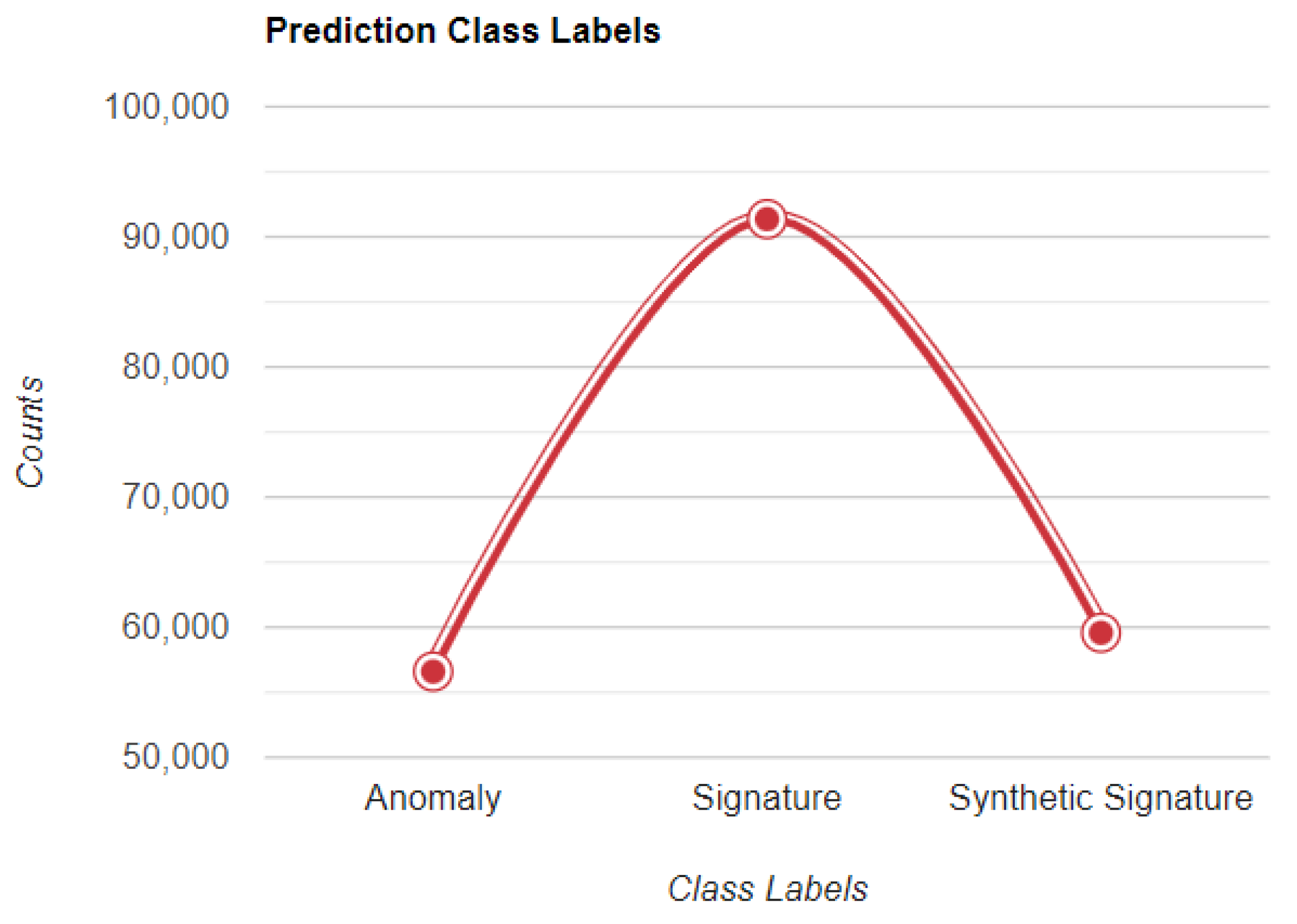
- The Signature (S) threat category has by far the most properties compared to the Synthetic Signature (SS), and Anomaly (A) threats predictions.
- The A category represents unknown threats without signature keys. This prediction includes the most 0-day threats.
- The SS category includes unknown and known threats with and without signature keys. This prediction exhibits both, regularity and irregularity.
- The S category depicts well-known threats with updated signature keys. This prediction portrays regularity or normality.
2.3. Support Vector Machine Algorithm
2.4. Naive Bayes Algorithm
2.5. Random Forest
| Algorithm 1 Random Forest Algorithm |
|
2.6. Ensemble Model Technique
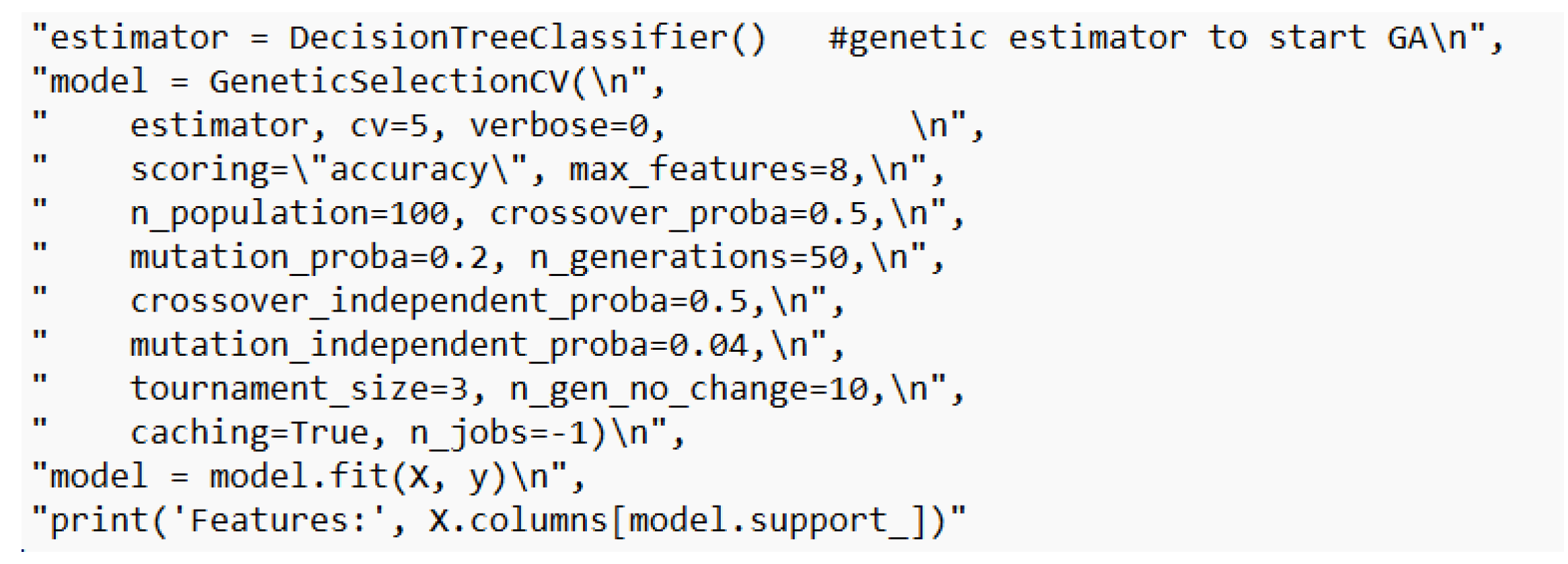
2.7. Genetic Algorithm
- Use the initial dataset (population) to search for a possible solution s. The algorithm starts with a population that can be thought of as a set of individuals. Each individual represents a solution to the optimization problem. The solution is characterized by a set of variables (parameters) called “genes” that are merged into a string to produce a solution (chromosome). We have used ternary values (0, 1, and 2) to represent a set of genes. This can be viewed as encoding genes into a chromosome.
- Calculate the fitness function. It determines how to fit a solution by comparing it to other solutions and providing a fitness score for each solution. The probability that a solution will be selected is based on the fitness score. The probability of selecting a solution is denoted by P[s]. We posit that and are constant:
- Selection. This phase selects the fittest solutions and lets them pass their genes to the next iteration. This is like how it is the fittest individuals that pass their genes to the next generation in Darwinism. The parents of individuals are selected using the fitness scores. To be selected for reproduction, individuals should have high fitness. It utilizes a probability distribution for selection where the given string should have a selection probability proportional to its fitness. The mathematical formulation of the selection process probability (Prob.) is:
- Compute the crossover process. A crossover point is selected for each pair of parents to be mated. This is a random process within genes where offspring are created by merging the parents’ genes among themselves to reach a crossover point and new offspring are included in the population. Crossover replaces some parent’s genes by corresponding them with the genes of other parents. If we have two strings x and y, each having three variables:This represents possible solutions to the classification problem. Two cross-points are randomly selected and a new possible solution is produced by merging the string of the original parents. For example, the offspring solution would be
- Implement the mutation process. Genes of offspring formed are subjected to a mutation using a minimalistic random probability: String’s bits are flipped to maintain the population diversity. The flip mutation selects random bits and flips them differently. The bold indicates the permutation or the bytes that have been changed or flipped during the process:When the population convergence is achieved, the GA terminates and provides a set of solutions to the optimization problem.
2.8. Summary of Related Works
3. Materials and Methods
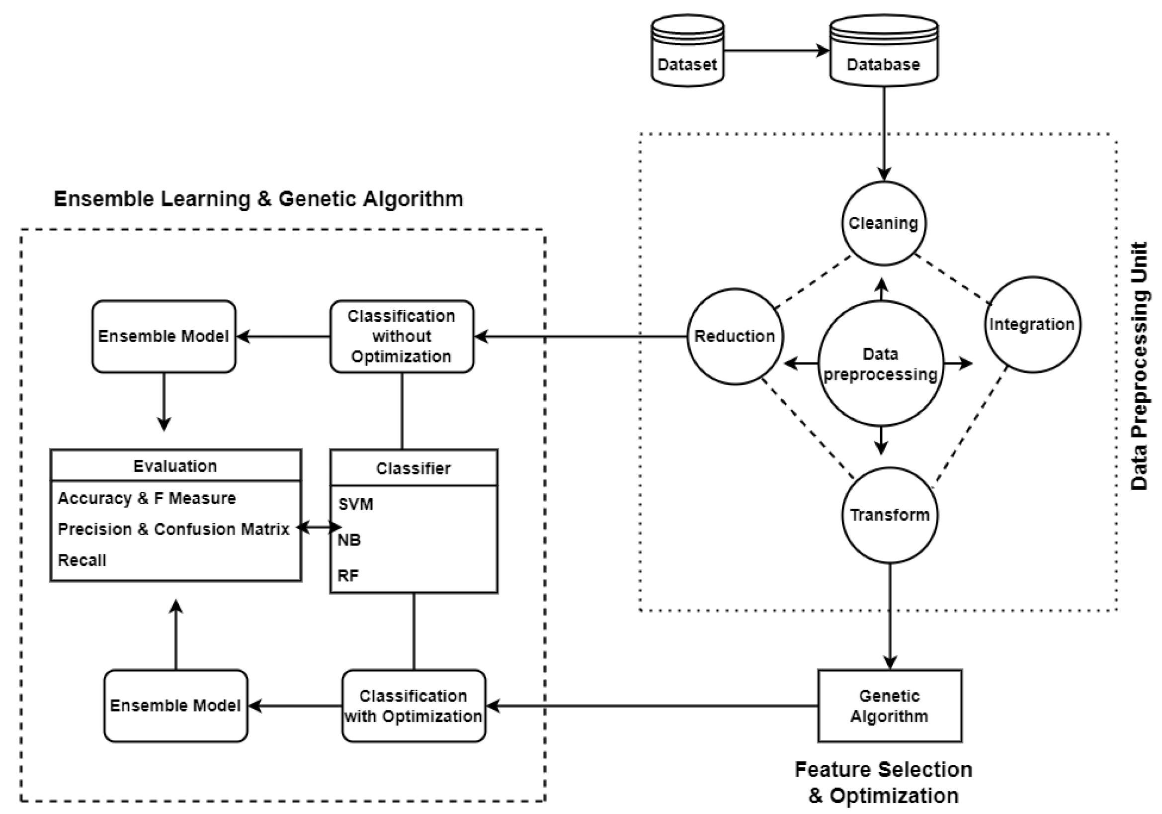
3.1. The Proposed Model
3.2. Data Pre-Processing
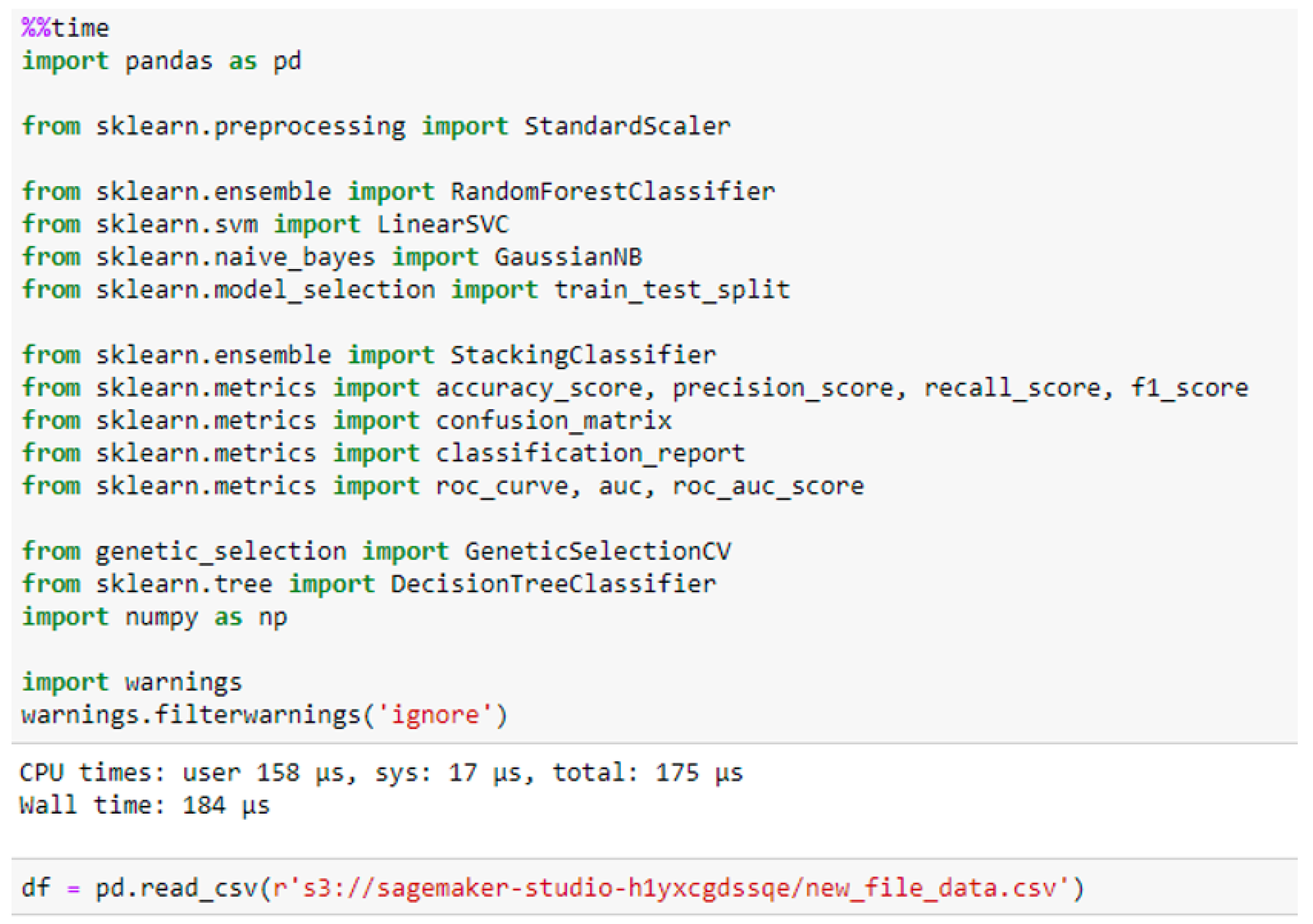
3.3. Specifications of Software and Hardware
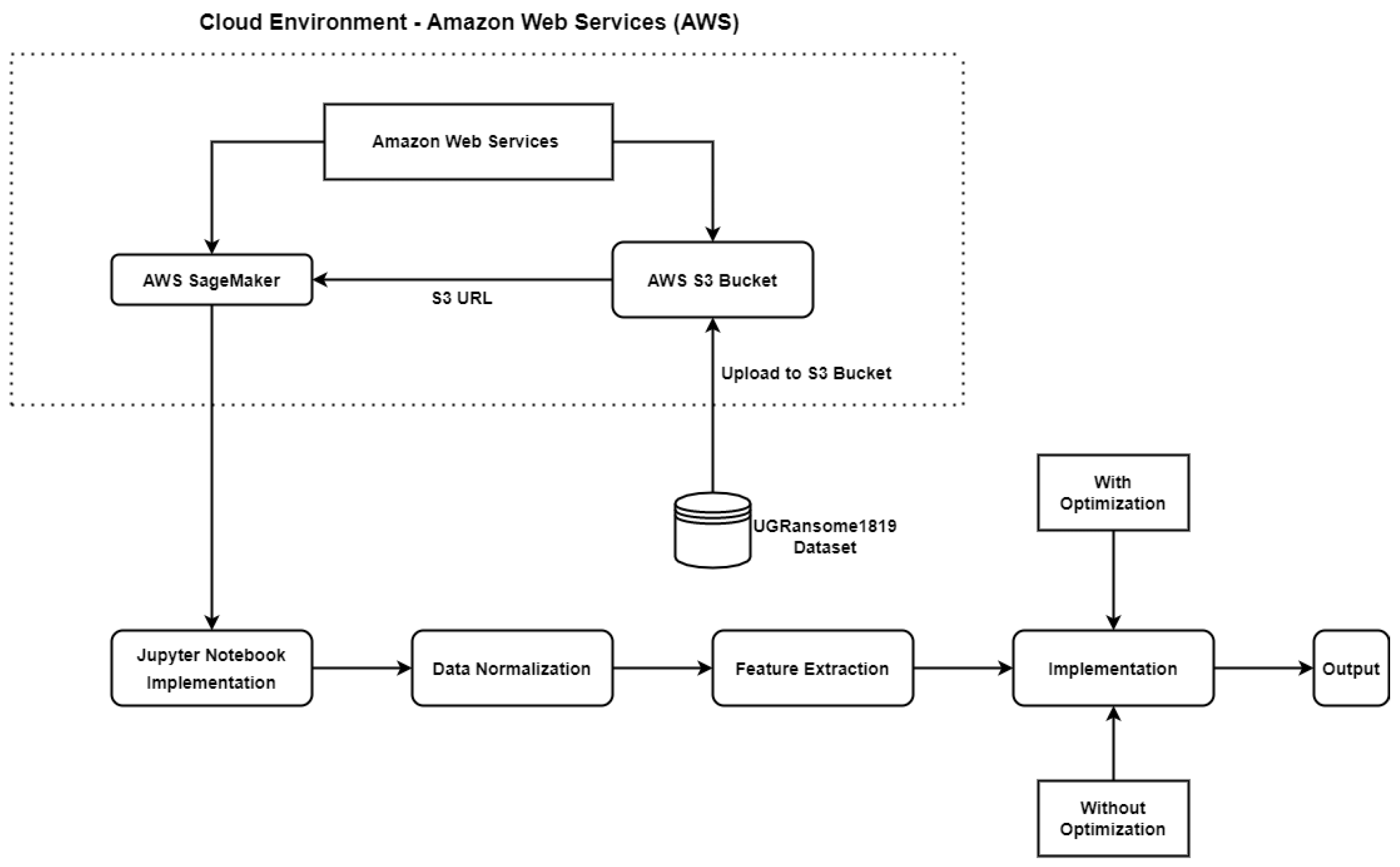
3.4. Cloud Services
4. Implementation
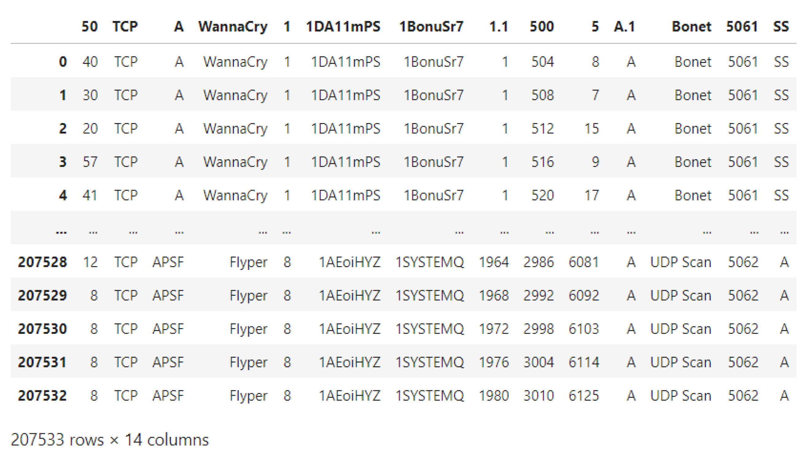
4.1. The UGRansome1819 Dataset
- The category of Synthetic and Signature malware (SS). It represents characteristics of well-known as well as unknown attacks. This category exhibits both, normality and abnormality.
- The category of Signature malware (S). It depicts well-known malware having available keys that have been released and updated regularly. The signature category portrays normality.
- The category of anomaly malware (A). It is a set of unknown malware for which signatures or keys do not yet exist. Abnormality is illustrated by this category.
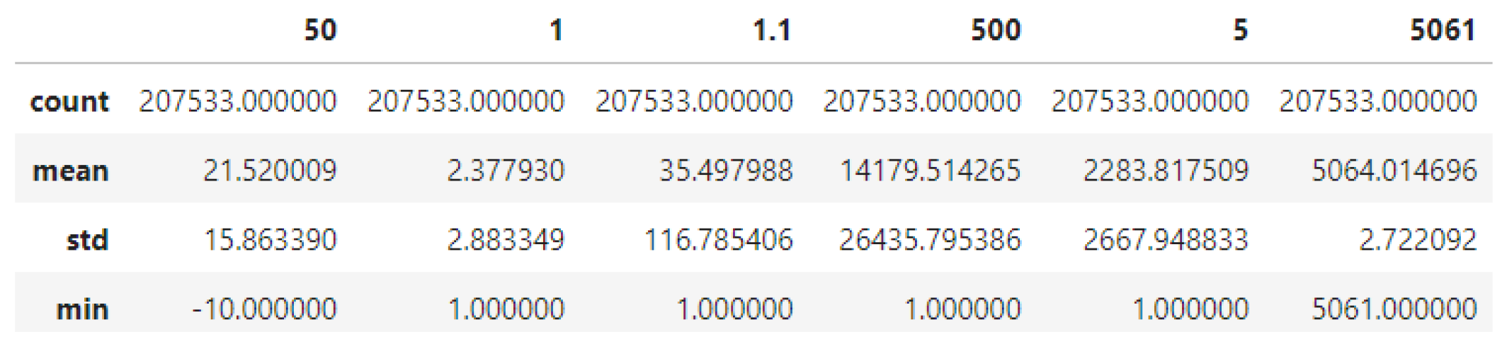
Structure of the Dataset
4.2. Pre-Processing
4.3. Evaluation of the Machine Learning Method
5. Results
5.1. Classification
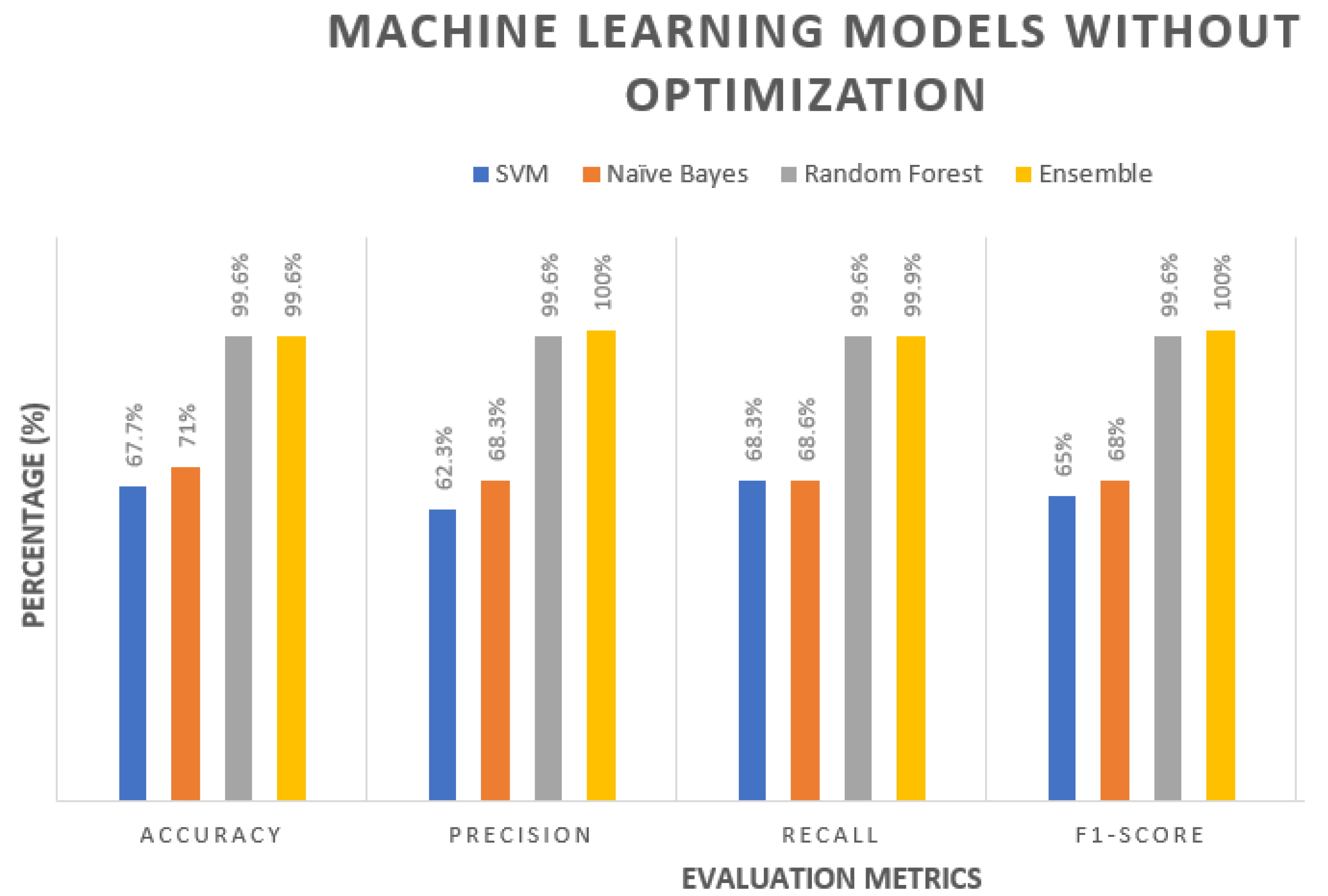
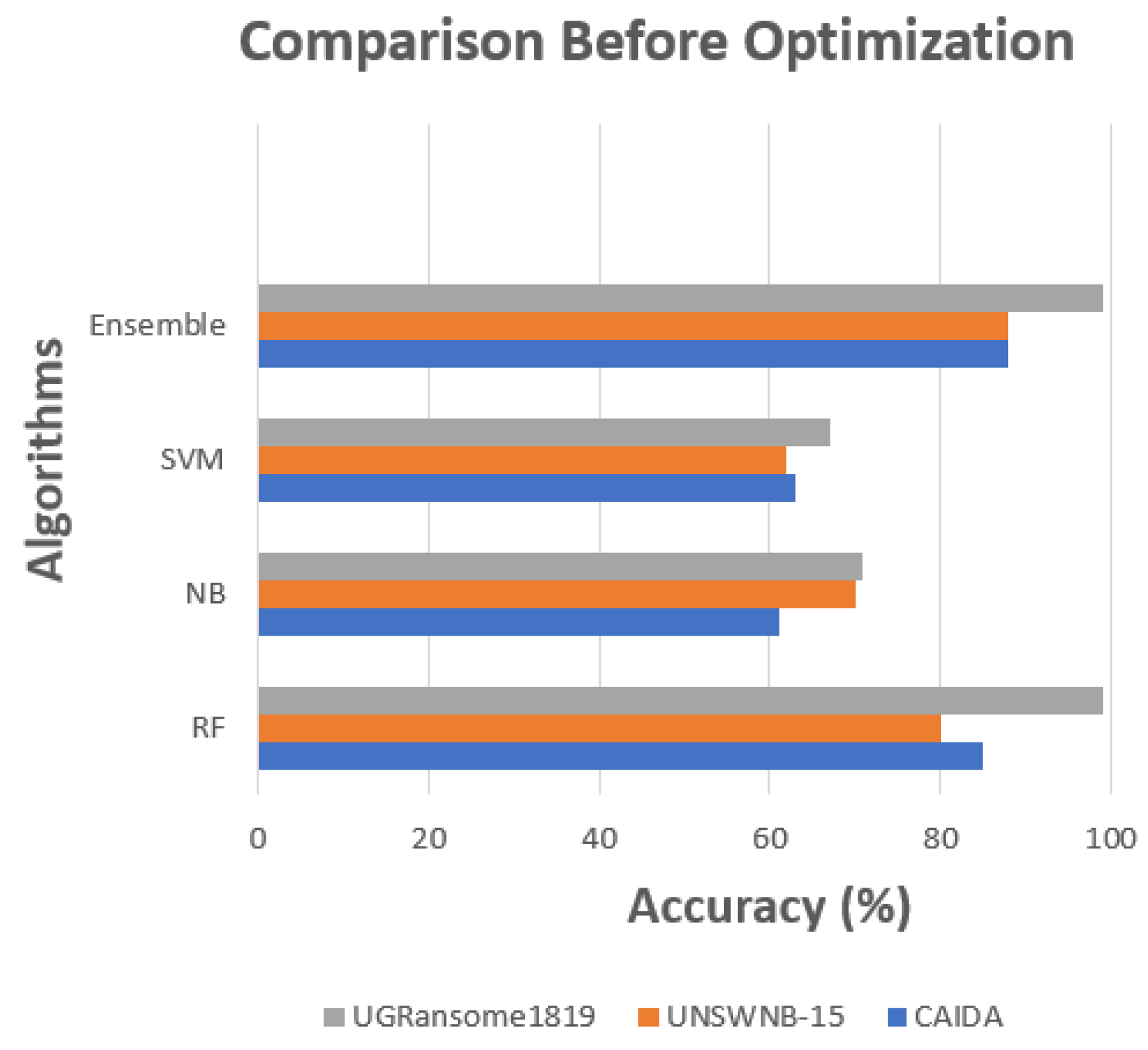
5.2. Without Optimisation
- Use the initial dataset (population) to search
- Calculate the fitness function
- Assess the efficiency of a candidate solution using the fitness function
- Compute the crossover process
- Implement the mutation process
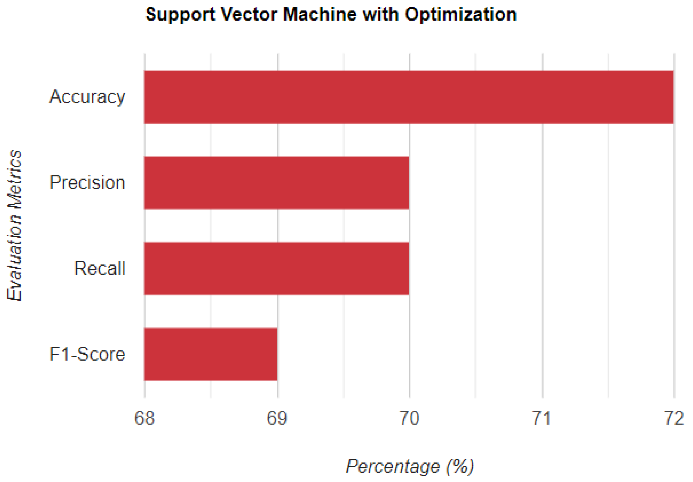
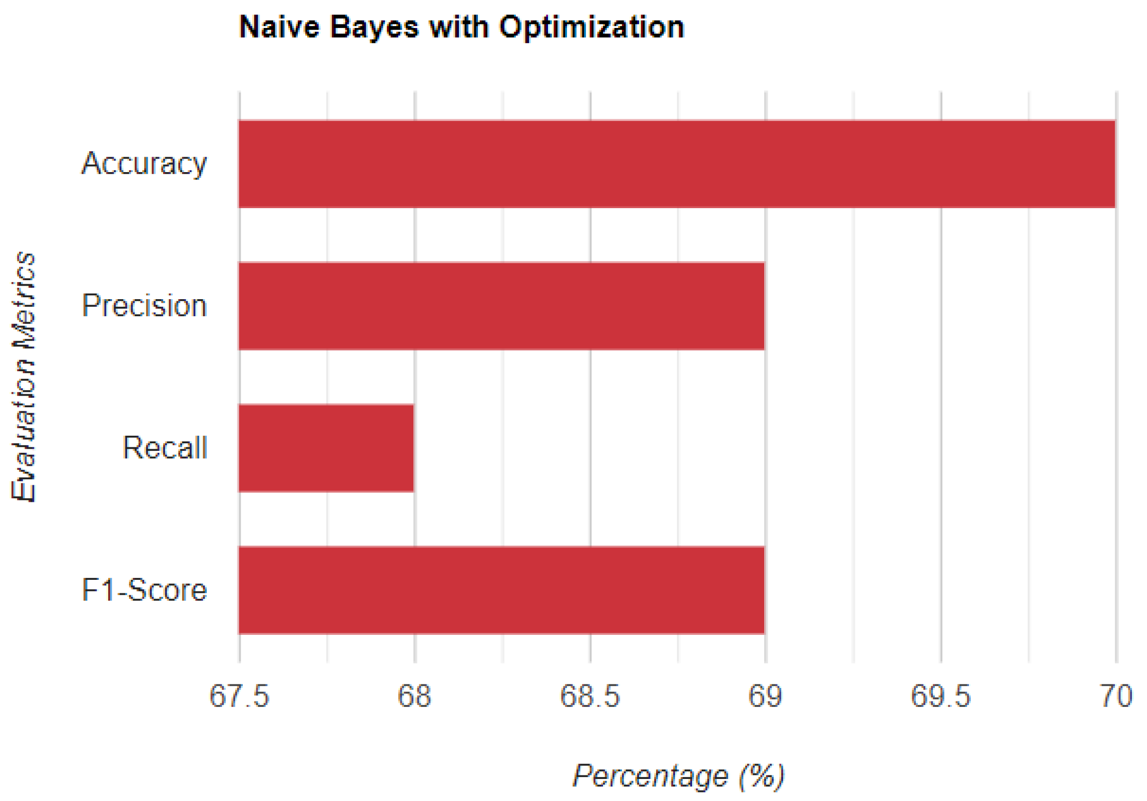
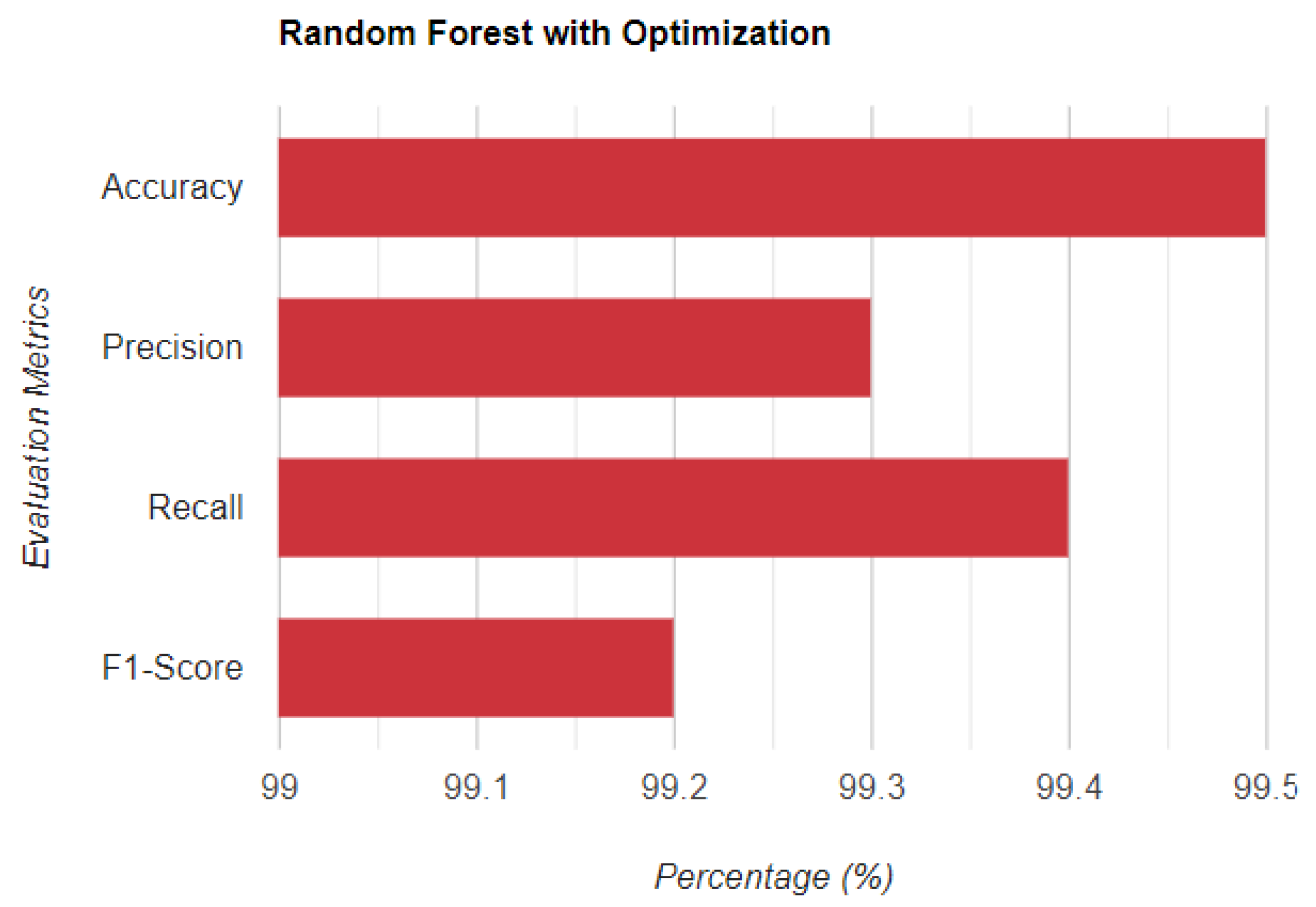
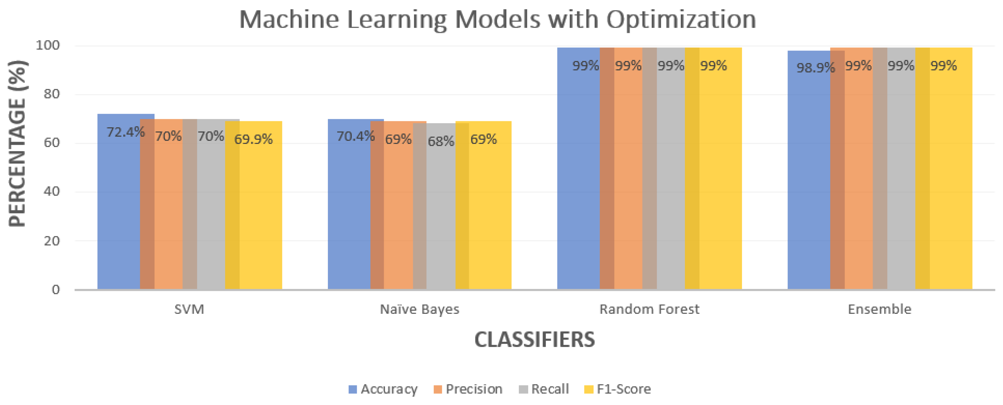
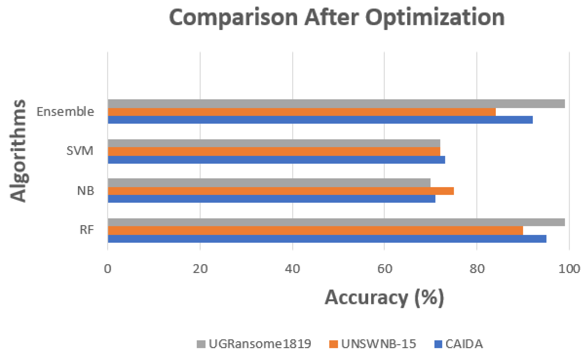
5.3. With Optimization
6. Discussion
7. Conclusions
Author Contributions
Funding
Institutional Review Board Statement
Informed Consent Statement
Data Availability Statement
Conflicts of Interest
References
- Abdelrahman, A.M.; Rodrigues, J.J.; Mahmoud, M.M.; Saleem, K.; Das, A.K.; Korotaev, V.; Kozlov, S.A. Software-defined networking security for private data center networks and clouds: Vulnerabilities, attacks, countermeasures, and solutions. Int. J. Commun. Syst. 2021, 34, e4706. [Google Scholar] [CrossRef]
- Sharafaldin, I.; Gharib, A.; Lashkari, A.H.; Ghorbani, A.A. Towards a reliable intrusion detection benchmark dataset. Softw. Netw. 2018, 2018, 177–200. [Google Scholar] [CrossRef]
- Cordero, C.G.; Vasilomanolakis, E.; Wainakh, A.; Mühlhäuser, M.; Nadjm-Tehrani, S. On generating network traffic datasets with synthetic attacks for intrusion detection. ACM Trans. Priv. Secur. (TOPS) 2021, 24, 1–39. [Google Scholar] [CrossRef]
- Kasongo, S.M.; Sun, Y. A deep learning method with wrapper based feature extraction for wireless intrusion detection system. Comput. Secur. 2020, 92, 101752. [Google Scholar] [CrossRef]
- Dang, Q.V.; Vo, T.H. Studying the Reinforcement Learning techniques for the problem of intrusion detection. In Proceedings of the 2021 4th International Conference on Artificial Intelligence and Big Data (ICAIBD), Chengdu, China, 28–31 May 2021; pp. 87–91. [Google Scholar]
- Vigna, G.; Kemmerer, R.A. NetSTAT: A network-based intrusion detection approach. In Proceedings of the 14th Annual Computer Security Applications Conference (Cat. No. 98EX217), Phoenix, AZ, USA, 7–11 December 1998; pp. 25–34. [Google Scholar]
- Nkongolo, M.; van Deventer, J.P.; Kasongo, S.M. UGRansome1819: A Novel Dataset for Anomaly Detection and Zero-Day Threats. Information 2021, 12, 405. [Google Scholar] [CrossRef]
- Otoum, Y.; Nayak, A. AS-IDS: Anomaly and Signature Based IDS for the Internet of Things. J. Netw. Syst. Manag. 2021, 29, 1–26. [Google Scholar] [CrossRef]
- Ashoor, A.S.; Gore, S. Importance of intrusion detection system (IDS). Int. J. Sci. Eng. Res. 2011, 2, 1–4. [Google Scholar]
- Hindy, H.; Brosset, D.; Bayne, E.; Seeam, A.K.; Tachtatzis, C.; Atkinson, R.; Bellekens, X. A taxonomy of network threats and the effect of current datasets on intrusion detection systems. IEEE Access 2020, 8, 104650–104675. [Google Scholar] [CrossRef]
- Liao, H.J.; Lin, C.H.R.; Lin, Y.C.; Tung, K.Y. Intrusion detection system: A comprehensive review. J. Netw. Comput. Appl. 2013, 36, 16–24. [Google Scholar] [CrossRef]
- Zoppi, T.; Ceccarelli, A.; Bondavalli, A. Unsupervised algorithms to detect zero-day attacks: Strategy and application. IEEE Access 2021, 9, 90603–90615. [Google Scholar] [CrossRef]
- Khraisat, A.; Gondal, I.; Vamplew, P. An anomaly intrusion detection system using C5 decision tree classifier. In Proceedings of the Pacific-Asia Conference on Knowledge Discovery and Data Mining, Melbourne, Australia, 3–6 June 2018; Springer: Cham, Switzerland, 2018; pp. 149–155. [Google Scholar]
- Divekar, A.; Parekh, M.; Savla, V.; Mishra, R.; Shirole, M. Benchmarking datasets for anomaly-based network intrusion detection: KDD CUP 99 alternatives. In Proceedings of the 2018 IEEE 3rd International Conference on Computing, Communication and Security (ICCCS), Kathmandu, Nepal, 25–27 October 2018; pp. 1–8. [Google Scholar]
- Ring, M.; Wunderlich, S.; Scheuring, D.; Landes, D.; Hotho, A. A survey of network-based intrusion detection data sets. Comput. Secur. 2019, 86, 147–167. [Google Scholar] [CrossRef] [Green Version]
- Kilincer, I.F.; Ertam, F.; Sengur, A. Machine learning methods for cyber security intrusion detection: Datasets and comparative study. Comput. Netw. 2021, 188, 107840. [Google Scholar] [CrossRef]
- Lu, S.; Wei, X.; Li, Y.; Wang, L. Detecting anomaly in big data system logs using convolutional neural network. In Proceedings of the 2018 IEEE 16th International Conference on Dependable, Autonomic and Secure Computing, 16th International Conference on Pervasive Intelligence and Computing, 4th International Conference on Big Data Intelligence and Computing and Cyber Science and Technology Congress (DASC/PiCom/DataCom/CyberSciTech), Athens, Greece, 12–15 August 2018; pp. 151–158. [Google Scholar]
- Du, M.; Li, F.; Zheng, G.; Srikumar, V. Deeplog: Anomaly detection and diagnosis from system logs through deep learning. In Proceedings of the 2017 ACM SIGSAC Conference on Computer and Communications Security, Dallas, TX, USA, 30 October–3 November 2017; pp. 1285–1298. [Google Scholar]
- Nkongolo, M.; van Deventer, J.P.; Kasongo, S.M.; van der Walt, W. Classifying Social Media Using Deep Packet Inspection Data. In Proceedings of the 6th International Conference on Inventive Communication and Computational Technologies, Namakkal, India, 12–13 May 2022; Springer: Singapore, 2022; pp. 729–884. [Google Scholar]
- Yu, X.; Joshi, P.; Xu, J.; Jin, G.; Zhang, H.; Jiang, G. Cloudseer: Workflow monitoring of cloud infrastructures via interleaved logs. ACM SIGARCH Comput. Archit. News 2016, 44, 489–502. [Google Scholar] [CrossRef]
- Alazab, A.; Hobbs, M.; Abawajy, J.; Alazab, M. Using feature selection for intrusion detection system. In Proceedings of the 2012 International Symposium on Communications and Information Technologies (ISCIT), Gold Coast, Australia, 2–5 October 2012; pp. 296–301. [Google Scholar]
- Lawal, M.A.; Shaikh, R.A.; Hassan, S.R. An anomaly mitigation framework for iot using fog computing. Electronics 2020, 9, 1565. [Google Scholar] [CrossRef]
- Shapoorifard, H.; Shamsinejad, P. Intrusion detection using a novel hybrid method incorporating an improved KNN. Int. J. Comput. Appl 2017, 173, 5–9. [Google Scholar] [CrossRef]
- Paquet-Clouston, M.; Haslhofer, B.; Dupont, B. Ransomware payments in the bitcoin ecosystem. J. Cybersecur. 2019, 5, tyz003. [Google Scholar] [CrossRef]
- Maseer, Z.K.; Yusof, R.; Bahaman, N.; Mostafa, S.A.; Foozy, C.F.M. Benchmarking of machine learning for anomaly based intrusion detection systems in the CICIDS2017 dataset. IEEE Access 2021, 9, 22351–22370. [Google Scholar] [CrossRef]
- Dong, S. Multi class SVM algorithm with active learning for network traffic classification. Expert Syst. Appl. 2021, 176, 114885. [Google Scholar] [CrossRef]
- Guezzaz, A.; Benkirane, S.; Azrour, M. A Novel Anomaly Network Intrusion Detection System for Internet of Things Security. In IoT and Smart Devices for Sustainable Environment; Springer: Cham, Switzerland, 2022; pp. 129–138. [Google Scholar]
- Li, W.; Li, Q. Using naive Bayes with AdaBoost to enhance network anomaly intrusion detection. In Proceedings of the 2010 Third International Conference on Intelligent Networks and Intelligent Systems, Shenyang, China, 1–3 November 2010; pp. 486–489. [Google Scholar]
- Gattineni, P.; Dharan, G.S. Intrusion Detection Mechanisms: SVM, random forest, and extreme learning machine (ELM). In Proceedings of the 2021 Third International Conference on Inventive Research in Computing Applications (ICIRCA), Shenyang, China, 1–3 November 2010; pp. 273–276. [Google Scholar]
- Disha, R.A.; Waheed, S. Performance analysis of machine learning models for intrusion detection system using Gini Impurity-based Weighted Random Forest (GIWRF) feature selection technique. Cybersecurity 2022, 5, 1–22. [Google Scholar] [CrossRef]
- Yin, C.; Zhu, Y.; Fei, J.; He, X. A deep learning approach for intrusion detection using recurrent neural networks. IEEE Access 2017, 5, 21954–21961. [Google Scholar] [CrossRef]
- Abu Al-Haija, Q.; Al-Badawi, A. Attack-Aware IoT Network Traffic Routing Leveraging Ensemble Learning. Sensors 2022, 22, 241. [Google Scholar] [CrossRef]
- Gaikwad, D.; Thool, R.C. Intrusion detection system using bagging ensemble method of machine learning. In Proceedings of the 2015 International Conference on Computing Communication Control and Automation, Pune, India, 26–27 February 2015; pp. 291–295. [Google Scholar]
- Kasongo, S.M. An Advanced Intrusion Detection System for IIoT Based on GA and Tree Based Algorithms. IEEE Access 2021, 9, 113199–113212. [Google Scholar] [CrossRef]
- Onah, J.O.; Abdulhamid, S.M.; Misra, S.; Sharma, M.M.; Rana, N.; Oluranti, J. Genetic Search Wrapper-Based Naïve Bayes Anomaly Detection Model for Fog Computing Environment. In Proceedings of the International Conference on Intelligent Systems Design and Applications, Salem, India, 5 February 2021; Springer: Cham, Switzerland, 2020; pp. 1371–1382. [Google Scholar]
- Yihunie, F.; Abdelfattah, E.; Regmi, A. Applying machine learning to anomaly-based intrusion detection systems. In Proceedings of the 2019 IEEE Long Island Systems, Applications and Technology Conference (LISAT), Farmingdale, NY, USA, 3 May 2019; pp. 1–5. [Google Scholar]
- Xu, L.; Xiong, W.; Zhou, M.; Chen, L. A Continuous Terminal Sliding-Mode Observer-Based Anomaly Detection Approach for Industrial Communication Networks. Symmetry 2022, 14, 124. [Google Scholar] [CrossRef]
- Ahmad, T.; Truscan, D.; Vain, J.; Porres, I. Early Detection of Network Attacks Using Deep Learning. arXiv 2022, arXiv:2201.11628. [Google Scholar]
- Le, T.T.H.; Kim, H.; Kang, H.; Kim, H. Classification and Explanation for Intrusion Detection System Based on Ensemble Trees and SHAP Method. Sensors 2022, 22, 1154. [Google Scholar] [CrossRef]
- Alzaqebah, A.; Aljarah, I.; Al-Kadi, O.; Damaševičius, R. A Modified Grey Wolf Optimization Algorithm for an Intrusion Detection System. Mathematics 2022, 10, 999. [Google Scholar] [CrossRef]
- Liu, G.; Zhao, H.; Fan, F.; Liu, G.; Xu, Q.; Nazir, S. An Enhanced Intrusion Detection Model Based on Improved kNN in WSNs. Sensors 2022, 22, 1407. [Google Scholar] [CrossRef]
- Ahmad, Z.; Shahid Khan, A.; Wai Shiang, C.; Abdullah, J.; Ahmad, F. Network intrusion detection system: A systematic study of machine learning and deep learning approaches. Trans. Emerg. Telecommun. Technol. 2021, 32, e4150. [Google Scholar] [CrossRef]
- Ahmad, A.; Harjula, E.; Ylianttila, M.; Ahmad, I. Evaluation of machine learning techniques for security in SDN. In Proceedings of the 2020 IEEE Globecom Workshops (GC Wkshps), Taipei, Taiwan, 7–11 December 2020; pp. 1–6. [Google Scholar] [CrossRef]
- Jiang, H.; He, Z.; Ye, G.; Zhang, H. Network intrusion detection based on PSO-XGBoost model. IEEE Access 2020, 8, 58392–58401. [Google Scholar] [CrossRef]
- Zhang, C.; Yu, M.; Wang, W.; Yan, F. MArk: Exploiting Cloud Services for Cost-Effective, SLO-Aware Machine Learning Inference Serving. In Proceedings of the 2019 USENIX Annual Technical Conference (USENIX ATC 19), Renton, WA, USA, 10–12 July 2019; pp. 1049–1062. [Google Scholar]
- Rauschmayr, N.; Kumar, V.; Huilgol, R.; Olgiati, A.; Bhattacharjee, S.; Harish, N.; Kannan, V.; Lele, A.; Acharya, A.; Nielsen, J.; et al. Amazon SageMaker debugger: A system for real-time insights into machine learning model training. Proc. Mach. Learn. Syst. 2021, 3, 770–782. [Google Scholar]
- Sahu, S.K.; Mohapatra, D.P.; Rout, J.K.; Sahoo, K.S.; Pham, Q.V.; Dao, N.N. A LSTM-FCNN based multi-class intrusion detection using scalable framework. Comput. Electr. Eng. 2022, 99, 107720. [Google Scholar] [CrossRef]
- Bevish Jinila, Y.; Prayla Shyry, S.; Christy, A. A Multi-component-Based Zero Trust Model to Mitigate the Threats in Internet of Medical Things. In Data Engineering for Smart Systems; Springer: Singapore, 2022; pp. 605–613. [Google Scholar]
- Leng, F.; Zhang, C.-L.; Chen, W.-Y.; Zeng, Y. Attack analysis based on protocol information of Snort rules. J. Comput. Appl. 2022, 178, 14–19. [Google Scholar] [CrossRef]
- Nkongolo, M.; van Deventer, J.P.; Kasongo, S.M. The Application of Cyclostationary Malware Detection Using Boruta and PCA. In Proceedings of the 5th International Conference on Computer Networks and Inventive Communication Technologies (ICCNCT 2022), Coimbatore, India, 1–2 April 2022; Springer: Singapore, 2022; pp. 631–646. [Google Scholar]
- Xiao, H.H.; Yang, W.K.; Hu, J.; Zhang, Y.P.; Jing, L.J.; Chen, Z.Y. Significance and methodology: Preprocessing the big data for machine learning on TBM performance. Undergr. Space, 2022; in press. [Google Scholar] [CrossRef]
- Nkongolo, M. Classifying search results using neural networks and anomaly detection. Educor Multidiscip. J. 2018, 2, 102–127. [Google Scholar]
- Kasongo, S.M.; Sun, Y. Performance analysis of intrusion detection systems using a feature selection method on the UNSW-NB15 dataset. J. Big Data 2020, 7, 1–20. [Google Scholar] [CrossRef]
- Ranga, V. On Evaluation of Network Intrusion Detection Systems: Statistical Analysis of CIDDS-001 Dataset Using Machine Le...; Universiti Putra Malaysia Press: Serdang, Malaysia, 2018; pp. 1–35. [Google Scholar]
- Pacheco, Y.; Sun, W. Adversarial Machine Learning: A Comparative Study on Contemporary Intrusion Detection Datasets. In Proceedings of the ICISSP, Toledo, OH, USA, 11–13 February 2021; pp. 160–171. [Google Scholar] [CrossRef]
- Sajja, G.S.; Mustafa, M.; Ponnusamy, R.; Abdufattokhov, S. Machine Learning Algorithms in Intrusion Detection and Classification. Ann. Rom. Soc. Cell Biol. 2021, 25, 12211–12219. [Google Scholar]


| Author | Dataset | Approach | Limitations |
|---|---|---|---|
| [37] | CAIDA | SMO | Anomaly detection |
| [38] | CICIDS2017 | Deep Neural Network | IoT protection |
| [39] | NF-BoT-IoT-v2 | Random Forest | Imbalance data |
| [40] | UNSWNB-15 | GWO | Multi-classification |
| [41] | WSN-DS | KNN | Optimization |
| Component | Specification |
|---|---|
| Dataset | UGRansome1819 |
| Processor | 2.60 GHz and 2.59 GHz |
| System Type | 64-bit |
| Programming Language | Python |
| CPU | Intel (R) Core (TM) i7-10 750 |
| OS | Debian 11 |
| Optimization | GA and Ensemble Learning |
| Cloud Services | S3 bucket and SageMaker |
| RAM | 40 GB |
| Abnormal Threats | Example | Prediction | Total |
|---|---|---|---|
| DMALocker | Port Scanning | Anomaly | 12,371 |
| Globe | UDP Scan | Anomaly | 13,200 |
| CryptoLocker Types | Blacklist | Signature | 20,527 |
| JigSaw | Scan | Anomaly | 17,544 |
| SamSam | Spam | Anomaly | 28,597 |
| TowerWeb | Spam | Anomaly | 7353 |
| Flyper | Nerisbonet | Synthetic Signature | 14,352 |
| WannaCry | Bonet | Synthetic Signature | 22,931 |
| APT | DoS | Synthetic Signature | 15,363 |
| Locky | DoS | Synthetic Signature | 33,870 |
| Razy | Scan | Anomaly | 12,535 |
| EDA2 | Blacklist | Signature | 8744 |
| Globev3 | Spam | Anomaly | 146 |
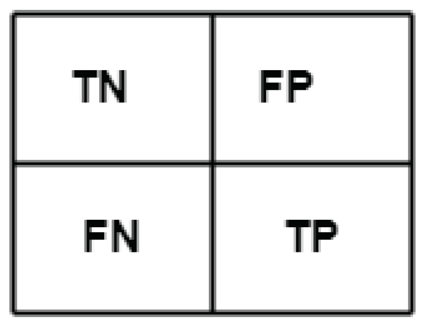
| Accuracy | Precision | Recall | F1-Score |
|---|---|---|---|
| Parameter | Shape |
|---|---|
| Test set | 20% |
| Random state | 42 |
| Train set | 80% |
| Algorithm | Linear SVC |
| Parameter | Shape |
|---|---|
| Test set | 20% |
| Random state | 42 |
| Train set | 80% |
| Algorithm | Gaussian NB |
| Parameter | Shape |
|---|---|
| Test set | 20% |
| Random state | 42 |
| Train set | 80% |
| Algorithm | RF |
| Trees | 100 |
| Parameter | Shape |
|---|---|
| Test set | 20% |
| Base model | NB |
| Train set | 80% |
| Random state | 42 |
| Member model 1 | SVM |
| Member model 2 | RF |
| Algorithm | Stacking |
| Dataset | RF | NB | SVM | Ensemble |
|---|---|---|---|---|
| CAIDA | 85% | 61.8% | 63.2% | 88% |
| UNSWNB-15 | 80% | 70% | 62.4% | 88.2% |
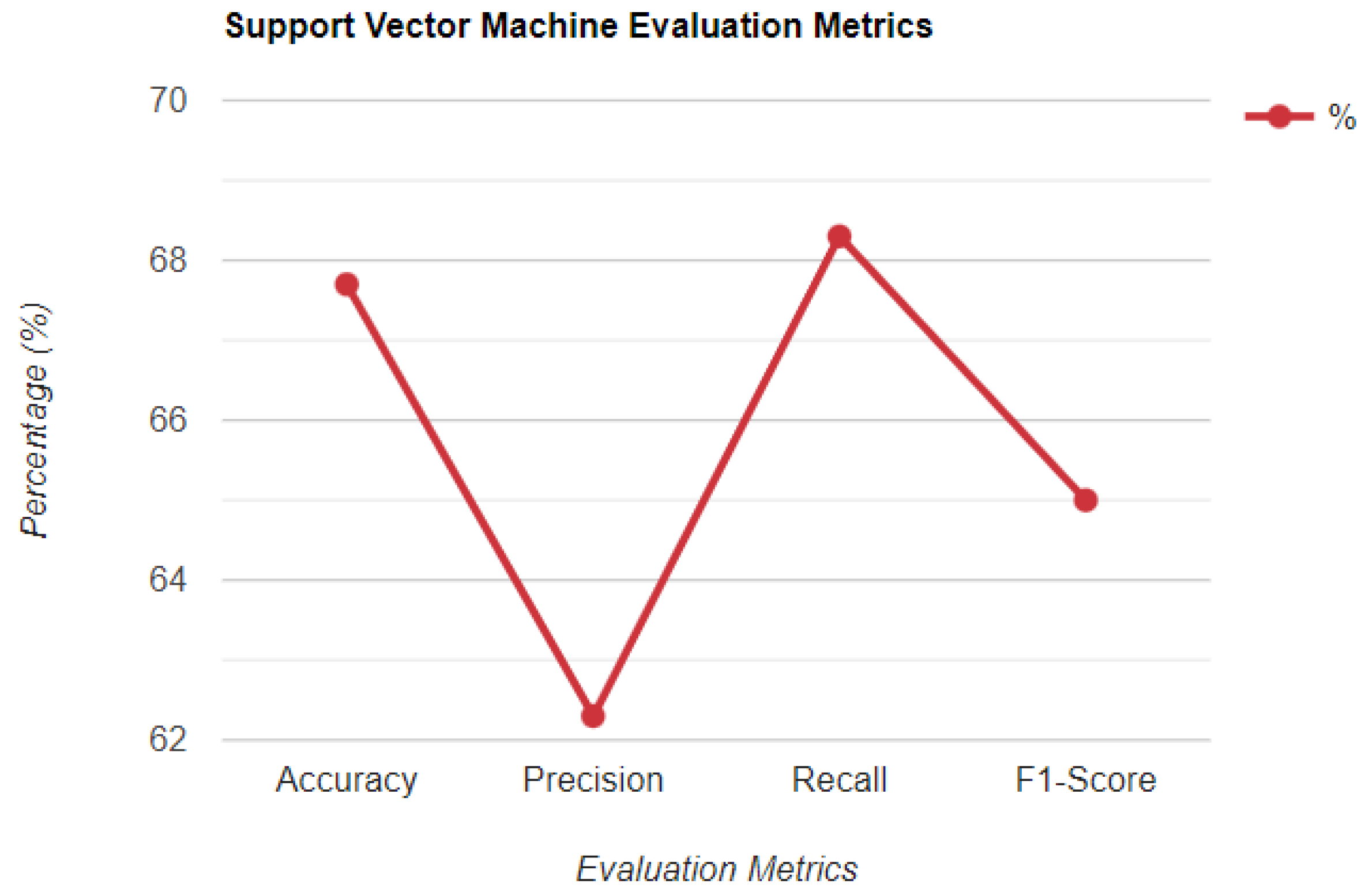
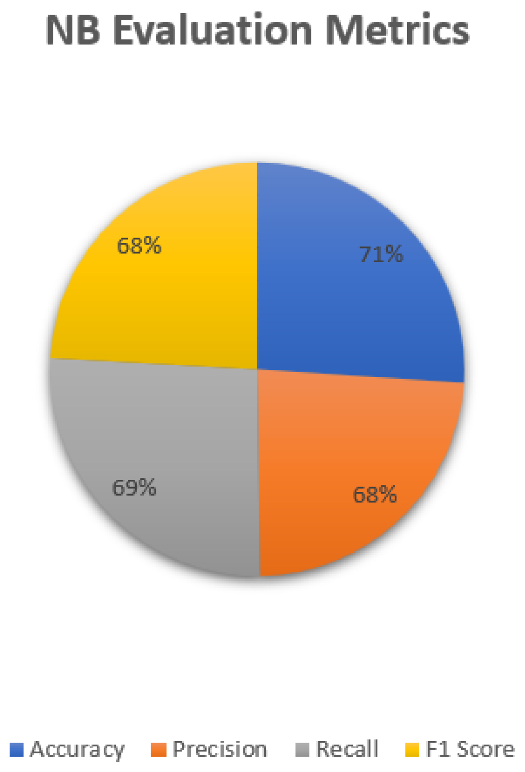
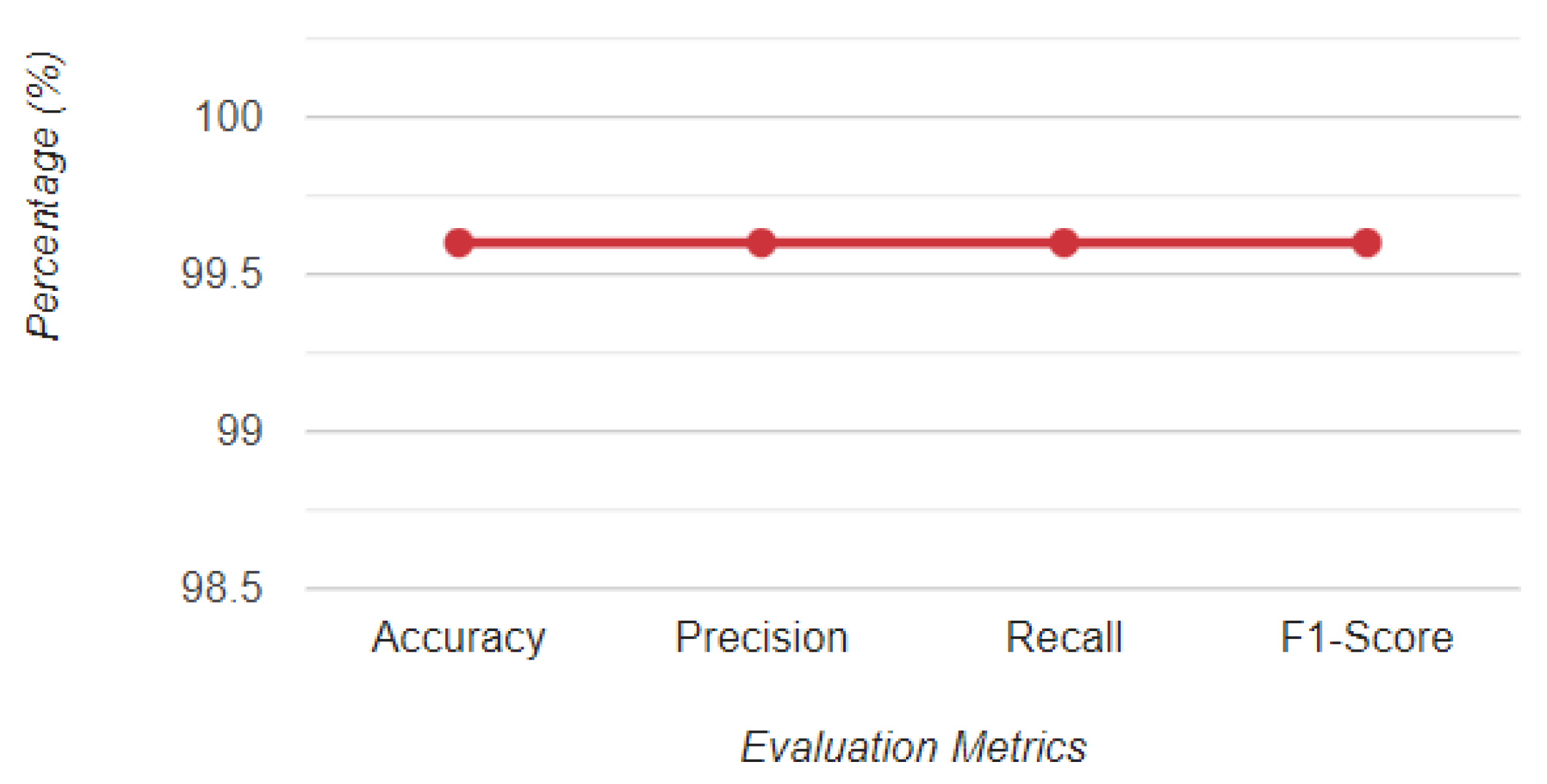
| UGRansome1819 | 99.6% | 71% | 67% | 99.6% |
| Dataset | RF | NB | SVM | Ensemble |
|---|---|---|---|---|
| CAIDA | 95.6% | 71.2% | 73.7% | 92.5% |
| UNSWNB-15 | 90.3% | 75.1% | 72.4% | 84% |
| UGRansome1819 | 99% | 70.4% | 72.4% | 99% |
Publisher’s Note: MDPI stays neutral with regard to jurisdictional claims in published maps and institutional affiliations. |
© 2022 by the authors. Licensee MDPI, Basel, Switzerland. This article is an open access article distributed under the terms and conditions of the Creative Commons Attribution (CC BY) license (https://creativecommons.org/licenses/by/4.0/).
Share and Cite
Nkongolo, M.; Van Deventer, J.P.; Kasongo, S.M.; Zahra, S.R.; Kipongo, J. A Cloud Based Optimization Method for Zero-Day Threats Detection Using Genetic Algorithm and Ensemble Learning. Electronics 2022, 11, 1749. https://doi.org/10.3390/electronics11111749
Nkongolo M, Van Deventer JP, Kasongo SM, Zahra SR, Kipongo J. A Cloud Based Optimization Method for Zero-Day Threats Detection Using Genetic Algorithm and Ensemble Learning. Electronics. 2022; 11(11):1749. https://doi.org/10.3390/electronics11111749
Chicago/Turabian StyleNkongolo, Mike, Jacobus Philippus Van Deventer, Sydney Mambwe Kasongo, Syeda Rabab Zahra, and Joseph Kipongo. 2022. "A Cloud Based Optimization Method for Zero-Day Threats Detection Using Genetic Algorithm and Ensemble Learning" Electronics 11, no. 11: 1749. https://doi.org/10.3390/electronics11111749