Article

Low Frequency Stability of AC Railway Traction Power Systems: Analysis of the Influence of Traction Unit Parameters

1
Department of Electrical, Computer & System Engineering, University of Oviedo, 33204 Gijón, Spain
2
LAPLACE, Université de Toulouse, CNRS, INPT, UPS, 31000 Toulouse, France
3
Ingeteam Power Technology S.A., Traction R&D, 48170 Zamudio, Spain
*
Author to whom correspondence should be addressed.
Electronics 2022, 11(10), 1593; https://doi.org/10.3390/electronics11101593
Submission received: 14 February 2022 / Revised: 23 April 2022 / Accepted: 6 May 2022 / Published: 17 May 2022
(This article belongs to the Special Issue Railway Traction Power Supply)

Abstract

:
Dynamic interactions between AC railway electrification systems and traction unit power converters can result in low frequency oscillation (LFO) of the contact-line voltage amplitude, which can lead to a power outage of the traction substation and the shutdown of train traffic. Several system parameters can influence the low frequency stability of the railway traction power system, including contact-line length and traction unit parameters such as transformer leakage inductance, DC-link capacitance, control bandwidths and synchronization systems. This paper focuses on the influence of these parameters on the LFO. The methodology is based on a frequency-domain analysis. Nyquist and Bode diagrams are used to determine the stability limit. The validation of the method is performed through the use of time-domain simulations.

1. Introduction

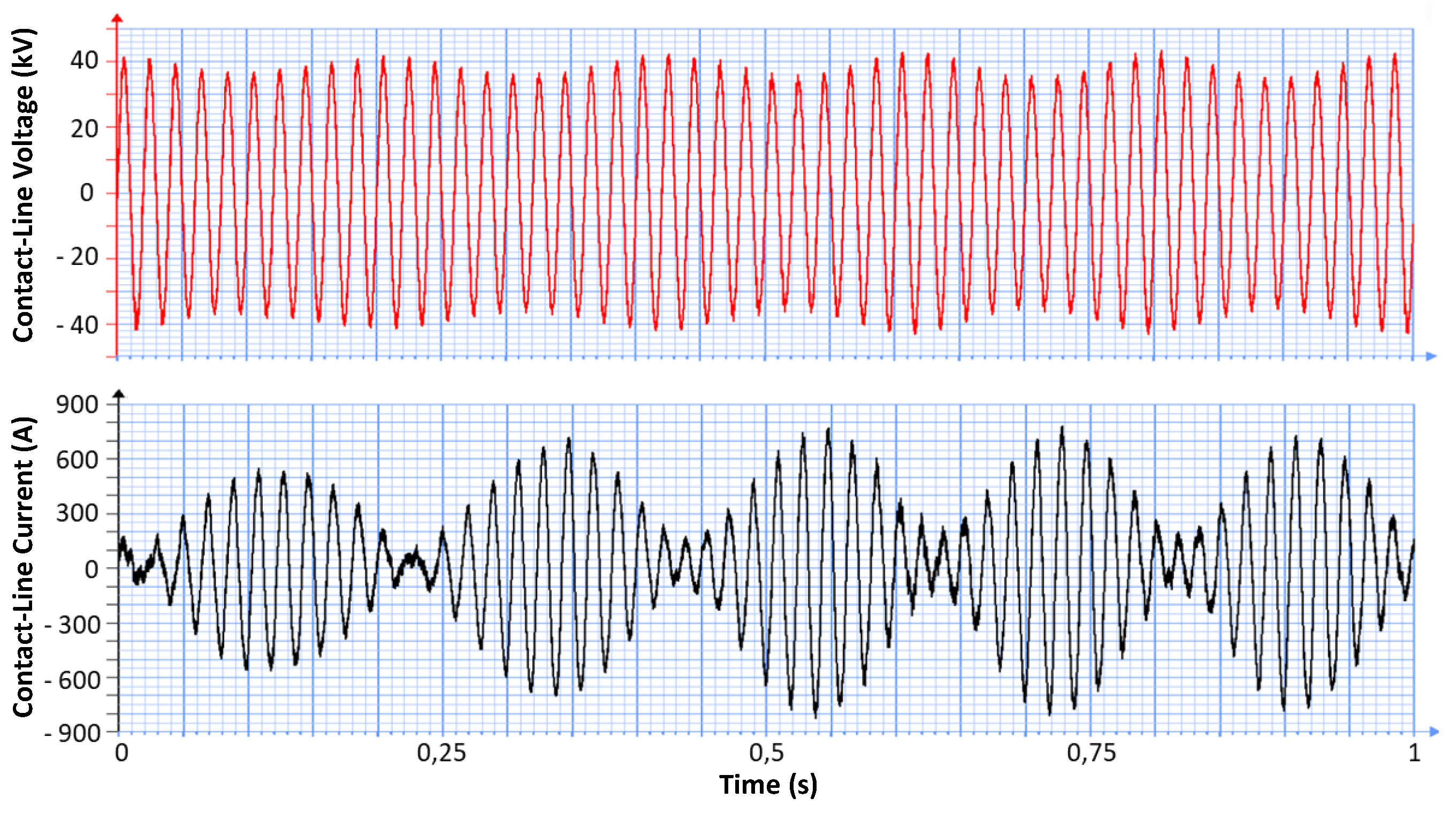
1.1. Review of LFO Events

Modern rail vehicles that operate in the railway system include a large number of power electronic converters aimed to improve performance and efficiency. Despite the benefits, complex dynamic interactions between the railway network and the controlled power converters can produce undesired phenomena, which might result in power system instability, including the LFO phenomenon [1,2,3,4,5,6,7,8], harmonic resonance [8] and electrical resonant instability [9]. The LFO phenomenon has been reported worldwide for different types of railway networks under different operating conditions; see Table 1.
Reported events include a 15 kV/16.7 Hz power system supplied from rotary converters [2], a 12 kV/25 Hz system with static frequency converters [4], and 25 kV/50 Hz power systems supplied from the public grid such as the case observed in the sector of Thionville in France [5], shown in Figure 1.
When LFO occurs, an amplitude modulation of contact-line voltage and current is produced, i.e., the oscillation frequency f o s c is presented in the envelope of the signal waveforms, see Figure 1. This is seen in the frequency spectra of voltage and current as a fundamental frequency component at f 0 along with two sideband components at ( f 0 f o s c ) and ( f 0 + f o s c ) as explained in [10]. From the events reported in Table 1, the oscillation frequencies reached values up to 7 Hz (i.e., 43–57 Hz in the stationary reference frame). This phenomenon has caused a number of serious issues, such as the malfunction of the protection system, over-voltage and over-current, which could damage the electrical/electronic equipment and cause transportation delays [7].
In the railway system, two specific scenarios in which the LFO phenomenon has been reported are: first, multiple trains in the depot (i.e., all the vehicles located at the same place) [5]; second, a train operating at a very long distance from a substation [3]. From the point of view of the stability analysis, these two scenarios are equivalent, as will be explained in Section 3.1, using the impedance-based small-signal model [6,11,12]. The study presented is applicable to both scenarios. An analysis for multiple trains in different positions of the contact-line is out of the scope of this article, but it should be taken into account for further research. The 25 kV/50 Hz power supply system is considered.

1.2. Content and Contribution

This paper analyzes the influence of some constructive and operational parameters that may contribute to low frequency instability, including contact-line length (i.e., distance from the substation), consumed power on the DC link that supplies the three-phase motor drives, the bandwidth of current and voltage controllers, transformer leakage inductance, DC-link capacitance, synchronization systems and feedforward signals. Since perturbation frequencies are present around f 0 , a stability study is performed using an impedance-based analysis in the frequency-domain on the dq synchronous reference frame [11,13]. The train input admittance in the dq frame required for the stability analysis is obtained using a frequency response test as in [5]. Alternatively, the admittance could be obtained from analytical models as in [7,8]; however, these models have been reported to be not accurate enough [14]. Nyquist and Bode diagrams are used to determine the system stability limit, which is defined as the maximum distance from a substation at which a traction unit can operate safely, or the maximum numbers of traction chains connected in parallel on a specific contact-line sector. This capacity of predicting the stability limit allows to obtain the stability limit curve (SLC) in the complex impedance plane ( R , X ) [11]. This curve is plotted for a specific traction chain, and it is useful to find the stability limit in any railway traction system. The method for stability analysis used in this article is validated with the use of time-domain simulations. PLECS Blockset software along with MATLAB/Simulink were used for the frequency-domain analysis and for time-domain simulations.
This type of study using frequency-domain stability analysis has not been reported in the literature before; a similar approach of parameter variations study has been performed partially by [4,10] but using eigenvalue migration. Furthermore, in this paper, different types of synchronization systems and some methods to generate the feedforward signal have been considered in a comparison study, which results in a new contribution in the field of low frequency stability.

1.3. Organization

The paper is organized as follows. Section 2 describes the railway traction system model and the control system. Section 3 presents the stability analysis in the frequency-domain for the study of the LFO phenomenon. Section 4 studies the influence of contact-line length; three different cases are studied, and validation of the analysis is performed through simulations. Section 5 deals with the impact of the power consumption on the DC link, stability and limits are calculated for a specific contact-line. Section 6 addresses the combined effect of transformer leakage inductance and current controller parameters. Section 7 deals with the influence of the DC-link capacitor and the voltage controller bandwidth. Section 8 studies the characteristics of the phase-locked loop (PLL) and the impact of the feedforward signal, and four combined cases are considered. Finally, conclusions are drawn in Section 9.

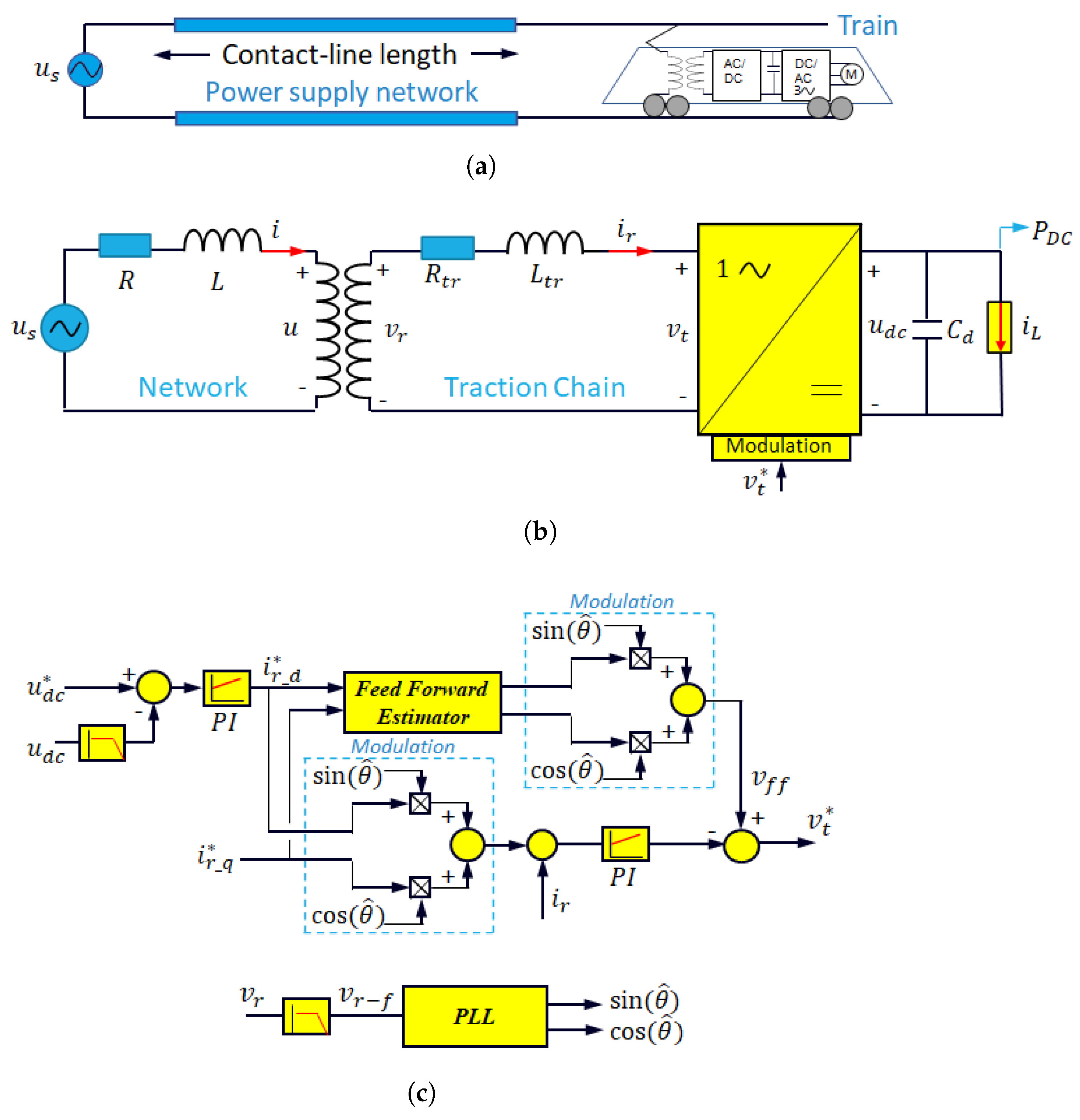
2. Railway Traction System Model for LFO Phenomenon Study

A schematic representation of the railway traction system is shown in Figure 2a. It consists of two main blocks: the power supply network and the traction unit that consists of one or more traction chains [15]. The power supply network is composed of an ideal voltage source at a fixed frequency, the impedance of the substation transformer and the impedance of the contact-line (i.e., transmission line).
An analytical calculation of contact-line impedance performed in [16] using transmission line equations shows that at frequencies around the fundamental frequency f 0 = 50 Hz, the contact-line can be approached by an inductive-resistive (RL) element. Capacitive effects would only appear at high frequencies, and could be therefore safely neglected. The simplified RL model is also supported by the experience reported in [1,6,7,12,16], and also is considered in the European standard document for the compatibility of rolling stock and infrastructure EN-50388-2 [17]. Consistently with the previous discussion, Figure 2b shows the main elements of the simplified railway traction system model used for this study, which consists of a single traction chain and an equivalent circuit of the power supply that only considers a resistance (R) and an inductance (L).
The main elements in the traction chain are: an input transformer with its leakage inductance ( L t r ) and winding resistance ( R t r ); a single-phase four-quadrant power converter (4QC); a DC-link capacitor ( C d ); and traction drives consisting of inverters and motors. In this study, traction drives are modeled as an equivalent current source.
Figure 2c shows the traction chain control system. Two cascaded loops regulate the voltage of the DC link (slow regulation) and the absorbed current at the contact-line (fast regulation) using proportional-integral (PI) regulators [13]. This inner loop is improved with a feedforward estimator that anticipates the voltage drop across the input transformer impedance [13]. To guarantee a power factor close to unity, system synchronization is performed using the estimated contact-line voltage phase angle ( θ ^ ), which is calculated using a PLL. This angle is used for coordinate transformation between the stationary reference frame and the synchronous reference frame (i.e., dq frame). Independent control of active and reactive power using the currents I d and I q can be achieved.
In order to obtain the desired current control bandwidth ( ω b c c ) and voltage control bandwidth ( ω b v c ), controllers (i.e., k p c c , k i c c , k p v c , k i v c ) were tuned using Equations (1) and (2) as described in [13].
k p c c = L t r · ω b c c , k i c c = L t r · ω b c c 2 π ,
k p v c = C d · ω b v c , k i v c = C d · ω b v c 2 π

3. Impedance-Based Stability Analysis for the Study of the Low Frequency Oscillations Phenomenon

This section describes the use of the frequency-domain stability criteria applied to the impedance-based small-signal model of the railway traction system, aimed to determine the risk of LFO instability. This small-signal model covers the study of the LFO phenomenon reported for multiple trains located at the same place (e.g., trains at depot) and for the case of a train operating at a very long distance from a substation. For both scenarios, the stability study could be performed considering an equivalent case that only takes into account the interaction between a multiple value of the power supply base impedance and a single traction chain.

3.1. Impedance-Based Small-Signal Model

The small-signal model of the traction railway system in the frequency-domain, developed and presented in [2,6,9,12], is shown in Figure 3a, where U s is the no-load voltage at the substation, U is the contact-line voltage, I is the contact-line current, Z s is the base network impedance, n is a multiplicative factor of base impedance, Y t is the admittance of a traction chain, and m is the number of traction chains. Additionally, it is important to define Z = n Z s as the total network impedance (i.e., power supply impedance) that includes the upstream grid impedance, the substation impedance and the contact-line impedance. The total input admittance is Y = m Y t . The delta symbol ( Δ ) refers to the small variations of the variables around a specific operating point at which the small-signal analysis will be performed. Figure 3 shows that the railway traction small-signal model can be represented as a closed-loop system, whose transfer function G ( j ω ) = Δ I / Δ U s is given by Equation (3).
G ( j ω ) = m Y t 1 + n m Y t Z s = Y 1 + Y Z
The denominator of Equation (3) is called the characteristic equation [18], which should not be equal to zero for any frequency in order to guarantee system stability [5]. From the point of view of the stability analysis the multiple number of the base impedance that composes the overhead line (n) and the number of traction chains (m) are interchangeable terms, meaning that m · n will be a critical coefficient of the characteristic equation. Therefore, a system composed of a number of identical traction chains is equivalent to a system with a single traction chain fed through a multiple of the power base impedance; for instance, the case ( n = 1 , m = 4 ) has the same characteristic equation as the case ( n = 4 , m = 1 ) . For the sake of simplicity, in this article n = m = 1 will be assumed unless otherwise stated.

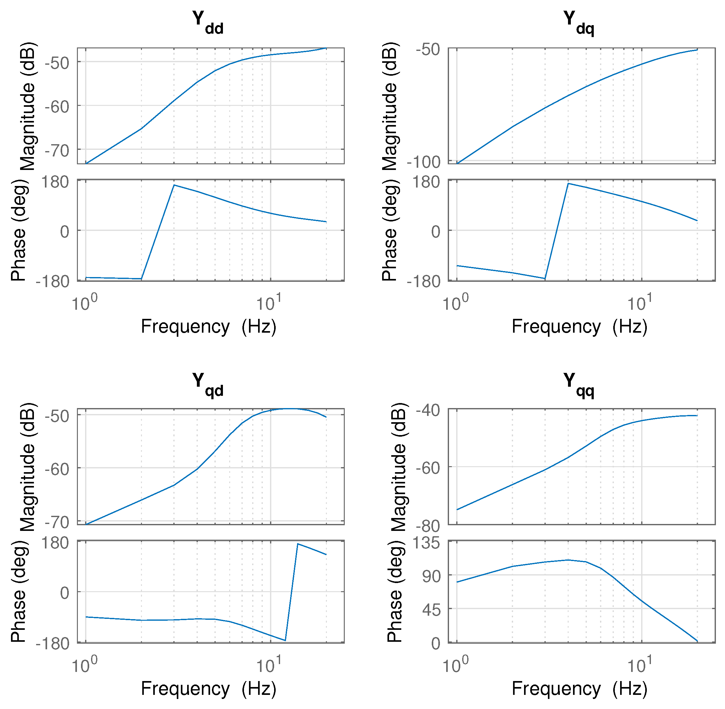
3.2. Network Impedance and Traction-Chain Admittance

As explained in Section 2, the control system of the traction chain considers a dq reference frame aligned to the contact-line voltage that allows independent control of active and reactive power using the currents I d and I q , respectively. Therefore, the power supply and the traction chain form a multiple-input and multiple-output (MIMO) system in the dq reference frame.
Equation (4) shows the network impedance matrix in the dq reference frame [12,19], which is expressed in terms of the network resistance, R, the network inductance, L, the fundamental angular frequency, ω 0 = 2 π f 0 , and the perturbation (i.e., excitation) angular frequency, ω = 2 π f .
Z DQ ( j ω ) = Z d d ( j ω ) Z d q ( j ω ) Z q d ( j ω ) Z q q ( j ω ) = R + j ω L ω 0 L ω 0 L R + j ω L
Equation (7) shows the input admittance matrix of the traction chain that is obtained using the frequency response scanning method described in [5], where small-signal variations in the d sin ( ω 0 t ) and q cos ( ω 0 t ) components of the contact-line voltage, Δ U d and Δ U q , are applied to the traction chain at a certain perturbation angular frequency, ω , see Equation (5). Then, variations of the current components from Equation (6), ( Δ I d , ϕ d ) and ( Δ I q , ϕ q ) , related to each perturbation frequency, are extracted [5,12]. For this study, the perturbation frequencies are in a range up to 20 Hz.
u ( t ) = U d + Δ U d sin ( ω t ) sin ( ω 0 t ) + Δ U q sin ( ω t ) cos ( ω 0 t )
i ( t ) = I d + Δ I d sin ( ω t + ϕ d ) sin ( ω 0 t ) + I q + Δ I q sin ( ω t + ϕ q ) cos ( ω 0 t )
Y DQ ( j ω ) = Y d d ( j ω ) Y d q ( j ω ) Y q d ( j ω ) Y q q ( j ω ) = Δ I d ϕ d Δ U d Δ U q = 0 Δ I d ϕ d Δ U q Δ U d = 0 Δ I q ϕ q Δ U d Δ U q = 0 Δ I q ϕ q Δ U q Δ U d = 0
Examples of the dq admittance matrix are presented in Section 4 and Section 8.

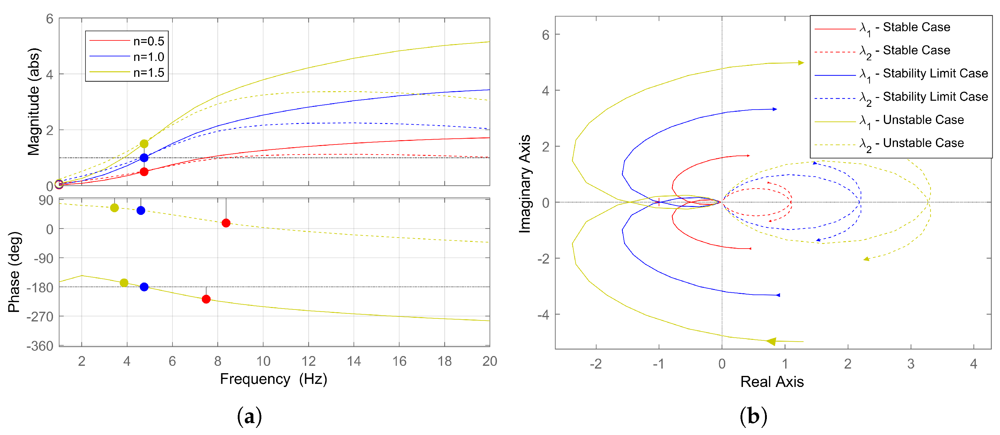
3.3. Stability Criteria

The rail vehicle connected to an ideal power source is considered a stable system [20]. The impedance of the railway power supply network is a passive element (i.e., RL element), which implies it is also stable. Therefore, these two elements are stable in an open loop. Stability criteria for the interconnection of these two elements in a closed loop system are presented in this section for the study of the LFO phenomenon.
A factorization of the system open loop transfer function, L ( j ω ) , is described in Equation (8), where Λ ( j ω ) is the eigenvalue matrix and P is the eigenvector matrix [12,15].
L ( j ω ) = Y DQ ( j ω ) Z DQ ( j ω ) = P Λ ( j ω ) P 1
Λ ( j ω ) = λ 1 ( j ω ) 0 0 λ 2 ( j ω )
From Equation (9), Λ ( j ω ) is presented as a diagonal matrix that allows to study the stability of the eigenvalues λ 1 ( j ω ) and λ 2 ( j ω ) as two decoupled single-input single-output (SISO) systems.
Rever’s criterion applied in a Bode diagram [11] and Nyquist criterion [18] are widely used to analyze the stability of SISO systems in the frequency-domain. Both criteria are equivalent, and either one is used at the authors’ convenience in this paper. These criteria have been selected since they are trusted and verified, and have been employed in previous studies of low frequency stability. Rever’s criterion was selected for the study performed in [12,15], while the Nyquist criterion was used in [6,19,21].
The stability criterion based on Revers specifies that the closed-loop system is stable if, at the crossover frequency f c , at which A r g ( λ 1 , 2 ( j · 2 π · f c ) ) = 180 ° , the module of the open loop transfer function is less than 1 in absolute units (i.e., less than 0 decibels) [11]. In a similar approach, the Nyquist criterion specifies that the closed loop system is stable if the eigenvalues do not encircle the point ( 1 , 180 ° ) in the complex plane [18]. Both criteria are equivalent, and either one is used at the authors’ convenience in this paper.
The gain margin is defined as G M = 1 / λ 1 , 2 ( 2 π f c ) ; therefore, stability is ensured for a gain margin larger than 1 in absolute units (i.e., positive values in db). At point λ 1 , 2 = 1 , the phase margin is defined as PM = ( A r g ( λ 1 , 2 ) ( 180 ° ) ) [18].

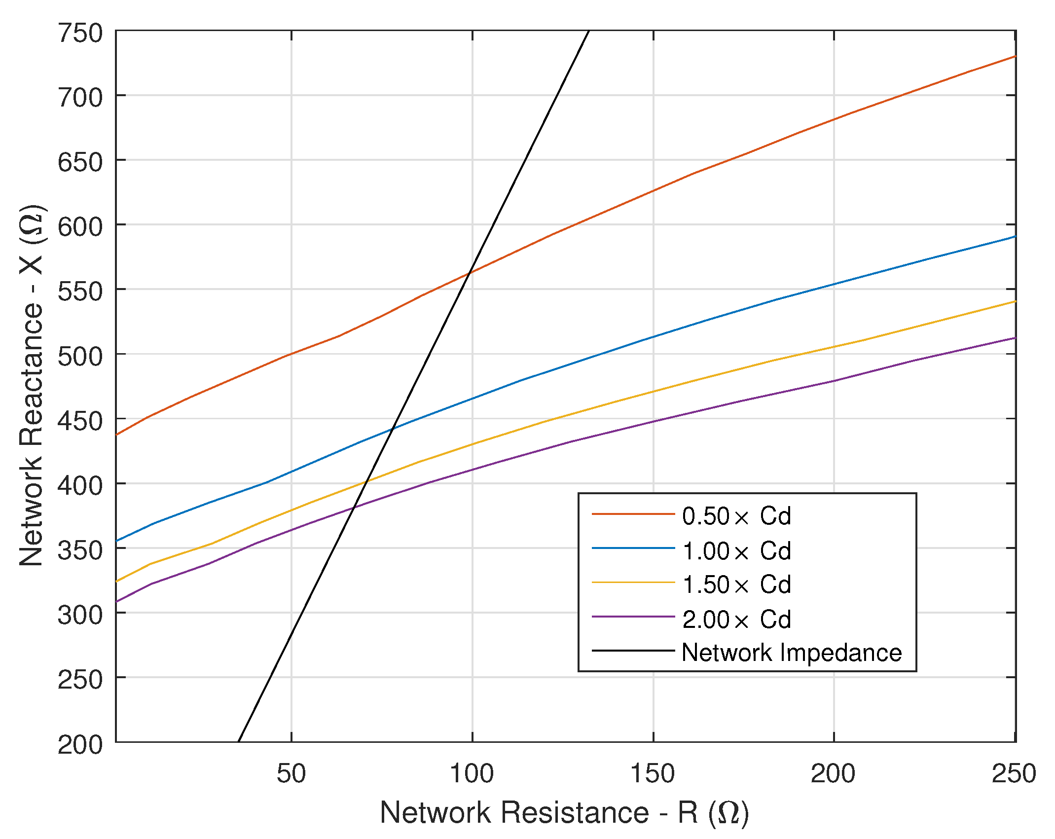
3.4. Stability Limit Curve in the Network Reactance (X) and Resistant (R) Complex Plane

From Section 3.3, the stability limit is reached when any of the eigenvalues is λ 1 , 2 = ( 1 , 180 ° ) = 1 . Thus, for a specific traction chain with an associated input admittance Y DQ , a set of values of network reactance, X, and resistance, R, can be tested to find a curve X = X ( R ) in the complex impedance plane that takes the system to the stability limit as explained in [12]. This curve can be obtained based on an iterative process using three nested loops. The first loop is used to modify the value of R, the next loop modifies the inductance L, and the third loop checks fulfillment of the critical condition of stability by the eigenvalues. As explained in [12], since this iterative process is performed using discrete steps, the following thresholds are defined for the eigenvalues that reach the stability limit:
  • 180 ° < A r g ( λ 1 , 2 ) < 178 °
  • 0.98 < λ 1 , 2 < 1

4. Influence of Contact-Line Length on the Railway Traction System Stability

In this section, the stability criteria described in Section 3 are used. A traction unit connected to a contact-line with different lengths (i.e., different network impedance) is considered. Only one traction chain per traction unit is considered (i.e., m = 1 ). The study presents three different cases: a stable system, a system at its stability limit, and an unstable system. Time-domain simulations will be used to verify the stability analysis performed in the frequency-domain.

4.1. Traction Chain Input Admittance

The dq input admittance of the traction chain is presented in Figure 4. The electrical and control parameters of the traction chain are found in Table 2.

4.2. Network Impedance

The components of the network impedance Z are the upstream grid impedance Z u g , the substation impedance Z s s t , and the contact-line impedance Z c l = d × Z c l , which depends on the distance (d) between the traction unit and the substation (i.e., contact-line length) [12]. See Equation (10).
Z = 2 × Z u g + Z s s t + d × Z c l
The parameters used in this study are the following:
  • Z u g = (0.5 Ω ; 80 ° )
  • Z s s t = (5.5 Ω ; 80 ° )
  • Z c l = (0.5 Ω /km; 80 ° )
The total network line impedance Z = n Z s is used for each case of study, where Z s = (448.1 Ω ; 80 ° ) is the base impedance at the stability limit, which occurs at 883.3 km distance. A value n = 1 corresponds to the stability limit case; n = 0.5 and n = 1.5 will be used as examples for the stable and unstable cases. Here, the distance to reach the stability limit is theoretical [12], and it is much higher than the typical length of a sector (around 50 km). In the 25 kV/50 Hz power supply, all the sectors are electrically isolated and there is one transformer per sector. The theoretical distances are used to facilitate the stability study (i.e., to find the stability limit) since only one traction chain is being considered for the analysis [15], so, for a unit equipped with more than one traction chain, the distance limit is reduced according to the equivalence between n and m, explained in Section 3.1. Considering 50 km as the maximum length of a sector in a 25 kV/50 Hz power supply system and vehicles equipped with four traction chains, the stability limit equivalence occurs when 3.55 vehicles are operating at the end of the sector line.

4.3. Stability Analysis

Using the traction chain input admittance matrix and the network impedance matrix, the system eigenvalues of the open-loop transfer function for the three study cases are calculated from Equation (8); they are shown in Figure 5, where the Bode diagram and the Nyquist plot are used for representation. The marked dots in the Bode diagram identify the gain and phase margins. In the Nyquist plot, the gain margin is the reciprocal absolute value of the intersection point between the eigenvalue curve with the negative real axis.
Increasing the contact-line length increases the gain of the total network impedance but keeps constant its phase. Therefore, the variation of contact-line length modifies only the gain of the eigenvalues λ 1 and λ 2 as shown in Figure 5a.
In the same figure, it is seen that the phase of eigenvalue λ 2 never intersects 180 ° at any frequency, which means that this eigenvalue is not causing instability. This applies to the three study cases. The same conclusion is reached using the Nyquist stability criterion in Figure 5b since λ 2 never encloses −1. For the stable case (red curve), the eigenvalue λ 1 at crossover frequency f c (i.e., crossing phase at 180 ° ) has a magnitude lower than 1, which fulfills the stability criterion explained in Section 3.3. Therefore, for this case, both system eigenvalues guarantee stability.
Increasing the power supply impedance by a factor of two (i.e., n = 0.5 to n = 1 ) will move the eigenvalue from λ 1 ( j 2 π f c ) = ( 0.5 , 180 ° ) to λ 1 ( j 2 π f c ) = ( 1 , 180 ° ) , causing the system to reach the stability limit operational point. Similarly, when the network impedance is increased by a factor n = 1.5 , the eigenvalue will go to λ 1 ( j 2 π f c ) = ( 1.5 , 180 ° ) , see Figure 5a; thus, the system is not fulfilling the stability criterion anymore and the system becomes unstable.
The same analysis can be done using the Nyquist plot from Figure 5b. For the stable case, the eigenvalue λ 1 does not encloses −1, which fulfills the Nyquist stability criterion; however, the eigenvalue λ 1 intersects the negative real axis; therefore, a risk of instability is present when increasing the gain of the critical eigenvalue (i.e., increasing the power supply impedance or the number of traction chains, see the equivalence of n and m explained in Section 3.1).
It is important to notice from Figure 5 that the gain margin is less than 1 when systems are unstable, equals 1 at the stability limit, and takes values greater than 1 when the system is stable, so it can be used as the degree of safety from 1 (i.e., minimum value of safety) to infinite (i.e., best case). The gain margin also indicates the number of network impedance units or traction chains where the system reaches the stability limit. On the other hand, the crossover frequency corresponds to the oscillation frequency at the stability limit.
Time-domain simulations were performed to verify the stability analysis developed in this section. Figure 6 shows the simulation for the operating point of each study case. DC-link voltage, contact-line voltage, and traction chain current are presented. Initially, the system is operating at a stable state close to the substation; then, the power supply impedance is increased in three steps. The first step change of 0.5 · Z s occurs at t = 5 s; here, the system experiences a small oscillation that is damped quickly, and the system is taken again to a stable state. A second step change of 0.5 · Z s in the power supply impedance occurs at t = 6 s, where the time response is oscillatory and no damping is present, but the system is still stable; the oscillation frequencies of the DC-link voltage, the envelope of the contact-line voltage and the current correspond to the oscillation frequency predicted by the impedance-based stability analysis; a frequency around 4.75 Hz can be seen in the figure. Finally, following the increase of the power supply impedance at t = 8 s, the system becomes unstable.

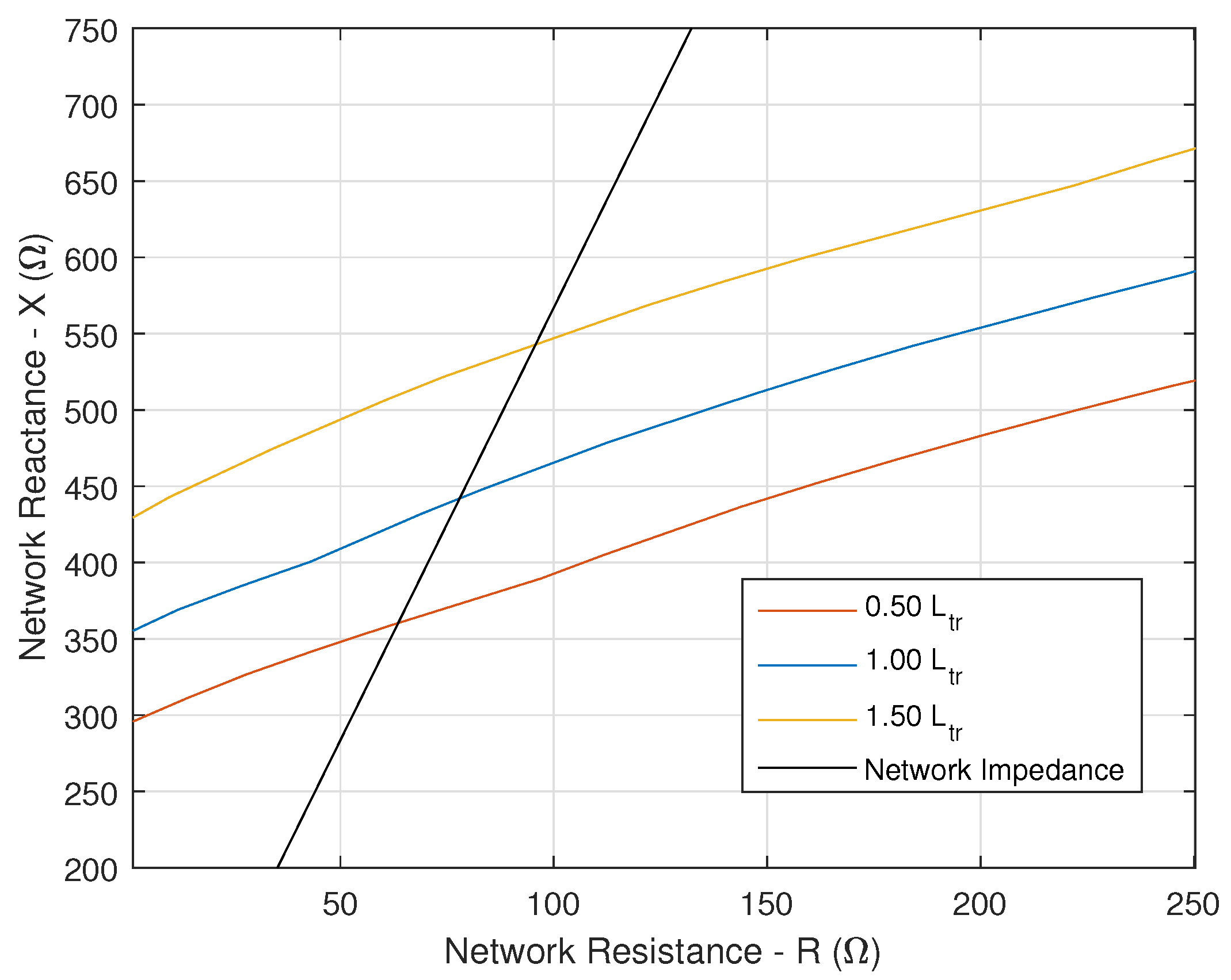
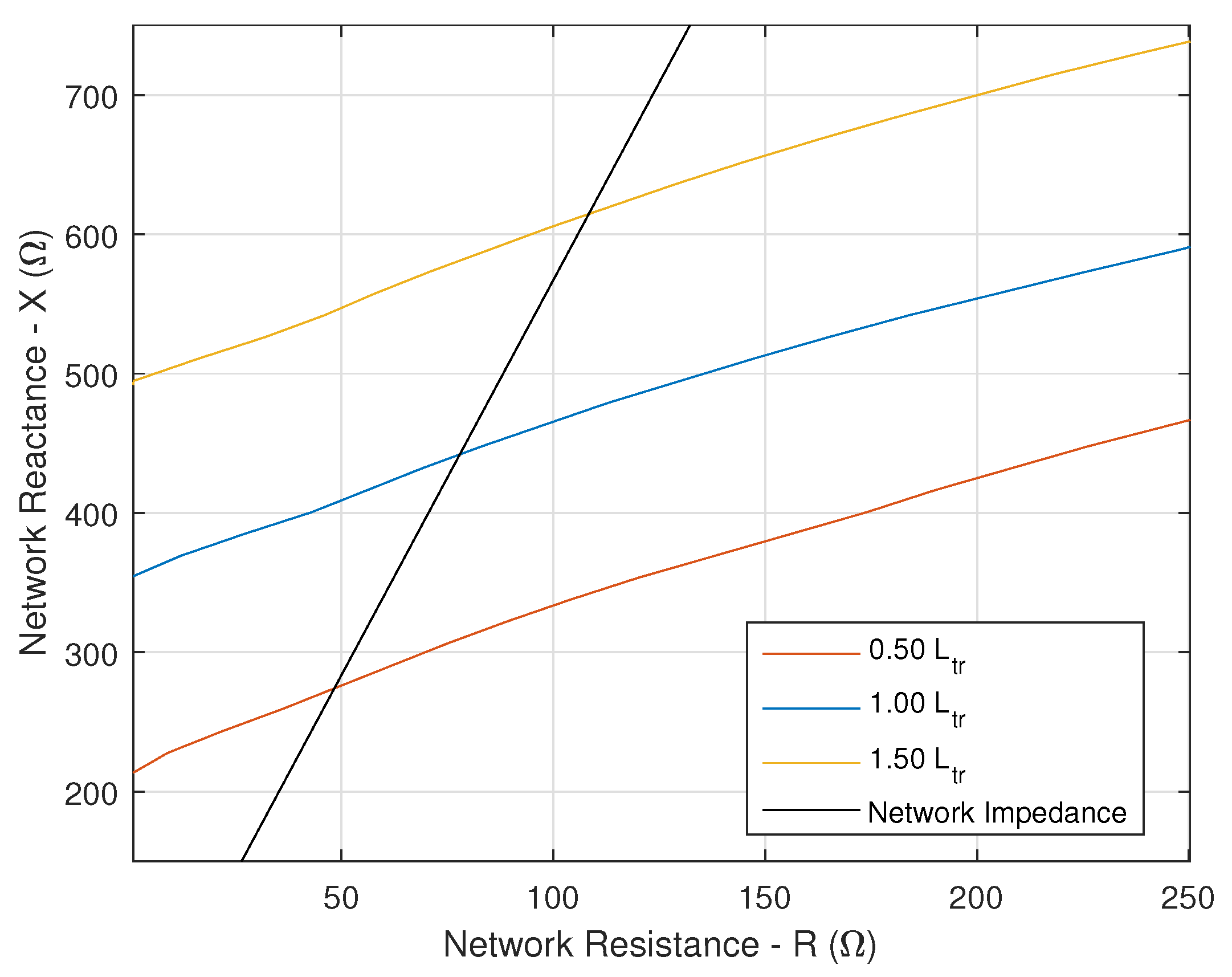
4.4. Stability Limit Curve

Figure 7 shows the stability limit curve of the traction chain in the network reactance ( X ) and resistance ( R ) complex plane with an additional dimension to show the oscillation frequency. The stability limit curve separates the stable region and unstable region.
From this figure, it can be seen that to go from the unstable region to the stable region, the network resistance must be increased, which suggests that this resistance works as a damping mechanism. On the other hand, for larger values of the reactance, the railway traction power system becomes unstable.
Two different types of contact-lines with a different ratio of reactance and resistance (i.e., different phase) are considered in this example to locate the stability limit. The contact-line impedance grows linearly with the distance (as a parametric variable) until reaching the stability limit, which is the crossing point between the SLC and the impedance linear curve. Figure 7 shows the operating point of the three study cases when the traction chain is located at a different distance from the substation.

5. Influence of Power Absorbed at the DC-Link of the Traction Chain

For this study, the case at stability limit from Section 4 is considered as a reference (i.e., base case). System stability is studied for variations in power consumption at the DC link. For this purpose, the traction chain input admittance matrix is calculated for different power levels and stability is checked using the network base impedance ( Z = Z s ) from the last section.
Since the eigenvalue λ 2 has no risk of instability, it is neither considered nor plotted. A Bode diagram of the system eigenvalue λ 1 is shown in Figure 8, where the evolution of the gain margin and the phase margin are determined as a function of power consumption from 100 kW to 1.2 MW. Increasing the power from 100 to 500 kW increases the gain and phase margin while it reduces the oscillation frequency; thus, the system stability is improved, and the limit distance increases as well. This is also seen in Figure 9, which shows the stability limit curve plotted for different levels of power. The intersection point of each stability limit curve with the network impedance gives the distance limit and the maximum network impedance that ensures stability for each power level. It is important to note that for power levels greater than 500 kW, the phase of the eigenvalue λ 1 is always below the limit 180 ° (cf. Figure 8), so the gain margin becomes infinite and there is no risk of instability at any distance for this specific contact-line. This also can be appreciated from Figure 9, where the stability limit curves for power levels of 600 kW and 700 kW never cross the network impedance curve.
Figure 9 shows that the slope of SLC increases with power, which means that at higher power consumption less damping (i.e., network resistance) is needed to maintain system stability. From this figure, the initial point of SLC at R = 0 Ω increases with power consumption in a non-linear manner.
Although it is shown that for high power levels the system stability improves and the risk of instability is eliminated, the phase diagram from Figure 8 shows that at very high powers the phase margin starts to decrease going closer to 180 ° at very low frequencies. Therefore, the risk of instability needs to be checked at very high powers as well as for low power to ensure LFO stability, as was performed in this study.
Similar behavior of low frequency stability has been reported in [4,10] for variations in power consumption. In contrast to this paper where stability analysis is performed in the frequency-domain, eigenmodes identification techniques were used in [4,10] to determine the stability limit.

6. Influence of Current Controller and 4QC Transformer’s Leakage Inductance

This section discusses the impact that the inner current controller can have on LFO formation, as well as the influence of leakage inductance of the traction chain transformer. Stability analysis is performed using the network impedance at the stability limit of the reference case ( Z = Z s ) presented in Section 4. The power consumed at the DC link is P D C = 100 kW.

6.1. Influence of Current Controller

The input admittance of a traction chain was calculated for different values of the current controller bandwidth ( ω b c c = 2 π · B W c c ), so k p c c and k i c c were modified and tuned using Equation (1), the rest of electrical and control parameter remaining constant.
According to Figure 10 and Figure 11, increasing the current controller bandwidth leads to a raise of the gain margin, which improves system stability and increases the distance limit. Moreover, it is noticed that the oscillation frequency at the stability limit (i.e., crossover frequency) increases as well.
As shown in Figure 11, the stability limit curve shifts parallel to the base case at B W c c = 100 Hz and proportionally to the variation of the bandwidth. This characteristic suggests a linear relationship between the current control bandwidth and the maximum distance from the substation that a traction chain can reach (it could also be the maximum number of traction units in the line, see Section 3.1).

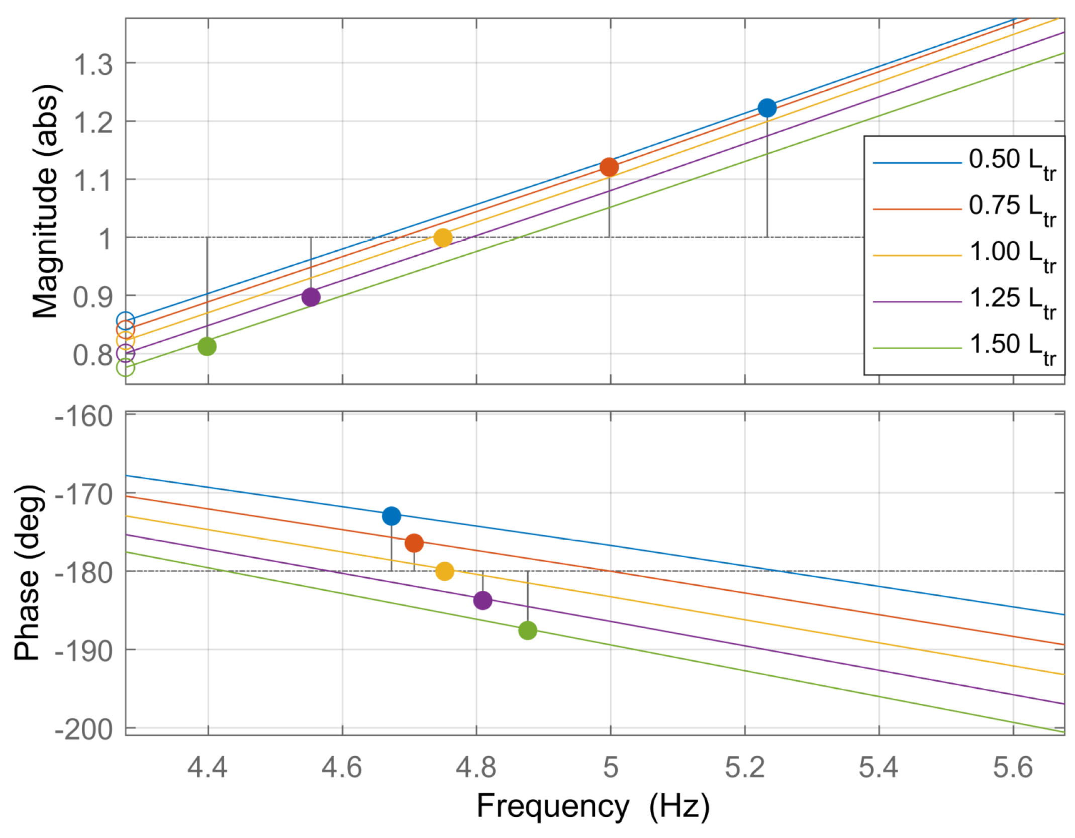
6.2. Influence of the Transformer Leakage Inductance

Figure 12 shows the Bode diagram of eigenvalue λ 1 when variations of the transformer leakage inductance L t r are performed from 50% to 150% of the nominal value (1 mH). The rest of the electrical and control parameters are kept constant. From this figure, larger values of the leakage inductance improve LFO stability, while the crossover frequency is reduced. Furthermore, Figure 13 shows that for larger values of leakage inductance, the stability limit curve shifts up parallel to the reference curve. From these figures, a linear relation seems to be present among the transformer leakage inductance, the gain margin, and the distance limit.
It is important to notice that increasing the leakage inductance, while current controller gains remain constant, results in a decrease of the bandwidth of the current control, which should decrease the stability limit according to results found in Section 6.1. Therefore, two effects are happening at the same time in this analysis, and they are opposite. The next section deals with this issue to determine the real effect of leakage inductance variations.

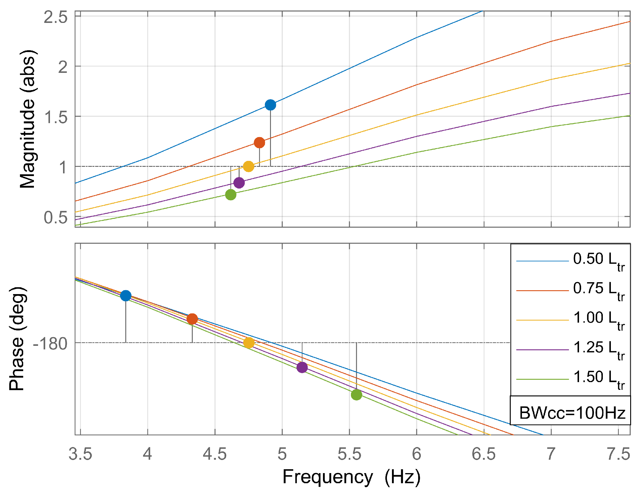
6.3. Transformer Leakage Inductance Variation with Constant Current Controller Bandwidth

In this section, variations in the leakage inductance are made while the control parameters k p c c and k i c c are re-tuned to maintain the current regulator bandwidth constant at 100 Hz. Figure 14 shows the eigenvalue λ 1 and the gain margin for different values of the inductance, from 50% to 150% of the nominal value (1 mH), as in the previous section. It can be seen that increasing L t r increases the gain margin; thus, the stability is improved. This is also confirmed by the results shown in Figure 15, where stability limit curves resulting from inductance variations are parallel to the reference case. From this figure, a linear relation between the inductance variation and the limit distance is also suggested.

6.4. Summary

Table 3 summarizes the analysis performed in this section. A linear relationship among leakage inductance, current controller bandwidth, and the gain margin was found in this study. The variation of the current controller bandwidth as described in Section 6.1 results in proportional variation of the stability margin. According to Section 6.3, when the controllers are adjusted to keep the bandwidth constant, the independent effect of the leakage inductance variation provokes proportional variations in the gain margin as well. On the other hand, from Section 6.2, it is known that the variation of only the leakage inductance implies the contrary effect on the bandwidth; therefore, a coupled effect that cancels the action of the inductance variation is presented; thus, the gain margin variation results in the superposition of the first two independent effects as shown in the table.
Comparing Figure 13 and Figure 15, it is clear that the effect of leakage inductance variations while keeping constant the current control bandwidth has a larger impact compared to the case where only leakage inductance is modified.

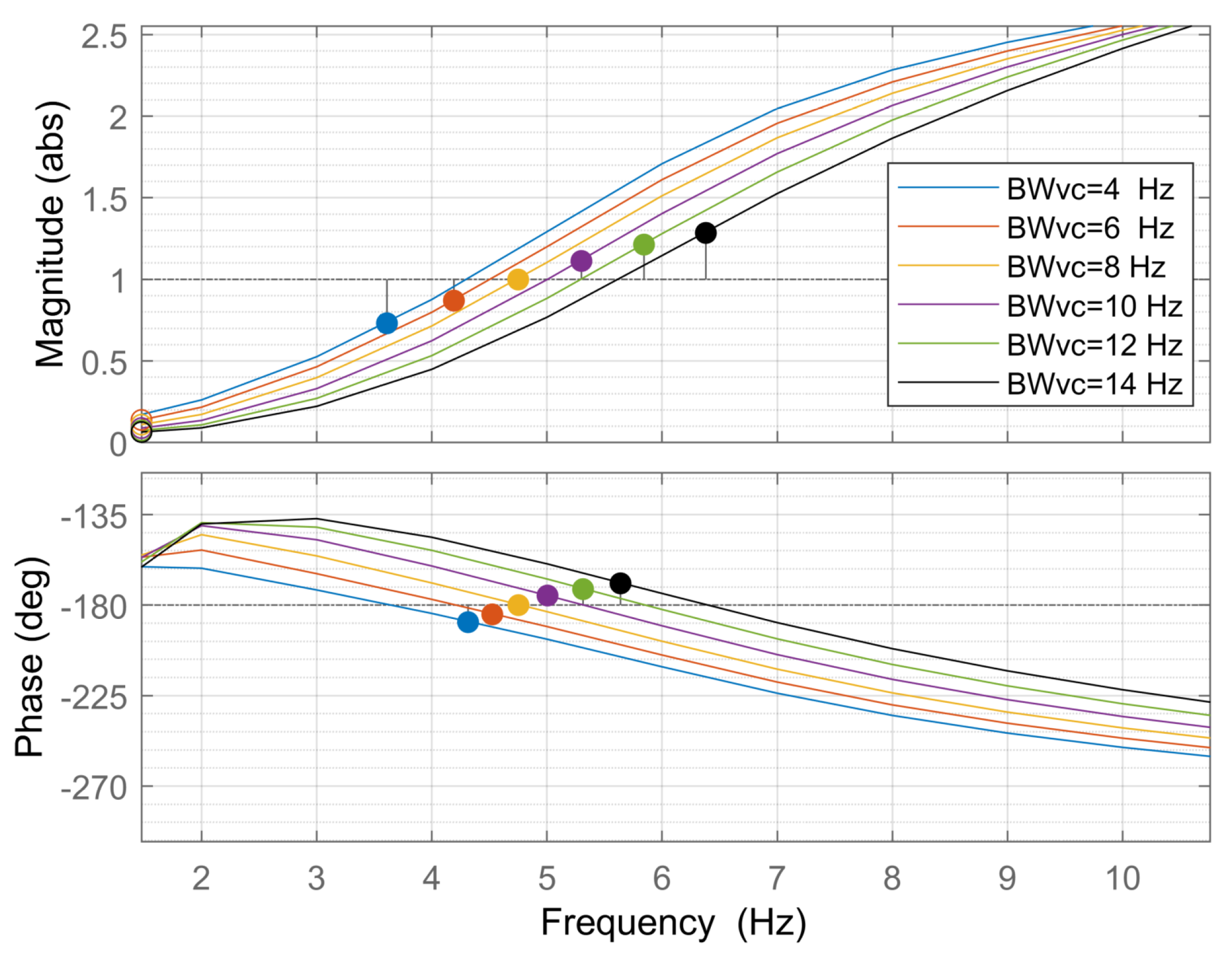
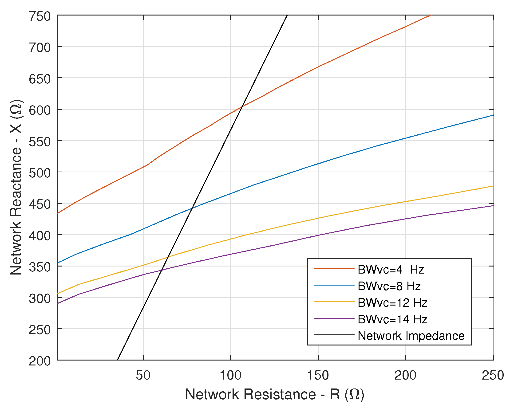
7. Influence of Voltage Controller Bandwidth and DC-Link Capacitance

This section discusses the impact that the voltage controller can have on LFO stability, as well as the influence of the DC-link capacitance. Stability analysis is performed using the network impedance at the stability limit of the reference case ( Z = Z s ) presented in Section 4. The power consumed at the DC link is P D C = 100 kW.

7.1. Influence of Voltage Controller Bandwidth

The input admittance of the traction chain was calculated for different values of the voltage controller bandwidth ( ω b v c = 2 π · B W v c ), with k p v c and k i v c being tuned using Equation (2). The remaining electrical and control parameters have been kept constant.
According to Figure 16 and Figure 17, decreasing the voltage controller bandwidth increases the gain margin, which improves system stability and increases the distance limit. Furthermore, it is observed that this action provokes the oscillation frequency decreases. From Figure 17, smaller values of voltage controller bandwidth have stability limit curves with larger slopes, which means that less damping (i.e., network resistance) is needed to maintain system stability when the network inductance increases.

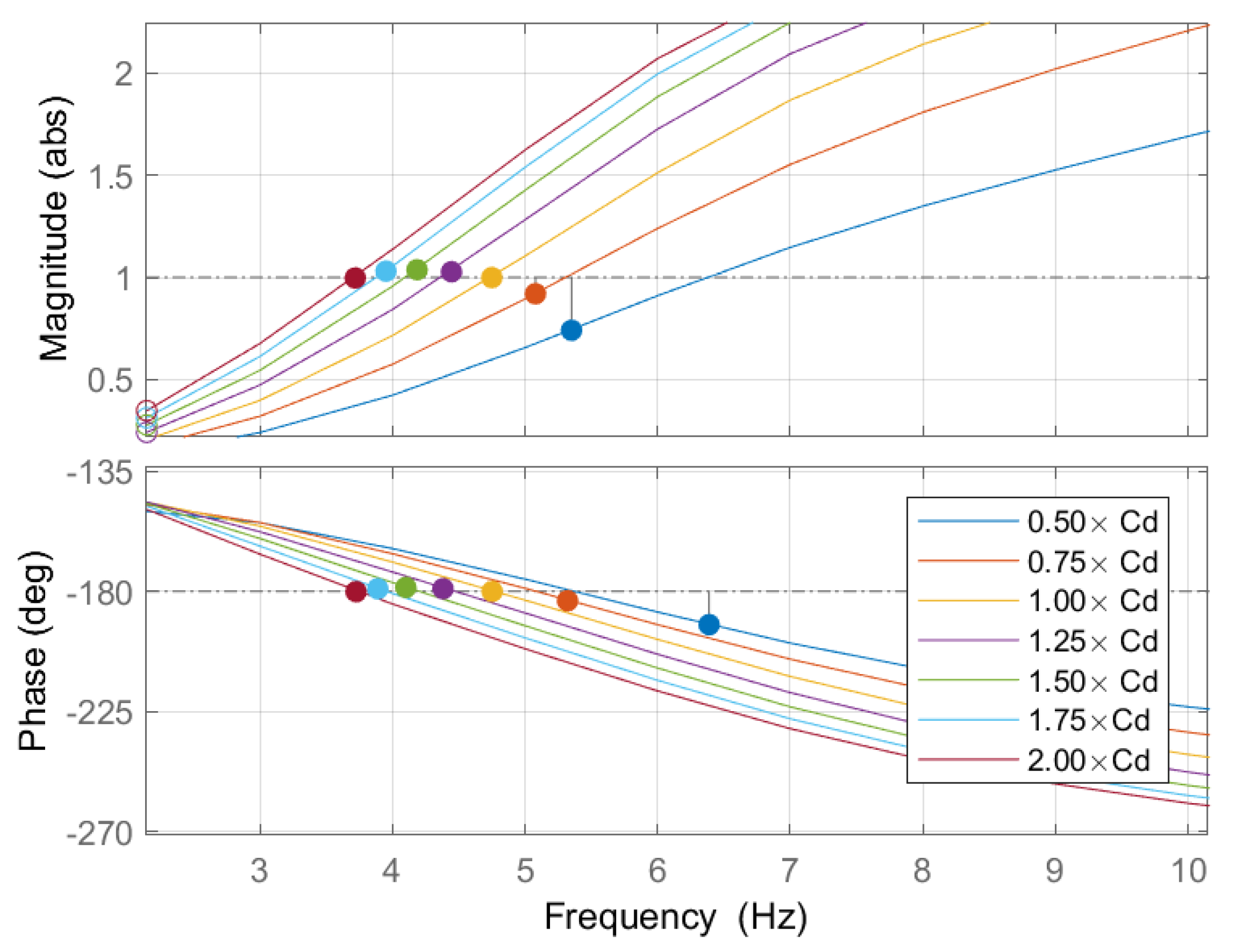
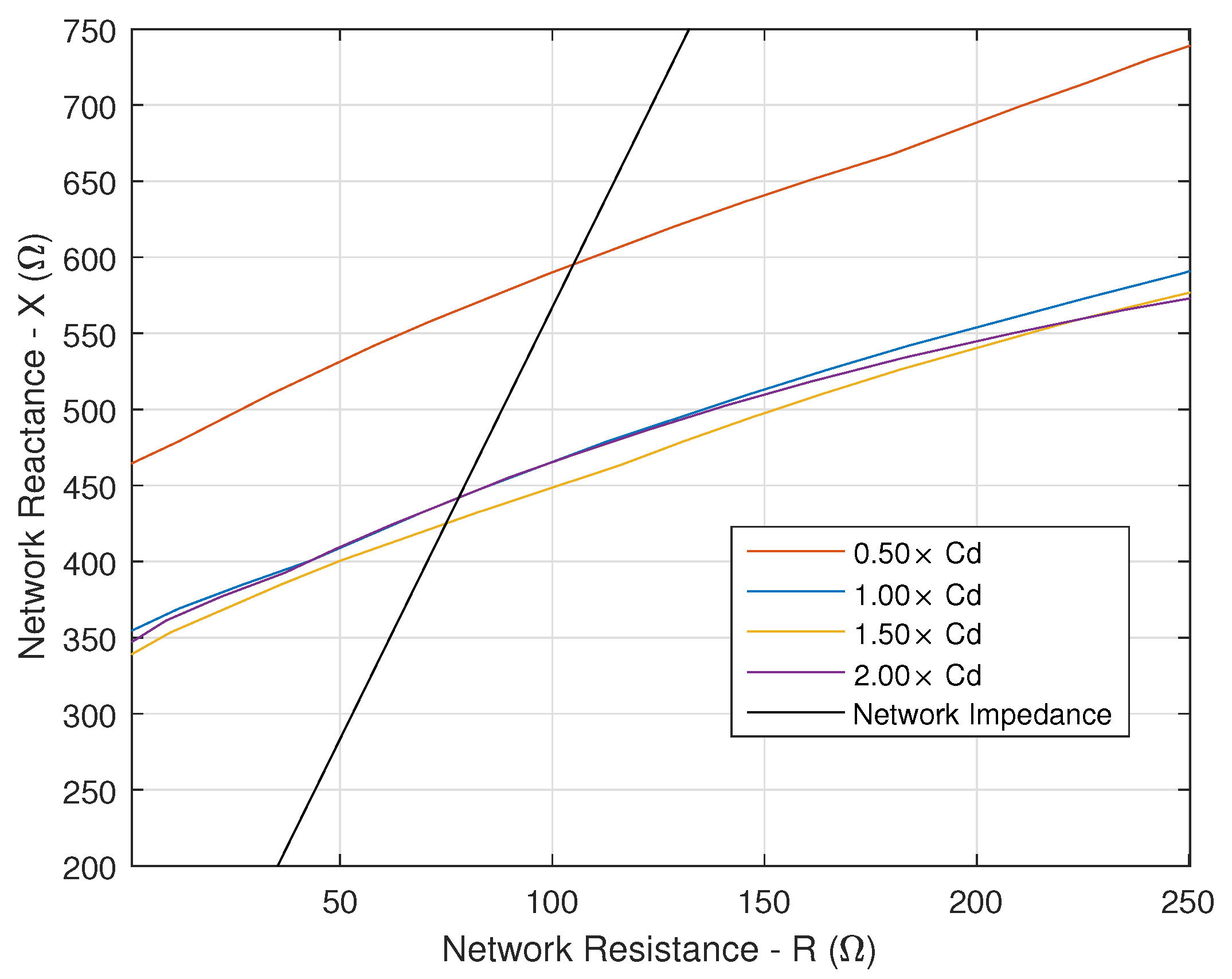
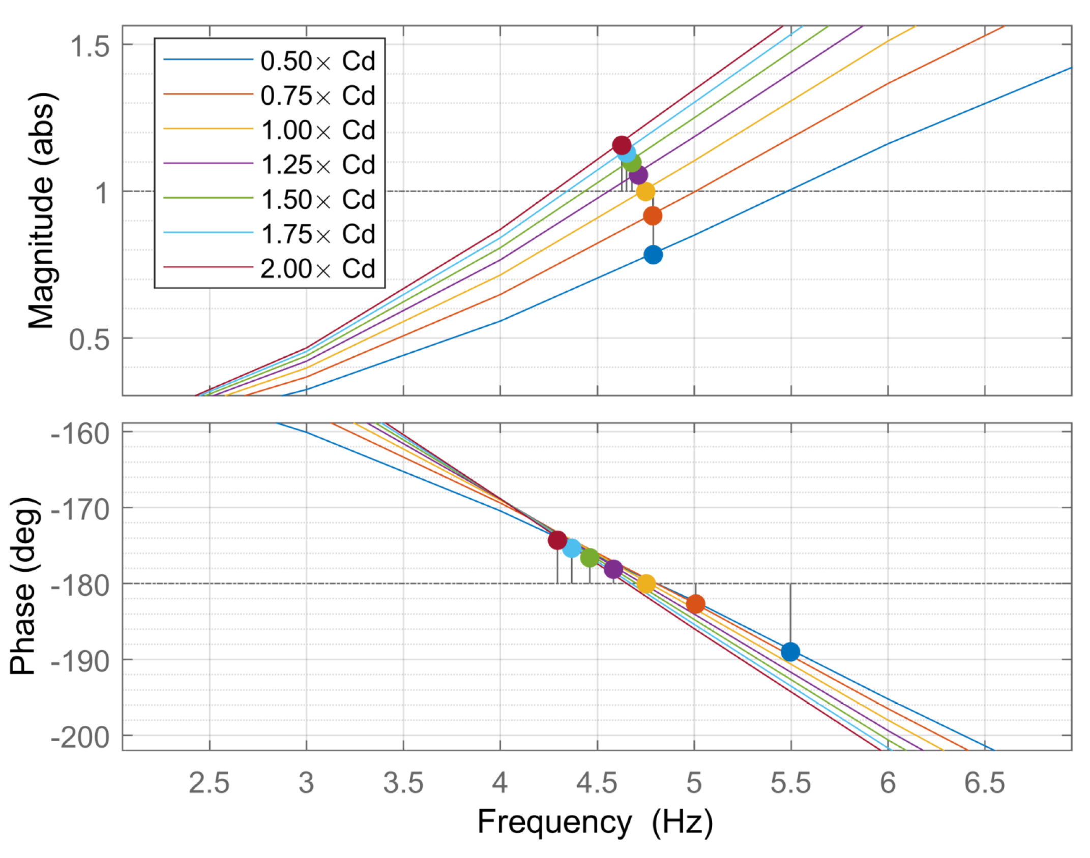
7.2. Influence of DC-Link Capacitance

Figure 18 shows the Bode diagram of the critical eigenvalue λ 1 for different values of the DC-link capacitance, from 50% to 200% of its nominal value (16 mF). Other electrical and control parameters are kept constant.
Variation of DC-link capacitance has a non-linear impact on LFO stability: decreasing C d increments the gain margin; thus, stability is improved and the crossover frequency increases. On the other hand, increasing C d leads to an unstable system, but at some point, this action is reversed, so at double the nominal value, the system becomes stable again. This behavior is also appreciated in Figure 19, which shows that decreasing capacitance by half has a considerable improvement in the stability limit curve. Increasing capacitance slightly decreases the stability limit, but when the capacitance reaches 200% of its nominal value, the limit is the same as the reference case.
It is important to note that the variation in DC-link capacitance implies that the voltage controller bandwidth is modified as well, so the next section analyzes this issue.

7.3. DC-Link Capacitance Variation with Constant Voltage Controller Bandwidth

In this section, variations in the DC-link capacitance are made while the control parameters k p v c and k i v c are tuned in order to maintain a constant bandwidth of 8 Hz according to Equation (2).
Figure 20 shows the eigenvalue λ 1 and the gain margin evolution for different values of the capacitance, from 50% to 200% of its nominal value (16 mF). Decreasing C d from the nominal value raises the gain margin; thus, stability is improved. On the other hand, increasing C d leads to an unstable system.
Figure 21 shows that decreasing capacitance moves the stability limit curve up, and increasing the capacitor takes the curve down. From these two figures, the non-linear relationship between the variations of DC-link capacitance, gain margin and stability limit is appreciated, since the sensitivity of the variation is not the same. Gain margin and stability limit variations seem to be more sensitive at lower values of C d .

7.4. Discussion

Although the study for the variation of voltage controller bandwidth and DC-link capacitance shows a non-linear relationship among these parameters and the stability margins, lower voltage control loop bandwidths and lower values of DC-link capacitance always improve the LFO stability in the range of variations performed in this study.
A linear behavior was found only in a very small variation range (around 10% of nominal values). Table 4 summarizes the relationships between the variation of the parameters and the stability margins for very small variations.
From Table 4, three linear events are identified. First, decreasing the voltage controller bandwidth increases stability margins. Second, variation of DC-link capacitance, while the voltage controller bandwidth is kept constant, is inversely proportional to the variation of the stability margin. Finally, decreasing only the DC-link capacitance implies the superposition of the first two events. These trends can be seen in Figure 22, which shows that decreasing capacitance by 10% while BWvc is kept constant (i.e., re-tuning controllers) goes further to the right of the critical point (i.e., more stable) than the case when only the capacitance is decreased.

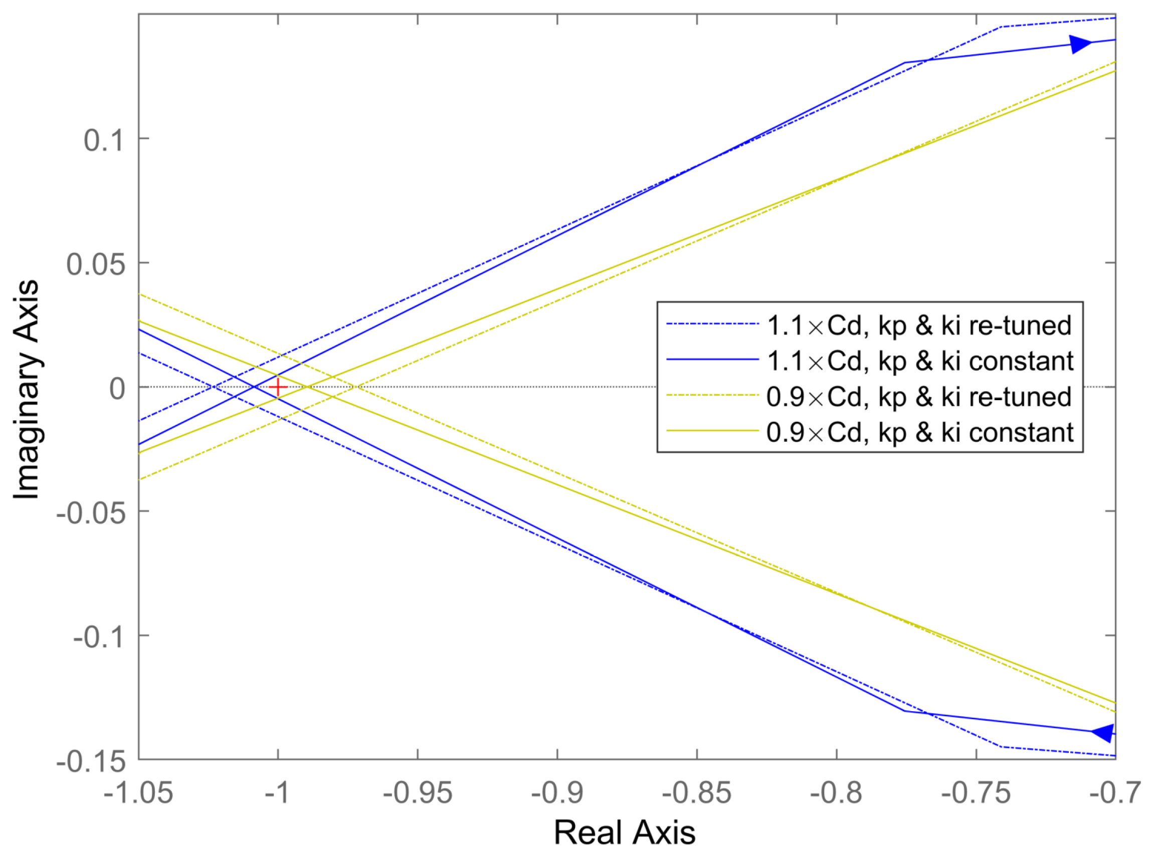
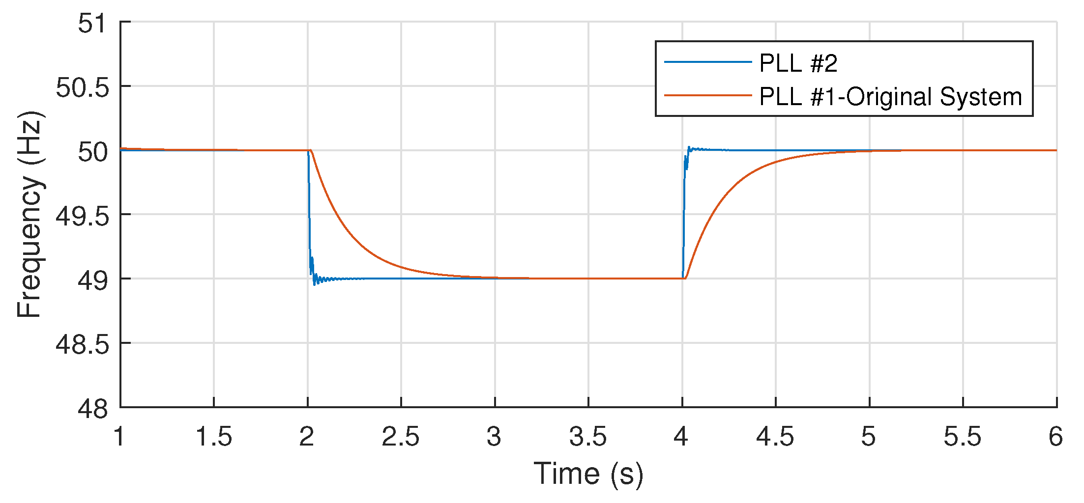
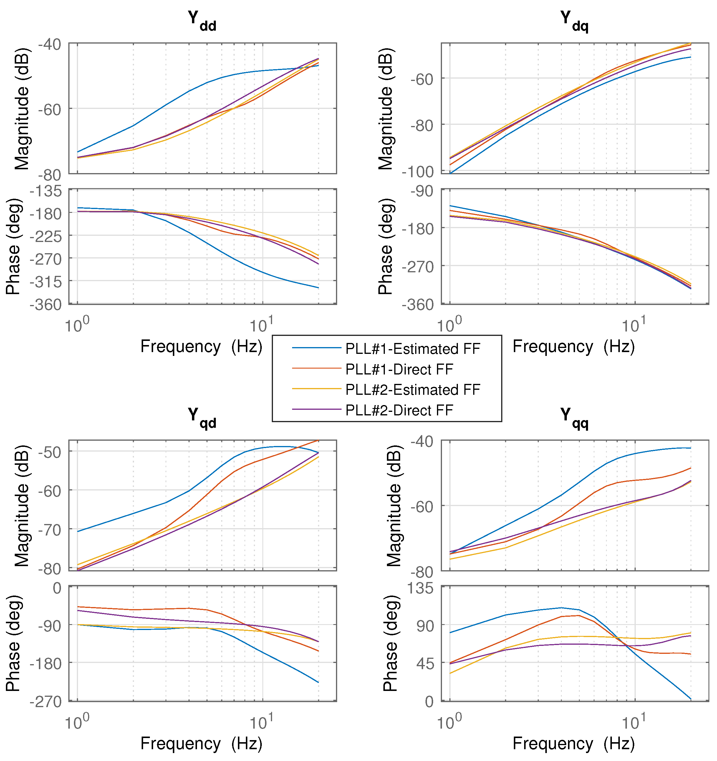
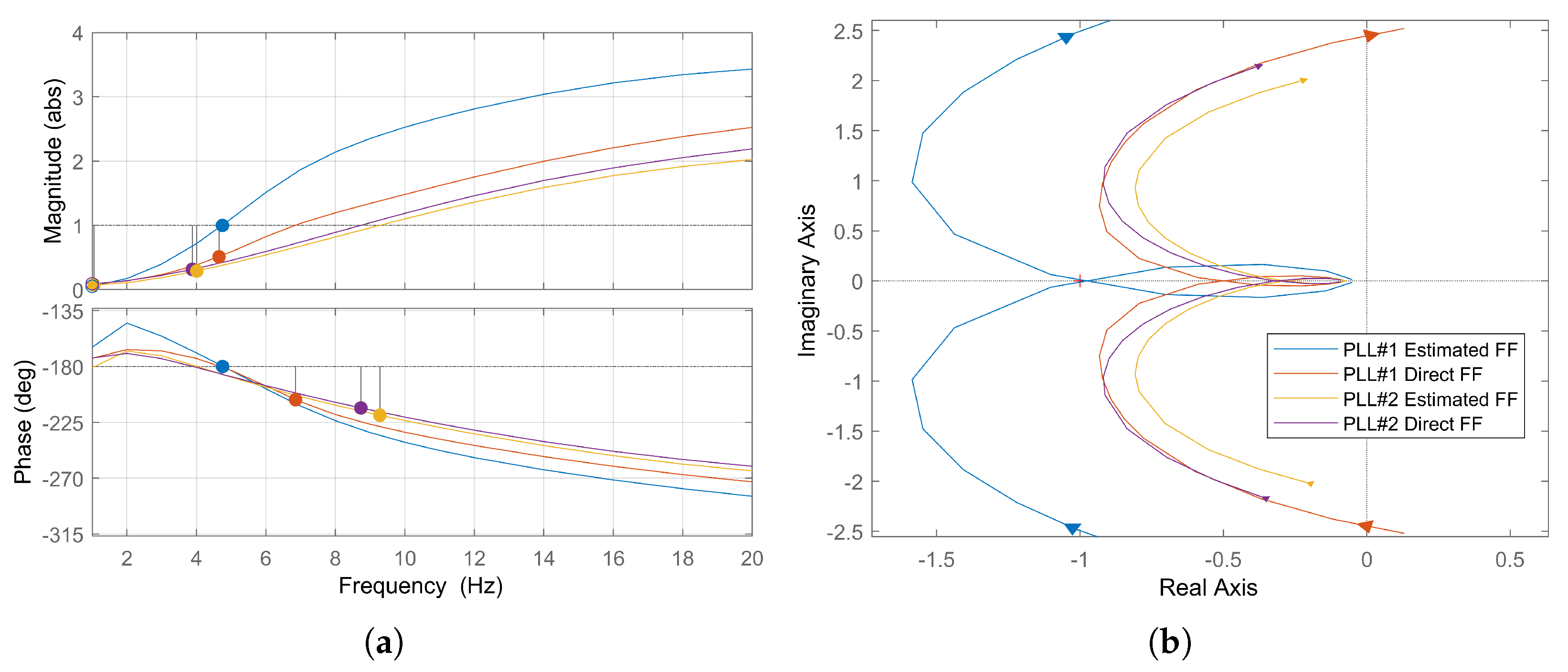
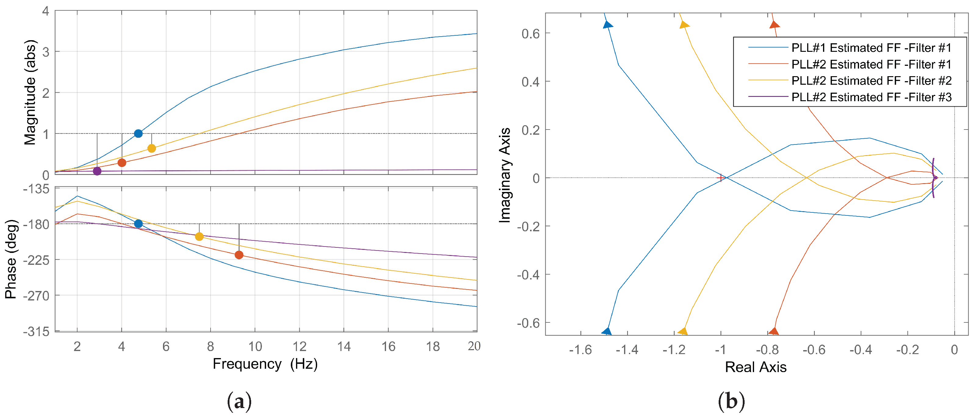
8. Impact of Phase-Locked Loop and Feedforward Signal

In this section, the influence of the PLL and the feedforward signal are studied. Two PLL options are considered: PLL #1 is the synchronization method described in [13], which achieves the synchronization by determining the zero-crossing of contact-line voltage. PLL #2 is described in [22] and it consists of a phase detector in a feedback loop; this option uses an adaptive second-order generalized integrator (SOGI) to generate the quadrature signal.
Figure 23 shows the estimated frequency time response for both cases when a step occurs in the frequency of the contact-line voltage. Both systems are able to track the frequency changes, with the only difference being that PLL #2 is faster than the original synchronization system.
With both PLL systems, two different configurations are considered for the generation of the feedforward signal V f f shown in the control diagram in Figure 2c. In addition to the use of the feedforward estimator block, the signal V f f can also be generated directly from the output of the contact-line voltage filter as shown in [4]; thus, V f f = V r f . Therefore, four different cases are studied and compared, which is summarized in Table 5. Figure 24 shows the traction chain input admittance, and Figure 25 shows the critical system eigenvalue λ 1 using Bode and Nyquist plots for the four study cases.
Case 1 is the reference case, using the original synchronization system PLL #1 and the feedforward estimator. According to Figure 25, the original case is at the stability limit ( G M = 1 ). The replacement of only the PLL (i.e., case 2) improves the stability margin by a factor larger than 2. With case 3, only the generation of the feedforward signal is modified, and the stability is improved by at least a factor of 2. In summary, replacing only the PLL or only the feedforward estimator improves stability. In case 4, both the PLL and feedforward are modified; as expected, system stability improves, but the improvement is not the addition of each individual effect of cases 2 and 3.
The stability analysis of cases 1 and 2 might suggest that PLL #1 is the main source of instabilities. However, the large stability margin of case 3 would not support this assumption. For cases 3 and 4, the feedforward signal is taken directly from the voltage filter, which means that no dynamic influence of the synchronization system exists in the generation of the feedforward signal. Thus, the impact of the PLL can only be noticed when the estimator block is used to generate the feedforward signal such as in cases 1 and 2. Since the main difference between PLL #1 and PLL #2 is the system delay in the transient state as shown in Figure 23, this suggests that the delay in the feedforward signal has an important influence on LFO stability.
In summary, large stability margins are presented in cases 3 and 4 since only the small delay of the contact-line voltage filter influences the feedforward signal dynamics. A fast synchronization system, such as PLL #2 in case 2, results in a small delay of the feedforward signal as well. On the other hand, in case 1, the low dynamics by the synchronization system results in a large feedforward delay.
To check this hypothesis (i.e., the influence of the feedforward signal delay), the original (Filter #1) contact-line voltage filter, from Figure 2c, in charge of filtering the third and fifth voltage harmonics, was first replaced by a band-pass filter (Filter #2) with a slower dynamic and later by a first-order high bandwidth low pass filter (Filter #3) that has a very fast dynamic. It is important to mention that the goal of this study was not the rejection of harmonics, but rather a sinusoidal contact-line voltage waveform with no harmonics is considered; therefore, the criterion for choosing the voltage filter was based on the speed of the dynamic response that minimizes delays. Filter #3 is closer to the case of having no filter since almost no delays are present.
Figure 26 shows the traction chain input admittance, and Figure 27 shows the critical system eigenvalue λ 1 using Bode and Nyquist plots for the three different filters; PLL #2 and the estimated feedforward signal are used for this analysis, and the original reference case is also plotted. As the hypothesis suggested, the stability margin is proportional to the filter delay, and from the figure is clear that the system with the fastest filter (i.e., Filter #3) has the largest gain margin.
Figure 26 shows that for the cases with better stability margins, the phase of the input admittance Y q q gets closer to 0 ° at very low frequencies (i.e., the gain margin is proportional to the phase of the input admittance Y q q at very low frequencies).

9. Conclusions

In this paper, impedance-based stability analysis techniques in the frequency-domain have been used to study the impact of electrical and control parameters in the appearance of low frequency oscillations, including contact-line length (i.e., distance from substation), consumed power, bandwidth of current and voltage controllers, leakage inductance of transformer, DC-link capacitor, synchronization system and feedforward signal. Time-domain simulations were further used to validate the results of the analysis.
The influence of the contact-line length and number of traction chains on LFO has been widely reported. The study of the impact of power consumption shows that the worst case for instability is at low power. The stability limit curve for different power consumption levels was presented with a specific pattern of its evolution.
It has been concluded that current control bandwidth and stability margins have a linear relationship. Variations of transformer leakage inductance are inversely proportional to the current control bandwidth, this effect can be canceled by tuning controllers to keep the bandwidth constant; then, the leakage inductance and stability margins will also show a linear relationship.
Decreasing voltage controller bandwidth increases gain margin. On the other hand, the variation of DC-link capacitance showed a non-linear relationship with the stability margins, where increasing capacitance decreases stability margins and voltage controller bandwidth, but at some point, stability margins will be reversed. Finally, decreasing DC-link capacitance while keeping constant the voltage controller bandwidth causes a monotonous improvement of the system stability for the range of variations considered in this study.
Faster dynamics for the PLL improves the low-frequency stability. Delays of the feedforward signal were observed to increase the risks of LFO, but this topic requires further research.
For future research on low-frequency stability, the influence of using different types of compensators for the control of the onboard transformer current should be studied. Proportional resonant compensators and PI compensators in the dq reference frame should be considered; therefore, a comparative analysis can be performed. As already mentioned, the low-frequency stability for multiple trains located at different positions of the contact-line was out of the scope of this paper but it should be considered for future research since it has not been reported yet.

Author Contributions

Methodology, P.L. and N.R.; traction chain model, P.L. and N.R.; implementation of scanning algorithms P.F.; software and simulations, P.F.; analysis P.F.; validation, P.L., N.R. and F.B.; writing—original draft preparation, P.F.; writing—review and editing, P.F., P.L., N.R., F.B., J.M.G. and I.L. All authors have read and agreed to the published version of the manuscript.

Funding

This research was partially funded by the Government of Asturias under grant AYUD/2021/50988 and FEDER funds.

Institutional Review Board Statement

Not applicable.

Informed Consent Statement

Not applicable.

Data Availability Statement

The data presented in this study are available upon request from the corresponding author.

Conflicts of Interest

The authors declare no conflict of interest.

References

  1. Danielsen, S.; Molinas, M.; Toftevaag, T.; Fosso, O. Constant power load characteristic’s influence on the low-frequency interaction between advanced electrical rail vehicle and railway traction power supply with rotary converters. In Proceedings of the MET’ 2009, Gdanjsk, Poland, 24–26 September 2009. [Google Scholar]
  2. Buhrkall, L.; Danielsen, S.; Eisele, A.; Bergman, M.; Galic, J. Low-frequency oscillations in Scandinavian railway power supply—Part I: Basic considerations. eb-Elektr. Bahnen 2010, 108, 56–64. [Google Scholar]
  3. Buhrkall, L.; Danielsen, S.; Eisele, A.; Bergman, M.; Galic, J. Low-frequency oscillations in Scandinavian railway power supply—Part 2: Test of traction units. eb-Elektr. Bahnen 2010, 108, 103–111. [Google Scholar]
  4. Danielsen, S. Electric Traction Power System Stability: Low-Frequency Interaction between Advanced Rail Vehicles and a Rotary Frequency Converter. Ph.D. Thesis, Norwegian University of Science and Technology, Trondheim, Norway, April 2010. [Google Scholar]
  5. Suarez, J.; Ladoux, P.; Roux, N.; Caron, H.; Guillame, E. Measurement of locomotive input admittance to analyse low frequency instability on AC rail networks. In Proceedings of the 2014 International Symposium on Power Electronics, Electrical Drives, Automation and Motion, Ischia, Italy, 18–20 June 2014; pp. 790–795. [Google Scholar] [CrossRef]
  6. Menth, S.; Meyer, M. Low frequency power oscillations in electric railway systems. eb-Elektr. Bahnen 2006, 104, 216–221. [Google Scholar]
  7. Wang, H.; Mingli, W.; Sun, J. Analysis of Low-Frequency Oscillation in Electric Railways Based on Small-Signal Modeling of Vehicle-Grid System in dq Frame. IEEE Trans. Power Electron. 2015, 30, 5318–5330. [Google Scholar] [CrossRef]
  8. Hu, H.; Tao, H.; Blaabjerg, F.; Wang, X.; He, Z.; Gao, S. Train–Network Interactions and Stability Evaluation in High-Speed Railways–Part I: Phenomena and Modeling. IEEE Trans. Power Electron. 2018, 33, 4627–4642. [Google Scholar] [CrossRef]
  9. Hu, H.; Tao, H.; Wang, X.; Blaabjerg, F.; He, Z.; Gao, S. Train–Network Interactions and Stability Evaluation in High-Speed Railways—Part II: Influential Factors and Verifications. IEEE Trans. Power Electron. 2018, 33, 4643–4659. [Google Scholar] [CrossRef]
  10. Frutos, P.; Guerrero, J.M.; Muniategui, I.; Vicente, I.; Endemano, A.; Briz, F. Low-Frequency Oscillations Analysis in AC Railway Networks Using Eigenmode Identification. In Proceedings of the 2021 IEEE Energy Conversion Congress and Exposition (ECCE), Vancouver, BC, Canada, 10–14 October 2021; pp. 1573–1579. [Google Scholar] [CrossRef]
  11. Hachicha, Y.; Cypers, D.; Takuefou, M.; Belin, S.; Ladoux, P.; Roux, N. Use of a HIL railway traction simulator for low frequency network stability studies. In Proceedings of the 2018 IEEE International Conference on Electrical Systems for Aircraft, Railway, Ship Propulsion and Road Vehicles International Transportation Electrification Conference (ESARS-ITEC), Nottingham, UK, 7–9 November 2018; pp. 1–5. [Google Scholar] [CrossRef]
  12. Ladoux, P.; Hachicha, Y.; Cypers, D.; Meli, M.; Roux, N. New method for determining the low-frequency Stability Limit of a 50 Hz electric traction power system. Elektr. Bahnen 2020, 18, hal-03286350. [Google Scholar]
  13. Suarez, J. Étude et Modélisation des Interactions éLectriques entre les Engins et les Installations Fixes de Traction éLectrique 25 kV/50 Hz. Ph.D. Thesis, University of Toulouse, Toulouse, France, 2014. [Google Scholar]
  14. Liao, Y.; Liu, Z.; Zhang, H.; Wen, B. Low-Frequency Stability Analysis of Single-Phase System with dq-Frame Impedance Approach—Part I: Impedance Modeling and Verification. IEEE Trans. Ind. Appl. 2018, 54, 4999–5011. [Google Scholar] [CrossRef]
  15. Hachicha, Y.; Cypers, D.; Belin, S.; Meli, M.; Ladoux, P.; Roux, N. Towards a unified low frequency Stability criterion for 15 kV/16.7 Hz and 25 kV/50 Hz railway power system. In Proceedings of the PCIM Europe Digital Days 2020; International Exhibition and Conference for Power Electronics, Intelligent Motion, Renewable Energy and Energy Management, Virtual, 7–8 July 2020; pp. 1–8. [Google Scholar]
  16. Buhrkall, L. Traction system case study. In Proceedings of the 2008 IET Professional Development course on Electric Traction Systems, Manchester, UK, 3–7 November 2008; pp. 45–63. [Google Scholar] [CrossRef] [Green Version]
  17. EN 50388-2:2017. Railway Applications—Fixed Installations and Rolling Stock—Technical Criteria for the Coordination between Power Supply and Rolling Stock to Achieve Interoperability—Part 2: Stability and Harmonics. Available online: https://standards.iteh.ai/catalog/standards/clc/f5fb00d6-1f29-4dd4-a8fd-e3e478907499/pren-50388-2-2017 (accessed on 7 July 2017).
  18. Ogata, K. Modern Control Engineering (Instrumentation and Controls Series); Prentice-Hall, Inc.: Upper Saddle River, NJ, USA, 2010. [Google Scholar]
  19. Liao, Y.; Liu, Z.; Zhang, H.; Wen, B. Low-Frequency Stability Analysis of Single-Phase System With dq-Frame Impedance Approach—Part II: Stability and Frequency Analysis. IEEE Trans. Ind. Appl. 2018, 54, 5012–5024. [Google Scholar] [CrossRef]
  20. Pendharkar, I. A generalized Input Admittance Criterion for resonance stability in electrical railway networks. In Proceedings of the 2014 European Control Conference (ECC), Strasbourg, France, 24–27 June 2014; pp. 690–695. [Google Scholar] [CrossRef]
  21. Wang, X.; Blaabjerg, F. Harmonic Stability in Power Electronic-Based Power Systems: Concept, Modeling, and Analysis. IEEE Trans. Smart Grid 2019, 10, 2858–2870. [Google Scholar] [CrossRef] [Green Version]
  22. Teodorescu, R.; Liserre, M.; Rodriguez, P. Grid Synchronization in Single Phase Power Converters. In Grid Converters for Photovoltaic and Wind Power Systems; John Wiley & Sons: West Sussex, UK, 2011; pp. 43–91. [Google Scholar] [CrossRef]
Figure 1. Contact-line voltage and current supplied by the substation. AC 25 kV/50 Hz electric power supply. Measured in Thionville, France. Reprinted with permission from Ref. [5]. Copyright 2014 IEEE.
Electronics 11 01593 g001
Figure 2. Railway system model and control. (a) Railway traction power system, (b) Simplified railway system model for the study of LFO. (c) Traction chain control system.
Electronics 11 01593 g002
Figure 3. Closed loop system equivalence of small-signal model for n network impedance units and m traction chains. (a) Railway traction system small-signal model, (b) closed loop system.
Electronics 11 01593 g003
Figure 4. Traction-chain input admittance. Frequency range: 1–20 Hz.
Electronics 11 01593 g004
Figure 5. System eigenvalues ( λ 1 , λ 2 ) of the three study cases. Stable case (red): gain margin = 2 at 4.75 Hz; stability limit case (blue): gain margin = 1 at 4.75 Hz; unstable case (yellow): gain margin = 0.667 at 4.75 Hz. (a) Bode Diagram, (b) Nyquist Diagram.
Electronics 11 01593 g005
Figure 6. Time-domain simulations. From top to bottom: DC-link voltage, contact-line voltage and train current. Step changes of power supply impedance are consecutively applied along the simulation time. The stable case, stability limit case and unstable case are found at times t = 5 s, t = 6 s and t = 8 s, respectively.
Electronics 11 01593 g006
Figure 7. Stability limit curve of the traction chain in the network reactance ( X ) and resistance ( R ) complex plane with the corresponding oscillation frequencies. At P D C = 100 kW. Power supply system: 25 kV/50 Hz.
Electronics 11 01593 g007
Figure 8. Bode diagram of system eigenvalue λ 1 for different levels of power consumption. Network Impedance: Z = Z s .
Electronics 11 01593 g008
Figure 9. Stability limit curve of traction chain in the network reactance ( X ) and resistant ( R ) complex plane. Different levels of power consumption.
Electronics 11 01593 g009
Figure 10. Bode diagram of the system eigenvalue λ 1 . Variation of current controller bandwidth.
Electronics 11 01593 g010
Figure 11. Stability limit curve of a traction chain in the network reactance ( X ) and resistant ( R ) complex plane. Variation of current controller bandwidth.
Electronics 11 01593 g011
Figure 12. Bode diagram of the system eigenvalue λ 1 . Variation of leakage inductance.
Electronics 11 01593 g012
Figure 13. Stability limit curve of a traction chain in the network reactance ( X ) and resistance ( R ) complex plane. Variation of leakage inductance.
Electronics 11 01593 g013
Figure 14. Bode diagram of the system eigenvalue λ 1 . Variation of leakage inductance while the keeping current controller bandwidth at 100 Hz.
Electronics 11 01593 g014
Figure 15. Stability limit curve of a traction chain in the network reactance ( X ) and resistant ( R ) complex plane. Variation of leakage inductance while keeping the current controller bandwidth at 100 Hz.
Electronics 11 01593 g015
Figure 16. Bode diagram of the system eigenvalue λ 1 for different values of voltage controller bandwidth.
Electronics 11 01593 g016
Figure 17. Stability limit curve of a traction chain in the network reactance ( X ) and resistant ( R ) complex plane. Variation of voltage controller bandwidth.
Electronics 11 01593 g017
Figure 18. Bode diagram of the system eigenvalue λ 1 . Variation of DC-link capacitance.
Electronics 11 01593 g018
Figure 19. Stability limit curve of a traction chain in the network reactance ( X ) and resistant ( R ) complex plane. Variation of DC-link capacitance.
Electronics 11 01593 g019
Figure 20. Bode diagram of the system eigenvalue λ 1 . Variation of DC-link capacitance while keeping the voltage controller bandwidth at 8 Hz.
Electronics 11 01593 g020
Figure 21. Stability limit curve of a traction chain in the network reactance ( X ) and resistant ( R ) complex plane. Variation of DC-link capacitance while keeping the voltage controller bandwidth at 8 Hz.
Electronics 11 01593 g021
Figure 22. Nyquist plot for the eigenvalue λ 1 . Small variation of DC-link capacitance.
Electronics 11 01593 g022
Figure 23. Estimated frequency step response of two different phase-locked loops. The frequency of contact-line voltage is changing to f = 49 Hz at t = 2 s, and going back to f = 50 Hz at t = 4 s.
Electronics 11 01593 g023
Figure 24. Traction chain input admittance. Frequency range: 1–20 Hz. Influence of the PLL and the feedforward.
Electronics 11 01593 g024
Figure 25. System eigenvalue λ 1 . Influence of the PLL and the feedforward. (a) Bode diagram, (b) Nyquist diagram.
Electronics 11 01593 g025
Figure 26. Traction chain input admittance. Frequency range: 1–20 Hz. Contact-line voltage filter influence.
Electronics 11 01593 g026
Figure 27. System eigenvalue λ 1 . Influence of contact-line voltage filter. (a) Bode diagram, (b) Nyquist diagram.
Electronics 11 01593 g027
Table 1. LFO reported cases.
Case f 0  (Hz) f osc  (Hz)Time (Year)
1Zürich, Switzerland [1]16.751995
2Norway [2,3]16.71.62007
3Washington, USA [4]2532006
4Thionville, France [5]5052008
5Siemens test, Germany [6]5072006
6Hudong Depot, China [7]502–42008
7Shanhaiguan Hub, China [8]506–72011
Table 2. Traction chain parameters.
SymbolDescriptionValue
UContact-line voltage25 kV
f 0 Fundamental frequency50 Hz
L t r Leakage inductance1 mH
C d DC-link capacitor16 mF
B W v c Voltage control bandwidth8 Hz
B W c c Current control bandwidth100 Hz
P D C Power at DC-link100 kW
Table 3. Impact of current controller and transformer leakage inductance in LFO stability. Arrows ↑ stands for increments and ↓ stands for decrements.
L tr kp cc & ki cc AdjustedBWccStability Margins
-YES↑ ↑
YES-↑ ↑ ↑
NO↑ ↑ ↑  +  ↓↓  =  ↑
Table 4. Impact of very small variations of voltage controller and DC-link capacitance on LFO stability. Arrows ↑ stands for increments and ↓ stands for decrements.
C d kp vc & ki vc AdjustedBWvcStability Margins
-YES↑↑
YES-↑↑↑
NO↑↑↑  +  ↓↓  =  ↑
Table 5. Study cases: influence of the PLL and the feedforward (FF).
PLL #1PLL #2Estimated FFDirect FFStability Ranking
Case 1X X BAD
Case 2 XX GOOD
Case 3X XGOOD
Case 4 X XGOOD
Publisher’s Note: MDPI stays neutral with regard to jurisdictional claims in published maps and institutional affiliations.

