Smart Home Battery for the Multi-Objective Power Scheduling Problem in a Smart Home Using Grey Wolf Optimizer

Abstract

The power scheduling problem in a smart home (PSPSH) refers to the timely scheduling operations of smart home appliances under a set of restrictions and a dynamic pricing scheme(s) produced by a power supplier company (PSC). The primary objectives of PSPSH are: (I) minimizing the cost of the power consumed by home appliances, which refers to electricity bills, (II) balance the power consumed during a time horizon, particularly at peak periods, which is known as the peak-to-average ratio, and (III) maximizing the satisfaction level of users. Several approaches have been proposed to address PSPSH optimally, including optimization and non-optimization based approaches. However, the set of restrictions inhibit the approach used to obtain the optimal solutions. In this paper, a new formulation for smart home battery (SHB) is proposed for PSPSH that reduces the effect of restrictions in obtaining the optimal/near-optimal solutions. SHB can enhance the scheduling of smart home appliances by storing power at unsuitable periods and use the stored power at suitable periods for PSPSH objectives. PSPSH is formulated as a multi-objective optimization problem to achieve all objectives simultaneously. A robust swarm-based optimization algorithm inspired by the grey wolf lifestyle called grey wolf optimizer (GWO) is adapted to address PSPSH. GWO has powerful operations managed by its dynamic parameters that maintain exploration and exploitation behavior in search space. Seven scenarios of power consumption and dynamic pricing schemes are considered in the simulation results to evaluate the proposed multi-objective PSPSH using SHB (BMO-PSPSH) approach. The proposed BMO-PSPSH approach’s performance is compared with that of other 17 state-of-the-art algorithms using their recommended datasets and four algorithms using the proposed datasets. The proposed BMO-PSPSH approach exhibits and yields better performance than the other compared algorithms in almost all scenarios.

1. Introduction

Old power grids are encountering several difficulties in reducing the power demand of users, particularly in peak periods, where they cannot face the increment in power demand because of the primitive nature of their infrastructures. Accordingly, the old power grids’ stability and safety became not guaranteed. Therefore, the smart grid (SG) has emerged instead of the old power grid to face its difficulties and meet the users’ requirement of power [1].

SG upgrades and improves the old power grid’s management, control, and distribution systems. The SG communication system is playing the primary key to this improvement, where it is considered the backbone of SG. The communication system allows power supplier companies (PSCs) to transfer power to the users and get their feedback [2].

SG’s primary goals are to make power usage more efficient, diminish users’ demand for power during peak periods, and optimize the cost of power production [3]. Optimizing users’ power demand plays the leading role in attaining SG goals and making its power system more efficient [4,5]. Furthermore, this kind of optimization provides benefits for users, such as reducing electricity bill (EB) and improving their comfort level. However, the power demand of users can be optimized by scheduling the operations of appliances in a smart home or Internet-of-Things at suitable periods in accordance with a dynamic price scheme(s) (i.e., the electricity prices vary dynamically over time) [6,7,8,9,10].

PSCs generate dynamic pricing schemes on the basis of the cost of power generation and power demand, where electricity prices are high during peak periods and low during off-peak periods. These pricing schemes are generated to incentivize users to shift most of their home appliances operation time from peak periods to off-peak periods [6]. The most popular dynamic pricing schemes that can be generated by PSCs are real-time price (RTP), time-of-use price (TOU), critical period price (CPP), and inclining block rate (IBR) [9,11,12,13,14].

The problem of scheduling the smart home appliance operation time at suitable periods in accordance with a dynamic pricing scheme(s) is called the power scheduling problem in a smart home (PSPSH). The primary objectives of addressing PSPSH are reducing EB of users, reducing power demand at peak periods by minimizing the ratio between highest power demand and average power demand (peak-to-average ratio (PAR)), and improving user comfort (UC) level [12,14,15,16].

PSPSH can be addressed through a smart home system, known as the home energy management system (HEMS) [15]. HEMS is mainly comprising hardware and software, which allows users to efficiently manage their power consumption by controlling and monitoring smart home appliances. HEMS enables users to set the parameters of their appliances such as appliances’ allowable periods to be scheduled (operation time period (OTP)), the appliances’ time required to finish their operation cycle (length of operation cycle (LOC)), and power needed by the appliances to be operated [12,14,15,16].

Several studies have proposed different architectures of HEMS and discussed how it provides benefits in addressing PSPSH and improves the efficiency of the power system of SGs. Most of these studies formulated PSPSH objective function only to reduce EB [17,18,19,20,21]. In contrast, a few of these studies formulated PSPSH as a multi-objective optimization problem (MOP) to reduce EB and improve UC level without considering PAR’s effect in the scheduling processes [15].

Meta-heuristic optimization algorithms are the most popular algorithms adapted to address optimization problems in different fields [22,23,24,25,26,27,28,29,30,31,32,33,34,35,36,37,38,39]. A massive number of this kind of optimization algorithms were adapted to address PSPSH optimally and obtain an optimal schedule [14]. The meta-heuristic optimization algorithms are widely used in addressing PSPSH due to their efficiency in exploring search spaces to find an optimal/near-optimal solution [40]. The most popular algorithms adapted for PSPSH are genetic algorithm (GA) [15], bacterial foraging optimization algorithm (BFOA) [41], harmony search algorithm (HSA) [42], particle swarm optimization (PSO) [43], and grey wolf optimizer (GWO) [12,44].

Additional sources can be considered to improve the appliances’ operation schedules, such as a smart home battery (SHB). SHB is a kind of electrical storage battery capable of charging and discharging numerous times on the basis of its settings. SHB is equipped with a management system to manage its operations [45].

The SHB was modeled using different settings and purposes. The authors of [16,46,47,48,49] have modeled SHB to store power generated by renewable energy sources (RESs). SHB can be charged when RESs generate power more than what users need and can be discharged at peak periods or when the RESs are not able to meet users’ power demands. The authors of [50,51] have modeled an SHB that can be charged, discharged, and floated without considering any RESs. This SHB is considered as an SA during the charging operations and as an additional power source during the discharging mode. The authors of [52] have modeled SHB to store power generated by RESs at periods of high electricity generation and from PSC during low electricity price periods. The proposed SHB can discharge the stored power during peak periods and when the grid is unable to meet users’ power demand. However, these SHB models have several drawbacks, such as users are not able to know the exact amount of power that will be stored in the SHB ahead of time, and the SHB cannot discharge all stored amounts of power at the end of the time horizon.

In this paper, PSPSH is formulated as MOP (MO-PSPSH) that considers all PSPSH objectives, including EB and PAR, and UC level, to achieve them simultaneously. Moreover, MO-PSPSH approach is formulated alongside smart home battery (SHB) (BMO-PSPSH) to obtain an optimal achievement for PSPSH objectives. A new formulation for SHB is considered to reduce the amount of power consumed by smart home appliances at unsuitable periods that conflict with PSPSH objectives by storing power at suitable periods and discharging the stored power by appliances at the inappropriate periods. GWO is adapted to address PSPSH due to its high performance in exploring rugged and deep search spaces [12]. Besides, GWO efficiently maintains the balance between local and global optima in finding the optimal solution [12,53]. In the evaluation results, up to 23 types of home appliances are used for seven scenarios. The effect of the SHB is studied and compared with the approach without considering SHB to show its improvement to achieve better schedules. For comparative evaluation, the results obtained by GWO is compared with that of GA using the same datasets to show its performance in improving the outcomes.

The structure of this paper is organized as follows. Section 2 and Section 3 discuss the PSPSH formulations and the multi-objective approach. In Section 4, the mathematical formulation of the SHB is provided and illustrated. A complete description of the inspiration and adaptation of GWO for PSPSH are illustrated and presented in Section 5. Section 6 presents the experimental results of the proposed approaches and Section 7 concludes the paper.

2. Power Scheduling Problem in Smart Home Formulation

In this section, the formulation of PSPSH is discussed. The section begins with the formulation of power consumption on the basis of smart home appliances classification. EB, PAR, and UC parameters are formulated in Section 2.2, Section 2.3 and Section 2.4.

2.1. Power Consumption

Generally, any smart home contains two types of home appliances, including shiftable appliances (SAs) and non-shiftable appliances (NSAs). SAs are operating automatically, where users can predefine their time parameters, including $OTP$ and $LOC$. For example, users can predefine these parameters for the clothes dryer to be operated within a suitable period. NSAs are operating manually, where users cannot predefine their time parameters. For example, users cannot set periods to run the TV in advance.

This study’s primary aim is to achieve PSPSH objectives optimally by scheduling SAs at convenient periods with respecting user satisfaction levels to operate NSAs manually.

We let S and $NS$ be SAs and NSAs vectors, respectively, as shown in Equations (1) and (2).

$$S=[s_1,s_2,\dots ,s_m],$$

(1)

where $s_1$ denotes the first SA in S, and $s_m$ is the last SA in S. m is the total number of SAs.

$$NS=[n{s}_1,n{s}_2,\dots ,n{s}_q],$$

(2)

where $n{s}_1$ denotes the first NSA in $NS$, and $n{s}_q$ is the last NSA in $NS$. q is the total number of NSAs.

The power consumption of each SA in smart home can be formulated as follows:

$$\begin{array}{cc}\hfill \mathit{PS}=& \left[\begin{array}{cccc}p{s}_1^1& p{s}_2^1& \cdots & p{s}_m^1\\ p{s}_1^2& p{s}_2^2& \cdots & p{s}_m^2\\ ⋮& ⋮& \cdots & ⋮\\ p{s}_1^n& p{s}_2^n& \cdots & p{s}_m^n\end{array}\right],\end{array}$$

(3)

where $p{s}_i^j$ is power consumed by $s_i$ at time slot $t^j$. $t^j$ is a time slot in time horizon T which is presented in Equation (4). n is the total number of time slots in T

$$T=[t^1,t^2,\dots ,t^n],$$

(4)

As discussed previously, users can predefine the time parameters for SA including OTP and LOC. For OTP, users can define starting time ($OT{P}_s$) and ending time ($OT{P}_e$) of OTP as presented in Equations (5) and (6).

$$OT{P}_s=[OT{P}_{s1},OT{P}_{s2},\dots ,OT{P}_{sm}],$$

(5)

$$OT{P}_e=[OT{P}_{e1},OT{P}_{e2},\dots ,OT{P}_{em}],$$

(6)

where $OT{P}_{s1}$ and $OT{P}_{e1}$ denote the starting and ending time of the first appliance period, respectively, and $OT{P}_{sm}$ and $OT{P}_{em}$ is the starting and ending time of the last appliance period, respectively.

For the second time parameter, LOC of SAs is presented as follows:

$$LOC=[l_1,l_2,\dots ,l_m],$$

(7)

where $l_1$ denotes the $LOC$ of the first SA, and $l_m$ is the $LOC$ of the last SA. Furthermore, starting and ending time of SAs operations are presented in vectors $St$ and $Et$, respectively, as shown in Equations (8) and (9). The aforementioned time parameters are illustrated in Figure 1.

$$St=[s{t}_1,s{t}_2,\dots ,s{t}_m],$$

(8)

$$Et=[e{t}_1,e{t}_2,\dots ,e{t}_m],$$

(9)

where $s{t}_1$ and $e{t}_1$ are the starting and ending operations of $s_1$, respectively, and $s{t}_m$ and $e{t}_m$ are the starting and ending operations of $s_m$, respectively.

As discussed previously, users cannot predefine the time parameters for NSAs. Therefore, the power consumption of NSAs (PNS) is formulated without considering T in the formulation as presented in Equation (10)

$$PNS=[pn{s}_1,pn{s}_2,\dots ,pn{s}_q],$$

(10)

where $pn{s}_1$ denotes the power consumption of $n{s}_1$, and $pn{s}_q$ is the power consumption of $n{s}_q$.

2.2. Electricity Bill (EB)

The primary factor that motivates users to optimize their power consumption is reducing EB. EB for SAs can be calculated on the basis of Equation (11). Note that EB for NSAs cannot be calculated due to the unavailability of their operations time.

$$EB=\sum _{j=1}^n\sum _{i=1}^{m}p{s}_i^j\times p{c}^j,$$

(11)

where $p{c}^j$ denotes electricity price tariff at time slot j. In this study, RTP is used as a dynamic pricing scheme. A combination of RTP and IBR is considered due to the IBR efficiency in dispersing power consumption of SAs and maintain power system stability [15]. The IBR provides two blocks of pricing tariff, including standard and high prices, as shown in Equations (12) and (13).

$$p{c}^j=\left\{\begin{array}{cc}{a}^j\hfill & \mathrm{if}0\le p{s}^j\le C\hfill \\ b^j\hfill & \mathrm{if}p{s}^j>C\hfill \end{array}\right.,$$

(12)

where $a^j$ and $b^j$ denote the standard and high prices, respectively, $p{s}^j$ is the power consumed by SAs at time slot j, and C is a threshold between $a^j$ and $b^j$.

$$b^j=\lambda \times a^j,$$

(13)

where $\lambda$ is a positive number referring to a ratio between $a^j$ and $b^j$.

2.3. Peak-to-Average Ratio (PAR)

The ratio of the highest power consumption to the average power consumption in T referred to PAR. Reducing PAR value is contributing to balancing power consumption and maintaining the stability of the power system. PAR is formulated as follows:

$$PAR=\frac{P{S}_{max}}{P{S}_{Avg}},$$

(14)

where

$$P{S}_{Avg}=\frac{{\sum }_{j=1}^{n}p{s}^j}{n},$$

where $P{S}_{max}$ is the highest power consumed by SA during T and $P{S}_{avg}$ is the average power consumed during same time horizon.

2.4. User Comfort (UC) Level

Usually, the UC level can be improved by reducing delay time to operate SAs (waiting time rate (WTR)) [15]. A new parameter has been proposed by the authors of [12] to improve UC level by increasing the available power to operate NSAs within C (capacity power limit rate (CPR)). In this study, the two parameters of UC are considered in the scheduling processes to reduce the delay time for SAs and increase the available power for NSAs.

The first UC parameter WTR is formulated as follows:

$$WT{R}_i=\frac{s{t}_i-OTP{s}_i}{OTP{e}_i-OTP{s}_i-l_i},\forall i\in \mathit{S},$$

(15)

The average WTR for all SAs can be calculated using the formula in Equation (16).

$$WT{R}_{avg}=\frac{{\sum }_{i=1}^m(s{t}_i-OTP{s}_i)}{{\sum }_{i=1}^m(OTP{e}_i-OTP{s}_i-l_i)},$$

(16)

For the second UC parameter CPR is formulated as follows:

$$CP{R}^j=\frac{{\sum }_{k=1}^{q}ON{A}_k^j}{q},$$

(17)

where $ONA$ is the number of $NSAs$ whose operation power exceeds available power at time slot j and it is formulated as follows:

$$ON{A}_k^j=\left\{\begin{array}{cc}0\hfill & \mathrm{if}PN{S}_k<A{P}^j\hfill \\ 1\hfill & \mathrm{if}Otherwise,\hfill \end{array}\right.,$$

(18)

$A{P}^j$ denotes the available power to operate $NSAs$ at a time slot j. $A{P}^j$ is calculated on the basis of power consumed by SAs at any time slot j and C as follows:

$$A{P}^j=C-P{S}^j,$$

(19)

The average CPR for T is formulated as follows:

$$CP{R}_{avg}=\frac{{\sum }_{j=1}^n{\sum }_{k=1}^{q}ON{A}_k^j}{q\times n},$$

(20)

Note that the range of $WT{R}_{avg}$ and $CP{R}_{avg}$ values are between 0 and 1. Therefore, the percentage of UC level can be calculated as follows:

$$U{C}_p=(1-(\frac{WT{R}_{avg}+CP{R}_{avg}}{2}))\times 100\%,$$

(21)

3. Multi-Objective Approach for PSPSH

3.1. Multi-Objective Approach: Overview

Optimization problems involve finding the best solution(s) from all feasible solutions. The optimization problems can be classified into two classes on the basis of the number of objective functions, including a single objective optimization problem and MOP [54,55]. The single objective optimization problems can be solved using only one objective function, whereas MOP needs to optimize a set of two or more objective functions. Furthermore, these objective functions are usually conflicting with each other. For example, an optimization problem has two objective functions A and B; the obtained solution may be suitable for objective function A and bad for B, and vice versa. Accordingly, finding a suitable solution for such a problem that satisfies all objective functions is difficult [54,56].

Generally, MOP can be formulated as a maximization and minimization function. However, these functions can be transferred to each other by negating one of them as presented in Equation (22)

$$minF\left(x\right)\iff max-F\left(x\right),$$

(22)

The general formulation of MOPs can be mathematically formulated as follows:

$$min:F\left(x\right)=[F_1\left(x\right),F_2\left(x\right),\dots ,F_r\left(x\right)],$$

(23)

subject to

$$g_o\left(x\right)\le 0(o=1,2,\dots ,d),$$

$$h_u\left(x\right)=0(u=1,2,\dots ,p),$$

where r is the number of objective functions, and d and p are inequality and equality constraints, respectively. The MOP is called unconstrained MOP if and only if d and p are equal to 0.

Two main methods, namely, Pareto optimality and non-Pareto methods (scalarization methods), have been proposed to solve the MOP [57,58,59]. The idea of Pareto optimality is proposed to solve MOPs using non-dominated ranking and selection to move a population toward the Pareto front. The primary idea is to find a set of solutions in the population that are Pareto non-dominated by the rest of the solutions in the population. These solutions are at least as good as the other solutions for all objective function values, and they are better than the other solutions for at least one objective function value [57,60]. Non-Pareto methods (scalarization methods) do not explicitly use the concept of Pareto dominance [57]. These methods usually combine the objective function vector of the MOP into a scalar objective function. The most common scalarization methods are weighted sum and $\xi$-constraint methods [57,61]. The weighted sum method is the simplest and most prominent method, where its formulation has no complexity and is easy to understand. The general procedure is to assign a convenient weight $w>0$ to each objective function $F_c\left(x\right)$. The $\xi$-constraint method deals with only one objective function and considers the remaining objective functions as constraints.

The different objective functions have varying characteristics and may have varied value range; thus, the normalization must be implemented before applying some of the MOP methods, such as weighted sum method [62]. Several approaches have been proposed for the normalization where the most robust approach is the upper-lower bound approach [55,63]. In this approach, the minimum value ($F_c^0$) and the maximum value ($F_c^{max}$) of the objective functions should be determined in advance. This approach can be formulated as follows:

$$F_c^{trans}=\frac{F_c\left(x\right)-F_c^0}{F_c^{max}-F_c^0},$$

(24)

Generally, the value range of $F_c^{trans}$ is between 0 and 1. Notably, $F_c^0$ and $F_c^{max}$ should be determined before starting the normalization approach. However, this approach is inconvenient with objectives that have unknown $F_c^0$ and $F_c^{max}$. Therefore, another approach has been proposed to tackle such an issue, and this approach is formulated in Equation (25) [12]

$$F_c^{trans}=\frac{F_c\left(x\right)}{F_c\left(x\right)+A},A\in Z^{+},$$

(25)

3.2. Multi-Objective Approach for PSPSH (MO-PSPSH)

Formulating PSPSH as a single objective (EB reduction) may lead to some issues in balancing the power demand and improving the UC level due to the full concentration of the algorithm in reducing only EB while ignoring the other objectives.

The multi-objective approach is proposed for PSPSH (MO-PSPSH) to overcome the gaps in using the single objective. The proposed MO-PSPSH can optimize all the objectives of PSPSH, including (i) minimizing EB, (ii) minimizing PAR and balancing the power demand, and (iii) improving UC level by reducing the values of WTR and CPR simultaneously.

Several formulations for PSPSH as MOP have been done; the authors considered EB and user discomfort level on the basis of WTR in the formulation of multi-objective function using the weighted sum method [15,16,41]. Notably, these studies ignore PAR and CPR in the formulation of the multi-objective function, which results in their unexpected behavior in the evaluation process.

In this section, MO-PSPSH is modeled considering all objectives, including EB, PAR, WTR, and CPR reduction. A non-Pareto method called the weighted sum method is used for MO-PSPSH due to its simplicity, easy implementation, non-complexity, and wide utilization by the PSPSH state-of-the-art methods [55,62,64]. The idea of Pareto optimality is ignored in this study due to its ineffectiveness to optimization problems with more than three objectives, such as the one of MO-PSPSH [65,66,67]. MO-PSPSH has four accumulative parts. The formulation of MO-PSPSH has three main steps, which will be thoroughly discussed below.

Step  1:

Choosing a convenient method to address MO-PSPSH.

The first step of formulating MO-PSPSH is to choose a method to solve the problem. As mentioned previously, the weighted sum method is the simplest method because it is easy to implement and has no complexity. Besides, this method is mostly used by PSPSH state-of-the-art methods. Therefore, this method is chosen to address the proposed MO-PSPSH. The procedure of the weighted sum method is to assign a convenient weight $w>0$ to each objective function as follows:

$$F\left(x\right)=\sum _{c=1}^r{w}_c\times F_c\left(x\right),$$

(26)

where $w_c\in [0,1]$, and ${\sum }_{c=1}^r{w}_c$ is unity. In MO-PSPSH, the function has four accumulative parts, therefore, four values of w including, $w_1,w_2,w_3,$ and $w_4$ are considered. Note that, $w_1,w_2,w_3,$ and $w_4$ values are assigning on the basis of the problem and objective importance, where the essential objective should be awarded the highest weight.

Step  2:

Normalize the objective function

The second step of formulating MO-PSPSH is normalize the fitness values of EB, PAR, WTR, and CPR to equate their value ranges. In PSPSH, the value ranges of WTR and CPR are between 0 and 1, whereas the value ranges of EB and PAR are unknown. EB and PAR have unknown values of $F^0$ and $F^{max}$. Therefore, their fitness values can be normalized using Equation (25), as follows:

$$E{B}^{trans}=\frac{EB}{EB+A}A\in Z^{+},$$

(27)

$$PA{R}^{trans}=\frac{PAR}{PAR+B}B\in Z^{+},$$

(28)

where A and B are two positive numbers.

Step  3:

Modeling the MO-PSPSH

After choosing a convenient method for MO-PSPSH and normalizing their fitness values, modeling MO-PSPSH is conducted in this step. Based on the objective functions in Equations (11), (14), (16) and (21), PSPSH is modeled in Equation (29) as a MOP.

$$\begin{array}{c}\hfill minF\left(x\right)=w_1\times E{B}^{trans}+w_2\times PA{R}^{trans}\\ \hfill +w_3\times WT{R}_{avg}+w_4\times CP{R}_{avg}\end{array},$$

(29)

4. Smart Home Battery (SHB)

4.1. Smart Home Battery (SHB): Overview

The SHB is a kind of electrical storage battery capable of charging and discharging numerous times in accordance with several constraints. SHB has a built-in battery management system that makes it more flexible in managing the charging and discharging operations [45].

SHB plays an essential role in improving the stability of a power grid during peak periods and balancing the proportion between power generation and power demand [68]. Moreover, SHB can benefit users by optimizing their power usage and providing a power backup for use during unexpected failure periods [46,51,52,69,70,71,72].

Several studies have proposed and modeled SHB using different terms, such as energy storage system [16,46,51,52], backup storage system [49,73], energy storage [47], battery energy storage system [48], smart battery [43,44], and battery [50]. The main purposes of these models are to improve the stability of the power system and achieve PSPSH objectives optimally.

The authors of [16,46,47,48,49] have modeled SHB to store power generated by RESs. SHB can only store power and only if the RESs generate more power than what users need. The stored power in SHB can be used at peak periods or when the RESs are not able to meet users’ power demands. However, this kind of SHB model has some drawbacks, including the inability to determine the amount of power that will be stored from RESs because the amount of power that will be generated by RESs is also unknown. Therefore, the values of EB, PAR, WTR, and CPR can be known only at the end of the considered time horizon and not ahead. Accordingly, PSC will not receive accurate feedback from users to anticipate the amount of power consumption in upcoming periods. In addition, SHB will be unusable if the RESs do not generate enough power.

The authors of [50,51] have modeled an SHB that can be charged, discharged, and floated without considering any RES. In the proposed model, SHB is regarded as a SA during the charging mode and as an additional power source during the discharging mode. The periods of charging, floating, and discharging modes of the SHB can be defined only by using the proposed scheduling algorithm. However, a drawback of this proposed model is that it does not consider a constraint regarding the balance of power between the charged and discharged amounts in the SHB. For example, the SHB can have a stored amount of power more than the discharged power, as shown in Figure 2. In this regard, at the end of the time horizon, some extra power will be charged in the SHB without discharge. Besides, the proposed model does not consider this extra power in the next time horizon. Therefore, these deficiencies will lead to an ineffective analysis of the obtained schedule because of the remaining power that will be wasted.

The authors of [52] have modeled SHB to store power generated by RESs at periods of high electricity generation and from PSC during low electricity price periods. The proposed SHB can discharge the stored power during peak periods and when the grid is unable to meet users’ power demand. This model faces the same issues discussed above. Accordingly, users cannot know their power curve in a time horizon ahead, and PSCs are not able to anticipate the amount of power in upcoming periods. In addition, some extra power will be charged in the SHB without any discharge.

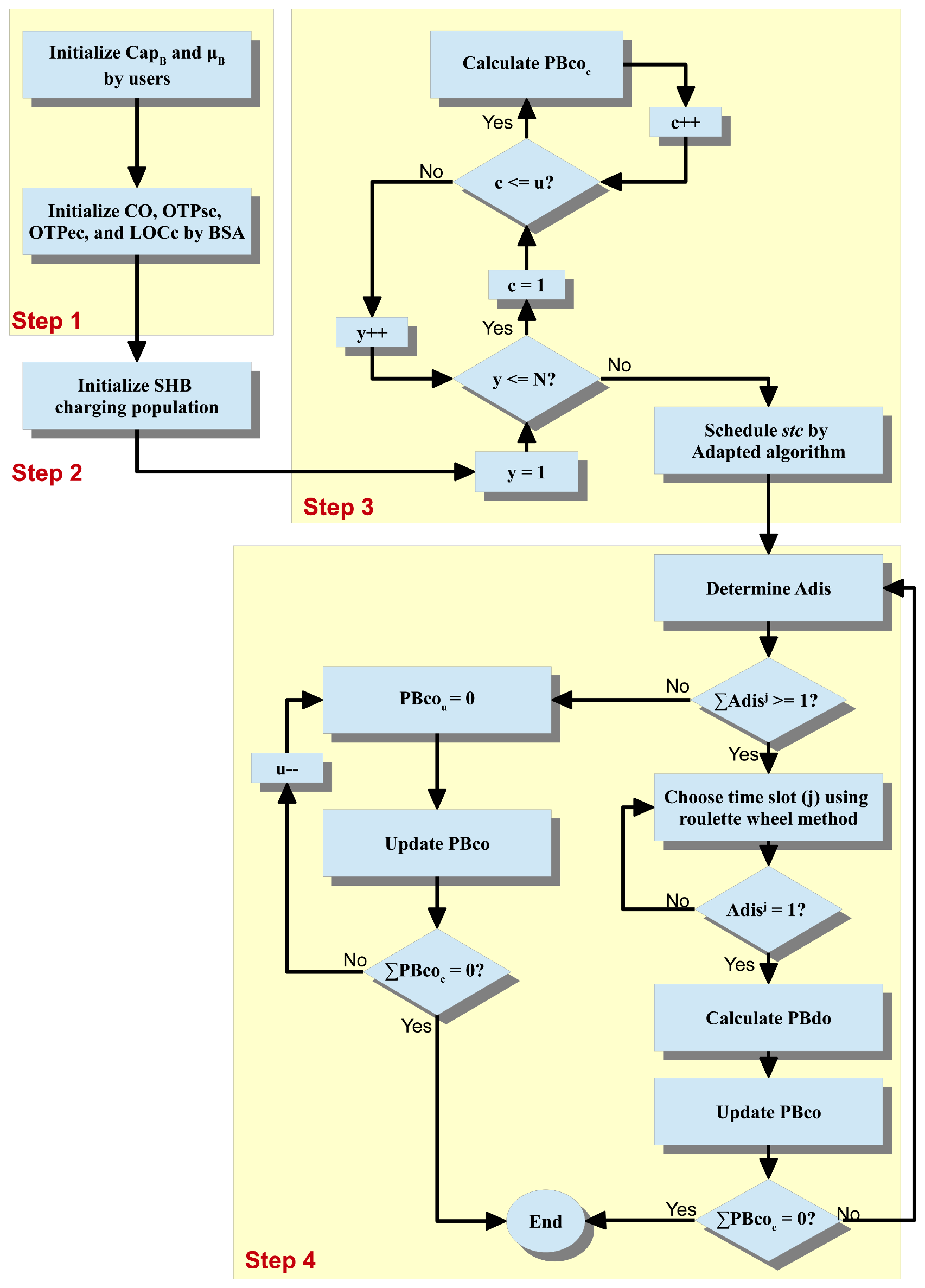
4.2. Smart Home Battery for MO-PSPSH (BMO-PSPSH)

In this section, SHB is modeled to be charged, discharged, and free during the time horizon T. The proposed model of the SHB considers the charging mode as an SA that can be scheduled using the adapted algorithm, while the discharging mode is considered as an additional power source. In the free mode, the SHB is off. The SHB can be scheduled to charge at any time slot considering the available amount of power that can be discharged (i.e., the amount of power charged should not exceed the available amount of power that can be discharged). Besides, the SHB can be discharged at any time slot considering the charging mode and the amount of power charged (i.e., the SHB cannot be discharged at any charged time slot, and the discharged power must not exceed the power charged in SHB). The SHB is modeled to be fully discharged at the end of the time horizon (i.e., no power will transfer to the next time horizon) to evaluate each scenario separately. The SHB is modeled alongside the MO-PSPSH (BMO-PSPSH) to improve its solution(s) and achieve the objectives optimally. The SHB scheduling algorithm (BSA) is developed in this section to manage the modes of the SHB and control amounts of charging and discharging power. The proposed BSA has four main steps, which will be thoroughly discussed below. The flowchart of BSA is provided in Figure 3.

Step  1:

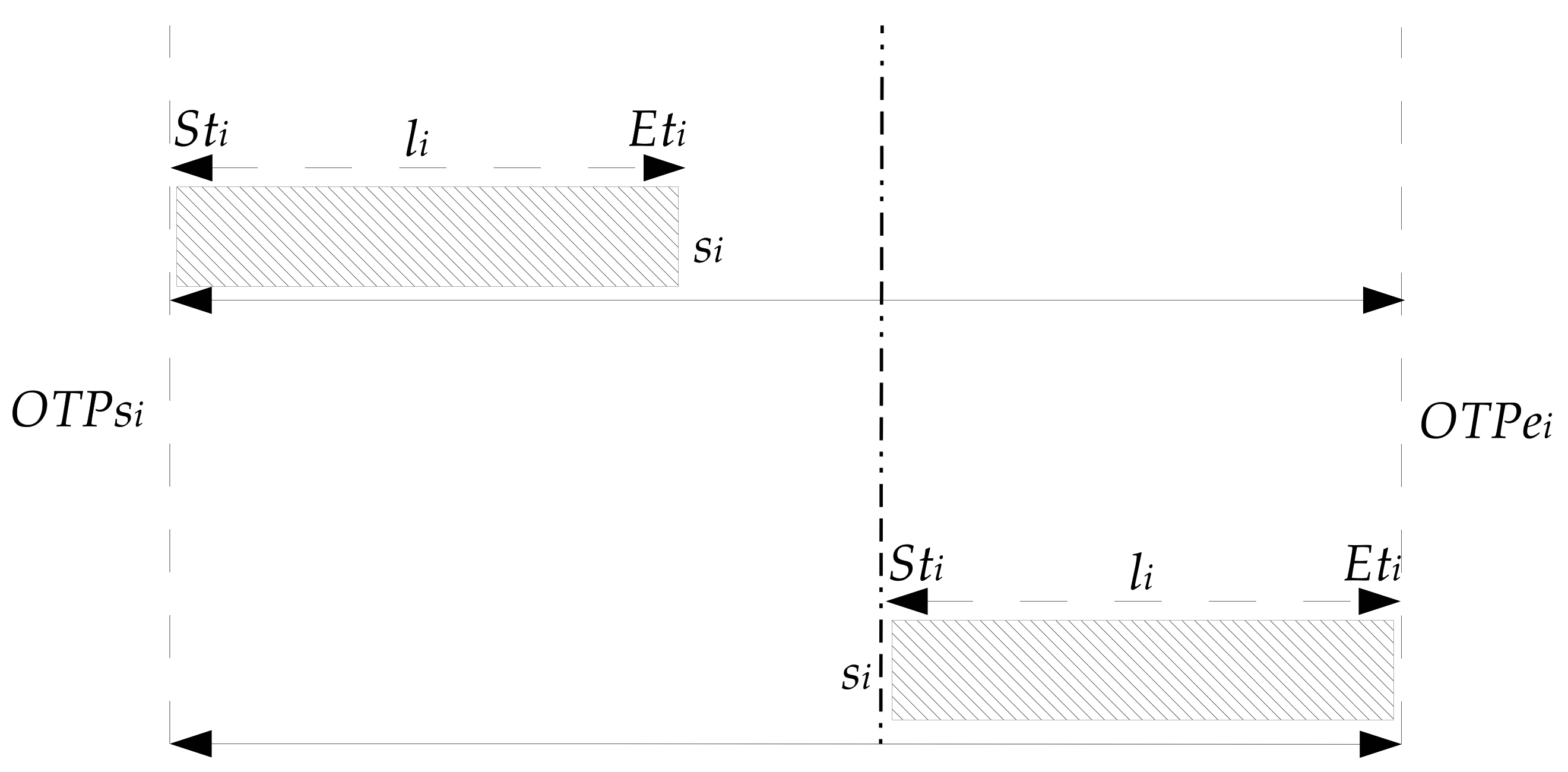
Initialize the SHB parameters

As discussed previously, the charging operations of SHB will be scheduled as SAs in the smart home. Several SHB parameters should be initialized, including the maximum amount of power that can be stored in SHB, known as the capacity of SHB ($Ca{p}_B$), the charging and discharging efficiency, known as the round trip of SHB efficiency (${\mu }_B$), the number of charging operations (CO) represented as $CO=(c{o}_1,c{o}_2,\dots ,c{o}_u)$, the beginning and ending OTP of each charging operation $OTPsc$ and $OTPec$ represented as $OTPsc=(OTPs{c}_1,OTPs{c}_2,\dots ,OTPs{c}_u)$ and $OTPec=(OTPe{c}_1,OTPe{c}_2,\dots ,OTPe{c}_u)$ respectively, and LOC for each charging operation ($LOCc$), such that $LOCc=(l{c}_1,l{c}_2,\dots ,l{c}_u)$. The $Ca{p}_B$ and ${\mu }_B$ are initialized by users, whereas CO, $OTPsc$, $OTPec$, and $LOCc$ are initialized by the proposed BSA.

A constraint of the total number of COs (u) should be considered in this step as follows:

$$Ach=n/2$$

(30)

$$Ach\ge u,$$

(31)

where $Ach$ denotes the number of possible time slots for SHB to be charged. Note that $Ach$ is equal to half of T to keep enough time slots for SHB to be discharged. u is generated randomly in [1, $Ach$].

$OTPsc$ and $OTPec$ for each CO are initialized to be the beginning and ending, respectively, of the available period for SHB to be charged. $OTPsc$ is set to the beginning of T, and $OTPec$ is set to $n-1$ to ensure that SHB not charging at the last time slot. For $LOCc$, each $lc$ is set to be one-time slot (the smallest period to be scheduled).

Algorithm 1 shows the pseudocode for initializing the SHB parameters.

Algorithm 1 Pseudocode of SHB parameters initialization

Parameters initialized by users ($Ca{p}_B,{\mu }_B$) Parameters initialized by BSA ($CO,OTPsc,OTPec,LOCc$) with respecting the $Ach$ Return SHB parameters;

Step  2:

Initialize the SHB charging population

Each solution of charging operations is represented as a vector containing the starting time for each charging operation ($stc$). The population of charging operations contains an N number of solutions initialized randomly, as shown in Equation (32).

$$\begin{array}{cc}\hfill \mathit{SHB}\mathit{charging}\mathit{population}=& \left[\begin{array}{cccc}st{c}_1^1& st{c}_2^1& \cdots & st{c}_u^1\\ st{c}_1^2& st{c}_2^2& \cdots & st{c}_u^2\\ ⋮& ⋮& \cdots & ⋮\\ st{c}_1^N& st{c}_2^N& \cdots & st{c}_u^N\end{array}\right],\end{array}$$

(32)

Algorithm 2 shows the pseudocode for generating the SHB charging population.

Algorithm 2 Pseudocode for generating the SHB charging population

Create a charging operations population matrix of size ($u\times N$) for each solution (y) do for each charging operation (c) do Initialize the values ($stc$) randomly with respecting $OTPsc$, $OTPec$, and $LOCc$ of c end for end for Return SHB charging population;

Step  3:

Calculate the power consumed by the SHB charging operations

In this step, the power charged in SHB by charging operation c at time slot j ($PBc{o}_c^j$) is calculated. $PBco$ can be calculated as follows:

$$PBc{o}_c^j={\mu }_{ch}\times Pc{h}_c^j,$$

(33)

where $Pc{h}_c^j$ is the power consumed by charging operation c at time slot j, which is generated randomly in [0, $C-P{S}_{avg}$] to ensure that it will be within the C or exceed it in the low margin, and ${\mu }_{ch}$ is the SHB charging efficiency. $Pc{h}_c^j$ should not exceed the maximum allowable charge $C{H}^j$ at time slot j, as presented in Equation (34).

$$0\le Pc{h}_c^j\le C{H}^j,$$

(34)

where

$$C{H}^j=CH\times h,$$

where $CH$ is the maximum allowable charge and h is the length of a time slot in hours. In addition, to ensure that the stored power in SHB will not exceed the capacity of SHB, a constraint is formulated as follows:

$$\sum _{c=1}^{u}PBc{o}_c\le Ca{p}_B,$$

(35)

u and $Pch$ are generated randomly by the BSA to increase their flexibility and allow the adapted algorithm to deal with the four objectives of PSPSH. After the PBco for all COs are calculated, the BSA will send COs to the adapted algorithm to be scheduled.

Algorithm 3 shows the pseudocode for calculating the power consumed by the SHB charging operation.

Algorithm 3 Pseudocode for calculating power consumed by the charging operation

for each solution (y) do for each charging operation (c) do Calculate the power consumed based on Equations (33)–(35) end for end for Return charged SHB Return $PBco$ for all $COs$ Send $COs$ to the adapted algorithm to be scheduled

Step  4:

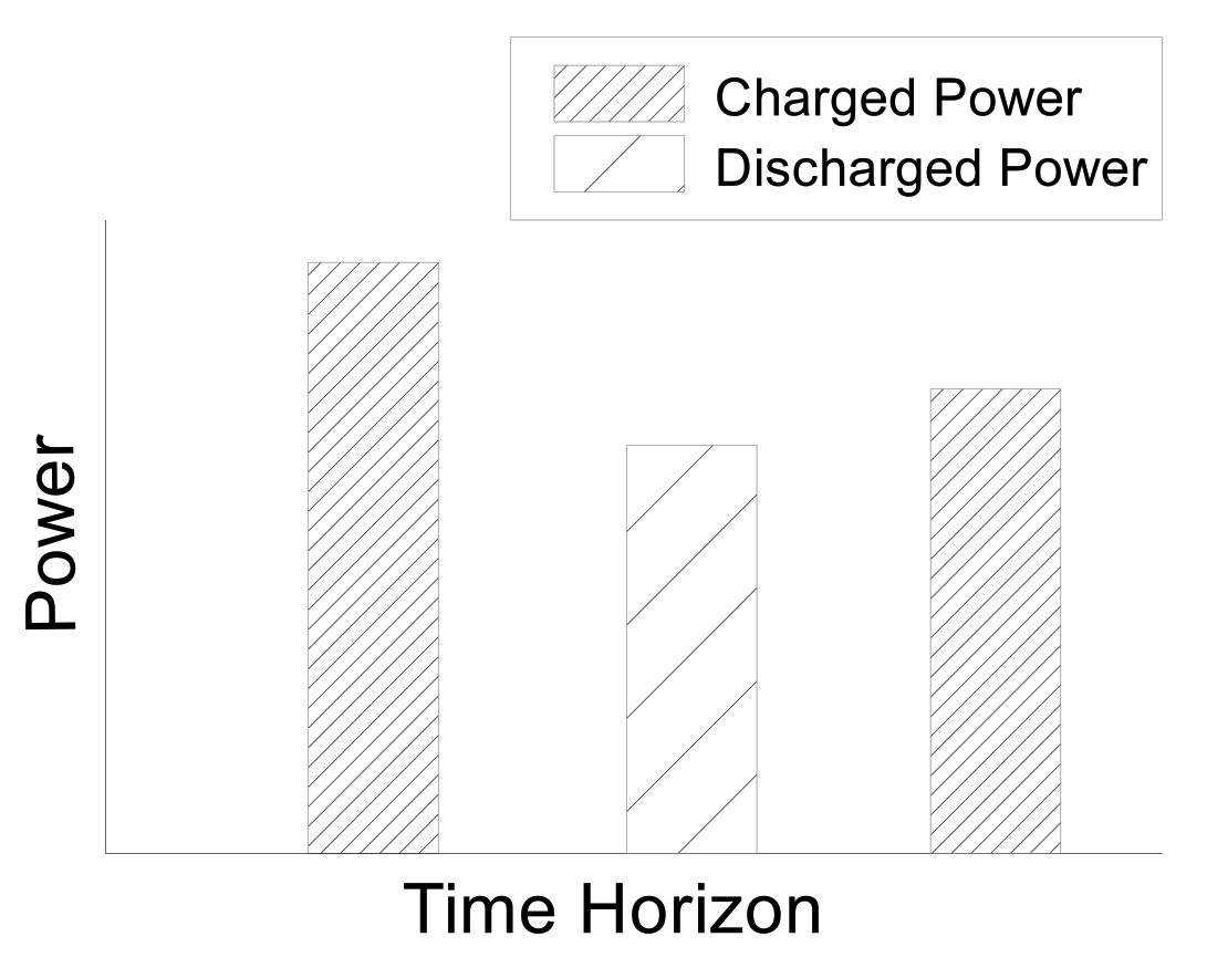
Discharge the SHB

As mentioned previously, the discharging mode of SHB is considered as an additional source. In other words, discharging operations will not be scheduled by the adapted algorithm. However, the discharging mode is managed by the BSA to discharge power using the roulette wheel method, where the charged power will be discharged on the basis of the sizes of the parts on the wheel assigned for each time slot with considering the amount of power consumed at that time slots. In the roulette wheel method, big parts are assigned to high-pricing time slots and small parts to low-pricing time slots. The reason for assigning the part sizes this way in the distribution is to reduce the amount of power consumed at high-pricing time slots due to its effect on the stability of the power system and EBs. The roulette wheel method is used in this study due to its popularity and its performance in distributing individuals on the basis of their importance. Therefore, it gives a high chance for BSA to reduce the amount of power consumed at high-pricing time slots.

The possible time slots for SHB to be discharged is calculated using Equation (36).

$$Adi{s}^j=\left\{\begin{array}{c}1\mathrm{if}P{S}^j>0\mathrm{and}PBc{o}^j=0\mathrm{and}\sum _{b=1}^{j}PBc{o}^b>0\hfill \\ 0\mathrm{Otherwise}\hfill \end{array}\right.,$$

(36)

where $Adis$ denotes the available time slots for SHB to be discharged, $Adi{s}^j$ is equal to 1 if SHB is able to discharge at time slot j and is 0 otherwise, $PBc{o}^j$ can be 0 if SHB is not in the charging mode at time slot j, and ${\sum }_{b=1}^{j}PBc{o}^b>0$ to ensure that SHB is not empty at time slot j.

After choosing a time slot to discharge SHB using the roulette wheel method, BSA will define the amount of power to discharge $PBdo$ on the basis of the power consumed at that time slot as follows:

$$PBd{o}^j={\mu }_{dis}\times Pdi{s}^j,$$

(37)

where $Pdi{s}^j$ is the amount of power that will be discharged from SHB at time slot j, which is generated randomly in [0, $P{S}^j$], and ${\mu }_{dis}$ is the SHB discharging efficiency.

$Pdi{s}^j$ will be released from SHB on the basis of Equation (38). BSA will keep choosing the discharging time slots and update the value of $Adis$ until all of the power stored in SHB is discharged.

$$\sum _{c=1}^u\sum _{b=1}^{j}PBc{o}_c^b=\sum _{c=1}^u\sum _{b=1}^{j-1}PBc{o}_c^b-Pdi{s}^j,$$

(38)

subject to:

$$\sum _{c=1}^u\sum _{b=1}^{j-1}PBc{o}_c^b\ge Pdi{s}^j,$$

However, if the value of ${\sum }_{j=1}^{n}Adi{s}^j$ is equal to 0 and some power is still considered as stored in SHB, then BSA will update the power of the last CO (i.e., $PBc{o}_u$) to be equal to 0 and release it from SHB. The BSA will repeat this process until all of the remaining power in SHB is released

$Pdi{s}^j$ should not exceed the maximum allowable discharge $DI{S}^j$ at time slot j as follows:

$$0\le PBd{o}^j\le DI{S}^j,$$

(39)

where

$$DI{S}^j=DIS\times h,$$

DIS is the maximum allowable discharge. Note that the capacity of any SHB is defined according to the amount of power that can be discharged and not the amount that can be stored. For instance, the capacity of an SHB is 5 kWh, but the usable power is 4.5 kWh. Therefore, ${\mu }_{ch}$ of the proposed SHB is set equal to ${\mu }_B$, while the ${\mu }_{dis}$ is set equal to 1 [74].

Algorithm 4 shows the pseudocode of the discharging power.

Algorithm 4 Pseudocode of discharge the SHB

while$PBco>0$do Determine $Adis$ if${\sum }_{j=1}^{n}Adi{s}^j\ge 1$then Choose the discharging time slot j using roulette wheel method Discharge SHB based on the Equations (37)–(39) else Release $PBc{o}_u$ from $PBco$ end if end while Return SHB discharged;

Algorithm 5 shows the pseudocode of the four steps of the proposed BSA.

Algorithm 5 Pseudocode of the four steps of the proposed BSA

Step  1: Initialize the SHB parameters Parameters initialized by users ($Ca{p}_B,{\mu }_B$) Parameters initialized by BSA ($CO,OTPsc,OTPec,LOCc$) with respecting the $Ach$ Step  2: Initialize the SHB charging population Create a charging operations population matrix of size ($u\times N$) for each solution (y) do for each charging operation (c) do Initialize the values ($stc$) randomly with respecting $OTPsc$, $OTPec$, and $LOCc$ of c end for end for Step  3: Calculate the power consumed by charging operations for each solution (y) do for each charging operation (c) do for each time slot (j) do Calculate the power consumed based on Equations (33)–(35) end for end for end for Send $COs$ to the adapted algorithm to be scheduled Step  4: Discharge the SHB while$PBco>0$do Determine $Adis$ if${\sum }_{j=1}^{n}Adi{s}^j\ge 1$then Choose the discharging time slot j using roulette wheel method Discharge the SHB based on the Equations (37)–(39) else Release $PBc{o}_u$ from $PBco$ end if end while Return empty SHB;

5. Grey Wolf Optimizer for PSPSH

In this section, a swarm-based meta-heuristic optimization algorithm known as the grey wolf optimizer (GWO) algorithm is illustrated and adapted for MO-PSPSH and BMO-PSPSH. The GWO is adapted due to its powerful operations managed by its dynamic parameters to maintain the exploration and exploitation and avoid stagnation in local optima. Furthermore, GWO has a high ability to explore search spaces on the basis of the behavior of its solutions that allow it to search more deeply to find a better solution [12].

5.1. Grey Wolf Optimizer (GWO)

The GWO behavior is inspired mainly by the grey wolves hunting mechanism, and it was mathematically formulated in 2014 by Mirjalili [53].

• Social Hierarchy
  • The pack of grey wolves has an austere social hierarchy, which is classified into alpha ($\alpha$), beta ($\beta$), delta ($\delta$), and omega ($\omega$). Wolves belong to the class alpha are considered as the leader of the grey wolves’ hierarchy due to their domination and power to manage the pack. The beta wolves are playing the primary role in support the alpha in leading the pack. Delta wolves are in the third level of the hierarchy, and they in charge of leading the lowest level in the hierarchy. Omega wolves are considered as the lowest level in the hierarchy.
    In GWO, the solutions are represented as grey wolves in the social hierarchy, where the best solution is represented as $\alpha$ wolf, $\beta$ and $\delta$ wolves are the second and third best solutions, respectively, and $\omega$ wolves are considered as the rest of the solutions.
• Encircling Prey
  • In addition to this deep social hierarchy, the intelligent behavior of group hunting is also procedurally modeled. This behavior involves three main phases: chasing, encircling, and attacking.
    The grey wolves can change/update their locations closer to the prey by encircling the prey mechanism. The encircling behavior of grey wolves is formulated as follows:

    $$\overrightarrow{D}=|\overrightarrow{C}\times {\overrightarrow{X}}_p\left(itr\right)-\overrightarrow{X}\left(itr\right)|,$$

    (40)

    $$\overrightarrow{X}(itr+1)={\overrightarrow{X}}_p\left(itr\right)-\overrightarrow{A}\times \overrightarrow{D},$$

    (41)

    where $\overrightarrow{C}$ and $\overrightarrow{A}$ denote coefficient vectors, $\overrightarrow{X}$ is the grey wolf position vector, ${\overrightarrow{X}}_p$ is the prey position vector, and $itr$ is the current iteration.
    The coefficient vectors $\overrightarrow{C}$ and $\overrightarrow{A}$ are calculated as

    $$\overrightarrow{A}=2\times \overrightarrow{a}\times {\overrightarrow{r}}_1-\overrightarrow{a},$$

    (42)

    $$\overrightarrow{C}=2\times {\overrightarrow{r}}_2,$$

    (43)

    where $\overrightarrow{a}$ is linearly decreased from 2 to 0 throughout iterations and ${\overrightarrow{r}}_1$, ${\overrightarrow{r}}_2$ are random vectors in range of 0 and 1. Based on the values of $\overrightarrow{a}$, the value range of $\overrightarrow{A}$ is between $-2a$ and $2a$.
• Search for Prey (Exploration)
  • The grey wolves searching mechanism for prey can be done on the basis of the wolves’ positions, where the wolves diverge and converge to find the best position to attack prey. The coefficient vectors $\overrightarrow{A}$ and $\overrightarrow{C}$ manage the divergence (exploration) and convergence (exploitation) of the wolves in GWO. GWO exploit a search space if $|\overrightarrow{A}|<1$ and explore a search space if $|\overrightarrow{A}|>1$.
    The changing values in $\overrightarrow{C}$ is not similar to $\overrightarrow{A}$, where $\overrightarrow{C}$ is changing randomly to emphasize exploration/exploitation and local optima stagnation avoidance throughout iterations.
• Hunting
  • As mentioned previously, in GWO, the best three solutions are $\alpha$, $\beta$, and $\delta$ wolves, respectively, and $\omega$ wolves are the rest of the solutions.
    Owing to the domination and leadership of $\alpha$ wolf on the pack, $\alpha$ usually guides the hunting. $\beta$ and $\delta$ wolves occasionally can engage in hunting to help $\alpha$ wolf. $\omega$ wolves are usually changing their location according to the three best solutions ($\alpha ,\beta$, and $\delta$).
    The hunting mechanism on the basis of these wolves (solutions) is formulated as follows:

    $${\overrightarrow{D}}_{\alpha }=|{\overrightarrow{C}}_1\times {\overrightarrow{X}}_{\alpha }-\overrightarrow{X}|,$$

    (44)

    $${\overrightarrow{D}}_{\beta }=|{\overrightarrow{C}}_2\times {\overrightarrow{X}}_{\beta }-\overrightarrow{X}|,$$

    (45)

    $${\overrightarrow{D}}_{\delta }=|{\overrightarrow{C}}_3\times {\overrightarrow{X}}_{\delta }-\overrightarrow{X}|,$$

    (46)

    $${\overrightarrow{X}}_1={\overrightarrow{X}}_{\alpha }-{\overrightarrow{A}}_1\times {\overrightarrow{D}}_{\alpha },$$

    (47)

    $${\overrightarrow{X}}_2={\overrightarrow{X}}_{\beta }-{\overrightarrow{A}}_2\times {\overrightarrow{D}}_{\beta },$$

    (48)

    $${\overrightarrow{X}}_3={\overrightarrow{X}}_{\delta }-{\overrightarrow{A}}_3\times {\overrightarrow{D}}_{\delta },$$

    (49)

    $$\overrightarrow{X}(itr+1)=\frac{{\overrightarrow{X}}_1+{\overrightarrow{X}}_2+{\overrightarrow{X}}_3}{3},$$

    (50)
    To change the location of the $\omega$ wolves for hunting in accordance with the $\alpha ,\beta$ and $\delta$ wolves, the location of the prey should be estimated by these three wolves.

Grey Wolf Optimizer for PSPSH

GWO is a swarm-based optimization algorithm that emphasizes exploration and exploitation using the two parameters (A, C). Besides, GWO can optimally explore the search space using the best three solutions ($\alpha$, $\beta$, $\delta$). Accordingly, GWO is adapted for MO-PSPSH (MO-PSPSH-GWO) and BMO-PSPSH (BMO-PSPSH-GWO) to find the optimal schedule and achieve all PSPSH objectives optimally with and without using SHB. Each solution is evaluated on the basis of the objective function formulated in Equation (29). The GWO adaptation for the two approaches is illustrated in the sections below.

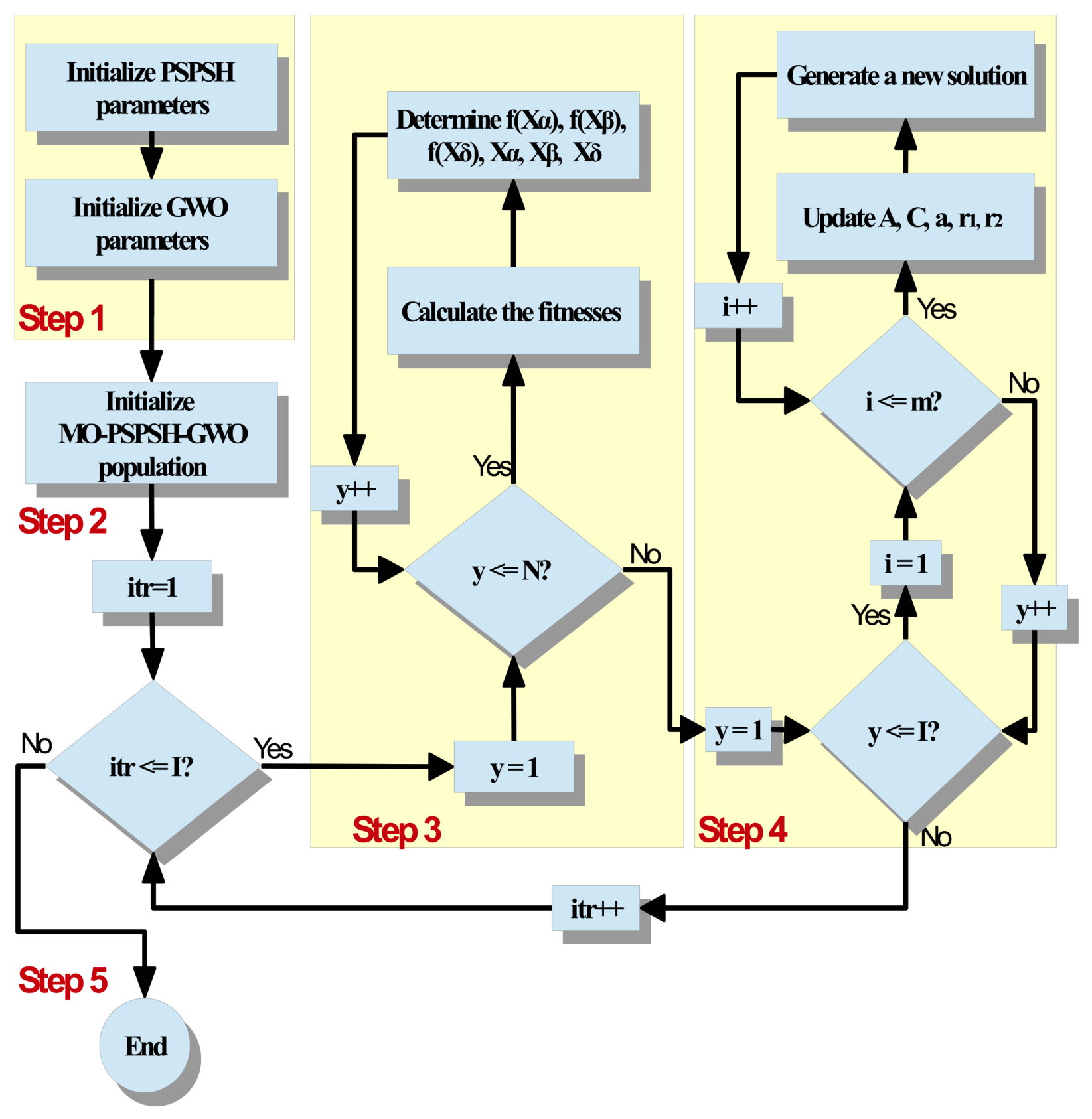
• GWO adaptation for MO-PSPSH (MO-PSPSH-GWO)
  The adaptation of the GWO for MO-PSPSH is discussed in this section. This adaptation contains five main steps, which are illustrated below.
  The flowchart of the proposed MO-PSPSH-GWO is provided in Figure 4.

  Step  1:

  Initialize MO-PSPSH-GWO parameters

  The adaptation the MO-PSPSH-GWO is started by initializing the parameters of PSPSH and GWO. The PSPSH parameters are $\mathbf{S}$, $\mathbf{NS}$, $\mathbf{T}$, $\mathbf{PS}$, $\mathbf{PNS}$, $\mathbf{LOC}$, $\mathbf{OTPs}$, $\mathbf{OTPe}$, and $\mathbf{pc}$. The GWO parameters are $\overrightarrow{A}$, $\overrightarrow{C}$, $\overrightarrow{a}$, $\overrightarrow{r_1}$, $\overrightarrow{r_2}$, the minimum ($lb$) and maximum ($ub$) ranges for the search agent, the maximum number of iterations ($\mathbf{I}$), and the number of search agents in the pack ($\mathbf{N}$).

  Step  2:

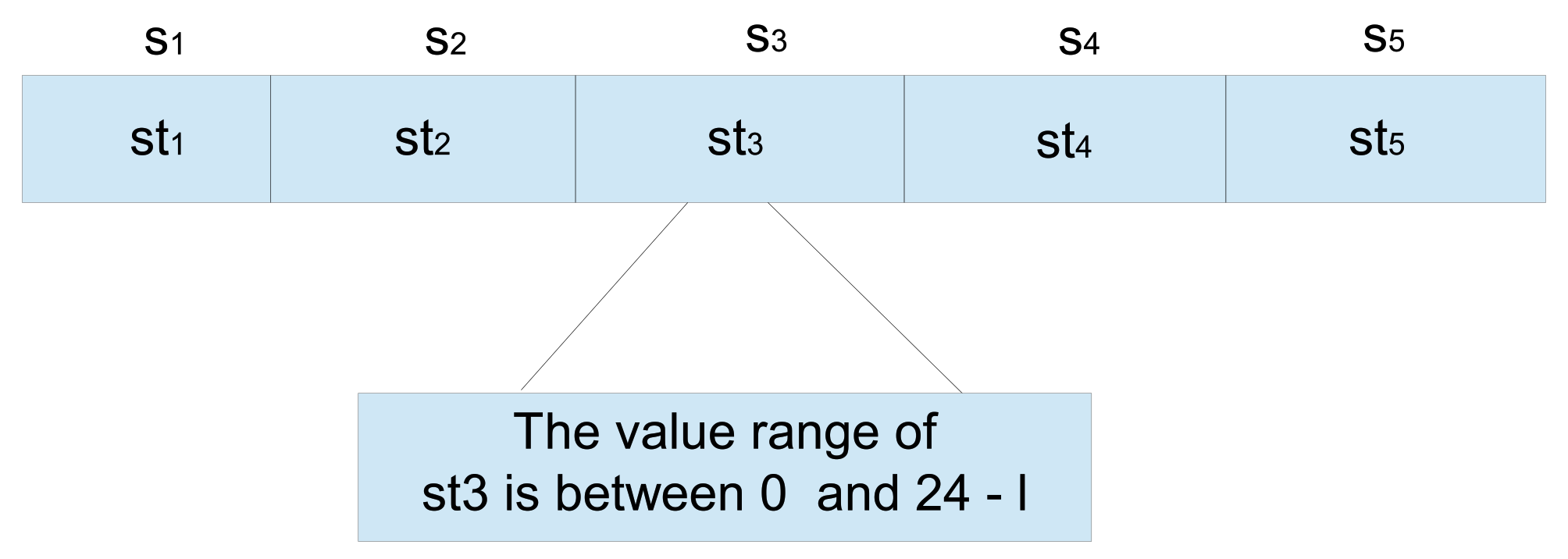
  Initialize MO-PSPSH-GWO population

  Each wolf in the pack is presented as a solution of MO-PSPSH-GWO, and each solution is containing the starting time $st$ for each appliance i, as shown in Figure 5.

  The MO-PSPSH-GWO population is containing of y number of solutions initialized randomly as shown in Equation (51).

  $$\begin{array}{cc}\hfill \mathit{MO}\text{-}\mathit{PSPSH}\text{-}\mathit{GWO}\mathit{population}=& \left[\begin{array}{cccc}s{t}_1^1& s{t}_2^1& \cdots & s{t}_m^1\\ s{t}_1^2& s{t}_2^2& \cdots & s{t}_m^2\\ ⋮& ⋮& \cdots & ⋮\\ s{t}_1^y& s{t}_2^y& \cdots & s{t}_m^y\end{array}\right],\end{array}$$

  (51)

  Step  3:

  Fitness function calculation

  The fitness value of each solution is calculated on the basis of Equation (29). In the MO-PSPSH-GWO method, the best solution and its fitness value are assigned to $X_{\alpha }$ and $f\left(X_{\alpha }\right)$,respectively, and the second and third best solutions and their fitness values are assigned to $X_{\beta }$, $X_{\delta }$, and $f\left(X_{\beta }\right)$, $f\left(X_{\delta }\right)$, respectively.

  Step  4:

  Update the MO-PSPSH-GWO population

  The MO-PSPSH-GWO population is updated in the step, where the Equations (42)–(50) are in charge of this update.

  The updating mechanism of MO-PSPSH-GWO is utilized to estimate the distance between $X_{\omega }$ solutions and the $X_{\alpha }$ solution and then generate a new solution ${\overrightarrow{X}}_1$ Equations (42)–(44) and (47). The same steps for $X_{\alpha }$ are repeated for $X_{\beta }$ and $X_{\delta }$ to generate ${\overrightarrow{X}}_2$ using Equations (42), (43), (45) and (48) and to generate ${\overrightarrow{X}}_3$ using Equations (42), (43), (46) and (49). In Equation (50), a new solution $X^{\prime }(itr+1)$ is generated based on ${\overrightarrow{X}}_1$, ${\overrightarrow{X}}_2$, and ${\overrightarrow{X}}_3$.

  Step  5:

  Check the stop criterion

  Steps 3 and 4 of MO-PSPSH-GWO are repeated until the stop criterion is met.

  Algorithm 6 presents the pseudocode of the five steps of the proposed MO-PSPSH-GWO.

  Algorithm 6 Pseudocode of the five steps of the proposed MO-PSPSH-GWO

  1: Step  1: Initialize MO-PSPSH-GWO parameters;/ 2: Initialize all PSPSH parameters ($S,NS,T,PS,PNS,OT{P}_s,OT{P}_e,LOC,pc$) 3: Initialize all GWO parameters ($a,r_1,r_2\overrightarrow{A},\overrightarrow{C},lb,ub,I,N$) 4: Step  2: Initialize MO-PSPSH-GWO population 5: Initialize MO-PSPSH-GWO population matrix of size ($m\times N$) 6: Step  3: Social Hierarchy 7: while (itr $<=$ I) do 8:  for each solution (y) do 9:   Calculate the fitness of each solution 10:   $f\left(X_{\alpha }\right)$ = the best fitness value 11:   $f\left(X_{\beta }\right)$ = the second fitness value 12:   $f\left(X_{\delta }\right)$ = the third fitness value 13:   $X_{\alpha }$ = the best solution 14:   $X_{\beta }$ = the second best solution 15:   $X_{\delta }$ = the third best solution 16:  end for 17:  Step  4: Update MO-PSPSH-GWO population 18:  for each solution (y) do 19:   for each appliance (i) do 20:    Update $r_1,r_2$ (Random number in [0, 1]) 21:    Update the value of $A_1$ (Equation (42)) 22:    Update the value of $C_1$ (Equation (43)) 23:    Calculate $X_1$ (Equations (44) and (47)) 24:    Update $r_1,r_2$ (Random number in [0, 1]) 25:    Update the value of $A_2$ (Equation (42)) 26:    Update the value of $C_2$ (Equation (43)) 27:    Calculate $X_2$ (Equations (45) and (48)) 28:    Update $r_1,r_2$ (Random number in [0, 1]) 29:    Update the value of $A_3$ (Equation (42)) 30:    Update the value of $C_3$ (Equation (43)) 31:    Calculate $X_3$ (Equations (46) and (49)) 32:    Generate a new solution $X(itr+1)$ (Equation (50)) 33:   end for 34:  end for 35:  Step  5: Check the stop criterion 36:  if The maximum number of the iteration is not reached then 37:   $t=t+1$ 38:  end if 39: end while 40: Return $f\left(X_{\alpha }\right)$ and $X_{\alpha }$

• GWO adaptation for BMO-PSPSH (BMO-PSPSH-GWO)
  BMO-PSPSH-GWO has six main steps, which will be thoroughly discussed below.
  The flowchart of BMO-PSPSH-GWO is provided in Figure 6.

  Step  1:

  Initialize BMO-PSPSH-GWO parameters

  The adaptation of BMO-PSPSH-GWO is started by initializing the parameters of SHB, PSPSH, and GWO. The SHB parameters are $Ca{p}_B,{\mu }_B,CO,OTPsc,OTPec,$ and $LOCc$. The PSPSH and GWO are the same as initialized in the first step of MO-PSPSH-GWO, including $\mathbf{S},\mathbf{NS},\mathbf{T},\mathbf{PS},\mathbf{PNS},\mathbf{LOC},\mathbf{OTPs},\mathbf{OTPe},$ and $\mathbf{pc}$ for PSPSH and $\mathbf{I},\mathbf{N},\overrightarrow{A},\overrightarrow{C},\overrightarrow{a},\overrightarrow{r_1},\overrightarrow{r_2},lb,$ and $ub$ for GWO.

  Step  2:

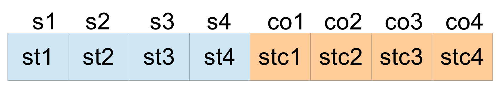
  Initialize BMO-PSPSH-GWO population

  In this step, BMO-PSPSH-GWO solutions are initialized randomly, where each solution is presented as two vectors. The first vector contains the starting time $st$ for SAs and second vector contains the starting time $stc$ for charging operations, as shown in Figure 7

  The BMO-PSPSH-GWO population is presented as a matrix of size $(m+u)\times N$, in which m is the number of SAs, u is the number of charging operations, and N is the number of solutions. Equation (52) shows the presentation of the BMO-PSPSH-GWO population.

  $$\begin{array}{cc}\hfill \mathit{BMO}\text{-}\mathit{PSPSH}\text{-}\mathit{GWO}\mathit{population}=& \left[\begin{array}{cccc}s{t}_1^1& s{t}_2^1& \cdots & s{t}_{m+u}^1\\ s{t}_1^2& s{t}_2^2& \cdots & s{t}_{m+u}^2\\ ⋮& ⋮& \cdots & ⋮\\ s{t}_1^N& s{t}_2^N& \cdots & s{t}_{m+u}^N\end{array}\right]\end{array}$$

  (52)

  Step  3:

  Calculate the power consumed by the charging operations

  In this step, the power charged in SHB by each charging operation will be calculated as discussed in the third step of designing BSA in Section 4.2.

  Step  4:

  Calculate the fitness values

  This step is divided into two parts, namely, discharging the SHB and calculating the fitness values of the solution in the population. As discussed in Section 4.2, the time slots for discharging the SHB are determined using the roulette wheel method and the amount of power chosen randomly on the basis of several equations and constraints. In this step, the processes of discharging the SHB are the same as discussed in Section 4.2. For calculating the fitness values, the three best fitness values and their solutions are assigned as $f\left(X_{\alpha }\right)$, $f\left(X_{\beta }\right)$, and $f\left(X_{\delta }\right)$, and $X_{\alpha }$, $X_{\beta }$, and $X_{\delta }$, respectively.

  Step  5:

  Update BMO-PSPSH-GWO population

  The BMO-PSPSH-GWO population is updated in the step, where the Equations (42)–(50) are in charge of this update.

  The updating mechanism of BMO-PSPSH-GWO is utilized to estimate the distance between $X_{\omega }$ solutions and the $X_{\alpha }$ solution and then generate a new solution ${\overrightarrow{X}}_1$ Equations (42)–(44) and 47. The same steps for $X_{\alpha }$ are repeated for $X_{\beta }$ and $X_{\delta }$ to generate ${\overrightarrow{X}}_2$ using Equations (42), (43), (45) and (48) and to generate ${\overrightarrow{X}}_3$ using Equations (42), (43), (46) and (49). In Equation (50), a new solution $X^{\prime }(itr+1)$ is generated on the basis of ${\overrightarrow{X}}_1$, ${\overrightarrow{X}}_2$, and ${\overrightarrow{X}}_3$.

  Step  6:

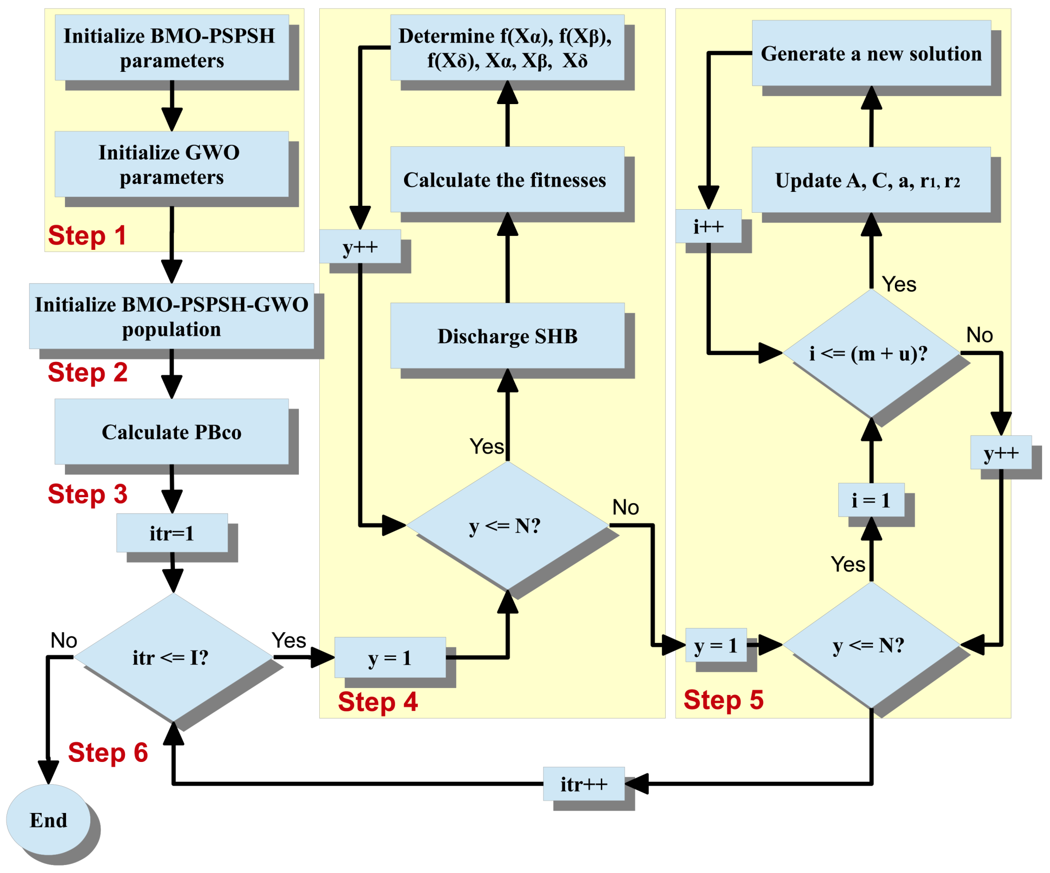
  Check the stop criterion

  Steps 4 and 5 of BMO-PSPSH-GWO are repeated until the stop criterion (maximum number of iterations) is met. The resulting BMO-PSPSH-GWO solution is $X_{\alpha }$.

  Algorithm 7 presents the pseudocode of the six steps of the proposed BMO-PSPSH-GWO.

  Algorithm 7 Pseudocode of the six steps of the proposed BMO-PSPSH-GWO

  1: Step  1: Initialize BMO-PSPSH-GWO parameters 2: Initialize PSPSH parameters($S,NS,T,RS,RNS,OT{P}_s,OT{P}_e,LOC,pc$) 3: Initialized SHB parameters ($Ca{p}_B,{\mu }_B,CO,OTPsc,OTPec,LOCc$) 4: Initialize GWO parameters($a,r_1,r_2\overrightarrow{A},\overrightarrow{C},lb,ub,I,N$) 5: Step  2: Initialize BMO-PSPSH-GWO population 6: Initialize a BMO-PSPSH-GWO population matrix of size ($(m+u)\times N$) 7: Step  3:Calculate the power consumed by charging operations 8: for each solution (y) do 9:  for each charging operation (c) do 10:   Calculate the power consumed based on Equations (33)–(35) 11:  end for 12: end for 13: Step  4: Calculate the fitness values 14: while (itr $<=$ I) do 15:  for each solution (y) do 16:   Discharge the SHB of the solution 17:   Calculate the fitness of the solution 18:   $f\left(X_{\alpha }\right)$ = the best fitness value 19:   $f\left(X_{\beta }\right)$ = the second best fitness value 20:   $f\left(X_{\delta }\right)$ = the third best fitness value 21:   $X_{\alpha }$ = the best solution 22:   $X_{\beta }$ = the second best solution 23:   $X_{\delta }$ = the third best solution 24:  end for 25:  Step  5: Update BMO-PSPSH-GWO population 26:  for each solution (y) do 27:   for each appliance (i) do 28:    Update $r_1,r_2$ (random number in [0, 1]) 29:    Update the value of $A_1$ (Equation (42)) 30:    Update the value of $C_1$ (Equation (43)) 31:    Calculate $X_1$ (Equation (44) and (47)) 32:    Update $r_1,r_2$ (random number in [0, 1]) 33:    Update the value of $A_2$ (Equation (42)) 34:    Update the value of $C_2$ (Equation (43)) 35:    Calculate $X_2$ (Equations (45) and (48)) 36:    Update $r_1,r_2$ (random number in [0, 1]) 37:    Update the value of $A_3$ (Equation (42)) 38:    Update the value of $C_3$ (Equation (43)) 39:    Calculate $X_3$ (Equations (46) and (49)) 40:    Generate a new solution $X(itr+1)$ (Equation (50)) 41:   end for 42:  end for 43:  Step  6: Check the stop criterion 44:  if The maximum number of the iteration is not reached then 45:   $itr=itr+1$ 46:  end if 47: end while 48: Return $f\left(X_{\alpha }\right)$ and $X_{\alpha }$

6. Experiments and Results

The experiments are designed in this section to evaluate the proposed MO-PSPSH and BMO-PSPSH methods using the GWO. MO-PSPSH-GWO and BMO-PSPSH-GWO are evaluated to show their effect in achieving PSPSH objectives. These approaches are compared to show whether BMO-PSPSH-GWO can obtain a better schedule than MO-PSPSH-GWO. For comparison study, the proposed approaches are compared with 17 state-of-the-arts methods using their recommended datasets. Furthermore, the GWO performance is compared with that of GA and PSO to show its performance in achieving the PSPSH objectives.

The proposed methods are implemented and executed using MATLAB on a PC with Intel Core2 Quad CPU, 2.66 GHz processor and 8 GB of memory (RAM).

6.1. Dataset Description

In this study, nine types of SAs are considered for up to 36 operations, where some of these SAs can operate more than once.

The smallest LOC of the SAs is set to 1 minute, where each minute is considered as a time slot in T. Accordingly, the T vector in this dataset is presented as $T=(t_1,t_2,t_3,\dots ,t_{1440})$.

Table 1. Characteristics of the smart home appliances.

NO.	Appliance	l	OTPs–OTPe	Power (kW)	NO.	Appliance	l	OTPs–OTPe	Power (kW)
1	Dishwasher	105	540–780	0.6	19	Dehumidifier	30	1–120	0.05
2	Dishwasher	105	840–1080	0.6	20	Dehumidifier	30	120–240	0.05
3	Dishwasher	105	1200–1440	0.6	21	Dehumidifier	30	240–360	0.05
4	Air Conditioner	30	1–120	1	22	Dehumidifier	30	360–480	0.05
5	Air Conditioner	30	120–240	1	23	Dehumidifier	30	480–600	0.05
6	Air Conditioner	30	240–360	1	24	Dehumidifier	30	600–720	0.05
7	Air Conditioner	30	360–480	1	25	Dehumidifier	30	720–840	0.05
8	Air Conditioner	30	480–600	1	26	Dehumidifier	30	840–960	0.05
9	Air Conditioner	30	600–720	1	27	Dehumidifier	30	960–1080	0.05
10	Air Conditioner	30	720–840	1	28	Dehumidifier	30	1080–1200	0.05
11	Air Conditioner	30	840–960	1	29	Dehumidifier	30	1200–1320	0.05
12	Air Conditioner	30	960–1080	1	30	Dehumidifier	30	1320–1440	0.05
13	Air Conditioner	30	1080–1200	1	31	Electric Water Heater	35	300–420	1.5
14	Air Conditioner	30	1200–1320	1	32	Electric Water Heater	35	1100–1440	1.5
15	Air Conditioner	30	1320–1440	1	33	Coffee Maker	10	300–450	0.8
16	Washing Machine	55	60–300	0.38	34	Coffee Maker	10	1020–1140	0.8
17	Clothes Dryer	60	300–480	0.8	35	Robotic Pool Filter	180	1–540	0.54
18	Refrigerator	1440	1–1440	0.5	36	Robotic Pool Filter	180	900–1440	0.54

shows the main characteristics of the SAs, including the $LOC$ and $OTP$ of each SA.

As mentioned previously, the RTP scheme is used and combined with the IBR scheme due to the IBR performance in dispersing the power consumption throughout the time horizon. RTP is adopted from the Commonwealth Edison Company between the 1st of June, 2016, and the 7th of June, 2016, for a duration of one week (seven days ⇔ seven scenarios) [12,75].

The main features of the seven scenarios are shown in

Table 2. Main characteristics of the seven scenarios.

Scenarios	Appliances
1	1, 3, 4, 5, 6, 7, 15, 18, 19, 20, 21, 22, 23, 24, 25, 26, 27, 28, 29, 30, 31, 33, 35
2	1, 2, 4, 5, 6, 7, 10, 11, 12, 18, 25, 26, 27, 28, 29, 31, 32, 33, 34, 36
3	3, 4, 5, 6, 7, 8, 9, 10, 11, 12, 13, 14, 15, 18, 23, 24, 25, 26, 27, 28, 31, 32, 33, 34, 35
4	1, 2, 3, 4, 5, 6, 7, 8, 9, 10, 11, 12, 13, 14, 15, 16, 17, 18, 19, 20, 21, 22, 23, 24, 25, 26, 27, 28, 29, 30, 31, 32, 33, 34, 35, 36
5	3, 4, 5, 6, 7, 8, 9, 10, 11, 12, 13, 14, 15, 18, 23, 24, 25, 26, 27, 28, 31, 32, 33, 34, 35
6	1, 2, 3, 8, 9, 10, 11, 12, 18, 19, 20, 21, 22, 23, 24, 25, 26, 27, 28, 29, 30, 31, 33, 34, 35
7	1, 3, 4, 5, 6, 7, 8, 9, 10, 11, 12, 13, 14, 15, 16, 17, 18, 19, 20, 21, 22, 23, 24, 25, 26, 27, 28, 29, 30, 31, 33, 34, 35, 36

. In this table, the columns “Scenarios” and “Appliances” are referring to the scenario number and the appliances’ number in Table 1. For example, number 1 and 36 in the appliances’ column in Table 2 refers to the first (Dishwasher) and last (Robotic Pool Filter) appliances in Table 1. Appliances used in scenario #1 are 1, 3, 4, 5, 6, 7, 15, 18, 19, 20, 21, 22, 23, 24, 25, 26, 27, 28, 29, 30, 31, 33, 35.

Table 3. Non-shiftable appliances (NSAs) used in the simulation.

No.	Appliances	Power (kW)
1	Light [16]	0.6
2	Attic Fan [76]	0.3
3	Table Fan [76]	0.8
4	Iron [16]	1.5
5	Toaster [76]	1
6	Computer Charger [76]	1.5
7	Cleaner [15]	1.5
8	TV [76]	0.3
9	Hair Dryer [76]	1.2
10	Hand Drill [76]	0.6
11	Water Pump [76]	2.5
12	Blender [76]	0.3
13	Microwave [16]	1.18
14	Electric Vehicle [77]	1

shows the NSAs used in this study and their power. Given that all NSAs are operated manually by users, nobody can predefine their time parameters, including $OT{P}_s$, $OT{P}_e$, and LOC.

For the GWO parameters, the algorithm run 1000 iterations in each run since the 1000 generations are enough for convergence of algorithms [78].

Table 4. Parameters used in GWO algorithm.

Parameter	Value
N	40
I	1000
lb	$OT{P}_s$
ub	$OT{P}_e-LOC$

presents the parameter setting for the GWO.

The same features of Tesla Powerwall 2 are used for the SHB in this study [79].

Table 5. SHB parameters.

Parameter	Value
$Ca{p}_B$	13.5 kWh
$C{H}_{max}$	5 kW
$DI{S}_{max}$	5kW
${\mu }_B$	90%

shows the proposed SHB parameters.

6.2. Experimental Evaluation

In this section, the simulation results are presented to show whether the BMO-PSPSH-GWO method can obtain a better schedule than considering the MO-PSPSH-GWO method. The performance of BMO-PSPSH-GWO and MO-PSPSH-GWO on EB, PAR, WTR, and CPR reduction is evaluated and analyzed.

As discussed in Section 3, using the MO-PSPSH each objective assigned with a weight that denoting its importance. Therefore, the weight ($w_1$) assigned to EB is the highest, due to its significance in optimizing PSPSH, where it is the main benefit gaining by users [6]. Accordingly, $w_1$ is assigned by 0.4, and each of $w_2,w_3,$ and $w_4$ assigned by 0.2 (Equation (29)).

6.2.1. Effect of The Proposed Approaches on EB

The effect of BMO-PSPSH-GWO and MO-PSPSH-GWO on EB reduction is presented in this section. The results of BMO-PSPSH-GWO are compared with MO-PSPSH-GWO to investigate whether the proposed SHB can improve the solution in terms of reducing EB. EB obtained by these approaches is compared in

Table 6. Comparison between MO-PSPSH-GWO and BMO-PSPSH-GWO in terms of electricity bill (EB) reduction.

Scenarios	MO-PSPSH-GWO	BMO-PSPSH-GWO
S 1	43.5041	41.9042
S 2	64.5597	59.6252
S 3	66.1138	62.7707
S 4	62.5916	55.9692
S 5	46.2879	43.6999
S 6	52.2998	49.1431
S 7	62.6367	56.4908
Average	56.8562	52.8004
Total	397.993	369.603

Bold values indicate the best values.

. The table shows EB obtained by the two approaches for the seven scenarios, a comparison between the two approaches in terms of average and total EB is shown in the table as well.

BMO-PSPSH-GWO reduces EB better than MO-PSPSH-GWO in all scenarios due to the performance of SHB in reducing EB by scheduling the charging operations of SHB at the best time slots based on Equation (29); i.e., schedule several charging operations at low pricing periods and discharge SHB at high pricing periods.

6.2.2. Effect of The Proposed Approaches on PAR

As shown in the previous section, the proposed BMO-PSPSH-GWO has a high effect in reducing EB because it stores power at low pricing periods and uses the stored power at high pricing periods. In this section, the effect of BMO-PSPSH-GWO on PAR value is presented and compared with PAR value obtained using MO-PSPSH-GWO.

PAR values obtained by the BMO-PSPSH-GWO approach for the seven scenarios are shown in

Table 7. Comparison between MO-PSPSH-GWO, BMO-PSPSH-GWO in terms of peak-to-average ratio (PAR) reduction.

Scenarios	MO-PSPSH-GWO	BMO-PSPSH-GWO
S 1	2.6002	2.9418
S 2	2.4451	2.4796
S 3	2.2267	2.5710
S 4	2.2277	2.3167
S 5	2.2310	2.5207
S 6	2.5233	2.5375
S 7	2.0423	2.4931
Average	2.3280	2.5515

Bold values indicate the best values.

. Besides, the table presents PAR obtained by MO-PSPSH-GWO to show whether MO-PSPSH-GWO or BMO-PSPSH-GWO can reduce PAR values better.

Notably, MO-PSPSH-GWO obtained better PAR values than BMO-PSPSH-GWO in all scenarios due to increasing amount of power consumed by SHB at low pricing period and increase $P{S}_{max}$ value (Equation (14)); therefore, increase PAR values, as shown in Figure 8.

6.2.3. Effect of The Proposed Approaches on UC Level

As discussed previously, the UC level in this study is evaluated on the basis of WTR and CPR. UC level can be improved by reducing the values of the two parameters. The effect of BMO-PSPSH-GWO on UC parameters are presented and compared with MO-PSPSH-GWO in this section.

Table 8. Comparison between MO-PSPSH-GWO and BMO-PSPSH-GWO in terms of waiting time rate (WTR) reduction.

Scenarios	MO-PSPSH-GWO	BMO-PSPSH-GWO
S 1	0.0658	0.0645
S 2	0.1030	0.0534
S 3	0.0889	0.0629
S 4	0.1358	0.0787
S 5	0.0872	0.0695
S 6	0.1004	0.0598
S 7	0.1310	0.0771
Average	0.1017	0.0666

Bold values indicate the best values.

and

Table 9. Comparison between MO-PSPSH-GWO and BMO-PSPSH-GWO in terms of capacity power limit rate (CPR) reduction.

Scenarios	MO-PSPSH-GWO	BMO-PSPSH-GWO
S 1	0.3206	0.3216
S 2	0.3528	0.3529
S 3	0.3913	0.3871
S 4	0.5236	0.5062
S 5	0.3924	0.3880
S 6	0.3647	0.3546
S 7	0.4857	0.4590
Average	0.4044	0.3956

Bold values indicate the best values.

present WTR and CPR values obtained by MO-PSPSH-GWO and BMO-PSPSH-GWO for the seven days, respectively, to show which approach got a better schedule in terms of improving UC level.

Table 8 and Table 9 show the high performance of BMO-PSPSH-GWO in reducing WTR and CPR, where it outperforms MO-PSPSH-GWO in most of the scenarios and their average values. The reduction of WTR is because of BSA’s mechanism that schedules SHB to discharge power at suitable time slots (e.g., time slots at the beginning of OTP) that allow SAs to operate at the beginning of OTP using suitable pricing tariffs. For CPR, its values are reduced because of increasing available power to operate NSAs due to reducing some power exceeds or near the threshold.

The UC level is increased using BMO-PSPSH-GWO by up to 2% compared with MO-PSPSH-GWO, as shown in

Table 10. Comparison between MO-PSPSH-GWO and BMO-PSPSH-GWO in terms of user comfort (UC) percentage (%).

Scenarios	MO-PSPSH-GWO	BMO-PSPSH-GWO
S 1	80.67	80.68
S 2	77.20	79.67
S 3	75.98	77.49
S 4	67.02	70.75
S 5	76.01	77.12
S 6	76.74	79.27
S 7	69.16	73.18
Average	74.68	76.88

Bold values indicate the best value in each scenario.

. In addition, the table shows the UC percentage for the seven scenarios obtained by the two approaches.

6.2.4. Discussion

The performance of BMO-PSPSH-GWO is evaluated against MO-PSPSH-GWO for seven scenarios (1 week). The evaluation is designed to show the proposed approach’s performance in achieving PSPSH objectives. SHB is proposed alongside MO-PSPSH to improve the schedule and mainly enhance the reduction of EB with considering the other objectives reduction. In addition, SHB reduces the amount of power consumed by SAs at unsuitable periods that are conflicting with PSPSH objectives, by storing power at suitable periods and discharge the stored power at the unsuitable periods. The price scheme used in this study is the RTP scheme combined with the IBR scheme. This combination is provided to disperse power consumption throughout the time horizon.

The simulation results show high performance of BMO-PSPSH-GWO, where it outperforms MO-PSPSH-GWO in reducing EB, WTR, and CPR, whereas MO-PSPSH-GWO obtains better result only in reducing the PAR value. However, BMO-PSPSH-GWO does not obtain a better PAR reduction than MO-PSPSH-GWO due to the increasing amount of power consumed at low pricing periods and increase the value $P{S}_{max}$ (Equation (14)).

Note that the cost of the SHB used in this study is not considered due to the four objectives (i.e., EB, PAR, WTR, and CPR) that are affected by the SHB, where it seems hard and impractical to compare its cost with the four objectives values. In addition, the SHB used in this study has an unlimited life cycle; therefore, it can provide benefits for an extensive time.

6.3. Comparative Evaluation

Two types of comparisons are conducted in this study, including comparison with state-of-the-art methods using their datasets, and the most popular metaheuristic optimization algorithms were adapted for PSPSH using the proposed SHB and datasets. The state-of-the-art methods are HSA and BFOA [42], GA, BPSO, and WDO [80], GA and GWO [81], GOA, CSA, ACO, FA, and MFO [82], and GA and DA [83]. The basic metaheuristic optimization algorithms are GA, BFOA, HSA, and PSO [14].

6.3.1. Comparison with State-of-the-Art Methods Using Their Datasets

This section compares the proposed method using SHB with 17 state-of-the-art methods using their recommended datasets. The compared studies used different types of objective functions, including single objective and MO functions. Therefore, the compared studies’ objective functions are considered with the proposed SHB (B-PSPSH-GWO) in this comparison study instead of the BMO-PSPSH approach. The evaluation in this comparison is analyzed on the basis of the values of EB and PAR. UC level is not conducted in this comparison because it was used in the studies based on different criteria.

Table 11. Features of the compared studies. Time-of-use price (TOU)—two seasons.

Study	Method	Appliances	Pricing Scheme	Time Slot
[42]	HSA, BFOA	13	TOU	1 h
[80]	GA, BPSO, WDO	9	RTP	1 h
[81]	GA, GWO	12	RTP, CPP	1 h
[82]	GOA, CSA, ACO, FA, MFO	6	RTP	1 h
[83]	GA, DA	12	RTP	1 h

summarized the features of the compared studies, including the study, method used, number of appliances, pricing scheme used.

Table 12. Comparison between proposed and the comparative methods.

Study	Algorithm	EB	PAR
	HSA	1523.9	2.24
[42]	BFOA	1558.8	2.15
(Summer Scenario)	HBH	1557.2	2.12
	B-PSPSH-GWO	1082.4	2.47
	HSA	1155.8	3.26
[42]	BFOA	1082.9	3.18
(Winter Scenario)	HBH	1143.6	3.5
	B-PSPSH-GWO	954.8	3.7
	GA	64	2.2
	BPSO	42	2
[80]	WDO	41.6	1.9
	GWDO	37	1.7
	B-PSPSH-GWO	30.2	2.28
[81]	GA	462.67	3.639
(RTP Scenario)	GWO	474.06	3.774
	HGWGA	449.35	3.108
	B-PSPSH-GWO	426.18	3.95
	GA	523.96	3.639
[81]	GWO	541.45	3.774
(CPP Scenario)	HGWGA	508.35	3.108
	B-PSPSH-GWO	474.21	3.95
[82]	GOA	1768.27	7.41
	CSA	2147.28	9.47
	ACO	2001.16	4.13
	FA	2104.23	8.02
	MFO	1794.61	8.31
	B-PSPSH-GWO	1673.79	8.50
	GA	1.683	3.56
[83]	DA	1.561	3.76
	B-PSPSH-GWO	1.23	3.94

Bold values indicate the best value in each scenario.

shows the results obtained by the methods in each study and the proposed B-PSPSH-GWO. The results prove the robust performance of the proposed SHB for PSPSH in reducing EB, where the proposed B-PSPSH-GWO shows a significant reduction in EB compared with all other methods. However, as discussed previously, due to the mechanism of the SHB in using power at low peak periods, the power consumed at these periods are higher than the others. Therefore, the PAR value is expected to be increased, which explains the high values of PAR obtained by the proposed B-PSPSH-GWO compared with the other methods.

6.3.2. Comparison with State-of-the-Art Methods Using the Proposed Datasets

This section mainly compares the performance of the GWO with that of GA, PSO, HSA, and BFOA using the proposed SHB for PSPSH. The performance of these algorithms is evaluated on the basis of the PSPSH objectives, including EB, PAR, WTR, and CPR.

The datasets used in this comparison study are presented in Table 1, Table 2 and Table 3.

Table 13. Comparison between the five algorithms in terms of EB reduction.

Scenarios	GWO	GA	PSO	HSA	BFOA
S 1	41.90	44.54	42.05	43.72	42.39
S 2	59.62	62.00	59.76	61.46	60.18
S 3	62.77	65.10	63.01	63.92	63.24
S 4	55.96	56.56	56.14	56.44	56.32
S 5	43.69	47.90	43.77	44.96	43.93
S 6	49.14	52.55	49.21	50.86	49.95
S 7	56.49	59.22	56.60	58.11	57.10
Average	52.80	55.41	52.93	54.21	53.30

Bold values indicate the best value in each scenario.

shows EBs obtained by the GWO, GA, PSO, HSA, and BFOA for seven scenarios. In addition, the average EB obtained by these algorithms are presented.

The GWO proves its high performance in reducing EB, where it achieves the best EB against the other methods.

PAR values obtained by these algorithms are presented in

Table 14. Comparison between the five algorithms in terms of PAR reduction.

Scenarios	GWO	GA	PSO	HSA	BFOA
S 1	2.94	2.96	2.89	2.95	2.94
S 2	2.47	2.57	2.49	2.53	2.50
S 3	2.57	2.92	2.58	2.86	2.61
S 4	2.31	2.33	2.30	2.35	2.33
S 5	2.52	2.73	2.54	2.71	2.59
S 6	2.53	2.70	2.55	2.72	2.65
S 7	2.49	2.65	2.51	2.62	2.54
Average	2.54	2.694	2.55	2.691	2.58

Bold values indicate the best value in each scenario.

. The table shows the robust performance of GWO in dispersing the power consumed through the time horizon, where it achieves the lowest overall PAR compared with the other algorithms.

WTR and CPR values achieved by the five algorithms for the same scenarios are compared in

Table 15. Comparison between the five algorithms in terms of WTR reduction.

Scenarios	GWO	GA	PSO	HSA	BFOA
S 1	0.064	0.102	0.072	0.100	0.084
S 2	0.053	0.135	0.061	0.112	0.076
S 3	0.062	0.100	0.065	0.083	0.069
S 4	0.078	0.142	0.083	0.122	0.089
S 5	0.069	0.098	0.070	0.081	0.080
S 6	0.059	0.088	0.062	0.085	0.077
S 7	0.077	0.110	0.078	0.095	0.091
Average	0.066	0.110	0.070	0.096	0.080

Bold values indicate the best value in each scenario.

and

Table 16. Comparison between the five algorithms in terms of CPR reduction.

Scenarios	GWO	GA	PSO	HSA	BFOA
S 1	0.321	0.340	0.322	0.339	0.328
S 2	0.352	0.361	0.357	0.363	0.357
S 3	0.387	0.401	0.386	0.400	0.390
S 4	0.506	0.519	0.505	0.519	0.510
S 5	0.388	0.411	0.393	0.409	0.399
S 6	0.354	0.370	0.355	0.373	0.361
S 7	0.459	0.469	0.460	0.463	0.463
Average	0.395	0.410	0.396	0.409	0.401

Bold values indicate the best value in each scenario.

. The tables present and prove the robust performance of the GWO in reducing WTR and CPR values, where it obtains the best WTR in all scenarios and the best CPR in five scenarios compared with the other algorithms. In addition, GWO achieves the best overall reduction by obtaining the best average WTR and CPR values. Accordingly, GWO got the highest improvement for UC level, as shown in

Table 17. Comparison between the five algorithms in terms of $U{C}_p$ improvement.

Scenarios	GWO	GA	PSO	HSA	BFOA
S 1	80.68	77.90	80.30	78.05	79.4
S 2	79.67	75.20	79.10	76.25	78.35
S 3	77.49	74.95	77.45	75.85	77.05
S 4	70.75	66.95	70.60	67.95	70.05
S 5	77.12	74.55	76.85	75.50	76.05
S 6	79.27	77.10	79.15	77.10	78.10
S 7	73.18	71.05	73.10	72.10	72.30
Average	76.88	73.95	76.65	74.68	75.90

Bold values indicate the best value in each scenario.

.

This comparison study proves the robust performance of the GWO in addressing PSPSH, where it outperforms all other compared algorithms in achieving PSPSH objectives, including EB, PAR, WTR, and CPR.

7. Conclusions and Future Research

PSPSH refers to a timely schedule of operations of smart home appliances in accordance with a set of restrictions and a dynamic pricing scheme(s). The primary objectives of PSPSH are minimizing EB, PAR, and user discomfort levels. The RTP is combined with the IBR scheme in this study to provide different prices on the basis of time changing and the amount of power consumed. PSPSH is formulated as a MOP (MO-PSPSH) to achieve all objectives simultaneously. SHB can enhance the scheduling of appliances by storing power at unsuitable periods and use the stored power at suitable periods for PSPSH objectives. Therefore, a new formulation for SHB to improve the PSPSH solutions’ quality is provided in this paper.

GWO is adapted to address MO-PSPSH (MO-PSPSH-GWO) and BMO-PSPSH (BMO-PSPSH-GWO) approaches due to its powerful operations managed by its dynamic parameters that maintain exploration and exploitation in search space.

Seven scenarios of power consumption and RTP schemes are considered in the simulation results to evaluate the proposed MO-PSPSH-GWO and BMO-PSPSH-GWO. The results demonstrated the efficiency of BMO-PSPSH-GWO compared with MO-PSPSH-GWO, where it obtains better results in minimizing EB, WTR, and CPR, and improving UC level. However, MO-PSPSH-GWO achieves better PAR values than BMO-PSPSH-GWO. For comparison evaluation, the proposed BMO-PSPSH-GWO compared with 17 state-of-the-art algorithms using their recommended datasets and four algorithms using the proposed datasets. The proposed BMO-PSPSH-GWO exhibits and yields better performance than the other compared algorithms in almost all scenarios.

Possible future directions can use more scenarios and standard datasets to evaluate the proposed approaches robustly. In addition, the GWO can be hybridized with another algorithm to address its defects and exhibits better results for PSPSH.

References

- Fadlullah, Z.M.; Quan, D.M.; Kato, N.; Stojmenovic, I. GTES: An optimized game-theoretic demand-side management scheme for smart grid. IEEE Syst. J. 2014, 8, 588–597. [Google Scholar] [CrossRef]
- Yan, Y.; Qian, Y.; Sharif, H.; Tipper, D. A survey on smart grid communication infrastructures: Motivations, requirements and challenges. IEEE Commun. Surv. Tutor. 2013, 15, 5–20. [Google Scholar] [CrossRef] [Green Version]
- Ayodele, E.; Misra, S.; Damasevicius, R.; Maskeliunas, R. Hybrid microgrid for microfinance institutions in rural areas—A field demonstration in West Africa. Sustain. Energy Technol. Assess. 2019, 35, 89–97. [Google Scholar] [CrossRef]
- Woźniak, M.; Połap, D. Intelligent Home Systems for Ubiquitous User Support by Using Neural Networks and Rule-Based Approach. IEEE Trans. Ind. Inform. 2020, 16, 2651–2658. [Google Scholar] [CrossRef]
- Wozniak, M.; Zielonka, A.; Sikora, A.; Piran, M.J.; Alamri, A. 6G-enabled IoT Home Environment control using Fuzzy Rules. IEEE Internet Things J. 2020. [Google Scholar] [CrossRef]
- Khan, A.R.; Mahmood, A.; Safdar, A.; Khan, Z.A.; Khan, N.A. Load forecasting, dynamic pricing and DSM in smart grid: A review. Renew. Sustain. Energy Rev. 2016, 54, 1311–1322. [Google Scholar] [CrossRef]
- Mostafa, S.A.; Gunasekaran, S.S.; Mustapha, A.; Mohammed, M.A.; Abduallah, W.M. Modelling an adjustable autonomous multi-agent internet of things system for elderly smart home. In Proceedings of the International Conference on Applied Human Factors and Ergonomics; Springer: Berlin/Heidelberg, Germany, 2019; pp. 301–311. [Google Scholar] [CrossRef]
- Venckauskas, A.; Stuikys, V.; Damasevicius, R.; Jusas, N. Modelling of Internet of Things units for estimating security-energy-performance relationships for quality of service and environment awareness. Secur. Commun. Netw. 2016, 9, 3324–3339. [Google Scholar] [CrossRef]
- Makhadmeh, S.N.; Khader, A.T.; Al-Betar, M.A.; Naim, S.; Abasi, A.K.; Alyasseri, Z.A.A. A novel hybrid grey wolf optimizer with min-conflict algorithm for power scheduling problem in a smart home. Swarm Evol. Comput. 2021, 60, 100793. [Google Scholar] [CrossRef]
- Makhadmeh, S.N.; Khader, A.T.; Al-Betar, M.A.; Naim, S.; Alyasseri, Z.A.A.; Abasi, A.K. A min-conflict algorithm for power scheduling problem in a smart home using battery. In Proceedings of the 11th National Technical Seminar on Unmanned System Technology 2019; Springer: Berlin/Heidelberg, Germany, 2020; pp. 489–501. [Google Scholar] [CrossRef]
- Colak, I.; Kabalci, E.; Fulli, G.; Lazarou, S. A survey on the contributions of power electronics to smart grid systems. Renew. Sustain. Energy Rev. 2015, 47, 562–579. [Google Scholar] [CrossRef]
- Makhadmeh, S.N.; Khader, A.T.; Al-Betar, M.A.; Naim, S. Multi-objective power scheduling problem in smart homes using grey wolf optimiser. J. Ambient Intell. Humaniz. Comput. 2019, 10, 3643–3667. [Google Scholar] [CrossRef]
- Ghani, M.K.A.; Mohammed, M.A.; Ibrahim, M.S.; Mostafa, S.A.; Ibrahim, D.A. Implementing an efficient expert system for services center management by fuzzy logic controller. J. Theor. Appl. Inf. Technol. 2017, 95, 13. [Google Scholar]
- Makhadmeh, S.N.; Khader, A.T.; Al-Betar, M.A.; Naim, S.; Abasi, A.K.; Alyasseri, Z.A.A. Optimization methods for power scheduling problems in smart home: Survey. Renew. Sustain. Energy Rev. 2019, 115, 109362. [Google Scholar] [CrossRef]
- Zhao, Z.; Lee, W.C.; Shin, Y.; Song, K.B. An optimal power scheduling method for demand response in home energy management system. IEEE Trans. Smart Grid 2013, 4, 1391–1400. [Google Scholar] [CrossRef]
- Rahim, S.; Javaid, N.; Ahmad, A.; Khan, S.A.; Khan, Z.A.; Alrajeh, N.; Qasim, U. Exploiting heuristic algorithms to efficiently utilize energy management controllers with renewable energy sources. Energy Build. 2016, 129, 452–470. [Google Scholar] [CrossRef]
- Iftikhar, H.; Asif, S.; Maroof, R.; Ambreen, K.; Khan, H.N.; Javaid, N. Biogeography Based Optimization for Home Energy Management in Smart Grid. In Proceedings of the International Conference on Network-Based Information Systems; Springer: Berlin/Heidelberg, Germany, 2017; pp. 177–190. [Google Scholar] [CrossRef]
- Faiz, Z.; Bilal, T.; Awais, M.; Gull, S.; Javaid, N. Demand Side Management Using Chicken Swarm Optimization. In Proceedings of the International Conference on Intelligent Networking and Collaborative Systems; Springer: Berlin/Heidelberg, Germany, 2017; pp. 155–165. [Google Scholar] [CrossRef]
- Asif, S.; Ambreen, K.; Iftikhar, H.; Khan, H.N.; Maroof, R.; Javaid, N. Energy Management in Residential Area using Genetic and Strawberry Algorithm. In Proceedings of the International Conference on Network-Based Information Systems; Springer: Berlin/Heidelberg, Germany, 2017; pp. 165–176. [Google Scholar] [CrossRef]
- Rehman, A.U.; Aslam, S.; Abideen, Z.U.; Zahra, A.; Ali, W.; Junaid, M.; Javaid, N. Efficient Energy Management System Using Firefly and Harmony Search Algorithm. In Proceedings of the International Conference on Broadband and Wireless Computing, Communication and Applications; Springer: Berlin/Heidelberg, Germany, 2017; pp. 37–49. [Google Scholar] [CrossRef]
- Batool, S.; Khalid, A.; Amjad, Z.; Arshad, H.; Aimal, S.; Farooqi, M.; Javaid, N. Pigeon Inspired Optimization and Bacterial Foraging Optimization for Home Energy Management. In Proceedings of the International Conference on Broadband and Wireless Computing, Communication and Applications; Springer: Berlin/Heidelberg, Germany, 2017; pp. 14–24. [Google Scholar] [CrossRef]
- Okewu, E.; Misra, S.; Maskeliunas, R.; Damasevicius, R.; Fernandez-Sanz, L. Optimizing green computing awareness for environmental sustainability and economic security as a stochastic optimization problem. Sustainability 2017, 9, 1857. [Google Scholar] [CrossRef] [Green Version]
- Alyasseri, Z.A.A.; Khader, A.T.; Al-Betar, M.A.; Papa, J.P.; Alomari, O.A.; Makhadme, S.N. An efficient optimization technique of eeg decomposition for user authentication system. In Proceedings of the 2018 2nd International Conference on BioSignal Analysis, Processing and Systems (ICBAPS), Kuching, Malaysia, 24–26 July 2018; pp. 1–6. [Google Scholar] [CrossRef]
- Alyasseri, Z.A.A.; Khadeer, A.T.; Al-Betar, M.A.; Abasi, A.; Makhadmeh, S.; Ali, N.S. The effects of EEG feature extraction using multi-wavelet decomposition for mental tasks classification. In Proceedings of the International Conference on Information and Communication Technology, Kuala Lumpur, Malaysia, 24–26 July 2019; pp. 139–146. [Google Scholar] [CrossRef]
- Połap, D.; Kęsik, K.; Woźniak, M.; Damaševičius, R. Parallel technique for the metaheuristic algorithms using devoted local search and manipulating the solutions space. Appl. Sci. 2018, 8, 293. [Google Scholar] [CrossRef] [Green Version]
- Abasi, A.K.; Khader, A.T.; Al-Betar, M.A.; Naim, S.; Makhadmeh, S.N.; Alyasseri, Z.A.A. Link-based multi-verse optimizer for text documents clustering. Appl. Soft Comput. 2020, 87, 106002. [Google Scholar] [CrossRef]
- Abasi, A.K.; Khader, A.T.; Al-Betar, M.A.; Naim, S.; Makhadmeh, S.N.; Alyasseri, Z.A.A. An improved text feature selection for clustering using binary grey wolf optimizer. In Proceedings of the 11th National Technical Seminar on Unmanned System Technology 2019; Springer: Berlin/Heidelberg, Germany, 2019; pp. 503–516. [Google Scholar] [CrossRef]
- Abasi, A.K.; Khader, A.T.; Al-Betar, M.A.; Naim, S.; Alyasseri, Z.A.A.; Makhadmeh, S.N. An ensemble topic extraction approach based on optimization clusters using hybrid multi-verse optimizer for scientific publications. J. Ambient Intell. Humaniz. Comput. 2020, 1–37. [Google Scholar] [CrossRef]
- Abdulkareem, K.H.; Mohammed, M.A.; Gunasekaran, S.S.; Al-Mhiqani, M.N.; Mutlag, A.A.; Mostafa, S.A.; Ali, N.S.; Ibrahim, D.A. A review of Fog computing and machine learning: Concepts, applications, challenges, and open issues. IEEE Access 2019, 7, 153123–153140. [Google Scholar] [CrossRef]
- Alyasseri, Z.A.A.; Khader, A.T.; Al-Betar, M.A.; Abasi, A.K.; Makhadmeh, S.N. EEG signals denoising using optimal wavelet transform hybridized with efficient metaheuristic methods. IEEE Access 2019, 8, 10584–10605. [Google Scholar] [CrossRef]
- Alyasseri, Z.A.A.; Khader, A.T.; Al-Betar, M.A.; Abasi, A.K.; Makhadmeh, S.N. EEG signal denoising using hybridizing method between wavelet transform with genetic algorithm. In Proceedings of the 11th National Technical Seminar on Unmanned System Technology 2019; Springer: Berlin/Heidelberg, Germany, 2019; pp. 449–469. [Google Scholar] [CrossRef]
- Alyasseri, Z.A.A.; Khader, A.T.; Al-Betar, M.A.; Papa, J.P.; Alomari, O.A.; Makhadmeh, S.N. Classification of eeg mental tasks using multi-objective flower pollination algorithm for person identification. Int. J. Integr. Eng. 2018, 10. [Google Scholar] [CrossRef]
- Abasi, A.K.; Khader, A.T.; Al-Betar, M.A.; Naim, S.; Makhadmeh, S.N.; Alyasseri, Z.A.A. A text feature selection technique based on binary multi-verse optimizer for text clustering. In Proceedings of the 2019 IEEE Jordan International Joint Conference on Electrical Engineering and Information Technology (JEEIT), Amman, Jordan, 9–11 April 2019; pp. 1–6. [Google Scholar] [CrossRef]
- Alyasseri, Z.A.A.; Khader, A.T.; Al-Betar, M.A.; Alomari, O.A. Person identification using EEG channel selection with hybrid flower pollination algorithm. Pattern Recognit. 2020, 105, 107393. [Google Scholar] [CrossRef]
- Abasi, A.K.; Khader, A.T.; Al-Betar, M.A.; Naim, S.; Alyasseri, Z.A.A.; Makhadmeh, S.N. A novel hybrid multi-verse optimizer with K-means for text documents clustering. Neural Comput. Appl. 2020, 32, 17703–17729. [Google Scholar] [CrossRef]
- Alrosan, A.; Alomoush, W.; Norwawi, N.; Alswaitti, M.; Makhadmeh, S.N. An improved artificial bee colony algorithm based on mean best-guided approach for continuous optimization problems and real brain MRI images segmentation. Neural Comput. Appl. 2020, 1–27. [Google Scholar] [CrossRef]
- Abasi, A.K.; Khader, A.T.; Al-Betar, M.A.; Naim, S.; Makhadmeh, S.N.; Alyasseri, Z.A.A. A novel ensemble statistical topic extraction method for scientific publications based on optimization clustering. Multimed. Tools Appl. 2020, 1–46. [Google Scholar] [CrossRef]
- Mostafa, S.A.; Mustapha, A.; Hazeem, A.A.; Khaleefah, S.H.; Mohammed, M.A. An agent-based inference engine for efficient and reliable automated car failure diagnosis assistance. IEEE Access 2018, 6, 8322–8331. [Google Scholar] [CrossRef]
- Jouhari, H.; Lei, D.; Al-qaness, M.A.A.; Abd Elaziz, M.; Damaševičius, R.; Korytkowski, M.; Ewees, A.A. Modified Harris Hawks optimizer for solving machine scheduling problems. Symmetry 2020, 12, 1460. [Google Scholar] [CrossRef]
- Desale, S.; Rasool, A.; Andhale, S.; Rane, P. Heuristic and meta-heuristic algorithms and their relevance to the real world: A survey. Int. J. Comp. Eng. Res. Trends 2015, 2, 296–304. [Google Scholar]
- Javaid, N.; Javaid, S.; Abdul, W.; Ahmed, I.; Almogren, A.; Alamri, A.; Niaz, I.A. A hybrid genetic wind driven heuristic optimization algorithm for demand side management in smart grid. Energies 2017, 10, 319. [Google Scholar] [CrossRef] [Green Version]
- Rahim, M.H.; Khalid, A.; Javaid, N.; Alhussein, M.; Aurangzeb, K.; Khan, Z.A. Energy efficient smart buildings using coordination among appliances generating large data. IEEE Access 2018, 6, 34670–34690. [Google Scholar] [CrossRef]
- Makhadmeh, S.N.; Khader, A.T.; Al-Betar, M.A.; Naim, S.; Alyasseri, Z.A.A.; Abasi, A.K. Particle Swarm optimization Algorithm for Power Scheduling Problem Using Smart Battery. In Proceedings of the 2019 IEEE Jordan International Joint Conference on Electrical Engineering and Information Technology (JEEIT), Amman, Jordan, 9–11 April 2019; pp. 672–677. [Google Scholar] [CrossRef]
- Makhadmeh, S.N.; Khader, A.T.; Al-Betar, M.A.; Naim, S. An optimal power scheduling for smart home appliances with smart battery using grey wolf optimizer. In Proceedings of the 2018 8th IEEE International Conference on Control System, Computing and Engineering (ICCSCE), Penang, Malaysia, 23–25 November 2018; pp. 76–81. [Google Scholar] [CrossRef]
- Barbato, A.; Capone, A. Optimization models and methods for demand-side management of residential users: A survey. Energies 2014, 7, 5787–5824. [Google Scholar] [CrossRef]
- Ahmad, A.; Khan, A.; Javaid, N.; Hussain, H.M.; Abdul, W.; Almogren, A.; Alamri, A.; Azim Niaz, I. An optimized home energy management system with integrated renewable energy and storage resources. Energies 2017, 10, 549. [Google Scholar] [CrossRef] [Green Version]
- Guo, Y.; Pan, M.; Fang, Y. Optimal power management of residential customers in the smart grid. IEEE Trans. Parallel Distrib. Syst. 2012, 23, 1593–1606. [Google Scholar] [CrossRef]
- Hemmati, R. Technical and economic analysis of home energy management system incorporating small-scale wind turbine and battery energy storage system. J. Clean. Prod. 2017, 159, 106–118. [Google Scholar] [CrossRef]
- Rasheed, M.B.; Javaid, N.; Ahmad, A.; Awais, M.; Khan, Z.A.; Qasim, U.; Alrajeh, N. Priority and delay constrained demand side management in real-time price environment with renewable energy source. Int. J. Energy Res. 2016, 40, 2002–2021. [Google Scholar] [CrossRef]
- Arun, S.; Selvan, M. Smart residential energy management system for demand response in buildings with energy storage devices. Front. Energy 2019, 13, 715–730. [Google Scholar] [CrossRef]
- Aslam, S.; Iqbal, Z.; Javaid, N.; Khan, Z.; Aurangzeb, K.; Haider, S. Towards efficient energy management of smart buildings exploiting heuristic optimization with real time and critical peak pricing schemes. Energies 2017, 10, 2065. [Google Scholar] [CrossRef] [Green Version]
- Aslam, S.; Javaid, N.; Khan, F.; Alamri, A.; Almogren, A.; Abdul, W. Towards efficient energy management and power trading in a residential area via integrating a grid-connected microgrid. Sustainability 2018, 10, 1245. [Google Scholar] [CrossRef] [Green Version]
- Mirjalili, S.; Mirjalili, S.M.; Lewis, A. Grey wolf optimizer. Adv. Eng. Softw. 2014, 69, 46–61. [Google Scholar] [CrossRef] [Green Version]
- Cui, Y.; Geng, Z.; Zhu, Q.; Han, Y. Multi-objective optimization methods and application in energy saving. Energy 2017, 125, 681–704. [Google Scholar] [CrossRef]
- Marler, R.T.; Arora, J.S. Survey of multi-objective optimization methods for engineering. Struct. Multidiscip. Optim. 2004, 26, 369–395. [Google Scholar] [CrossRef]
- Deb, K. Multi-objective optimization. In Search Methodologies; Springer: Berlin/Heidelberg, Germany, 2014; pp. 403–449. [Google Scholar] [CrossRef]
- Simon, D. Evolutionary Optimization Algorithms: Biologically-Inspired and Population-Based Approaches to Computer Intelligence; Wiley: Hoboken, NJ, USA, 2013. [Google Scholar]
- Gunantara, N. A review of multi-objective optimization: Methods and its applications. Cogent Eng. 2018, 5, 1502242. [Google Scholar] [CrossRef]
- Plonis, D.; Katkevicius, A.; Gurskas, A.; Urbanavicius, V.; Maskeliunas, R.; Damasevicius, R. Prediction of Meander Delay System Parameters for Internet-of-Things Devices Using Pareto-Optimal Artificial Neural Network and Multiple Linear Regression. IEEE Access 2020, 8, 39525–39535. [Google Scholar] [CrossRef]
- Mirjalili, S.; Dong, J.S. Multi-Objective Optimization Using Artificial Intelligence Techniques; Springer: Berlin/Heidelberg, Germany, 2020. [Google Scholar]
- Ehrgott, M. A discussion of scalarization techniques for multiple objective integer programming. Ann. Oper. Res. 2006, 147, 343–360. [Google Scholar] [CrossRef]
- Fei, Z.; Li, B.; Yang, S.; Xing, C.; Chen, H.; Hanzo, L. A survey of multi-objective optimization in wireless sensor networks: Metrics, algorithms, and open problems. IEEE Commun. Surv. Tutor. 2017, 19, 550–586. [Google Scholar] [CrossRef] [Green Version]
- Marler, R.T.; Arora, J.S. Function-transformation methods for multi-objective optimization. Eng. Optim. 2005, 37, 551–570. [Google Scholar] [CrossRef]
- Cho, J.H.; Wang, Y.; Chen, R.; Chan, K.S.; Swami, A. A Survey on Modeling and Optimizing Multi-Objective Systems. IEEE Commun. Surv. Tutor. 2017, 19, 1867–1901. [Google Scholar] [CrossRef]
- Farina, M.; Amato, P. A fuzzy definition of “optimality” for many-criteria optimization problems. IEEE Trans. Syst. Man, Cybern. Part A Syst. Hum. 2004, 34, 315–326. [Google Scholar] [CrossRef]
- López Jaimes, A.; Coello Coello, C.A. Some techniques to deal with many-objective problems. In Proceedings of the 11th Annual Conference Companion on Genetic and Evolutionary Computation Conference, Montreal, QC, Canada, 8–12 July 2009; pp. 2693–2696. [Google Scholar] [CrossRef]
- Farina, M.; Amato, P. Fuzzy optimality and evolutionary multiobjective optimization. In Proceedings of the International Conference on Evolutionary Multi-Criterion Optimization; Springer: Berlin/Heidelberg, Germany, 2003; pp. 58–72. [Google Scholar] [CrossRef]
- Hidalgo-León, R.; Siguenza, D.; Sanchez, C.; León, J.; Jácome-Ruiz, P.; Wu, J.; Ortiz, D. A survey of battery energy storage system (BESS), applications and environmental impacts in power systems. In Proceedings of the 2017 IEEE Second Ecuador Technical Chapters Meeting (ETCM), Salinas, Ecuador, 16–20 October 2017; pp. 1–6. [Google Scholar] [CrossRef]
- Torkzadeh, R.; Eliassi, M.; Mazidi, P.; Rodriguez, P.; Brnobić, D.; Krommydas, K.F.; Stratigakos, A.C.; Dikeakos, C.; Michael, M.; Tapakis, R.; et al. Synchrophasor based monitoring system for grid interactive energy storage system control. In Proceedings of the International Symposium on High Voltage Engineering; Springer: Berlin/Heidelberg, Germany, 2019; pp. 95–106. [Google Scholar] [CrossRef] [Green Version]
- Agamah, S.U.; Ekonomou, L. Energy storage system scheduling for peak demand reduction using evolutionary combinatorial optimisation. Sustain. Energy Technol. Assess. 2017, 23, 73–82. [Google Scholar] [CrossRef]
- Agamah, S.U.; Ekonomou, L. A heuristic combinatorial optimization algorithm for load-leveling and peak demand reduction using energy storage systems. Electr. Power Compon. Syst. 2017, 45, 2093–2103. [Google Scholar] [CrossRef]
- Mladenov, V.; Chobanov, V.; Zafeiropoulos, E.; Vita, V. Flexibility Assessment Studies Worldwide-Bridging with the Adequacy Needs. In Proceedings of the 2019 11th Electrical Engineering Faculty Conference (BulEF), Varna, Bulgaria, 11–14 September 2019; pp. 1–5. [Google Scholar] [CrossRef]
- Javaid, N.; Ullah, I.; Akbar, M.; Iqbal, Z.; Khan, F.A.; Alrajeh, N.; Alabed, M.S. An intelligent load management system with renewable energy integration for smart homes. IEEE Access 2017, 5, 13587–13600. [Google Scholar] [CrossRef]
- Belfkira, R.; Zhang, L.; Barakat, G. Optimal sizing study of hybrid wind/PV/diesel power generation unit. Sol. Energy 2011, 85, 100–110. [Google Scholar] [CrossRef]
- Commonwealth Edison Company. 2017. Available online: https://hourlypricing.comed.com/live-prices/ (accessed on 1 February 2021).
- Central Main Diesel. Generator Sales. 2017. Available online: http://www.centralmainediesel.com/wattage-calculator.asp (accessed on 1 February 2021).
- Ogwumike, C.; Short, M.; Abugchem, F. Heuristic optimization of consumer electricity costs using a generic cost model. Energies 2015, 9, 6. [Google Scholar] [CrossRef] [Green Version]
- Forsati, R.; Mahdavi, M.; Shamsfard, M.; Meybodi, M.R. Efficient stochastic algorithms for document clustering. Inf. Sci. 2013, 220, 269–291. [Google Scholar] [CrossRef]
- Tesla Powerwall. 2018. Available online: https://www.tesla.com/powerwall (accessed on 1 February 2021).
- Hafeez, G.; Javaid, N.; Iqbal, S.; Khan, F.A. Optimal residential load scheduling under utility and rooftop photovoltaic units. Energies 2018, 11, 611. [Google Scholar] [CrossRef] [Green Version]
- Iqbal, M.M.; Sajjad, M.I.A.; Amin, S.; Haroon, S.S.; Liaqat, R.; Khan, M.F.N.; Waseem, M.; Shah, M.A. Optimal Scheduling of Residential Home Appliances by Considering Energy Storage and Stochastically Modelled Photovoltaics in a Grid Exchange Environment Using Hybrid Grey Wolf Genetic Algorithm Optimizer. Appl. Sci. 2019, 9, 5226. [Google Scholar] [CrossRef] [Green Version]
- Ullah, I.; Hussain, I.; Singh, M. Exploiting Grasshopper and Cuckoo Search Bio-Inspired Optimization Algorithms for Industrial Energy Management System: Smart Industries. Electronics 2020, 9, 105. [Google Scholar] [CrossRef] [Green Version]
- Hussain, I.; Ullah, M.; Ullah, I.; Bibi, A.; Naeem, M.; Singh, M.; Singh, D. Optimizing energy consumption in the home energy management system via a bio-inspired dragonfly algorithm and the genetic algorithm. Electronics 2020, 9, 406. [Google Scholar] [CrossRef]