A Single-Terminal Fault Location Method for HVDC Transmission Lines Based on a Hybrid Deep Network


School of Electrical Engineering and Automation, Wuhan University, Wuhan 430072, China
*
Author to whom correspondence should be addressed.
Electronics 2021, 10(3), 255; https://doi.org/10.3390/electronics10030255
Submission received: 17 December 2020
/
Revised: 19 January 2021
/
Accepted: 20 January 2021
/
Published: 22 January 2021
(This article belongs to the Collection Application of Advanced Computing, Control and Processing in Engineering)
Abstract
:High voltage direct current (HVDC) transmission systems play an increasingly important role in long-distance power transmission. Realizing accurate and timely fault location of transmission lines is extremely important for the safe operation of power systems. With the development of modern data acquisition and deep learning technology, deep learning methods have the feasibility of engineering application in fault location. The traditional single-terminal traveling wave method is used for fault location in HVDC systems. However, many challenges exist when a high impedance fault occurs including high sampling frequency dependence and difficulty to determine wave velocity and identify wave heads. In order to resolve these problems, this work proposed a deep hybrid convolutional neural network (CNN) and long short-term memory (LSTM) network model for single-terminal fault location of an HVDC system containing mixed cables and overhead line segments. Simultaneously, a variational mode decomposition–Teager energy operator is used in feature engineering to improve the effect of model training. 2D-CNN was employed as a classifier to identify fault segments, and LSTM as a regressor integrated the fault segment information of the classifier to achieve precise fault location. The experimental results demonstrate that the proposed method has high accuracy of fault location, with the effects of fault types, noise, sampling frequency, and different HVDC topologies in consideration.
1. Introduction
Renewable power generation has been widely used in recent years. High voltage direct current (HVDC) transmission systems can provide high power transmission capability over long distances. This technology is practical in the long-distance transmission of a large amount of wind power from ocean to land. Using submarine cables at sea and overhead lines on land is a practical method for connecting offshore wind farm stations with shore stations [1]. Owing to its long-distance transmission and complex natural environmental factors, the probability of line failures in this transmission system with mixed lines is high. Therefore, achieving timely and accurate fault location is a prerequisite for improving the reliable operation of the power system.
Fault location techniques can be divided into several categories, such as impedance-based, traveling wave-based, and machine learning-based methods [2]. Impedance-based methods [3] determine the fault distance via using fault voltage and current measurements from one or more terminals to calculate line impedance. These methods use a simplified equation for calculation by ignoring the capacitance and conductance of the transmission line to ground, which limits the accuracy of fault location [4]. Traveling wave-based methods determine the fault distance according to the reflection and refraction phenomenon of the voltage and current traveling wave at the fault point and terminals, and the traveling wave propagation speed [5,6]. Specifically, the single-ended traveling wave method does not require a global positioning system and communication equipment, showing a popular application in the fault location of the HVDC system [7,8]. However, the challenge of this method is that it needs to accurately identify both the reflected and the initial traveling wave head, and determine traveling wave velocity [9]. Classical signal singularity detection methods, including wavelet transform (WT) [10,11], Hilbert–Huang transform (HHT) [12], and variational mode decomposition–Teager energy operator (VMD-TEO) [13,14], are adopted to solve the problem of traveling wave head identification. Traveling wave heads can be identified during low impedance fault (LIF). However, the traveling wave becomes extremely weak during high impedance fault (HIF), and identifying the wave head is difficult, thereby causing huge fault location errors [15]. In addition, the fixed aerial-mode traveling wave velocity was used for calculation in the traveling wave methods [10,11,12,13,14], but the actual velocity with a frequency variation characteristic is difficult to determine [16,17].
With the rapid development of artificial intelligence, machine learning has begun to be applied to various tasks in the electrical engineering field, such as load forecasting [18], optimal scheduling [19], fault diagnosis [20], etc. Machine learning-based methods are considered to be a tool for performing soft computing in fault location [21]. Shallow neural networks were used to distinguish fault locations considering different fault types [22]. In References [7,23], hybrid shallow machine learning and traveling wave methods were used for fault location. Support vector machine was first applied to distinguish the fault sections whether at the cable section or the overhead line section and whether at the front 1/2 or the back 1/2 of the line length of this section. Then fault distances were calculated. However, the methods in References [7,23] still need to obtain accurate traveling wave velocity and understand the complex laws of traveling wave propagation on transmission lines, especially considering the discontinuous wave impedance. Deep learning methods have become an effective means to complete fault location tasks without a lot of expert knowledge. The 1D-convolutional neural network (CNN) model [15] for double-terminal fault location overcomes difficulties in determining traveling wave velocity and identifying the wave head during HIF. However, the double-ended measuring devices increase the cost in actual engineering. In Reference [15], CNN’s regression mechanism performed fault location. Its essence is similar to completing a task of time series forecasting. Recurrent networks, such as recurrent neural network (RNN) [24], long short-term memory (LSTM) [25], and gated recurrent unit (GRU) [26] are better than CNN in processing time series forecasting. The advantage of LSTM and GRU over RNN is that they can learn long-range-dependency time series. GRU is a simplified model of the LSTM structure, and its computational efficiency is higher than that of LSTM [26]. The bidirectional gated recurrent unit (Bi-GRU) can learn the characteristics of time series from both forward and reverse directions [27]. These recurrent networks as a regressor can be used for fault location. In Reference [21], Bi-GRU was used to identify faulty lines and locate faults in a distribution network. However, considering the unobvious identification of traveling wave characteristics caused by HIF, it may not be able to solve the problem of the scenario of considering large transition resistance.
The laws of refraction and reflection of traveling waves on actual HVDC transmission lines vary on different fault segments. This research is divided into two tasks including fault segment identification and precise fault location, which are the classification and the regression task, respectively. After the DC side line in the HVDC system fails, the voltage and current measured from the terminals will change. In order to fully integrate the fault information of voltage and current signals, these signals can be converted into 2D tensors similar to single-channel grayscale images. 2D-CNN has been verified its advantages in image classification tasks in References [28,29,30]. Therefore, the fault segment identification task can be completed by 2D-CNN. After the signal output from 2D-CNN passes through the flatten layer, a time series containing rich feature information can be obtained. These time series are used for precise fault location by a regressor such as 1D-CNN, LSTM, GRU or Bi-GRU. Although CNN has feature extraction ability inherently, the learning effect of the model can be improved by feature engineering in the case of a limited sample size. In Reference [15], empirical mode decomposition (EMD) was used for feature engineering, which may have a modal aliasing phenomenon in the EMD decomposition process. In addition, the proposed method in Reference [15] is still strongly dependent on the sample size, and a large amount of memory could be occupied. Therefore, feature engineering and deep learning models need to be further studied for fault location.
The above analysis shows that the regressor needs to integrate the information of the classification results to achieve accurate fault location. Herein, a hybrid model of 2D-CNN and LSTM (CNN-LSTM) was adopted in this study. The main contributions of this work are as follows:
- (1)
- CNN-LSTM was used to solve many shortcomings of the single-ended traveling wave method, including high sampling frequency, difficulty to determine wave velocity and identify wave heads when an HIF occurs. It provides high precision and strong robustness to fault types, noise, sampling frequency, and different HVDC topologies in fault location.
- (2)
- VMD-TEO was used for feature engineering, which made the characteristics of the fault signals obvious. It reduced the dependence of deep learning on the number of samples to a certain extent, thereby improving the learning efficiency and accuracy of CNN-LSTM.
- (3)
- A comparison experiment of 1D-CNN and recurrent networks including LSTM, GRU and Bi-GRU as a regressor in the hybrid model explained the reason for choosing LSTM. Compared with feature engineering methods such as WT and HHT, VMD-TEO showed a better performance on the accuracy of fault location through CNN-LSTM.
The rest of the paper is organized as follows: Section 2 introduces the principle of the single-ended traveling wave method and points out the difficulties of its application. The process of feature engineering by VMD-TEO and identifying fault sections by 2D-CNN are introduced. Section 3 describes a fault location approach, and presents a hybrid model comprising CNN and LSTM. Section 4 discusses the simulation parameters, results, and analysis. Section 5 provides the conclusions.
2. Fault Location Based on Traveling Wave Theory
2.1. Feature Engineering and Acquisition of Samples
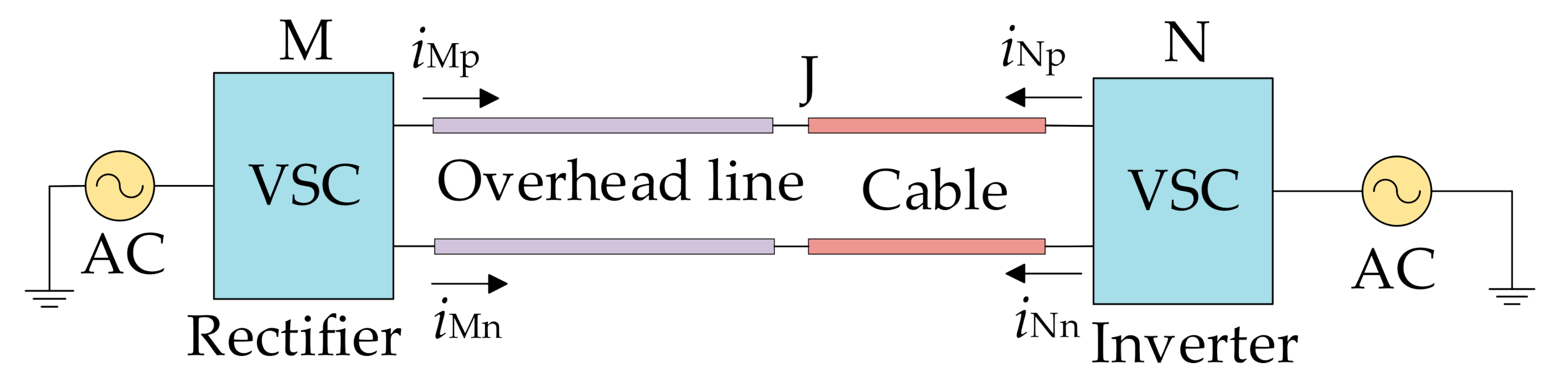
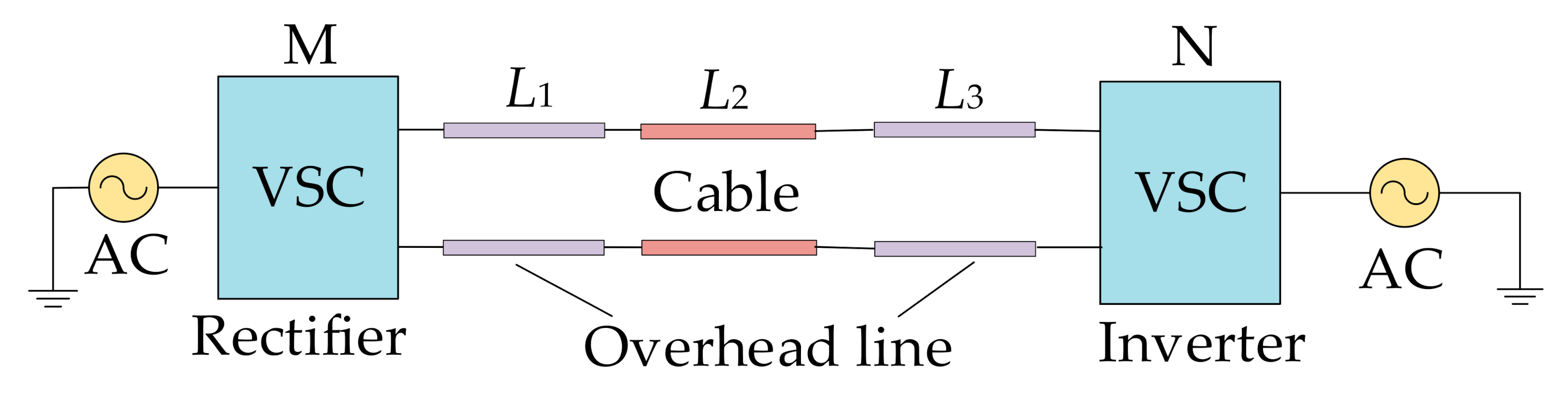
This study mainly investigated the fault location of hybrid transmission lines in a bipolar HVDC system, and its structure is shown in Figure 1. The transmission line on the DC side contains a mix of cables and overhead lines. Their connection point is denoted as J. The DC side close to the power supply and power receiving terminals are denoted as M and N, respectively.
To identify the fault sections, 2D-CNN was considered to classify the characteristic quantities of the fault voltage and current signals at terminal M. Feature engineering is extremely important for identifying fault sections. VMD-TEO was mainly used for this task in this work. A large number of fault signals could be obtained as input samples for CNN considering the combination scenarios of different fault locations, fault types, and transition resistance. The process of obtaining one of these samples is described below.
Bipolar lines have mutual coupling problems, and their parameters have frequency conversion characteristics. Phase-mode analysis is necessary to simplify the calculation process before feature extraction of fault signals. The specific process of phase-mode transformation is expressed as the following formula [31]:
where im0 and im1 are the current or voltage of the ground-mode and aerial-mode traveling wave after decoupling, respectively, and ip and in are the fault current or voltage of the corresponding positive and negative electrodes, respectively.
The principle of VMD-TEO singularity detection was described in detail in References [13,14]. The authors compared this method with WT, HHT, and EMD to prove its excellent detection performance. Feature engineering is mainly through decomposing the fault voltage and current signals at terminal M into several intrinsic mode function (IMF) [32,33] components by VMD and analyzing the first IMF component (IMF1) to obtain Teager energy values (TEVs) by TEO.
To improve the classification effect of 2D-CNN, the TEVs of voltage and current need to be preprocessed using min–max normalization to make them at the interval [0,1], which can be expressed as follows:
where x* is the normalized value, and xmax and xmin are the maximum and minimum values in the sample data, respectively.
The specific HVDC simulation model and related parameter settings are described in detail in Section 4. The sampling frequency was selected to be 100 kHz to improve the accuracy of fault location using the traveling wave method. The time window is 40.96 ms, i.e., 4096 sampling points are found in each time window. Considering the influence of the measurement noise at terminal M, 1% reference signal noise is added to the fault voltage and current of the two poles. Phase-mode transformation is first conducted, and the TEVs of the voltage and current are then calculated and normalized. In this way, a matrix with a size of 2 × 4096 is obtained, which is a 2D-tensor as an input sample. Considering different fault distances, transition resistance, and fault type scenarios, many input samples can be obtained.
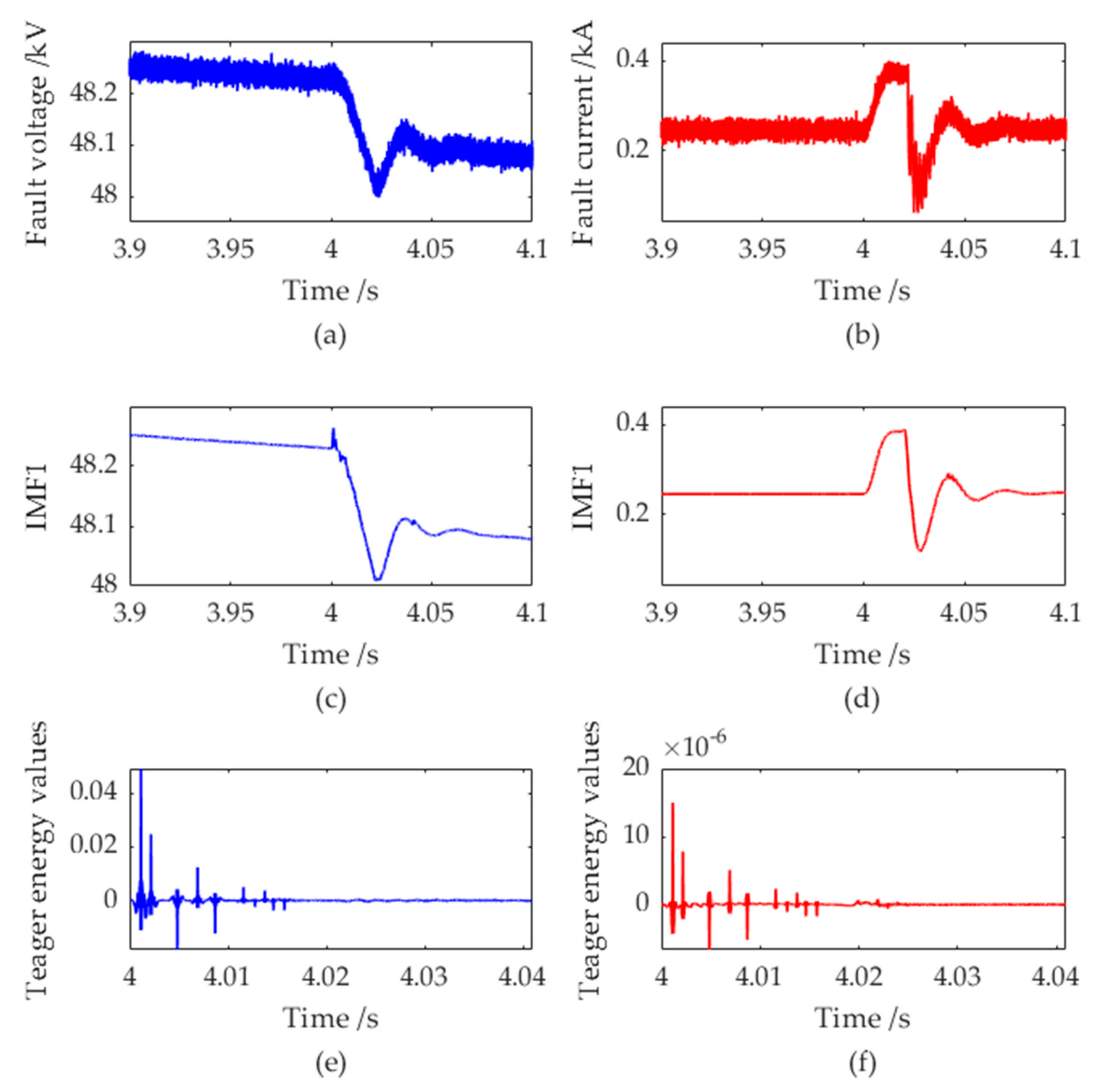
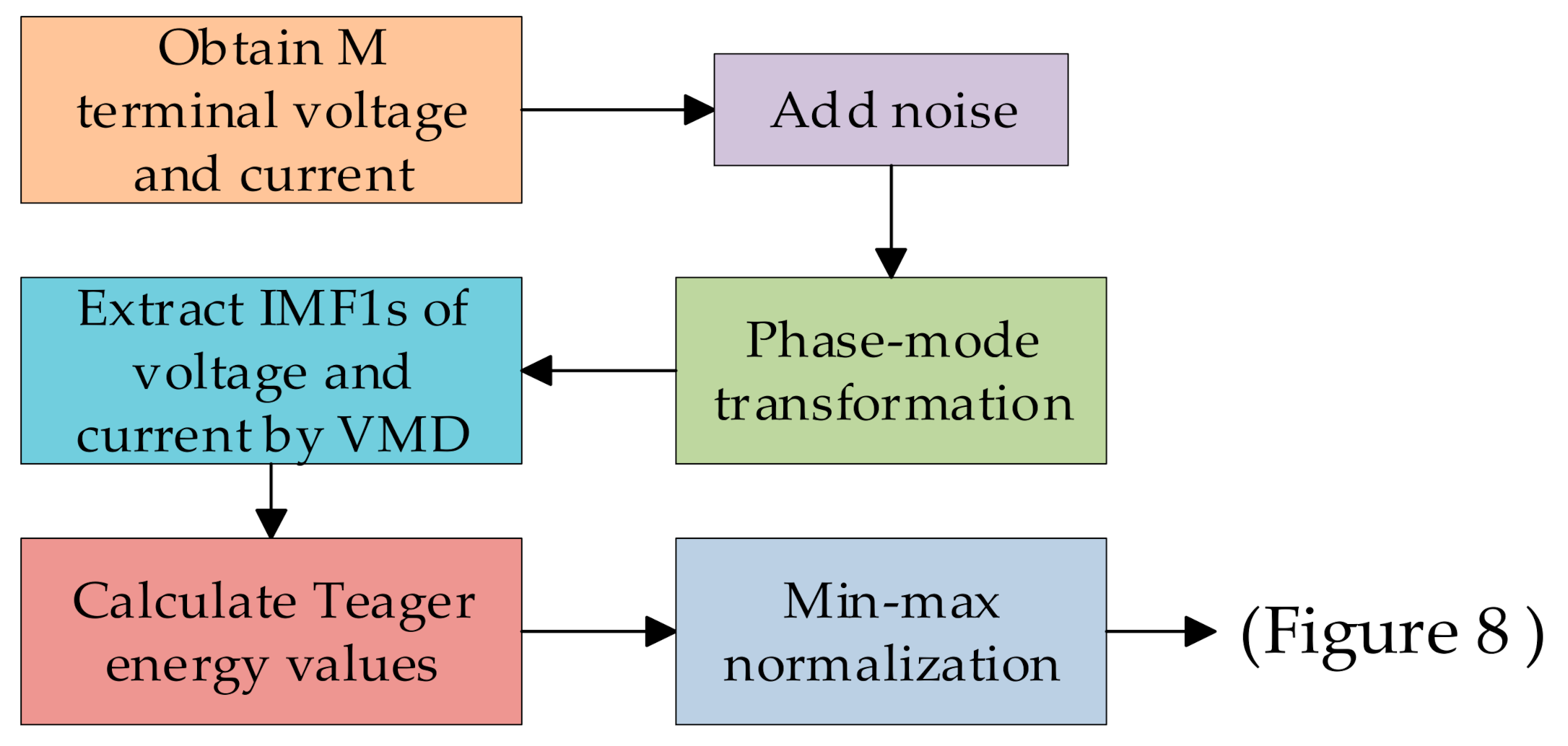
It is assumed that an NG fault occurs at a distance of 350 km from the M terminal, with the transition resistance of 0.03 Ω, the failure time of 4 s, and the duration of 0.02 s. The aerial-mode component of the fault voltage and fault current after noise is added, and the TEVs before normalization is shown in Figure 2. VMD has a good filtering effect because fault signals in Figure 2c,d are much smoother than Figure 2a,b. The calculation of the TEVs based on IMF1 is shown in Figure 2e,f. They have much more high-frequency characteristic signals than Figure 2c,d. Therefore, more useful information of fault signals can be learned after VMD-TEO feature engineering. There is a slight difference in extreme value distribution in addition to the amplitude of TEVs of voltage and current between Figure 2e,f. The TEVs of voltage and current are constructed into 2D-tensor to complement each other with information. The work of classifying fault segments based on this characteristic information needs to be handed over to 2D-CNN for completion. The process of the above feature engineering is shown in Figure 3.
2.2. Fault Segment Identification Based on 2D-CNN
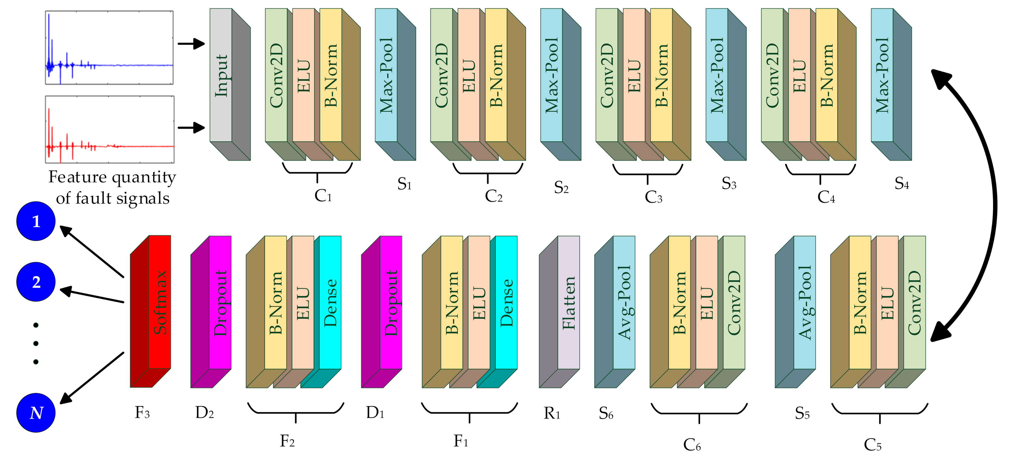
A deep 2D-CNN model was built, as shown in Figure 4. This model consists of 19 layers, including an input layer, six convolutional layers (C1–C6), six pooling layers (S1–S6), a flatten layer (R1), two dense layers (F1, F2), two dropout layers (D1, D2), and a softmax layer (F3). The parameter configuration of each layer in this model is listed in Table 1.
The convolution layer operation can be described as:
where * is the convolution operation, l is the l-th layer in the network, i is the i-th weight in the kernel, j is the j-th kernel, M denotes local feelings, w is the weight of synaptic connections, b is the bias coefficient, z is the result after the convolution operation, xi is the input sample or the feature sample of the previous layer, xj is the output feature sample, and f is the activation function to be selected.
The main chosen activation function of the proposed model is the exponential linear unit (ELU). Compared with the rectified linear unit function, ELU has a negative part. The linear part of ELU can alleviate the vanishing gradient problem, and the negative part can be robust to input changes or noise [34].
The pooling layer can compress and filter the feature samples outputted by the convolution layer, thereby reducing redundant information and network parameters and improving the performance and robustness of the network. The pooling layer operation can be described as:
where down(·) is the subsampling method to be selected, and λ is the weight of the pooling layer.
The fully connected layer can integrate the features of all neurons in the previous layer. The first fully connected layer, such as flatten layer (R1) in Figure 4, has a tiling function that can tile neurons on multiple multidimensional feature samples into 1D vectors. The operation of the fully connected layer can be described as:
where ζ is the weight of the fully connected layer, and f is the ELU activation function.
To prevent overfitting during the learning process, regularization is needed to reduce the generalization error of the model. Batch normalization can prevent gradient dispersion and explosion. The dropout layer can make neurons randomly deactivate with a certain probability, thereby compressing the number of neurons, improving the model learning speed, and effectively reducing overfitting. Here dropout layers (D1, D2) are set as 0.3 and 0.2, respectively.
2.3. Single-Ended Traveling Wave Method for Fault Location
The laws of refraction and reflection of traveling waves on actual HVDC transmission lines vary in different fault segments [7]. The reflected wave head identified on the rectifier side may come from the fault point, the connection point of the hybrid line, or even the bus on the inverter side [23]. Different calculation formulas are adopted in the single-ended traveling wave method when faults occur in different sections [7,23]. When the fault section is located in the first or second halves of the cable, the fault traveling wave propagation is depicted in Figure 5. The lengths of the overhead line and the cable are L1 and L2, respectively. As reported in Reference [16], the wave velocity is a frequency-dependent variable. The traveling wave velocities on the overhead line and the cable are v1(ω) and v2(ω), respectively. Here ω is the frequency when the traveling wave component reaches the rectifier side. Δt is the time difference between the second traveling wave head and the first traveling wave head identified at the M terminal. The distance from the fault point to the M terminal is x, which is the fault location result.
As shown in Figure 5, L1 < x < L1 + L2/2 when the fault occurs at F1, and L1 + L2/2 < x < L1 + L2 when the fault occurs at F2. When the fault point is at F1, the path of the traveling wave is F1-J-F1-J-M, i.e., the second traveling wave head recognized by the M terminal is the reflected wave from the fault point. The fault distance can be calculated using the following formula:
When the fault point is at F2, the path of the traveling wave is F2-N-F2-J-M, i.e., the second traveling wave head recognized by the M terminal is the reflected wave from the opposite bus N. The fault distance can be calculated by the following formula:
There is a complicated nonlinear relationship of the fault distance, the time of the traveling wave reaching the rectifier side and the traveling wave velocity.
3. Fault Location Based on CNN-LSTM
The information on the time of traveling wave reaching the rectifier side and wave velocity can be obtained through combining the fault signal after feature engineering with the corresponding fault distance. A nonlinear relationship is found between these feature quantities and fault distance. These feature quantities have time correlation since it can be regarded as time series. LSTM can be used for the regression prediction of fault distances. The complete fault location process of CNN-LSTM is shown in Figure 6. The fault voltage and current are obtained at the M terminal. High-frequency components (TEVs) of the fault traveling wave are extracted by phase-mode transformation and VMD-TEO. Then TEVs are constructed into a 2D-tensor as an input of 2D-CNN. Finally, the fault location is performed through the trained LSTM model.
3.1. Theoretical Background of LSTM
An LSTM network is an improved temporal recurrent neural network. The introduction of a forgetting gate solves the problem of gradient disappearance during training, enabling LSTM to learn the long-term and short-term dependence information of time series [18,30]. Its network basic unit is shown in Figure 7.
The basic unit of LSTM contains forget, input, and output gates. Input xt in the forget gate, state memory unit St−1, and intermediate output ht−1 together determine the forgotten part of the state memory unit. xt in the input gate is determined by the sigmoid and tanh functions to jointly determine the vector retained in the state memory unit. Intermediate output ht is jointly determined by the updated St and ot. The calculation formulas in these processes are expressed as follows:
where ft, it, gt, ot, ht, and St are the states of the forget gate, input gate, input node, output gate, intermediate output, and state unit, respectively, Wfx, Wfh, Wix, Wih, Wgx, Wgh, Wox, and Woh are the matrix weights of the corresponding gate multiplied by input xt and intermediate output ht−1, bf, bi, bg, and bo are the bias terms of the corresponding gate. ☉ is the bitwise multiplication of the elements in the vector. σ is the sigmoid function, and φ is the tanh function.
3.2. CNN-LSTM Hybrid Model for Fault Location
A CNN-LSTM hybrid model showed in Figure 8 is built based on the previous 2D-CNN structure. The model 2D-CNN in the left half as a classifier completes the task of identifying fault segments, and the model LSTM in the right half as a regressor completes the task of precise fault location. The fault segment with the highest probability output from the softmax function is selected as the current fault segment. The feature information output by the flatten layer (R1) in 2D-CNN and the probability information of the fault segment are calculated by the regressor. The experimental results demonstrate that six LSTM layers should be used in the CNN-LSTM network, and each LSTM layer contains 64 neurons. The dense layer (F4) uses a neuron. The loss function is mean squared error, and the optimizer is Adam. The proposed hybrid network model can intelligently integrate information from different fault sections and corresponding fault distances, and continuously optimize and update network parameters to make it close to ideal.
With the development of modern data acquisition technology and deep learning technology, the proposed method is feasible for engineering applications. A high-precision and adjustable sampling frequency transient recorder is installed on the M terminal to obtain a large number of fault sample data. The operation of the proposed method can be accelerated by parallelizing on graphical processing units or tensor processing units. After the proposed model is trained, it can be used repeatedly for fault location, and the speed is calculated in milliseconds. Circuit breakers in HVDC systems, which is a key element to interrupt and clear the faults [35]. The fault location speed of the proposed method can meet the operating time requirements of an actual circuit breaker. Feature engineering is performed in MATLAB 2019a. The model training and testing are carried out on the Python3.7 Keras framework.
4. Simulation Results and Analysis
4.1. Simulation Model and Related Parameters
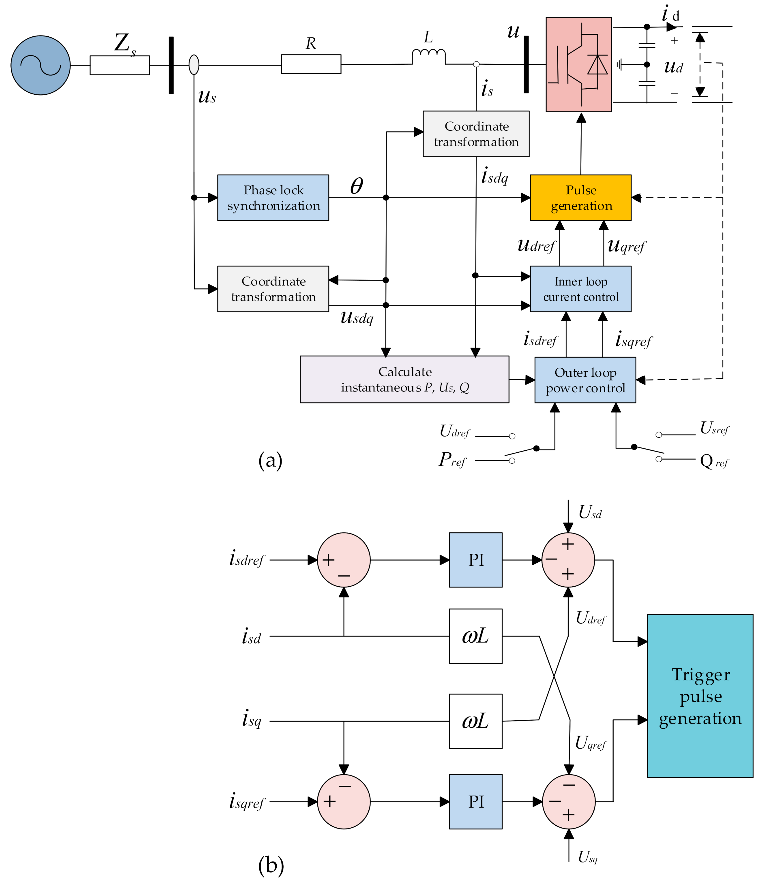
The voltage source converter (VSC)-HVDC transmission system with mixed lines in Figure 1 is constructed on the power system simulation software PSCAD/EMTDC. The model proposed in Reference [14] was used in this study. Its structure and related parameter settings remained constant. In this paper, a bipolar DC transmission line power and a current double closed-loop proportional–integral (PI) control were adopted. The VSC overall control system structure is shown in Figure 9a comprising the inner loop current controller, outer loop power regulator, phase lock synchronization, trigger pulse generation, and other components, in which the inner loop current controller is used to directly control the AC side current waveform and the phase of the converter is applied to rapidly track the reference current. The outer loop power control is based on the control objectives of the system, i.e., DC voltage, active power, fixed frequency, reactive power, constant AC voltage, and other control objectives. The outer loop control mode of the M-side keeps constant active power control and constant reactive power control, whereas the outer loop control mode of the N-side is constant DC voltage and constant reactive power control. The inner loop controllers of the M-side and N-side are identical, and their controller structure is demonstrated in Figure 9b.
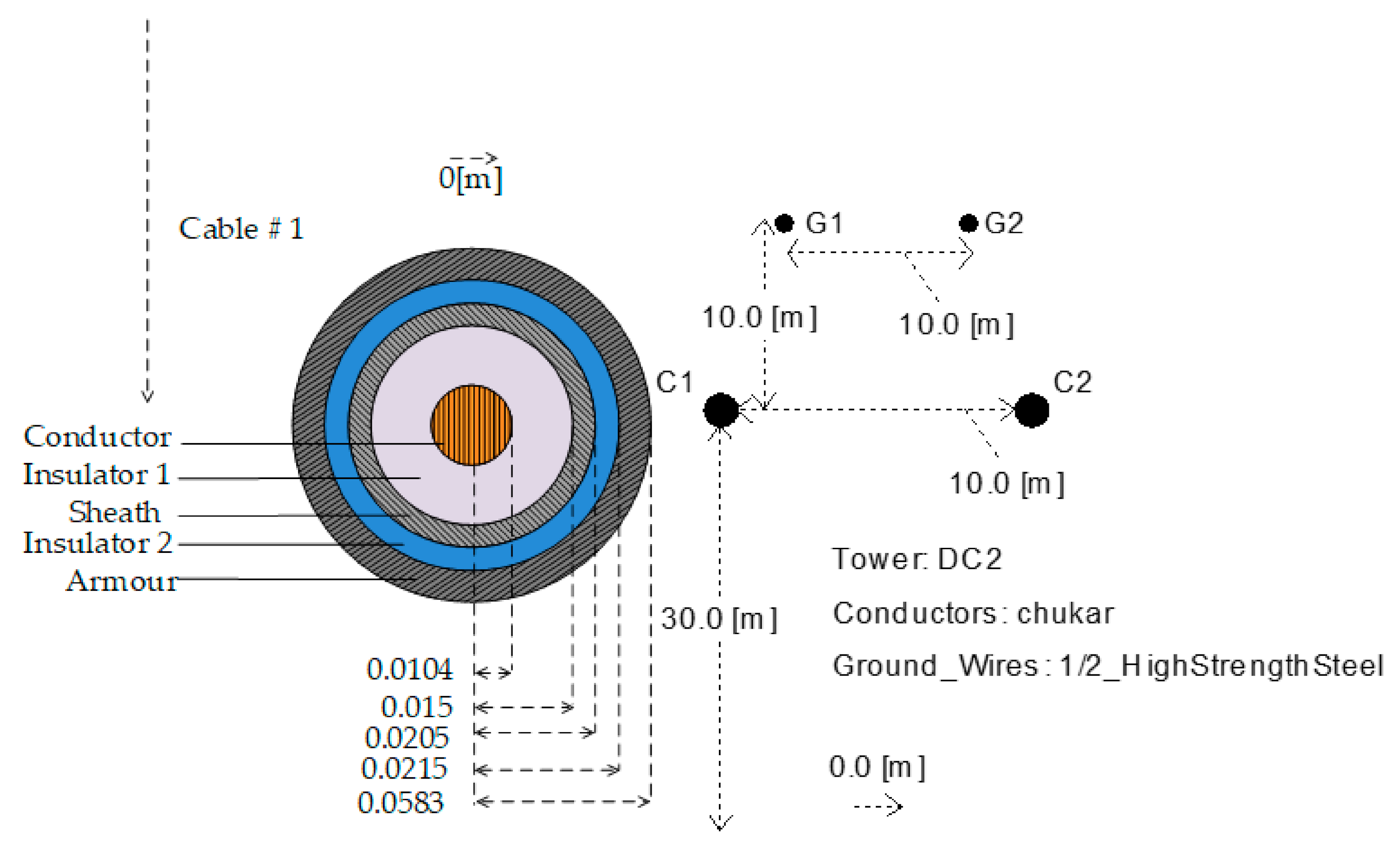
The M-side system was modeled by a three-phase voltage source with the following main parameters; the line voltage of 110 kV, system impedance of 1.7 Ω, transformer Yn/Δ link capacity of 25 MVA, winding voltage of 110 kV/25 kV, leakage resistance of 0.2 pu, phase reactor of 0.053 H, and equivalent resistance of 0.8 Ω. The N-side system was simulated as an infinite system by a three-phase voltage source with the following main parameters; the system impedance of 0 Ω, line voltage of 110 kV, transformer Yn/Δ link, capacity of 20 MVA, winding voltage of 110 kV/25 kV, leakage resistance of 0.1 pu, phase reactor of 0.053 H, and equivalent resistance 0.6 Ω. Modeling cables and overhead lines using the frequency dependent (phase) approach are shown in Figure 10. The resistance, sheath resistivity, and armor resistivity of the cable are 1.72 × 10⁻⁸, 2.2 × 10⁻⁷, and 1.8 × 10⁻⁷ Ω·m, respectively. The relative dielectric constant of the insulator is 2.5 with length of 200 km. The resistance, GMR, and length of the overhead wire are 0.03206 Ω/km, 0.0122834 m, and 300 km, respectively.
4.2. Experimental Result of Traveling Wave Method
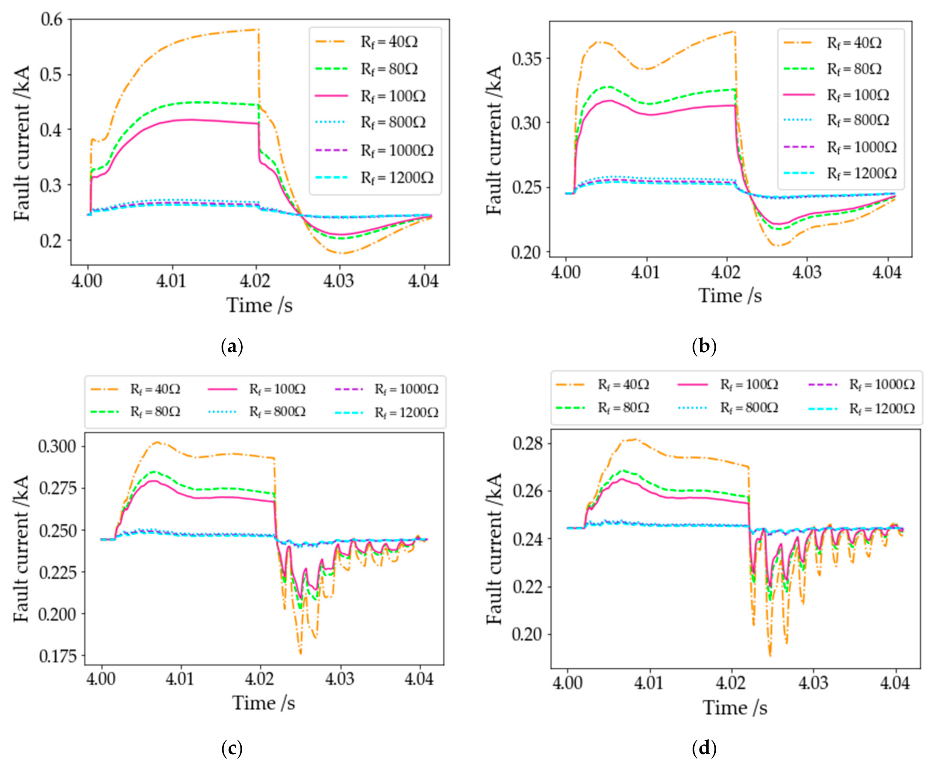
The fault resistance value used to distinguish HIF and LIF is related to specific HVDC system parameters. This research is mainly based on the change of the fault current. An assumption is that a positive ground (PG) fault occurs at a distance of 50, 150, 300 and 400 km from the M terminal. When the transition resistance Rf changes, the aerial-mode component of the fault current is shown in Figure 11. When Rf is less than 100 Ω, the fault current amplitude is larger and its variety is more obvious than that when Rf is between 800 and 1200 Ω. Through this analysis, it can be seen that the fault resistance of LIF and HIF ([0, 100 Ω] and [800 Ω, 1200 Ω], respectively) is one of the reasonable circumstances.
As depicted in Reference [7], the hybrid line was divided into four fault segments, and SVM was used to identify these sections. In this work, 2D-CNN was used to achieve this aim. A large number of CNN input samples can be obtained through different fault scenarios. The sampling frequency and time window are 100 kHz and 40.96 ms, respectively. A total of 4096 sampling points is found in each time window. Three fault conditions include PG, NG, and short between positive and negative (PN). The maximum transition resistance is 100 Ω with LIF considered. The performance of the proposed method is evaluated for various fault scenarios under different system conditions. The simulations are conducted with the following values or types:
- (1)
- The change step size of the fault distance is taken as 1 km.
- (2)
- Transition resistance Rf = 0.0001%, 1%, 2%, 3% … 100% of the maximum transition resistance.
- (3)
- Fault types include PG, NG, and PN.
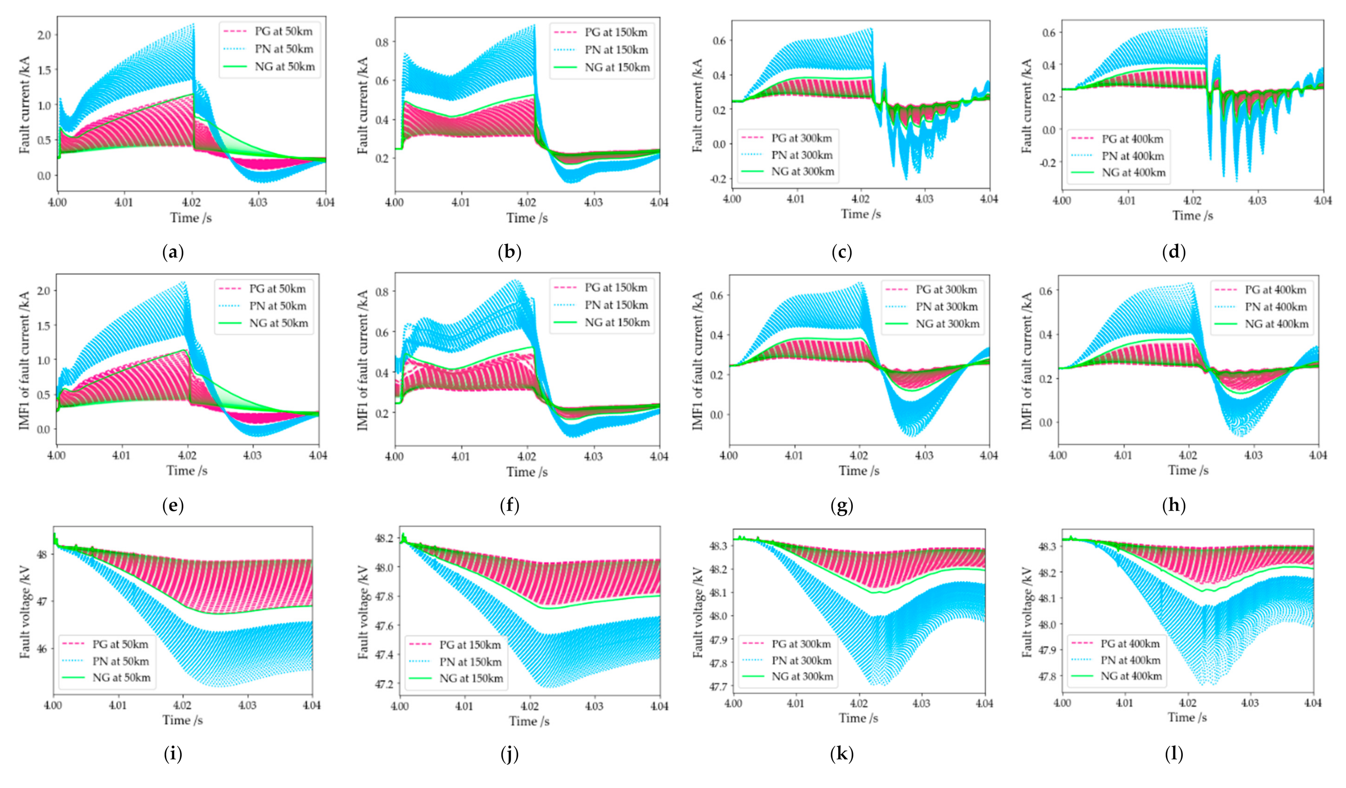
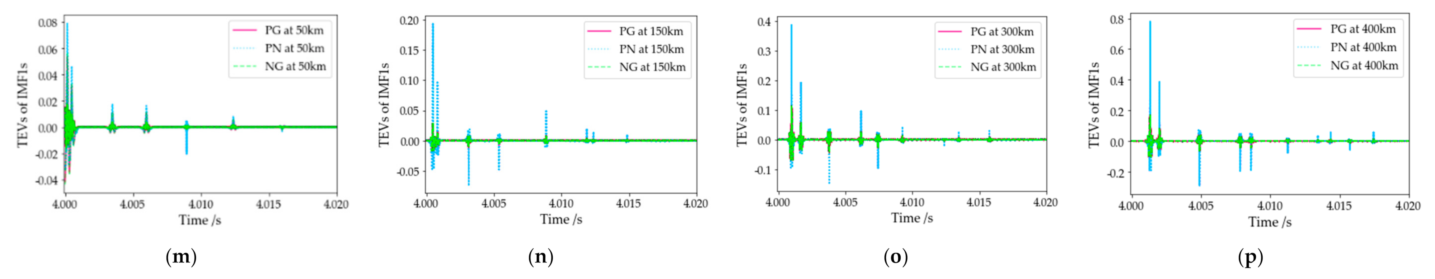
A total of 151,197 different cases were simulated, and 1% reference signal noise was considered. After performing feature engineering by VMD-TEO on all simulation results, 151,197 input samples can be obtained as input samples for CNN. Due to the large number of samples, only samples with fault points located at 50, 150, 300 and 400 km are displayed in Figure 12. There are 101 samples in each of the three fault scenarios corresponding to each fault distance. In different fault sections, changes of the voltage and current are different as shown in Figure 12a–d,i–l. After the fault signals are processed by VMD, the high frequency components, which are IMFs, of the fault traveling wave can be obtained as shown in Figure 12e–h. Yet, the characteristics of these components are not obvious. If they are directly used in deep learning for fault segment identification and fault location, the number of training samples and the complexity of the neural network will greatly increase. However, after VMD-TEO feature engineering is performed on the fault signals, as shown in Figure 12m–p, the information of these high-frequency components will become clearer. Therefore, this feature engineering is conducive to the learning of the CNN-LSTM network. The extreme point positions of the high-frequency components (TEVs) are related to the fault distances, and are less affected by the fault types. Simultaneously, the amplitude of these components and the polarity of the extreme values varied with the fault distances. TEVs of IMFs are feasible as input to the CNN-LSTM model.
Randomly take 80% of the total sample as training data and the remaining samples as test data. One-hot coding is performed for the four fault sections, i.e., the first and second halves of the overhead line and cable are encoded as [1,0,0,0], [0,1,0,0], [0,0,1,0], and [0,0,0,1].
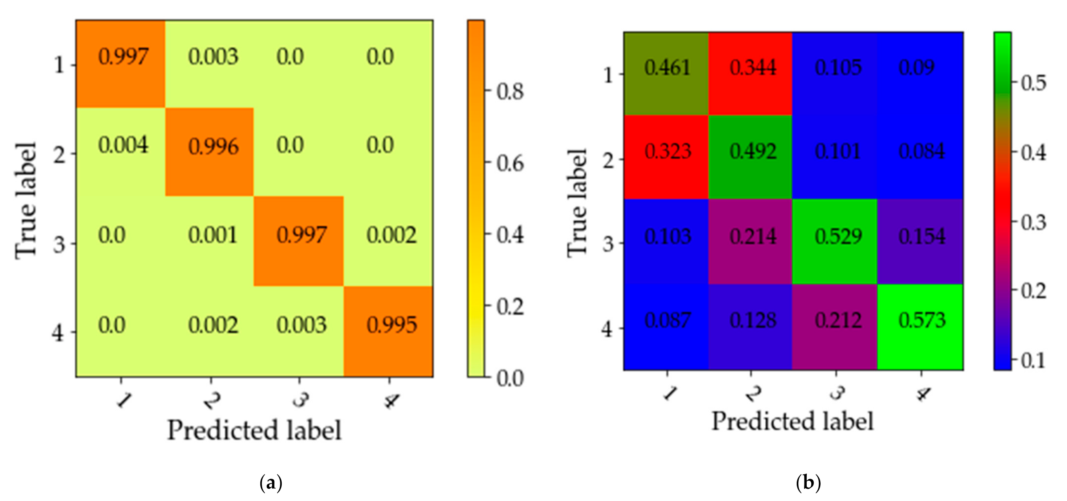
When LIF occurs, the test results are represented by a normalized confusion matrix, as shown in Figure 13a. The recognition effect of the four fault sections is excellent with an accuracy rate over 99.5% in Figure 13a. Under consideration of HIF, the value range of fault resistance is [800 Ω, 1200 Ω]. In this interval, the change step of fault resistance is 4 Ω. The other failure scenario settings are the same as above, and a total of 151,197 different cases can also be obtained. The normalized confusion matrix of the test results in this case is shown in Figure 13b. The recognition effect of the four fault sections is extremely poor, the lowest and fault recognition rates are 46.1% and 57.3%, respectively. The classification method of the four fault sections can only be used in the case of LIF and is not applicable to the case of HIF.
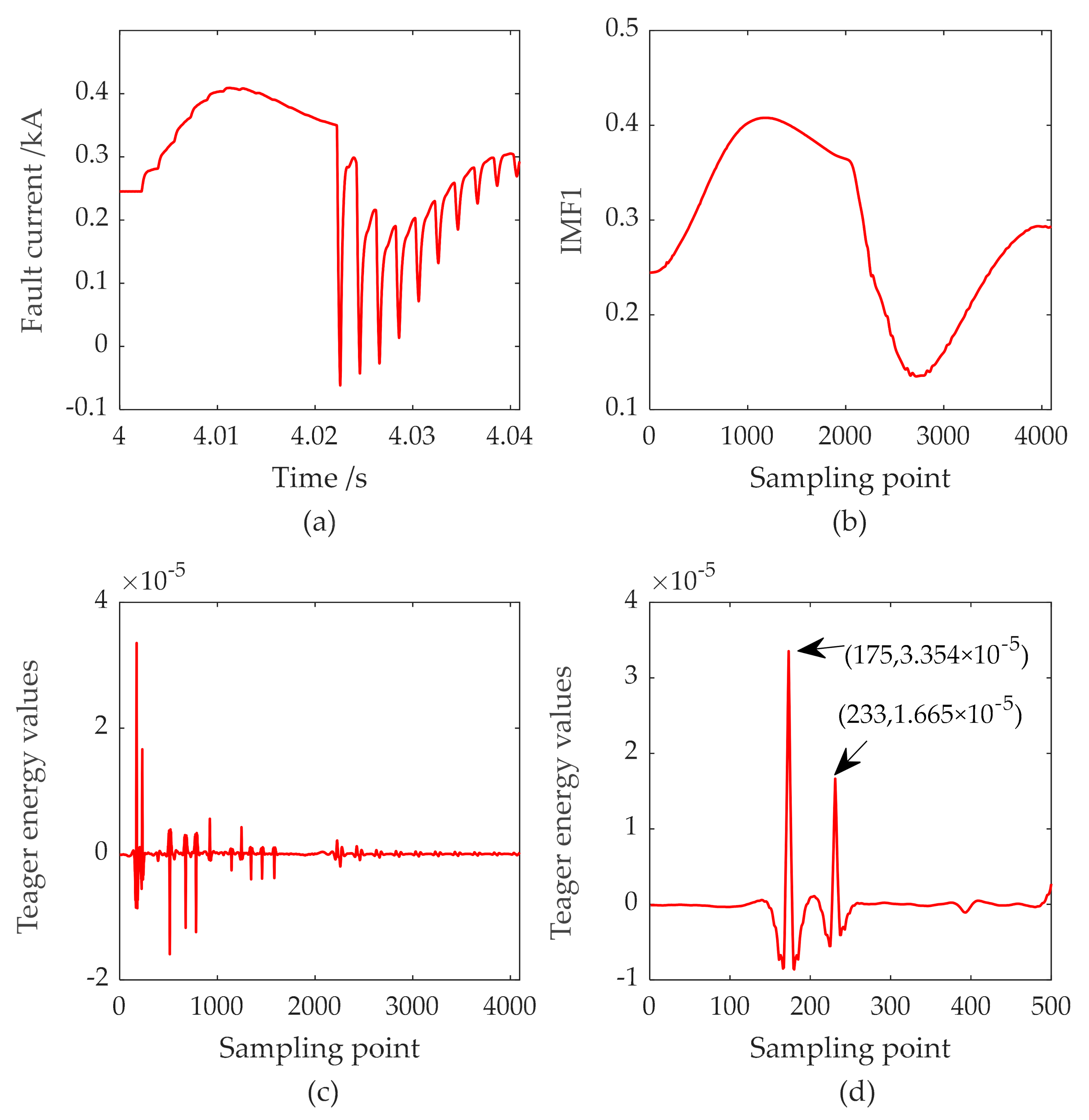
Assuming that PN LIF occurs at a distance of 450 km from the M terminal, the transition resistance is 10 Ω, the time of failure is 4 s, the duration is 0.02 s, and the fault section can be correctly identified. The fault current signal at the M terminal and the result of the singularity detection using the VMD-TEO are recorded in Figure 14. The IMF1 obtained by VMD can reflect the essential characteristics of the fault signal. After calculating the TEV of IMF1, evident extreme points are obtained. The positions of these extreme points can reflect the positions of singular points of the signal. In accordance with the previous analysis, the first two extreme points are the traveling wave initial wave head and the opposite wave bus head, respectively. The fault distance can be calculated using Formula (7), where td1 = 4.00175 s, td2 = 4.00233 s. According to the theoretical analysis [7,14], it is assumed that the parameters of the aerial-mode component do not change much, and the influence of frequency on the traveling wave velocity is ignored. Since the HVDC model and parameters in this study are exactly the same as that described in Reference [14], the fixed aerial-mode traveling wave velocities in Reference [14] are used for calculation, where v1 = 293,997.1102 km/s, v2 = 196,333.3333 km/s. The theoretical value of fault distance is 443.063 km, the error distance of fault distance is 6.937 km, and the error percentage is 1.54%. This error does not meet the actual engineering requirements. The possible reason of the error is that fixed traveling wave velocities are adopted while ignoring their frequency variation characteristics.
4.3. Experimental Result of CNN-LSTM
Several shortcomings are found in the previous fault location analysis of the traveling wave method. The connection points of the fault sections are not considered. The effect of identifying HIL is extremely poor. Many overlapping fault sections are considered to solve these problems.
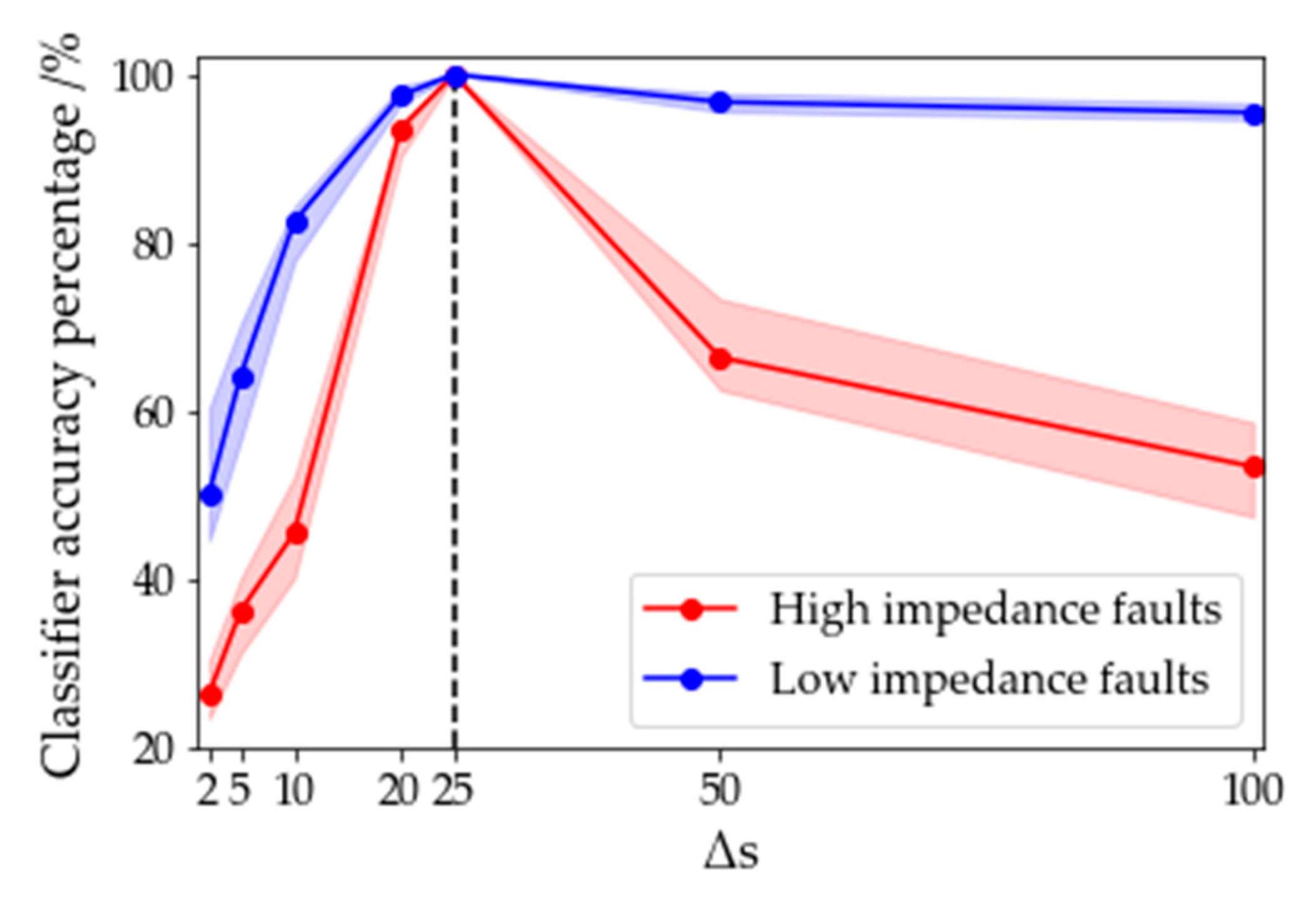
The length of the mixed line and the overlap of the fault sections are considered as the length of the sample (Ls) and its offset (Δs), respectively. When Δs is large, the number of categories (N) of the fault sections is small. When N is small, the recognition rate for HIF is low. When N is large, the data amount and learning effect of CNN-LSTM are affected. Therefore, the selection of appropriate Δs is very important for accurate fault location.
The length of the mixed line is 500 km, and the interval of Ls is [0, 500]. When Δs = 100, N = 4, the fault sections are [0, 200], [100, 300], [200, 400], and [300, 500]. When Δs = 50, N = 9, the fault sections are [0, 100], [50, 150],…, and [400, 500]. When Δs = 25, N = 19, the fault sections are [0, 50], [25, 75],…, and [450, 500]. Δs is changed, and the classification experiments of HIF and LIF are performed again. With the change in Δs (Δs = 2, 5, 10, 20, 25, and 100), the accuracy percentage of the 2D-CNN classifier is shown in Figure 15. The width of the ribbon in Figure 15 reflects the accuracy range of each fault segment identification, where the edges of the ribbon reflect the maximum and minimum accuracy, and the solid line reflects the average accuracy. When Δs = 25, i.e., N = 19, the classification effect of HIF and LIF is best with accuracies of 99.98% and 99.99%, respectively.
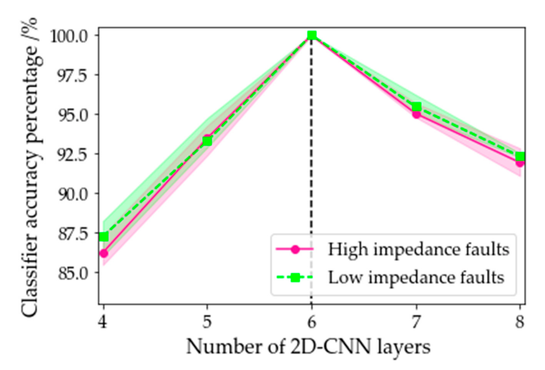
The number of 2D-CNN layers can affect the classification effect of CNN-LSTM. Take the number of CNN layers as 4, 5, ..., 8 and N = 19 for experimental tests, and the results are shown in Figure 16, which is similar to Figure 15. When the number of 2D-CNN layers changes, the accuracy range of the classification in 19 fault sections includes the maximum, minimum, and average values. Properly increasing the number of 2D-CNN layers can improve the classification ability of the model. However, the accuracy of training decreases when the number of 2D-CNN layers exceeds six layers, indicating that the model is overlearning. When the number of 2D-CNN layers is 6, the accuracy of the classifier in the 19 fault sections is close to 100%, and the variation range is the smallest. Therefore, the 6-layer 2D-CNN model is reasonable as a classifier.
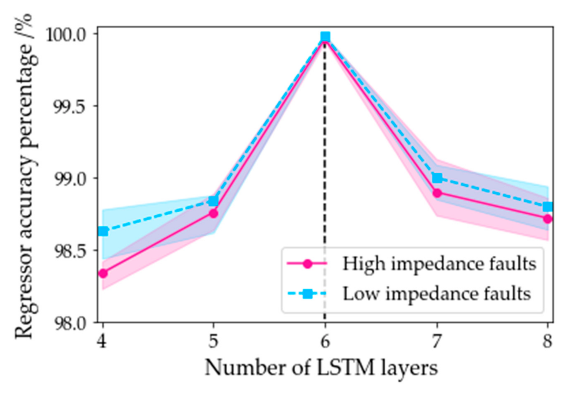
The influence of the number of LSTM layers on the regression effect of CNN-LSTM is also considered. Take the number of LSTM layers as 4, 5, ..., 8 and N = 19 for experimental tests, and the results are shown in Figure 17, which is similar to Figure 15 and Figure 16. When the number of LSTM layers changes, the accuracy range of the regression prediction in each fault section includes the maximum, minimum, and average. The accuracy calculation sets a fault distance tolerance of ±0.5%, thereby meeting the actual engineering requirements. The predicted values of multiple samples for each fault distance are averaged. The predicted value is recorded as accurate when the average is within the fault distance tolerance. When the number of LSTM layers is more than or less than six, the accuracy of the regressor is not as good as that of the six-layer LSTM. The predicted fault distances are highly accurate at each fault section.
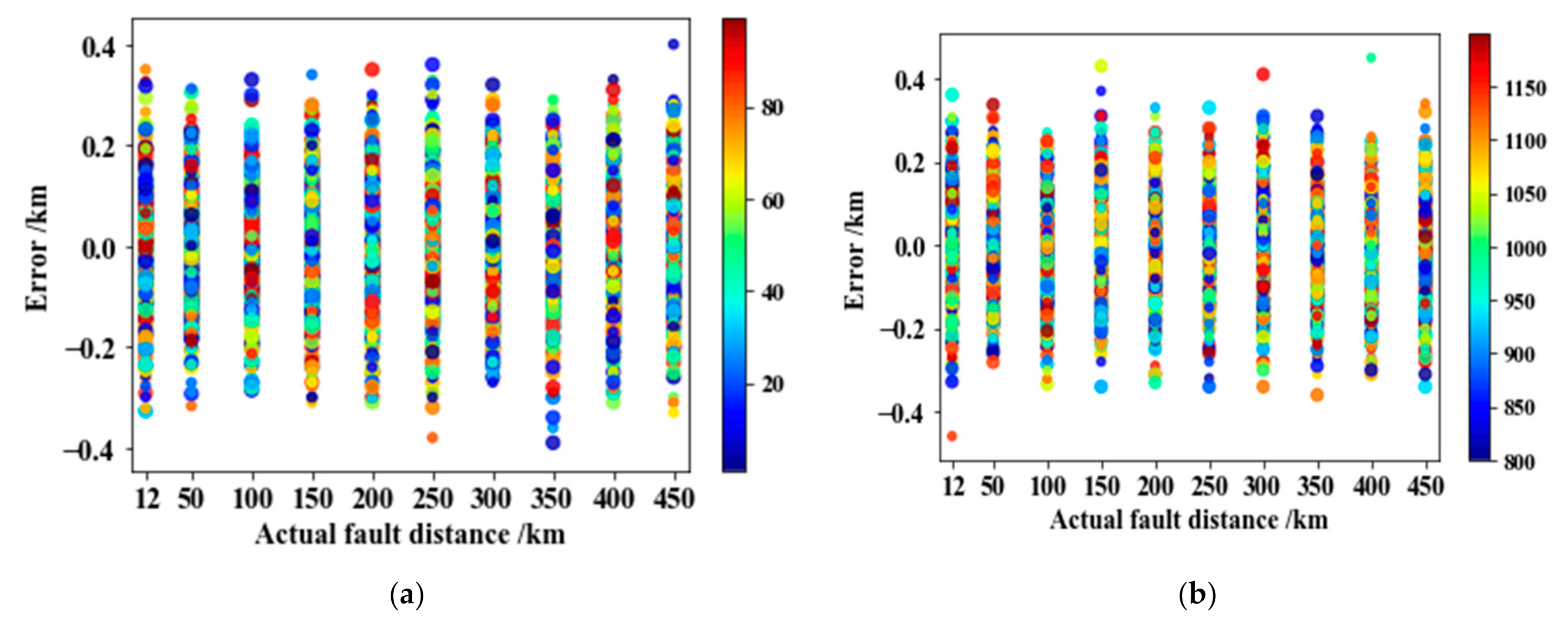
The CNN-LSTM network with six LSTM layers was chosen for the test. The 500 sets of data with a fault distance of 12, 50, ..., and 450 km are randomly taken for experiments. Regression is used to predict the fault distance by CNN-LSTM and calculate the error. The experimental results of LIF and HIF are shown in Figure 18a,b, respectively. The color of the circle in the scatter plot reflects the value of fault resistance ([0.01 Ω, 100 Ω], [800 Ω, 1200 Ω]), and the size of the circle reflects the fault types (PG, NG, PN). The vertical axis of the scatter plot is the fault distance error without considering the tolerance, i.e., the difference between the actual fault distance and its predicted value. The fault error values of LIF and HIF are approximately concentrated in the range of −0.4 to 0.4 km. The proposed method has small fault location error, and is less affected by fault resistances and fault types.
4.4. Influence of Sampling Frequency
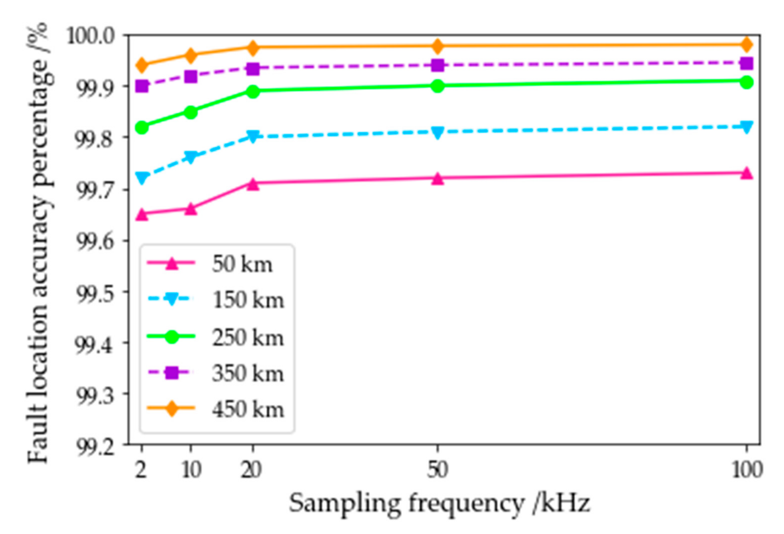
The traveling wave method requires the measurement device to use a high sampling frequency, which is disadvantageous for practical engineering applications. To illustrate the effect of sampling frequency on the experimental results of CNN-LSTM, the sampling frequencies are taken as 100, 50, 20, 10, and 2 kHz. Regressive prediction is performed on 1000 groups of data with fault distances of 50, 150, 250, 350, and 450 km. The accuracy percentage of the fault location is obtained as follows:
where yact is the actual fault distance, ypred is the predicted fault distance, N1 and N2 are the number of test samples for HIF and LIF, respectively, and N1 = N2 = 500.
The accuracy of fault location at different sampling frequencies is shown in Figure 19. When sampling frequency is between 20 and 100 kHz, the change in the accuracy of CNN-LSTM fault prediction is relatively stable. Therefore, the method requires lower sampling frequency than the traveling wave method.
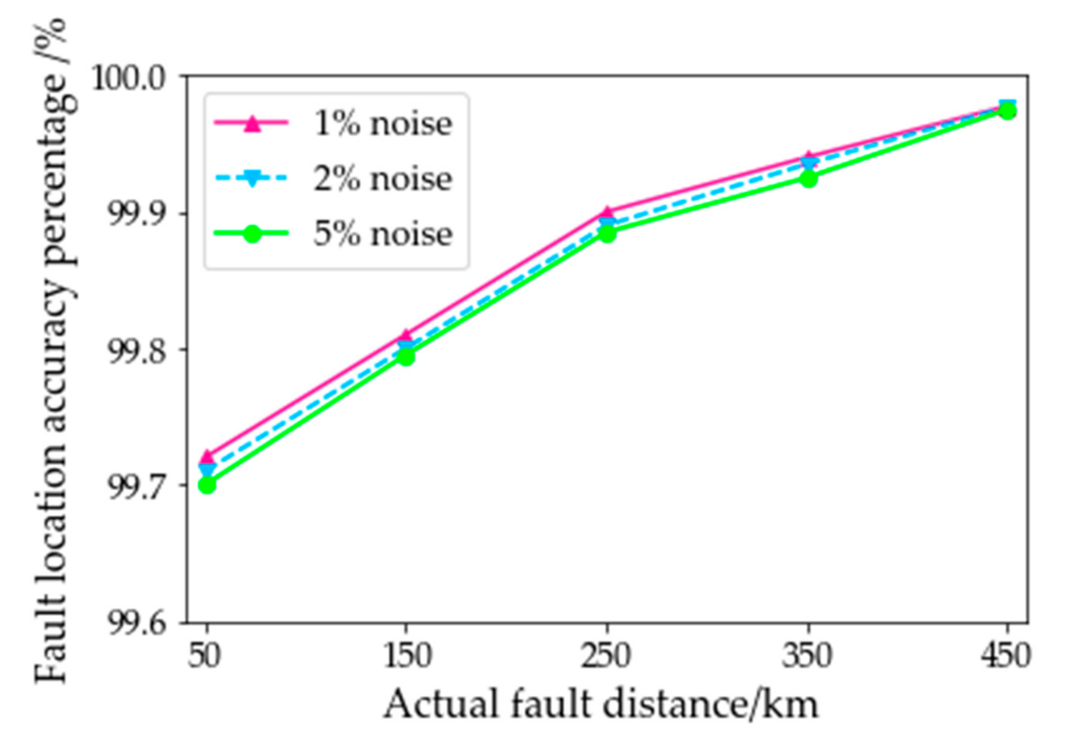
4.5. Influence of Noise
In the previous experimental analysis, the influence of measurement noise at the M terminal is considered, and 1% reference signal noise is added. Considering the effect of load changes during the actual operation of the HVDC system, 2% and 5% reference signal noises are added to the voltage and current signals at the M terminal. Similar to the process of analyzing the effect of sampling frequency on the accuracy of fault location, 1%, 2%, and 5% reference signal noises are added for fault prediction, and the sampling frequency is 50 kHz. The accuracy of fault location testing at different noise levels is shown in Figure 20. The effect of fault location is slightly affected by different levels of noise environment. The roles of VMD and CNN make the CNN-LSTM fault location method robust to noise.
4.6. Comparison of Other Methods
This study reasonably reduces the sampling frequency from 100 to 50 kHz to test HIF. In order to achieve a fair comparative test, the following methods adopt the same training and testing samples. Different feature engineering methods such as WT, HHT and VMD-TEO in this study are considered for experimental comparison. The experimental results are displayed in Table 2. The results by CNN-LSTM in the table are the average of 500 sets of test data. Since the data in the table are average values, it may happen that the test results cannot meet the allowable error range of actual engineering applications. Different feature engineering methods have a great influence on the accuracy of fault location, which can be seen in Table 2. It is verified here that the VMD-TEO method mentioned in our previous work [14] is superior to WT and HHT in terms of singularity recognition and robustness. The error in WT may be caused by the difficulty in using WT to select the basic functions and decomposition scales, and the error source of HHT may be a modal aliasing phenomenon in the EMD decomposition process.
In order to facilitate the comparison of experiments, the 2D-CNN classifier structure of the left half of the proposed model remains unchanged. Other regression algorithms such as 1D-CNN, GRU, and Bi-GRU are used to replace the regressor in the right half of the proposed hybrid model. The experimental results by different regression methods are listed in Table 3. The comparison of the test effects of these three deep learning methods shows that the effect of LSTM in the regressor is significantly better than that of 1D-CNN, GRU, and Bi-GRU. The average error interval of CNN-LSTM, 1D-CNN, GRU and Bi-GRU are in [0.137, 0.265 km], [4.104, 5.213 km], [1.104, 1.333 km], and [1.821, 2.721 km], respectively. The fluctuation range of the error value of CNN-LSTM fault location is within the range of error tolerance value of actual engineering application. 1D-CNN has the worst experimental accuracy because its ability to learn the time correlation of fault signals is not as good as GRU, Bi-GRU and LSTM. GRU is a simplified model of the LSTM structure, which reduces the amount of calculation. However, reducing the model parameters may not guarantee that the regression effect is better than LSTM. Bi-GRU is that GRU learns the time series from the forward and reverse directions. The reason that the experimental accuracy of Bi-GRU is not as good as that of GRU and LSTM is that all regression prediction capabilities must come from the forward learning of the Bi-GRU network, and the reverse learning performs poorly on this task.
4.7. Other HVDC Model
In order to verify the feasibility of the proposed method in the other HVDC model, the topology in Figure 1 is changed to the form in Figure 21. Here L1 and L3 are overhead lines with a length of 150 km, and L2 is a cable with a length of 150 km. The CNN-LSTM model is retrained according to the previous program, and 10 samples are randomly selected for testing, as shown in Table 4. The error interval of the proposed method is in [0.249, 0.379 km]. This error range also meets engineering needs. By the analysis of Table 4, it can be concluded that this fault location method has higher accuracy when considering different HVDC topologies, and is also rarely affected by fault types and fault resistance.
5. Conclusions
A deep CNN-LSTM method was proposed to locate the fault in HVDC systems with mixed cables and overhead lines. In the case of LIF and HIF, this method has high fault location accuracy with the effects of fault types, noise, sampling frequency, and different HVDC topologies in consideration.
VMD-TEO is used in feature engineering to improve the learning effect of the model. Experimental results prove that this method is superior to WT and HHT in feature extraction. This single-ended intelligent method transforms the problem of this research into two tasks: fault section identification by a 2D-CNN classifier and fault precise location by an LSTM regressor. Simultaneously, the regressor integrates the fault section information in the classifier, and finally completes the fault location task. Other deep learning methods such as 1D-CNN, GRU and Bi-GRU replace LSTM in the regressor as an experimental comparison. Experimental results show that the fault location accuracy of LSTM is better than other methods.
Regarding the choice of the deep learning algorithm, it needs to be based on actual data. Although it is mentioned in References [26,27] that GRU and Bi-GRU are optimizations of LSTM, the results of this experimental data analysis cannot prove such a conclusion. GRU simplifies the structure of LSTM and accelerates operations, but its learning effect is not as good as LSTM. Bi-GRU learns the characteristics of time series from both forward and reverse directions, but learning from the reverse direction is far worse than from the forward direction. The experimental results of Bi-GRU are not as good as LSTM, and even worse than GRU.
Author Contributions
Conceptualization, methodology, software, validation, formal analysis, investigation, resources, L.W. and Y.H.; data curation, writing—original draft preparation, L.W.; writing—review and editing, L.L.; visualization, L.L. All authors have read and agreed to the published version of the manuscript.
Funding
This research was supported by the National Natural Science Foundation of China (Grant No. 51977153, 51977161, and 51577046), the State Key Program of National Natural Science Foundation of China (Grant No. 51637004), the national key research and development plan “important scientific instruments and equipment development” of China (Grant No. 2016YFF0102200), the Equipment research project in advance of China (Grant No. 41402040301).
Informed Consent Statement
Informed consent was obtained from all subjects involved in the study.
Data Availability Statement
The raw/processed data required to reproduce these findings cannot be shared at this time as the data also forms part of an ongoing study.
Conflicts of Interest
The authors declare no conflict of interest.
Abbreviations
| HVDC | High voltage direct current |
| CNN | Convolutional neural network |
| LSTM | Long short-term memory |
| VMD | Variational mode decomposition |
| TEO | Teager energy operator |
| WT | Wavelet transform |
| HHT | Hilbert–Huang transform |
| VMD-TEO | Variational mode decomposition–Teager energy operator |
| EMD | Empirical mode decomposition |
| LIF | Low impedance fault |
| HIF | High impedance fault |
| RNN | Recurrent neural network |
| GRU | Gated recurrent unit |
| Bi-GRU | Bidirectional gated recurrent unit |
| IMF | Intrinsic mode function |
| IMF1 | The first intrinsic mode function component |
| TEV | Teager energy value |
| VSC | Voltage source converter |
| NG | Negative ground |
| ELU | Exponential linear unit |
| PG | Positive ground |
| PN | Positive and negative |
References
- Nanayakkara, O.M.K.K.; Rajapakse, A.D.; Wachal, R. Location of DC line faults in conventional HVDC systems with segments of cables and overhead lines using terminal measurements. IEEE Trans. Power Deliv. 2012, 27, 279–288. [Google Scholar] [CrossRef]
- Chen, K.; Hu, J.; Zhang, Y.; Yu, Z.; He, J. Fault location in power distribution systems via deep graph convolutional networks. IEEE J. Sel. Areas Commun. 2020, 38, 119–131. [Google Scholar] [CrossRef] [Green Version]
- Bains, T.P.S.; Sidhu, T.S.; Xu, Z.H.; Voloh, I.; Zadeh, M.R.D. Impedance-based fault location algorithm for ground faults in series-capacitor-compensated transmission lines. IEEE Trans. Power Deliv. 2018, 33, 189–199. [Google Scholar] [CrossRef]
- Kezunovic, M. Smart Fault Location for Smart Grids. IEEE Trans. Smart Grid 2011, 2, 11–22. [Google Scholar] [CrossRef]
- Shu, H.C.; Han, Y.M.; Huang, R.; Tang, Y.T.; Cao, P.L.; Yang, B.; Zhang, Y. Fault Model and Travelling Wave Matching Based Single Terminal Fault Location Algorithm for T-Connection Transmission Line: A Yunnan Power Grid Study. Energies 2020, 13, 1506. [Google Scholar] [CrossRef] [Green Version]
- Lin, S.; He, Z.; Li, X. Travelling wave time-frequency characteristic-based fault location method for transmission lines. IET Gener. Transm. Distrib. 2012, 6, 764–772. [Google Scholar] [CrossRef]
- Livani, H.; Evrenosoglu, C.Y. A single-ended fault location method for segmented HVDC transmission line. Electr. Power Syst. Res. 2014, 107, 190–198. [Google Scholar] [CrossRef]
- Spoor, D.; Zhu, H.G. Improved single-ended traveling-wave fault-location algorithm based on experience with conventional substation transducers. IEEE Trans. Power Deliv. 2006, 21, 1714–1720. [Google Scholar] [CrossRef] [Green Version]
- He, Z.Y.; Liao, K.; Li, X.P.; Lin, S.; Yang, J.W.; Mai, R.K. Natural Frequency-based line fault location in HVDC lines. IEEE Trans. Power Deliv. 2014, 29, 851–859. [Google Scholar] [CrossRef]
- Zhang, C.; Song, G.; Wang, T.; Yang, L. Single-ended traveling wave fault location method in DC transmission line based on wave front information. IEEE Trans. Power Deliv. 2019, 34, 2028–2038. [Google Scholar] [CrossRef]
- Borghetti, A.; Bosetti, M.; Di Silvestro, M.; Nucci, C.A.; Paolone, M. Continuous-wavelet transform for fault location in distribution power networks: Definition of mother wavelets inferred from fault originated transients. IEEE Trans. Power Syst. 2008, 23, 380–388. [Google Scholar] [CrossRef]
- Bernadic, A.; Leonowicz, Z. Fault location in power networks with mixed feeders using the complex space-phasor and Hilbert–Huang transform. Int. J. Electr. Power Energy Syst. 2012, 42, 208–219. [Google Scholar] [CrossRef] [Green Version]
- Xie, L.; Luo, L.; Li, Y.; Zhang, Y.; Cao, Y. A traveling wave-based fault location method employing VMD-TEO for distribution network. IEEE Trans. Power Deliv. 2020, 35, 1987–1998. [Google Scholar] [CrossRef]
- Wang, L.; Liu, H.; Le Van, D.; Liu, Y. Novel method for identifying fault location of mixed lines. Energies 2018, 11, 1529. [Google Scholar] [CrossRef] [Green Version]
- Lan, S.; Chen, M.-J.; Chen, D.-Y. A novel HVDC double-terminal non-synchronous fault location method based on convolutional neural network. IEEE Trans. Power Deliv. 2019, 34, 848–857. [Google Scholar] [CrossRef]
- Duan, J.; Liu, J.; Lu, H.; Zhao, Z. Fault location method based on traveling-wave instantaneous frequency for HVDC transmission lines. Proc. CSEE. 2016, 36, 1842–1848. [Google Scholar]
- Zhang, X.; Tai, N.; Wang, Y.; Liu, J. EMTR-based fault location for DC line in VSC-MTDC system using high-frequency currents. IET Gener. Transm. Distrib. 2017, 11, 2499–2507. [Google Scholar] [CrossRef]
- Moradzadeh, A.; Zakeri, S.; Shoaran, M.; Mohammadi-Ivatloo, B.; Mohammadi, F. Short-term load forecasting of microgrid via hybrid support vector regression and long short-term memory algorithms. Sustainability 2020, 12, 7076. [Google Scholar] [CrossRef]
- Nguyen, T.T.; Pham, L.H.; Mohammadi, F.; Kien, L.C. Optimal scheduling of large-scale wind-hydro-thermal systems with fixed-head short-term model. Appl. Sci. 2020, 10, 2964. [Google Scholar] [CrossRef]
- Dash, P.K.; Samantaray, S.R.; Panda, G. Fault classification and section identification of an advanced series-compensated transmission line using support vector machine. IEEE Trans. Power Deliv. 2007, 22, 67–73. [Google Scholar] [CrossRef]
- Zhang, F.; Liu, Q.; Liu, Y. Novel fault location method for power systems based on attention mechanism and double structure GRU neural network. IEEE Access 2020, 8, 75237–75248. [Google Scholar] [CrossRef]
- Alves da Silva, A.P.; Lima, A.C.S.; Souza, S.M. Fault location on transmission lines using complex-domain neural networks. Int. J. Electr. Power Energy Syst. 2012, 43, 720–727. [Google Scholar] [CrossRef]
- Livani, H.; Evrenosoglu, C.Y. A machine learning and wavelet-based fault location method for hybrid transmission lines. IEEE Trans. Smart Grid 2014, 5, 51–59. [Google Scholar] [CrossRef]
- Shi, Z.; Liang, H.; Dinavahi, V. Direct interval forecast of uncertain wind power based on recurrent neural networks. IEEE Trans. Sustain. Energy 2018, 9, 1177–1187. [Google Scholar] [CrossRef]
- Ergen, T.; Kozat, S.S. Online training of LSTM networks in distributed systems for variable length data sequences. IEEE Trans. Neural Netw. Learn. Syst. 2018, 29, 5159–5165. [Google Scholar] [CrossRef] [PubMed] [Green Version]
- Ding, M.; Zhou, H.; Xie, H.; Wu, M.; Nakanishi, Y.; Yokoyama, R. A gated recurrent unit neural networks based wind speed error correction model for short-term wind power forecasting. Neurocomputing 2019, 365, 54–61. [Google Scholar] [CrossRef]
- Zhao, R.; Wang, D.; Yan, R. Machine health monitoring using local feature-based gated recurrent unit networks. IEEE Trans. Ind. Electron. 2018, 65, 1539–1548. [Google Scholar] [CrossRef]
- LeCun, Y.; Bengio, Y.; Hinton, G. Deep learning. Nature 2015, 521, 436–444. [Google Scholar] [CrossRef]
- Du, Y.; Li, F.; Li, J.; Zheng, T. Achieving 100x acceleration for N-1 contingency screening with uncertain scenarios using deep convolutional neural network. IEEE Trans. Power Syst. 2019, 34, 3303–3305. [Google Scholar] [CrossRef]
- Passalis, N.; Tefas, A. Training lightweight deep convolutional neural networks using bag-of-features pooling. IEEE Trans. Neural Netw. Learn. Syst. 2019, 30, 1705–1715. [Google Scholar] [CrossRef]
- Al Hassan, H.A.; Grainger, B.M.; McDermott, T.E.; Reed, G.F. Fault location identification of a hybrid HVDC-VSC system containing cable and overhead line segments using transient data. In Proceedings of the IEEE PES T&D 2016, Dallas, TX, USA, 3–5 May 2016. [Google Scholar]
- Huang, N.E.; Shen, Z.; Long, S.R.; Wu, M.C.; Shih, H.H.; Zheng, Q.; Yen, N.C.; Tung, C.C.; Liu, H.H. The empirical mode decomposition and the Hilbert spectrum for nonlinear and non-stationary time series analysis. Proc. R. Soc. Lond. Ser. A 1998, 454, 903–998. [Google Scholar] [CrossRef]
- Dragomiretskiy, K.; Zosso, D. Variational mode decomposition. IEEE Trans. Signal Process. 2014, 62, 531–544. [Google Scholar] [CrossRef]
- Li, Y.; Fan, C.; Li, Y.; Wu, Q.; Ming, Y. Improving deep neural network with multiple parametric exponential linear units. Neurocomputing 2018, 301, 11–24. [Google Scholar] [CrossRef] [Green Version]
- Mohammadi, F.; Nazri, G.-A.; Saif, M. A new topology of a fast proactive hybrid DC circuit breaker for MT-HVDC Grids. Sustainability 2019, 11, 4493. [Google Scholar] [CrossRef] [Green Version]
Figure 1.
Hybrid two-segment voltage source converter–high voltage direct current (VSC-HVDC) system.
Figure 1.
Hybrid two-segment voltage source converter–high voltage direct current (VSC-HVDC) system.

Figure 2.
Feature engineering analysis results of negative ground (NG) fault occurring at 350 km; (a) fault voltage with noise, (b) fault current with noise, (c) IMF1 of fault voltage by variational mode decomposition (VMD), (d) IMF1 of fault current by VMD, (e) Teager energy values (TEVs) of the first intrinsic mode function (IMF1) in fault voltage, and (f) TEVs of IMF1 in fault current.

Figure 3.
Process of feature engineering.

Figure 4.
Deep 2D-CNN structural diagram for fault segment identification.

Figure 5.
Fault traveling wave propagation on different sections.

Figure 6.
Fault location based on CNN-long short-term memory (LSTM).

Figure 7.
Basic unit of LSTM network.

Figure 8.
CNN-LSTM hybrid model.

Figure 9.
Voltage source converter (VSC) control system structure; (a) overall controller structure and (b) inner loop controller structure.
Figure 9.
Voltage source converter (VSC) control system structure; (a) overall controller structure and (b) inner loop controller structure.

Figure 10.
Parameters of cables and overhead lines.

Figure 11.
Fault current at M terminal when the transition resistance Rf changes; (a) PG fault at 50 km, (b) PG fault at 150 km, (c) PG fault at 300 km, and (d) PG fault at 400 km.
Figure 11.
Fault current at M terminal when the transition resistance Rf changes; (a) PG fault at 50 km, (b) PG fault at 150 km, (c) PG fault at 300 km, and (d) PG fault at 400 km.

Figure 12.
Partial samples when faults occur at 50, 150, 300 and 400 km. (a–d) Fault current without noise; (e–h) IMF1 of fault current by VMD; (i–l) fault voltage without noise; (m–p) TEVs of IMF1s in fault voltage.
Figure 12.
Partial samples when faults occur at 50, 150, 300 and 400 km. (a–d) Fault current without noise; (e–h) IMF1 of fault current by VMD; (i–l) fault voltage without noise; (m–p) TEVs of IMF1s in fault voltage.


Figure 13.
Normalized confusion matrix of classification effect; (a) low impedance fault (LIF) and (b) high impedance fault (HIF).
Figure 13.
Normalized confusion matrix of classification effect; (a) low impedance fault (LIF) and (b) high impedance fault (HIF).

Figure 14.
Experimental results of signal extraction and singularity detection for a PN fault at 450 km; (a) fault current at terminal M, (b) IMF1 obtained from VMD, (c) TEV of IMF1 with a time window of 40.96 ms, and (d) TEV of IMF1 with a time window of 5 ms.
Figure 14.
Experimental results of signal extraction and singularity detection for a PN fault at 450 km; (a) fault current at terminal M, (b) IMF1 obtained from VMD, (c) TEV of IMF1 with a time window of 40.96 ms, and (d) TEV of IMF1 with a time window of 5 ms.

Figure 15.
Test results when the number of categories changes.

Figure 16.
Test results when the number of 2D-CNN layers changes.

Figure 17.
Test results when the number of LSTM layers changes.

Figure 18.
Test results of CNN-LSTM with six LSTM layers; (a) LIF and (b) HIF.

Figure 19.
Test results at different sampling frequencies.

Figure 20.
Testing results at different levels of noise.

Figure 21.
Hybrid three-segment VSC-HVDC system.


Table 1.
Architecture of the proposed 2D-CNN model.
| Layer Types | Kernel/Pool Size | Sub- Sampling Layer | Stride | Number of Kernels | Number of Neurons | Activation Function | Outputs |
|---|---|---|---|---|---|---|---|
| Input layer | - | - | - | - | - | - | 2 × 4096 × 1 |
| C1 | 2 × 2 | - | 1 | 16 | - | ELU | 2 × 4096 × 16 |
| S1 | 2 × 2 | Maximum | 2 | - | - | - | 1 × 2048 × 16 |
| C2 | 2 × 2 | - | 1 | 16 | - | ELU | 1 × 2048 × 16 |
| S2 | 1 × 2 | Maximum | 2 | - | - | - | 1 × 1024 × 16 |
| C3 | 2 × 2 | - | 1 | 32 | - | ELU | 1 × 1024 × 32 |
| S3 | 1 × 2 | Maximum | 2 | - | - | - | 1 × 512 × 32 |
| C4 | 2 × 2 | - | 1 | 32 | - | ELU | 1× 512 × 32 |
| S4 | 1 × 2 | Maximum | 2 | - | - | - | 1 × 256 × 32 |
| C5 | 2 × 2 | - | 1 | 64 | - | ELU | 1 × 256 × 64 |
| S5 | 1 × 2 | Average | 2 | - | - | - | 1 × 128 × 64 |
| C6 | 2 × 2 | - | 1 | 64 | - | ELU | 1 × 128 × 64 |
| S6 | 1 × 2 | Average | 2 | - | - | - | 1 × 64 × 64 |
| R1 | - | - | - | - | - | - | 4096 |
| F1 | - | - | - | - | 200 | ELU | 200 |
| D1 | - | - | - | - | - | - | 200 |
| F2 | - | - | - | - | 64 | ELU | 64 |
| D2 | - | - | - | - | - | - | 64 |
| F3 | - | - | - | - | N | Softmax | N |
Table 2.
Comparison of feature engineering methods.
| Fault Distance | WT | HHT | VMD-TEO | |||
|---|---|---|---|---|---|---|
| Distance | Error | Distance | Error | Distance | Error | |
| (km) | (km) | (km) | (km) | (km) | (km) | (km) |
| 50 | 53.797 | 3.797 | 53.386 | 2.386 | 50.137 | 0.137 |
| 100 | 103.827 | 3.827 | 95.564 | 4.436 | 99.773 | 0.227 |
| 150 | 153.624 | 3.624 | 153.518 | 3.518 | 150.265 | 0.265 |
| 200 | 196.671 | 3.329 | 204.447 | 4.447 | 200.272 | 0.272 |
| 250 | 254.227 | 4.227 | 244.596 | 5.404 | 250.257 | 0.257 |
| 300 | 305.106 | 5.106 | 304.234 | 4.234 | 300.251 | 0.251 |
| 400 | 404.534 | 4.534 | 396.522 | 3.478 | 400.197 | 0.197 |
| 450 | 446.575 | 3.425 | 455.416 | 5.416 | 450.234 | 0.234 |
Table 3.
Comparison of different regression algorithms.
| Fault Distance | 1D-CNN | GRU | Bi-GRU | LSTM | ||||
|---|---|---|---|---|---|---|---|---|
| Distance | Error | Distance | Error | Distance | Error | Distance | Error | |
| (km) | (km) | (km) | (km) | (km) | (km) | (km) | (km) | (km) |
| 50 | 54.186 | 4.186 | 51.186 | 1.186 | 51.919 | 1.919 | 50.137 | 0.137 |
| 100 | 104.333 | 4.333 | 101.333 | 1.333 | 98.179 | 1.821 | 99.773 | 0.227 |
| 150 | 154.221 | 4.221 | 151.221 | 1.221 | 151.978 | 1.978 | 150.265 | 0.265 |
| 200 | 195.896 | 4.104 | 198.896 | 1.104 | 202.149 | 2.149 | 200.272 | 0.272 |
| 250 | 254.131 | 4.131 | 251.131 | 1.131 | 252.721 | 2.721 | 250.257 | 0.257 |
| 300 | 305.213 | 5.213 | 301.213 | 1.213 | 302.497 | 2.497 | 300.251 | 0.251 |
| 400 | 404.238 | 4.238 | 401.238 | 1.238 | 397.768 | 2.232 | 400.197 | 0.197 |
| 450 | 445.879 | 4.121 | 448.879 | 1.121 | 452.011 | 2.011 | 450.234 | 0.234 |
Table 4.
Experimental results on hybrid three-segment system.
| Fault Location | Fault Type | Fault Resistance | Distance | Error |
|---|---|---|---|---|
| (km) | (Ω) | (km) | (km) | |
| 40 | PG | 900 | 39.739 | 0.261 |
| 80 | NG | 75 | 80.379 | 0.379 |
| 120 | PN | 1100 | 119.668 | 0.332 |
| 150 | PN | 65 | 149.618 | 0.382 |
| 180 | NG | 29 | 180.317 | 0.317 |
| 250 | PG | 840 | 249.749 | 0.251 |
| 310 | NG | 920 | 310.346 | 0.346 |
| 375 | PN | 1020 | 374.688 | 0.312 |
| 400 | PG | 1120 | 399.627 | 0.373 |
| 440 | NG | 54 | 440.249 | 0.249 |
Publisher’s Note: MDPI stays neutral with regard to jurisdictional claims in published maps and institutional affiliations. |
© 2021 by the authors. Licensee MDPI, Basel, Switzerland. This article is an open access article distributed under the terms and conditions of the Creative Commons Attribution (CC BY) license (http://creativecommons.org/licenses/by/4.0/).
Share and Cite
MDPI and ACS Style
Wang, L.; He, Y.; Li, L. A Single-Terminal Fault Location Method for HVDC Transmission Lines Based on a Hybrid Deep Network. Electronics 2021, 10, 255. https://doi.org/10.3390/electronics10030255
AMA Style
Wang L, He Y, Li L. A Single-Terminal Fault Location Method for HVDC Transmission Lines Based on a Hybrid Deep Network. Electronics. 2021; 10(3):255. https://doi.org/10.3390/electronics10030255
Chicago/Turabian StyleWang, Lei, Yigang He, and Lie Li. 2021. "A Single-Terminal Fault Location Method for HVDC Transmission Lines Based on a Hybrid Deep Network" Electronics 10, no. 3: 255. https://doi.org/10.3390/electronics10030255
Note that from the first issue of 2016, this journal uses article numbers instead of page numbers. See further details here.