On the Sizing of CMOS Operational Amplifiers by Applying Many-Objective Optimization Algorithms

Abstract

In CMOS integrated circuit (IC) design, operational amplifiers are one of the most useful active devices to enhance applications in analog signal processing, signal conditioning and so on. However, due to the CMOS technology downscaling, along the very large number of design variables and their trade-offs, it results difficult to reach target specifications without the application of optimization methods. For this reason, this work shows the advantages of performing many-objective optimization and this algorithm is compared to the well-known mono- and multi-objective metaheuristics, which have demonstrated their usefulness in sizing CMOS ICs. Three CMOS operational transconductance amplifiers are the case study in this work; they were sized by applying mono-, multi- and many-objective algorithms. The well-known non-dominated sorting genetic algorithm version 3 (NSGA-III) and the many-objective metaheuristic-based on the R2 indicator (MOMBI-II) were applied to size CMOS amplifiers and their sized solutions were compared to mono- and multi-objective algorithms. The CMOS amplifiers were optimized considering five targets, associated to a figure of merit (FoM), differential gain, power consumption, common-mode rejection ratio and total silicon area. The designs were performed using UMC 180 nm CMOS technology. To show the advantage of applying many-objective optimization algorithms to size CMOS amplifiers, the amplifier with the best performance was used to design a fractional-order integrator based on OTA-C filters. A variation analysis considering the process, the voltage and temperature (PVT) and a Monte Carlo analysis were performed to verify design robustness. Finally, the OTA-based fractional-order integrator was used to design a fractional-order chaotic oscillator, showing good agreement between numerical and SPICE simulations.

1. Introduction

In terms of the optimal sizing of CMOS analog integrated circuits (ICs), it remains a challenge to accomplish target specifications and, during recent years, metaheuristics have shown their usefulness in this task. For instance, some recent mono-objective metaheuristics applied in the optimization of analog ICs can be found in [1,2,3,4,5] and some multi-objective metaheuristics can be found in [6,7,8,9]. Nevertheless, the design of ICs using CMOS technology, especially in the analog domain, remains a complex process due to the many design variables, constraints and trade-offs among them. For that reason, this work shows the appropriateness of applying many-objective optimization algorithms to improve both fitness functions and trade-offs and the sized solutions are compared with those obtained with mono-objective and multi-objective optimization methods.

Metaheuristics, as optimization algorithms, have demonstrated to be a good option to size CMOS analog ICs, because they are suitable for global optimization; in addition, they support circuit simulators such as SPICE (simulation program with integrated circuit emphasis) within their optimization loop, to evaluate the circuit’s electrical characteristics. Due to these advantages, some researchers have implemented metaheuristics to enhance the performance of CMOS analog ICs. For instance, the authors in [10] applied the mono-objective metaheuristics known as ant colony optimization (ACO) and the artificial bee colony (ABC) algorithms to size a CMOS cascode short-channel low-noise amplifier; in [11], the authors applied the gray wolf optimization (GWO) algorithm and the well-known particle swarm optimization (PSO) to improve the yield of an active analog filter and, in [1], the authors applied a PSO algorithm and many optimizing liaisons (MOLs) to size CMOS transconductance operational amplifiers (OTAs). On the side of multi-objective optimization, the representative algorithms are known as the non-dominated sorting genetic algorithm version two (NSGA-II) and the multi-objective evolutionary algorithm with decomposition (MOEA/D), which have been the most widely applied to size CMOS amplifiers [12], to minimize layout parasitics [13,14], to size oscillators [15] and, as applied by some authors, to modify the handling of constraints [16].

Although multi-objective metaheuristics have shown their usefulness by optimizing two or three objectives simultaneously, they have many difficulties in finding feasible solutions when the number of target specifications or objectives increase [17]. In addition, on similar optimization problems, usually they fail when trying to take full advantage on the knowledge transfer in order to accelerate convergence for the search process, or they may easily get trapped in a solution that is a local optimum [18]. To cope with these problems, this work shows the appropriateness of applying many-objective metaheuristics to size CMOS OTAs considering more than four objectives. More specifically, we show the application of NSGA-III and the many-objective metaheuristic based on the R2 Indicator (MOMBI-II) for the optimal sizing of three OTAs, taken as a case study, considering a figure of merit (FoM) [19,20]. In this work, we show that many-objective metaheuristics provided better sizing solutions than the mono-objective and multi-objective algorithms. Herein, the mono-objective optimization was performed by applying PSO, MOL and differential evolution (DE). The objective function considers an FoM that associates several target specifications and other parameters, such as differential gain (DCGain), phase margin (PM), common-mode gain, common-mode rejection ratio (CMRR), slew rate (SR), power supply rejection ratio (PSRR), power consumption, silicon area and output swing voltage, which are handled as constraints. The multi-objective sizing optimization was performed by applying NSGA-II and MOEA/D and considering three objective functions, namely, FoM, DCGain and power consumption. Finally, the many-objective sizing optimization was performed by applying NSGA-III and MOMBI-II and considering five objectives, such as FoM, DCGain, power consumption, silicon area and CMRR.

This paper is divided in nine sections whose contents include the following: Section 2 is devoted to show the three OTAs taken as a case study, the problem formulation and the constraints for each OTA. The main aspects of the mono-, multi- and many-objective algorithms are detailed in Section 3, Section 4 and Section 5, respectively. The handling of the design variables and constraints of the OTAs are described in Section 6, where we provide the pseudo-codes of NSGA-III, MOMBI-II and MOEA/D. The sized solutions provided by the metaheuristics for the three CMOS OTAs are listed in Section 7. In Section 8, the best-sized OTA is used in the CMOS design of a fractional-order chaotic oscillator (FOCO), where we highlight the good agreement between SPICE and MatLab simulations. This work summarizes the conclusions in Section 9.

2. Formulation of the Sizing Problem

As already discussed in [21], CMOS OTAs have demonstrated their usefulness in the design of analog signal processing systems. However, due to the growing advancement in the architecture of analog designs, the target specifications have become more difficult to achieve; therefore, the analog IC design problem is quite suitable for applying metaheuristics. Recent OTA design issues include requirements such as low power [22], low voltage [23], improved linearity, high CMRR, high gain, high GBW and robustness to variations to enhance applications in active filters [24], sensor conditioning [25], bio-medical signal amplification [26] and radio frequency (RF) [27].

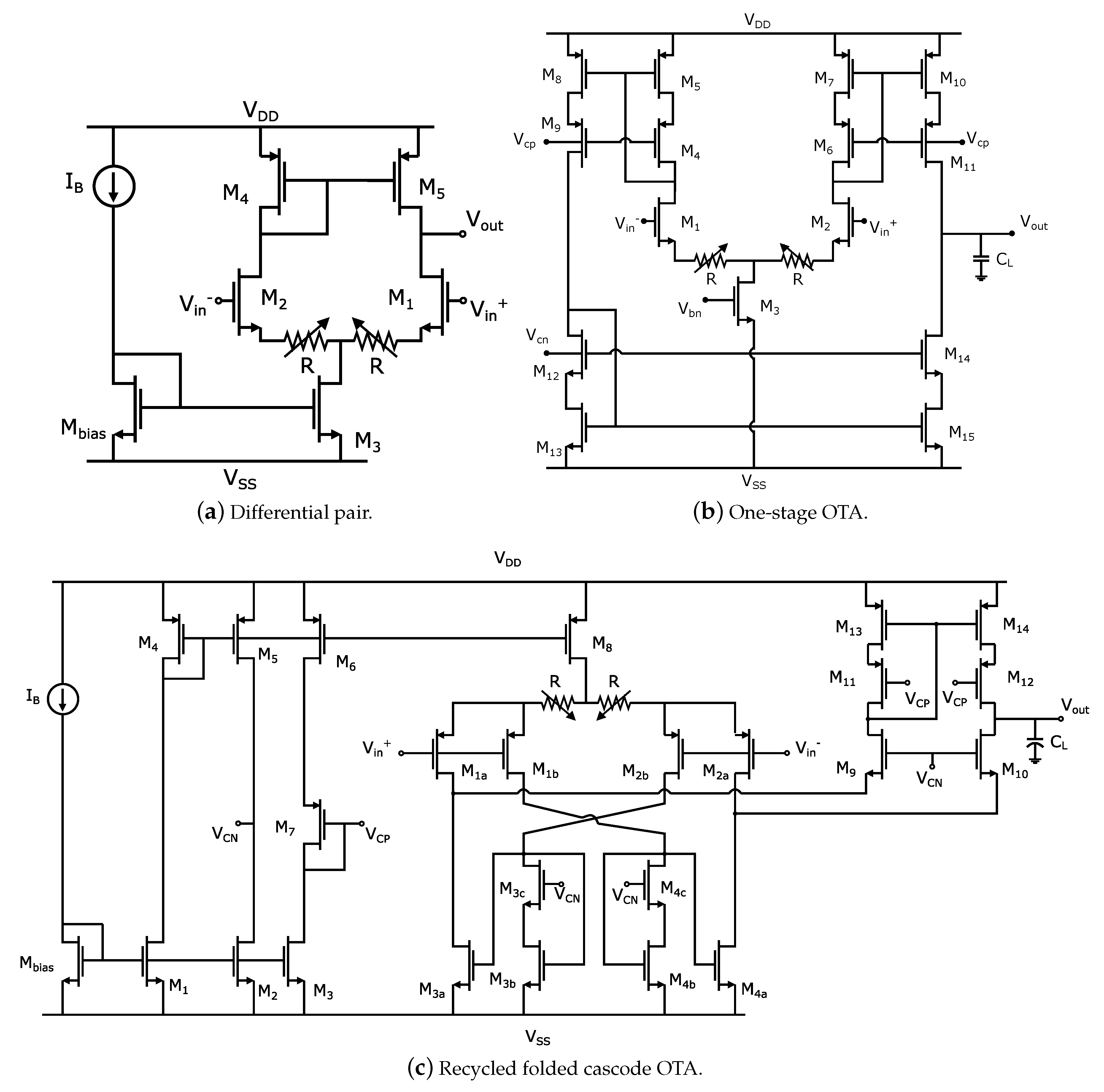
Among the currently available OTA topologies, this work is focused on sizing the CMOS ones shown in Figure 1. The topology given in Figure 1a shows a simple differential amplifier. Figure 1b shows a single-stage OTA and Figure 1c shows the recycled folded-cascode (RFC) OTA proposed in [28], which is a modification from [29], to double the slew rate (SR). 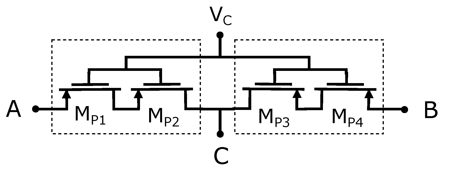All the OTAs have a differential input stage with source degeneration, which allows us to adjust the transconductance ($g_m$) and improve linearity [30], which is required to design an FOCO by using biquadratic OTA-filters. The variable resistors shown in Figure 1 were designed using two P-MOS transistors connected by their gates, as shown in Figure 2.

CMOS OTAs are characterized using an FoM, while other performances and constraints are included according to the application of mono-, multi- and many-objective metaheuristics. The FoM that is considered in this work is given in (1), where the subindex s means small signal. For the many-objective optimization FoM${}_s$, DCGain and CMRR were maximized and power consumption and total silicon area were minimized. During the sizing optimization process, the design variables were the channel width (W) and length (L) of all transistors and the value of the bias current ($I_b$), which were updated within a SPICE netlist-file. These design variables and the control voltage ($V_c$) were encoded into a vector $x\in {\mathbb{R}}^n$, where n represents the problem’s dimension. The vector was defined by $x=[a_1,a_2,...,a_n]$ and each design variable was bounded to the values $a_i\in [2\mathsf{\mu }\mathrm{m},1000\mathsf{\mu }\mathrm{m}]$ for $W_i$, $a_i\in [2\mathsf{\mu }\mathrm{m},10\mathsf{\mu }\mathrm{m}]$ for $L_i$, $a_i\in [10\mathsf{\mu }\mathrm{A},100\mathsf{\mu }\mathrm{A}]$ for $I_{b_i}$ and $a_i\in [-0.9\mathrm{v},0.9\mathrm{v}]$ for $V_{c_i}$. Finally, each constraint was handled as $g\left(x\right)\ge 0$.

$$Fo{M}_s={\displaystyle \frac{GBW\times C_L}{I_b}}$$

(1)

The sizing optimization problem for the OTAs can then be defined as follows:

Search: Widths ($W_i$) and lengths ($L_i$) of each MOS transistor and bias current ($I_{b_i}$) of a CMOS OTA in order to:

Maximize: FoM${}_s$(x), DCGain(x), CMRR(x), -Powerconsumption(x), -TotalMOSarea(x).

Subject to: DC gain $\ge 60$ dB, PM $\ge {45}^{\circ }$, CMRR $\ge 60$ dB, PSRR $\ge 60$ dB, SR $\ge 1$ V/$\mathsf{\mu }$s, $V_{DS}\ge 3(V_{GS}-V_{TH})$ for each MOS transistor and power consumption ≤ 5 mW.

Other inherent constraints that depend on the circuit’s topology were considered, such as, in a differential pair, the W/L sizes of both transistors were equal, as well as some MOS transistors had to be equal when they were part of a current mirror with unity gain.

3. Mono-Objective Algorithms

Mono-objective optimization metaheuristics have the goal of finding the best minimum or maximum value, which corresponds to the solution of a single objective function. The sizing of an analog IC by a mono-objective algorithm provides information on the nature of the optimization problem, but, generally, the algorithm does not provide a set of workarounds that interchange different objectives with each other. However, it is well known that a single-objective metaheuristic provides a final solution or a set of solutions that are really good [31]. In this paper, we applied mono-objective metaheuristics, such as PSO, MOL and DE, to size the OTAs given in Figure 1.

3.1. PSO Algorithm

PSO is a metaheuristic that performs an iterative optimization based on the social behavior of birds or fishes and it is based on the mathematical models given in (2) and (3) [32]. PSO’s behavior is based on a random initialization of a set of particles whose search space was defined and bounded in this work. This process is intended to give favorable initial position and velocity to the particles. The random initialization and the mathematical models given in (2) and (3) allow to change the particles’ position at every iteration and depending on the value of some random parameters, the velocity is adjusted. In this manner, both the position $p_i$ and velocity $v_i$ are updated until a stop criterion is met. In the updating equations $pbest$ and $gbest$ provide information on the particle’s best position and best global position that is measured among all particles. The parameter rand() returns a random and uniform real value between 0 and 1. The constant parameter $c_1$ denotes the confidence of a particle and $c_2$ denotes its confidence in the swarm. In this paper, we set the constant parameter $c_1$ and $c_2$ equal to 2, as recommended in [33].

$$v_i=v_i+c_1\mathrm{rand}\left(\right)(p_{best}-p_i)+c_2\mathrm{rand}\left(\right)(g_{best}-p_i)$$

(2)

$$p_i=p_i+v_i$$

(3)

3.2. MOL Algorithm

Basically, the MOL algorithm is a simplified version of PSO. It is derived from the original behavior of PSO, but, in this case, MOL neglects the best position of a particle [34]. This is conducted by eliminating $pbest$ in (2), which updates to (4), meaning that there is more communication among the particles [35]. Therefore, the MOL algorithm tends to have a purely social behavior, since each particle follows the best among all without looking for another solution on its own. In addition, having a simplified model makes it easier to select the parameters in MOL, which is not easy in PSO. One of these parameters is the inertia weight (w), which is related to facilitating the particles to find better solutions by exploring different directions throughout the values in the search space. In this paper, the parameters in MOL were set to $w=0.95$ and $c_2=2$.

$$v_i=w{v}_i+c_2\mathrm{rand}\left(\right)(g_{best}-p_i)$$

(4)

3.3. DE Algorithm

DE belongs to the class of evolutionary algorithms (EA) that are based on the concepts of the theory of evolution of species proposed by Darwin. DE has two main steps [36], initialization and evolution. In the initialization phase, the population is randomly generated within a determined search space. In the evolution phase, the current population is handled by performing genetic operations, such as mutation, crossover and selection processes, that are executed in the optimization loop until a determined number of generations or a stop criterium is met. Some of the most important advantages of DE are: its simplicity of programming, versus other EAs; its much better performance, considering correctness, speed of convergence and robustness; and the fact that the script can be coded in relatively few lines and that the complexity of the search space is low, considering similar EAs [37].

After the initialization of the population, each individual is mutated and then a new solution $v_{ij}$ is generated from three randomly selected parents, as given in (5). Thereafter, the crossover operation is executed to create a new solution considered as a trial solution, as described in (6). This crossover operation is executed taking a target $x_{ij}$ and a mutant vector $v_{ij}$, with a probability value $P_c$ between 0 and 1. The weighting factors $P_m$ and $P_c$ are the mutant and crossover probability, respectively. Finally, a replacement is carried out by elitist selection, in which the target and trial vectors are compared considering the fitness values. The individual with better fitness is taken and it survives to perform the same optimization process that follows in the next generation, as described in (7). In DE the mutation, crossover and selection process are executed at each generation until a stop criterion is met.

$$v_j=x_{r3j}+P_m(x_{r1j}-x_{r2j})$$

(5)

$$u_j=\left\{\begin{array}{ccccc}{v}_j& \mathrm{if}& rand\left(\right)<P_c& or& j=j_{rand}\\ x_j& & \mathrm{otherwise}\end{array}\right.$$

(6)

$$x_i=\left\{\begin{array}{ccc}{u}_i& \mathrm{if}& f\left(u_i\right)<f\left(x_i\right)\\ x_i& & \mathrm{otherwise}\end{array}\right.$$

(7)

4. Multi-Objective Algorithms

In a given optimization problem, if one can observe that the targets are in conflict with each other, then the solution can be obtained by applying multi-objective metaheuristics. That is, if one objective improves, the other deteriorates and vice versa. The most representative multi-objective metaheuristics are NSGA-II and MOEA/D.

4.1. NSGA-II Algorithm

NSGA-II was proposed by Kalyanmoy Deb in 2002 [38], as a version that improved the original NSGA proposed by Goldberg [39], in which an initial population is partitioned into fronts according to a non-dominance criterion. NSGA-II performs an iterative optimization process, starting from an initial population or a set of individuals; after an evaluation, the individuals with better fitness are selected as parents and evolve according to the concept of natural selection applying genetic operators, such as crossover, mutation and selection, to generate new offsprings. This process is called generation and is repeated until a stop criterion is met.

Its main characteristics are fast non-dominated sorting, computational complexity in the order of $O\left(M{N}^2\right)$, fast ranking function, crowding distance assignment and elitism. It determines a rank value that considers the number of individuals that dominates each solution. NSGA-II performs crowding distance to keep the solution’s diversity in the Pareto front to ensure that each feasible solution is kept at a good crowding distance. The elitism is an operator that executes the fast non-dominated sort approach and crowding distance and selects the individual with the highest ranking.

4.2. MOEA/D Algorithm

MOEA/D is an EA introduced in 2006 [40]. It transforms a multi-objective optimization problem into a set of single optimization problems. Each subproblem is associated to an individual solution and all of them are simultaneously optimized and quantified using utility functions, weight vectors and a reference point. In general, each subproblem is evaluated using only the information of its neighbors as a mechanism of elitism. This characteristic allows us to reduce the computational complexity without affecting the performance and even outperforms NSGA-II.

5. Many-Objective Algorithms

The optimization of problems with more than three objectives is an open research area and shows a great opportunity to improve its performance. The definition of many-objective optimization was introduced by Purshouse and Fleming [41] after observing that multi-objective algorithms based on Pareto optimality presented serious problems as the number of objectives increased.

5.1. NSGA-III Algorithm

NSGA-III is a many-objective metaheuristic proposed in 2013 [42], where, unlike NSGA-II, the solution’s diversity among all individuals in the population is enhanced by supplying and adaptively updating a number of well-spread reference points. According to [43], NSGA-III has a similar framework to NSGA-II, the only difference being the inclusion of representative changes in the selection process. The operations are executed as follows: First, the parent population is randomly initialized; afterwards, the binary tournament selection, crossover and mutation genetic operations take place to generate an offspring population. In the next step, both populations are combined to duplicate the number of individuals that are sorted taking into account their domination level. Half of the best individuals in the combined population are selected to update the population that becomes parent one, ready to execute the same genetic operations in the next generation. The selection process starts with a set of reference points, which are generated by spanning a hyperplane with unit intercepts associated to the objective axis by applying the method for normal boundary intersection, as detailed in [44].

5.2. MOMBI-II Algorithm

MOMBI-II was proposed by Raquel Hernández in [45] and performs a hierarchical ranking of the individuals of a population. MOMBI-II is a metaheuristic capable of handling two or more objectives, since it uses indicators as a selection mechanism to keep the solution’s diversity and also serves, during the optimization process, as a guide for the search or as a stopping criterion. The $R2$ indicator is a very reliable approach that is useful for problems formulated with multi- and many-objective metaheuristics. It is also suitable to compare approximations of different multi-objective optimizers by means of utility functions. One of the main advantages of the $R2$ indicator is the low computational cost and the compatibility with the Pareto front. Therefore, MOMBI-II has the advantage to optimize problems formulated with objectives higher than three and without having problems with Pareto dominance.

6. Sizing OTAs by NSGA-III, MOMBI-II and MOEA/D

The pseudo-codes provided in [46] were modified to maximize FoM${}_s$, differential mode gain and CMRR and minimize the power consumption and the total MOS area. In Algorithms 1–3, the adaptations of the NSGA-III, MOMBI-II and MOEA/D algorithms are shown, respectively. All the algorithms linked SPICE to evaluate the circuit characteristics related to the objective functions, taken from the $\ast .lis$ output file generated by SPICE, and, to reduce execution time, the command. MEASUREMENT was used within the input file $\ast .sp$.

The $\ast .sp$ SPICE input file was encoded by means of subcircuits to perform a direct current (.DC), alternating current (.AC) and transient (.TRAN) analyses. In addition, to avoid modifying this file at each generation, a $\ast .lib$ file was linked with the original netlist. This $\ast .lib$ file had the design variables W, L, $I_b$ and $V_c$. Therefore, the variables obtained from the NSGA-III, MOMBI and MOEAD algorithms were replaced within the $\ast .lib$ file without compromising any analysis in the $\ast .sp$ file.

Algorithm 1 NSGA-III.

procedureNSGA-III($P,Gen,P_c,P_m$)

Create an SPICE netlist of the OTA being optimized

for $i=1:P$ do

Initialize the variables of design W, L, $I_b$ and voltage control ($V_c$), in a random fashion.

Update the design variables values in the SPICE netlist $\ast .lib$

Evaluate the electrical characteristics of the OTA${}_i$ that are saved in the SPICE file ($\ast .lis$)

Normalize objectives and create reference

Compute niche count of reference point

Assign rank based on non-dominated sort

end for

for $it=1:Gen$ do

for $i=1:P$ do

Perform binary tournament selection

Produce offspring using crossover ($P_c$) and mutation ($P_m$) genetic operators

Update the design variables values in the SPICE netlist $\ast .lib$

Evaluate the electrical characteristics of the OTA${}_i$ that are saved in the SPICE file ($\ast .lis$)

Normalize objectives and create reference

Compute niche count of reference point

Perform a fast non-dominated sorting ranking and crowding distance assignment

Select and update the best individuals

end for

end for

end procedure

Algorithm 2 MOMBI-II.

procedure MOMBI($P,Gen,P_c,P_m$)

Create an SPICE netlist of the OTA being optimized

for $i=1:P$ do

Initialize the variables of design W, L, $I_b$ and voltage control ($V_c$), in a random fashion.

Update the design variables values in the SPICE netlist $\ast .lib$

Evaluate the electrical characteristics of the OTA${}_i$ that are saved in the SPICE file ($\ast .lis$)

Calculate $L_1$ and $L_2$ norms

Execute R2 ranking indicator

end for

for $it=1:Gen$ do

for $i=1:P$ do

Perform tournament selection

Produce offspring using crossover ($P_c$) and mutation ($P_m$) genetic operators

Update the design variables values in the SPICE netlist $\ast .lib$

Evaluate the electrical characteristics of the OTA${}_i$ that are saved in the SPICE file ($\ast .lis$)

Execute R2 ranking indicator

Reduce and update the population

end for

end for

end procedure

Algorithm 3 MOEA/D.

procedureMOEA/D($P,Gen,P_c,P_m$)

Create an SPICE netlist of the OTA being optimized

for $i=1:P$ do

Initialize the variables of design W, L, $I_b$ and voltage control ($V_c$), in a random fashion.

Update the design variables values in the SPICE netlist $\ast .lib$

Evaluate the electrical characteristics of the OTA${}_i$ that are saved in the SPICE file ($\ast .lis$)

Calculate the nearest neighbor and the reference point

end for

for $it=1:Gen$ do

for $i=1:P$ do

Produce offspring using crossover ($P_c$) and mutation ($P_m$) genetic operators.

Update the design variables values in the SPICE netlist $\ast .lib$

Evaluate the electrical characteristics of the OTA${}_i$ that are saved in the SPICE file ($\ast .lis$)

Update the reference point

Select the individual with better fitness

end for

end for

end procedure

The optimization process is generally the same for each algorithm; for all of them, it is necessary to specify the number of individuals (P), generations ($Gen$), crossover constant ($P_c$), mutation constant ($P_m$), number of design variables, restrictions and limits for each design variable. However, each algorithm has its own method of sorting, ranking and selecting the best individuals.

7. Optimal Solutions Applying Mono-, Multi- and Many-Objective Metaheuristics

A sized solution provided by a metaheuristic is said to be feasible when it achieves all the target specifications. This section summarizes the sizing of the OTAs applying PSO, MOL and DE as mono-objective; NSGA-II and MOEA/D as multi-objective; and NSGA-III, MOEA/D and MOMBI-II as many-objective metaheuristics. The mono-objective sizing optimization considered the FoM described in Section 2 as the single objective function, with the other electrical characteristics as constraints. The multi-objective sizing considered the optimization of three objectives simultaneously, namely, FoM, DC Gain and power consumption. The many-objective optimization process included five objectives: FoM, DC Gain, power consumption, CMRR and the total MOS area. For each metaheuristic 10 runs were executed, with 100 generations and a population equal to 70 individuals/particles to size the OTAs shown in Figure 1. The target specifications are listed in

Table 1. Target specifications for the sizing of the OTAs shown in Figure 1.

Topology	Differential Pair	One-Stage OTA	RFC OTA
UMC CMOS technology	0.18 $\mathsf{\mu }$m	0.18 $\mathsf{\mu }$m	0.18 $\mathsf{\mu }$m
Voltage supply (V)	±0.9	±0.9	±0.9
C${}_L$ (pF)	≥5	≥5	≥5
DC Gain (dB)	≥60	≥60	≥60
GBW (MHz)	≥10	≥10	≥10
PM (°)	≥50	≥50	≥50
CMRR (dB)	≥60	≥60	≥60
SR+ (V/$\mathsf{\mu }$s)	≥5	≥5	≥5
SR− (V/$\mathsf{\mu }$s)	≥5	≥5	≥5
PSRR+ (dB)	≥60	≥60	≥60
PSRR− (dB)	≥60	≥60	≥60
Power consumption (mW)	≤5	≤5	≤5
Vmax (V)	≥0.5	≥0.5	≥0.5
Vmin (V)	≤−0.5	≤−0.5	≤−0.5

.

Although the optimization process is similar for each metaheuristic, the behavior is quite different. In PSO, the particles search in their vicinity both individually and as a group in order to find better positions according to their updating equations defined in (2) and (3), while, the behavior of MOL, despite being a variation of PSO, is purely social, that is, all the particles search together for the global best position. DE is an evolution-based algorithm, finding better solutions through genetic processes such as mutation, crossover and selection. The main advantage of applying mono-objective optimization such as PSO, MOL and DE is that the cost of the objective function is taken to the limit. This means that they are capable of reaching very good values; however, their great disadvantage is that the other characteristics are under a threshold, defined as constraints, limiting their performance. In multi- and many-objective algorithms, the main goal is devoted to enhancing the trade-off among different objectives. The most popular multi-objective algorithm in recent decades is the NSGA-II, whose main characteristics are the diversity, the convergence and the robustness given to the solutions that can be sketched in the Pareto front. However, its performance is limited by the number of objectives. For this reason, this work highlights the advantages of the many-objective metaheuristics to size CMOS amplifiers, which have a huge number of target specifications. The main characteristics of the many-objective algorithms applied herein are: NSGA-III is a variation of the well-known NSGA-II; MOEA/D is a decomposition algorithm with the advantage of handling more than three objectives at the same time; and MOMBI-II has the advantage of using performance indicators as a selection mechanism.

The best solutions of 10 runs for each metaheuristic are shown in

Table 2. Best solutions (in boldface) obtained by applying mono-, multi- and many-objective algorithms to size the differential pair shown in Figure 1a.

	Mono-Objective				Multi-Objective			Many-Objective
	PSO	MOL	DE		NSGA-II	MOEA/D		NSGA-III	MOEA/D	MOMBI-II
FoM${}_s$	1569	1625	1671		1622	1700		1615	1610	1637
DCGain (dB)	35	30	33		33	32		36	36	35
CMRR (dB)	56	59	56		62	60		64	64	65
Power consumption ($\mathsf{\mu }$W)	625	863	832		782	818		773	787	751
MOS Area ($\mathsf{\mu }$m${}^2$)	1568.3	1550.9	1659.8		1762.6	1797.7		1439	1442.5	1679.2
GBW (MHz)	12.55	17.87	17.72		16.21	17.68		15.82	16.1	15.71
PM (°)	88	89	89		85	89		87	87	88
PSRR+ (dB)	42	41	40		45	41		50	50	47
PSRR− (dB)	62	68	62		67	63		83	81	75
SR+ (V/$\mathsf{\mu }$s)	7	10	10		10	10		10	10	9
SR− (V/$\mathsf{\mu }$s)	6	8	8		7	8		8	8	7
Vmax (V)	0.7	0.7	0.8		0.7	0.7		0.6	0.6	0.6
Vmin (V)	−0.3	−0.5	−0.5		−0.5	−0.5		−0.5	−0.5	−0.5
W1 [M1,M2] ($\mathsf{\mu }$m)	76.68	90	84.96		88.92	89.91		55.08	52.02	89.46
W2 [Mb,M3] ($\mathsf{\mu }$m)	38.88	49.95	56.79		85.5	87.3		62.28	63	72.99
W3 [M4,M5] ($\mathsf{\mu }$m)	32.85	7.29	29.79		23.49	15.48		11.79	12.59	7.83
W4 [Mp1-Mp4] ($\mathsf{\mu }$m)	88.74	90	90		72.45	90		81.91	86.04	85.32
L1 [M1,M2] ($\mathsf{\mu }$m)	0.81	0.9	0.9		1.17	0.81		0.54	0.81	0.99
L2 [Mb,M3] ($\mathsf{\mu }$m)	0.99	0.9	0.81		1.17	1.17		0.9	0.9	1.08
L3 [M4,M5] ($\mathsf{\mu }$m)	0.63	0.18	0.27		1.08	0.27		0.9	0.9	0.54
L4 [Mp1-Mp4] ($\mathsf{\mu }$m)	0.18	0.18	0.18		0.18	0.18		0.18	0.18	0.18
Ib ($\mathsf{\mu }$A)	40	55	53		50	52		49	50	48
Vctrl (V)	−5	−5	−5		−5	−5		−4	−3	−4

,

Table 3. Best solutions (in boldface) obtained by applying mono-, multi- and many-objective algorithms to size the one-stage OTA shown in Figure 1b.

	Mono-Objective				Multi-Objective			Many-Objective
	PSO	MOL	DE		NSGA-II	MOEA/D		NSGA-III	MOEA/D	MOMBI-II
FoM${}_s$	1613	1664	1621		1670	1675		1639	1701	1664
DCGain (dB)	60.75	60.27	68		71.13	66		72	60.78	61.20
CMRR (dB)	89.75	88.27	95		99	95		95	90	81
Power consumption (mW)	3.07	3.03	2.2		2	2.2		1.94	1.97	1.96
MOS Area ($\mathsf{\mu }$m${}^2$)	3183	3681.6	3993.4		3302.6	3400.9		3151.2	3242.5	3233.1
GBW (MHz)	25.17	26.29	19.13		17.04	19.10		16.39	17.35	16.97
PM (°)	81	82	81		80	83		81	83	81
PSRR+ (dB)	77	77	93		89	87		88	76	76
PSRR− (dB)	62	61	70		72	67		73	62	62
SR+ (V/$\mathsf{\mu }$s)	5	6	5		4	4		4	3	4
SR− (V/$\mathsf{\mu }$s)	5	5	3		3	3		3	3	3
Vmax (V)	0.6	0.6	0.5		0.5	0.5		0.5	0.5	0.5
Vmin (V)	−0.5	−0.5	−0.5		−0.5	−0.5		−0.5	−0.5	−0.5
W1 [M1,M2] ($\mathsf{\mu }$m)	180	180	127.17		124.11	142.65		96.75	141.12	101.7
W2 [M3,M12-M16,Mb] ($\mathsf{\mu }$m)	20.97	31.32	35.73		17.01	33.57		26.82	27.27	32.94
W3 [M4-M11,M17] ($\mathsf{\mu }$m)	26.37	24.93	47.7		29.43	18.81		32.94	12.33	17.46
W4 [Mp1-Mp4] ($\mathsf{\mu }$m)	126.45	180	175.59		178.2	179.91		170.73	179.28	178.92
L1 [M1,M2] ($\mathsf{\mu }$ m)	1.71	1.53	1.44		1.62	1.71		1.35	1.8	1.35
L2 [M3,M12-M16,Mb] ($\mathsf{\mu }$m)	1.08	0.72	0.72		0.99	0.54		1.53	0.81	1.62
L3 [M4-M11,M17] ($\mathsf{\mu }$m)	0.18	0.18	0.36		0.27	0.27		0.27	0.18	0.18
L4 [Mp1-Mp4] ($\mathsf{\mu }$m)	0.18	0.18	0.36		0.18	0.18		0.18	0.18	0.18
Ib ($\mathsf{\mu }$A)	78	79	59		51	57		50	51	51
Vc (V)	−3	−5	−5		−5	−5		−5	−5	−5

and

Table 4. Best solutions (in boldface) obtained by applying mono-, multi- and many-objective algorithms to size the RFC OTA shown in Figure 1c.

	Mono-Objective				Multi-Objective			Many-Objective
	PSO	MOL	DE		NSGA-II	MOEA/D		NSGA-III	MOEA/D	MOMBI-II
FoM${}_s$	2544	3987	3987		3431	3838		3475	4190	3564
DCGain (dB)	72	74	69		74	68		73	66	74
CMRR (dB)	98	101	95		110	98		108	94	108
Power consumption (mW)	3.6	3.19	4.11		2.85	4.33		2.84	4.12	2.23
MOS Area ($\mathsf{\mu }$m${}^2$)	4133.1	3788	4231.7		1822.4	4467.8		2601.75	3808.53	3829.37
GBW (MHz)	24.93	27.14	39.87		24.71	41.45		25.02	40.22	20.67
PM (°)	62	62	70		80	70		75	73	71
PSRR+ (dB)	72	74	69		74	67		72	65	75
PSRR− (dB)	113	108	116		110	95		120	87	105
SR+ (V/$\mathsf{\mu }$s)	9	7	11		7	11		7	11	7
SR− (V/$\mathsf{\mu }$s)	26	20	33		22	30		20	20	10
Vmax (V)	0.5	0.5	0.5		0.5	0.5		0.5	0.5	0.5
Vmin (V)	−0.8	−0.8	−0.8		−0.8	−0.8		−0.8	−0.8	−0.8
W1 [M1-M3,Mb] ($\mathsf{\mu }$m)	50.94	6.21	54.09		17.64	74.7		38.52	36.72	58.05
W2 [M4-M8] ($\mathsf{\mu }$m)	56.7	25.56	70.65		28.62	90		29.88	89.01	59.76
W3 [M1a,M1b.M2a,M2b] ($\mathsf{\mu }$m)	90	90	89.19		47.16	90		47.34	69.66	82.71
W4 [M3a,M3b.M4a,M4b] ($\mathsf{\mu }$m)	12.69	12.24	15.84		1.62	17.46		7.2	16.83	3.69
W5 [M3c,M4c] ($\mathsf{\mu }$m)	18.9	0.9	0.9		1.44	0.9		5.76	0.9	8.73
W6 [M9,M10] ($\mathsf{\mu }$m)	34.83	39.96	38.43		14.13	42.84		14.04	45.99	33.03
W7 [M11,M12] ($\mathsf{\mu }$m)	77.76	90	68.4		27.18	42.03		34.11	37.62	46.35
W8 [M13,M14] ($\mathsf{\mu }$m)	90	90	51.66		20.7	38.52		20.52	28.71	39.24
W9 [M13,M14] ($\mathsf{\mu }$m)	43.47	90	90		45	90		89.1	89.73	81.27
L1 [M1-M3,Mb] ($\mathsf{\mu }$m)	0.9	0.18	0.45		0.36	0.54		0.45	0.36	0.81
L2 [M4-M8] ($\mathsf{\mu }$m)	0.27	0.18	0.36		0.27	0.36		0.27	0.36	0.45
L3 [M1a,M1b.M2a,M2b] ($\mathsf{\mu }$m)	0.63	0.9	0.54		0.45	0.54		0.45	0.45	0.81
L4 [M3a,M3b.M4a,M4b] ($\mathsf{\mu }$m)	0.72	0.9	0.45		0.63	0.45		0.72	0.45	0.63
L5 [M3c,M4c] ($\mathsf{\mu }$m)	0.9	0.9	0.9		0.54	0.72		0.54	0.9	0.72
L6 [M9,M10] ($\mathsf{\mu }$m)	0.9	0.9	0.54		0.72	0.54		0.81	0.54	0.81
L7 [M11,M12] ($\mathsf{\mu }$m)	0.36	0.9	0.9		0.54	0.72		0.45	0.54	0.54
L8 [M13,M14] ($\mathsf{\mu }$m)	0.72	0.45	0.27		0.27	0.27		0.27	0.18	0.45
L9 [M13,M14] ($\mathsf{\mu }$m)	0.9	0.18	0.18		0.36	0.18		0.36	0.18	0.18
Ib ($\mathsf{\mu }$A)	49	34	50		36	54		36	48	29
Vctrl (V)	−5	−5	−5		−5	−3		−5	−5	−3

, for sizing the differential pair, one-stage and RFC OTA, respectively. The five objectives functions FoM, DC gain, CMRR, power consumption and total MOS area values are listed in the first five lines. The first three characteristics are maximized while the other two are minimized. The other performances, such as GBW, phase margin, PSRR±, SR± and the maximum and minimum output voltage, were handled as constraints. Below Vmin, we list the best sizes of the MOS transistors for each metaheuristic, the bias current and voltage control. In each Table, the best solution values are given in bold face.

As it can be seen, after analyzing these solutions, the metaheuristics with the best performance were, in general, the many-objective ones, since at least one improved the performance of the mono- and multi-objective metaheuristics. They also improved the trade-offs among the five objectives. It can also be pointed out that the mono-objective metaheuristics had a better performance than the multi-objective ones and even their solutions were quite close to the solutions found by the many-objective metaheuristics.

The execution times of the three types of optimization algorithms, known as mono-, multi- and many-objective, are given in

Table 5. Execution time for the optimization of the CMOS differential pair applying mono-, multi- and many-objective metaheuristics.

RUN		PSO	MOL	DE	NSGA-II	MOEA/D	NSGA-III	MOEA/D	MOMBI-II
1		3993.06	4072.61	4132.43	3999.83	4024.54	3849.46	4076.67	4103.54
2		4012.32	4126.72	4345.43	4014.54	4084.33	3934.54	4054.65	4204.6
3		4023.34	4092.3	4276.65	4037.83	4025.25	4054.34	4076.87	4112.43
4		4087.75	4152.54	4185.54	4048.54	4075.63	3945.67	4023.43	4165.73
5	TIME (s)	3996.54	4083.43	4099.54	4083.83	4083.37	3975.54	4103.43	4183.54
6		4011.23	4078.54	4113.43	4085.63	4130.68	3945.76	4098.76	4192.04
7		4085.65	4118.20	4056.65	4053.89	4120.20	4001.2	4034.54	4095.94
8		4123.43	4112.32	4184.54	4011.37	4234.04	3854.65	4076.54	4099.01
9		3999.43	4091.37	4234.54	4140.91	4092.39	4012.04	4011.02	4111.49
10		4023.87	4080.32	4096.23	4026.41	4040.55	4011.23	4023.46	4125.85

,

Table 6. Execution time for the optimization of the CMOS One-stage OTA applying mono-, multi- and many-objective metaheuristics.

RUN		PSO	MOL	DE	NSGA-II	MOEA/D	NSGA-III	MOEA/D	MOMBI-II
1		4465.97	4619.33	4865.65	4356.78	4463.37	4482.75	4462.87	4515.42
2		4487.65	4608.82	4794.56	4457.83	4469.42	4479.13	4470.85	4535.48
3		4356.76	4650.51	4732.45	4430.5	4502.08	4481.45	4476.88	4489.93
4		4443.33	4614.17	4765.76	4395.67	4423.88	4496.56	4509.89	4485.52
5	TIME (s)	4565.65	4621.69	4723.54	4321.83	4422.46	4503.54	4469.99	4478.65
6		4506.54	4615.45	4798.76	4440.02	4503.48	4476.75	4495.9	4500.06
7		4546.04	4619.58	4876.04	4523.82	4437.80	4341.21	4501.62	4475.89
8		4596.49	4621.72	4865.76	4407.52	4473.64	4337.42	4483.24	4445.69
9		4610.43	4654.85	4852.32	4402.02	4510.33	4339.46	4469.87	4440.81
10		4587.49	4647.79	4796.76	4327.84	4426.63	4345.94	4494.58	4458.78

and

Table 7. Execution time for the optimization of the CMOS RFC OTA applying mono-, multi- and many-objective metaheuristics.

RUN		PSO	MOL	DE	NSGA-II	MOEA/D	NSGA-III	MOEA/D	MOMBI-II
1		6055.67	6178.39	6257.65	4385.11	4383.46	4432.76	4326.04	4348.96
2		5179.69	5094.2	6198.54	4384.37	4395.71	4356.76	4356.93	4335.78
3		5167.54	5151.41	6247.04	4363.75	4379.29	4387.59	4331.31	4322.6
4		5134.35	5134.54	6199.54	4430.54	4401.43	4486.8	4361.43	4389.57
5	TIME (s)	5219.43	5101.06	6232.43	4404.72	4411.41	4369.42	4329.26	4343.17
6		5037.33	4963.97	6190.02	4369.20	4330.41	4346.49	4330.38	4272.7
7		7093.37	4930.22	6274.54	4399.44	4303.9	4340.29	4362.76	4253.35
8		7207.78	4909.35	6345.79	4345.93	4401.47	4393.82	4305.92	4230.98
9		5132.1	4959.62	6324.65	4492.46	4376.38	4347.56	4325.97	4241.51
10		5099.69	4955.7	6290.08	4412.42	4401.47	4346.15	4324.21	4346.89

for the differential pair, one-stage OTA and RFC-OTA, respectively.

8. OTA-Based Fractional-Order Chaotic Oscillator

The usefulness of sizing OTAs by many-objective metaheuristics is demonstrated herein by selecting an optimized OTA to design a fractional-order integrator, whose design robustness is verified by performing process, voltage and temperature (PVT) variations and Monte Carlo analysis. The robust OTA-based fractional-order integrator was employed in the design of a fractional-order chaotic oscillator (FOCO) taken from [47] and given in (8). This FOCO had chaotic oscillation when $a=2.05$, $b=1.12$ and $c=0.42$, with initial conditions $x_0=0.1$ and $y_0=z_0=0$. 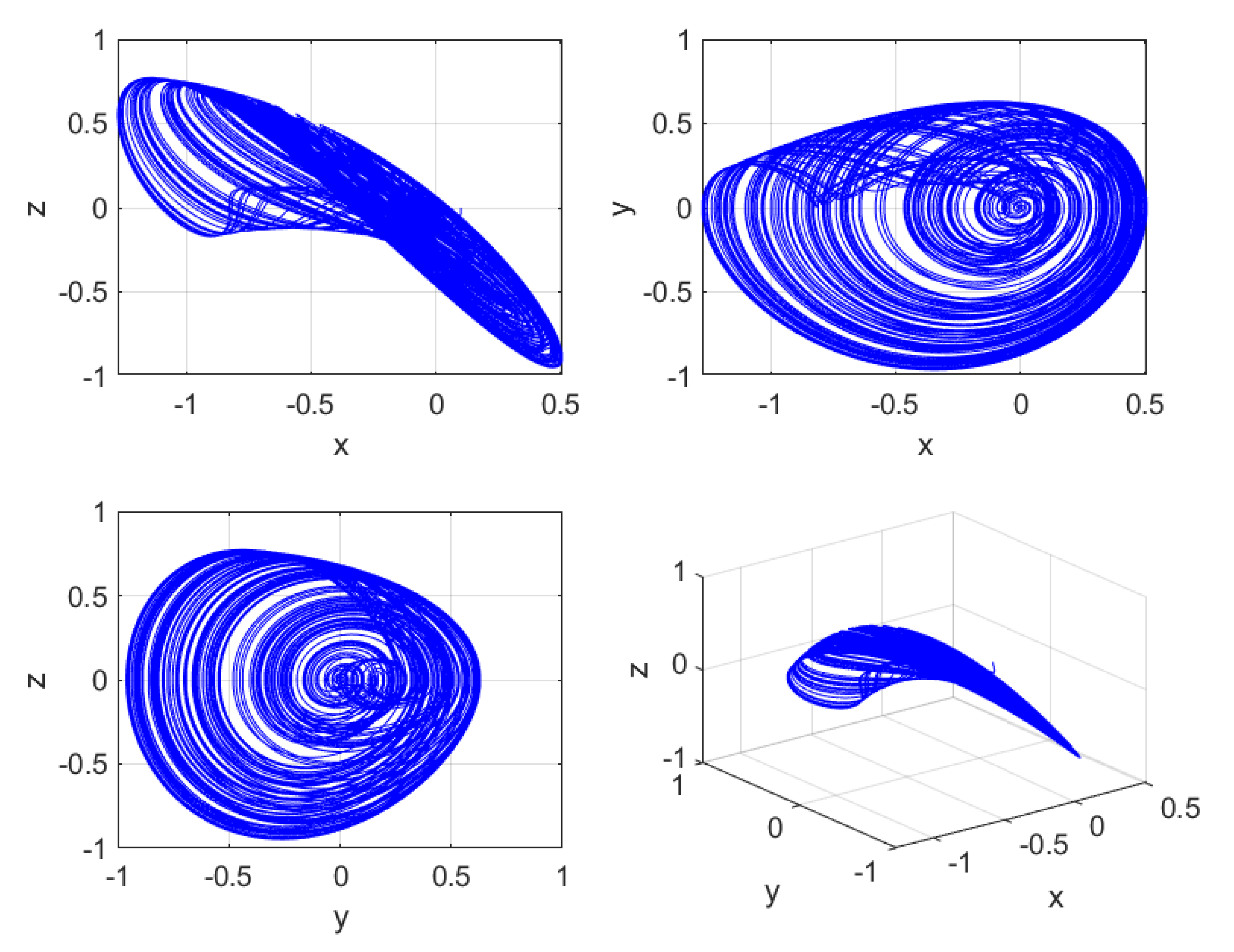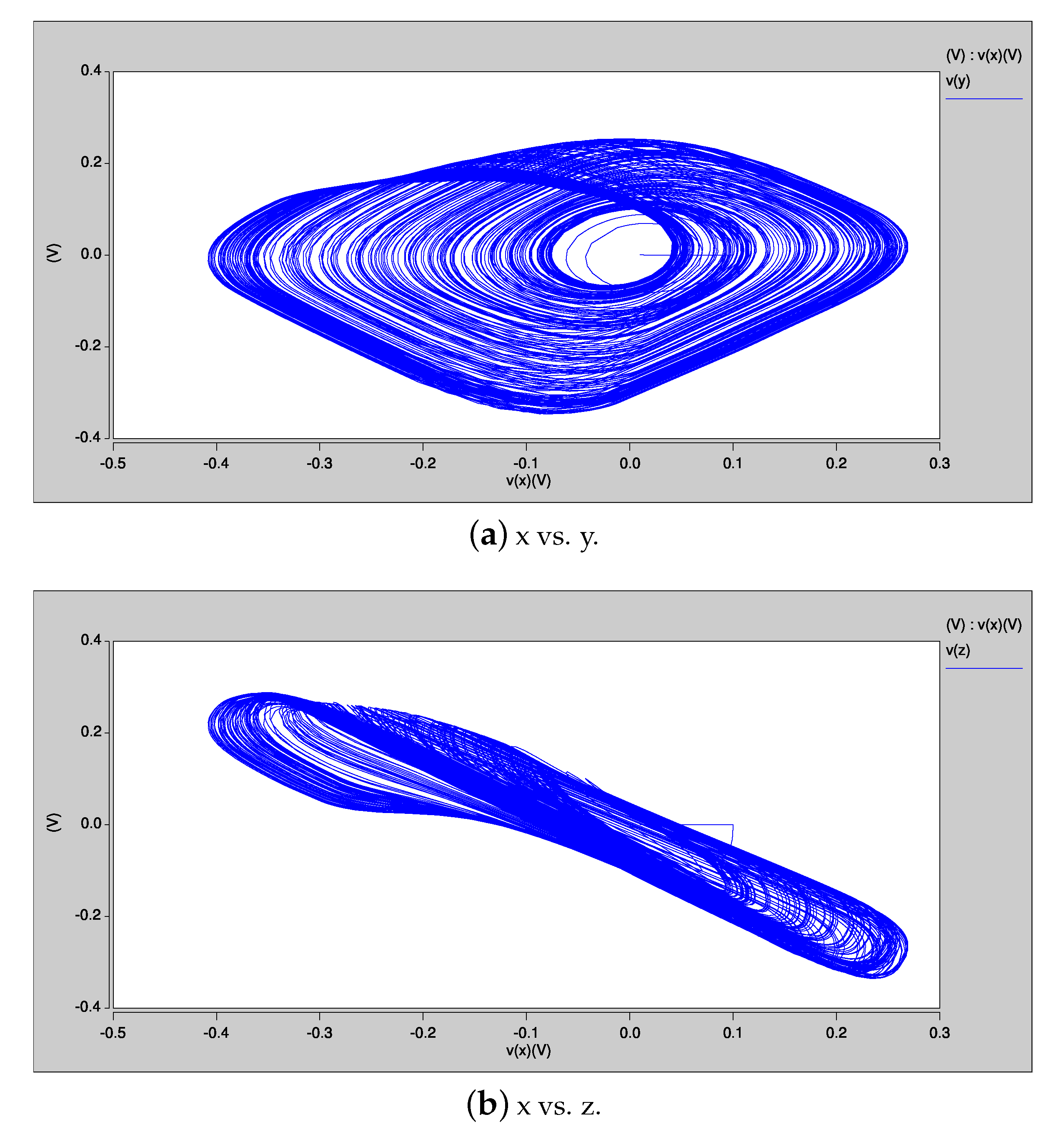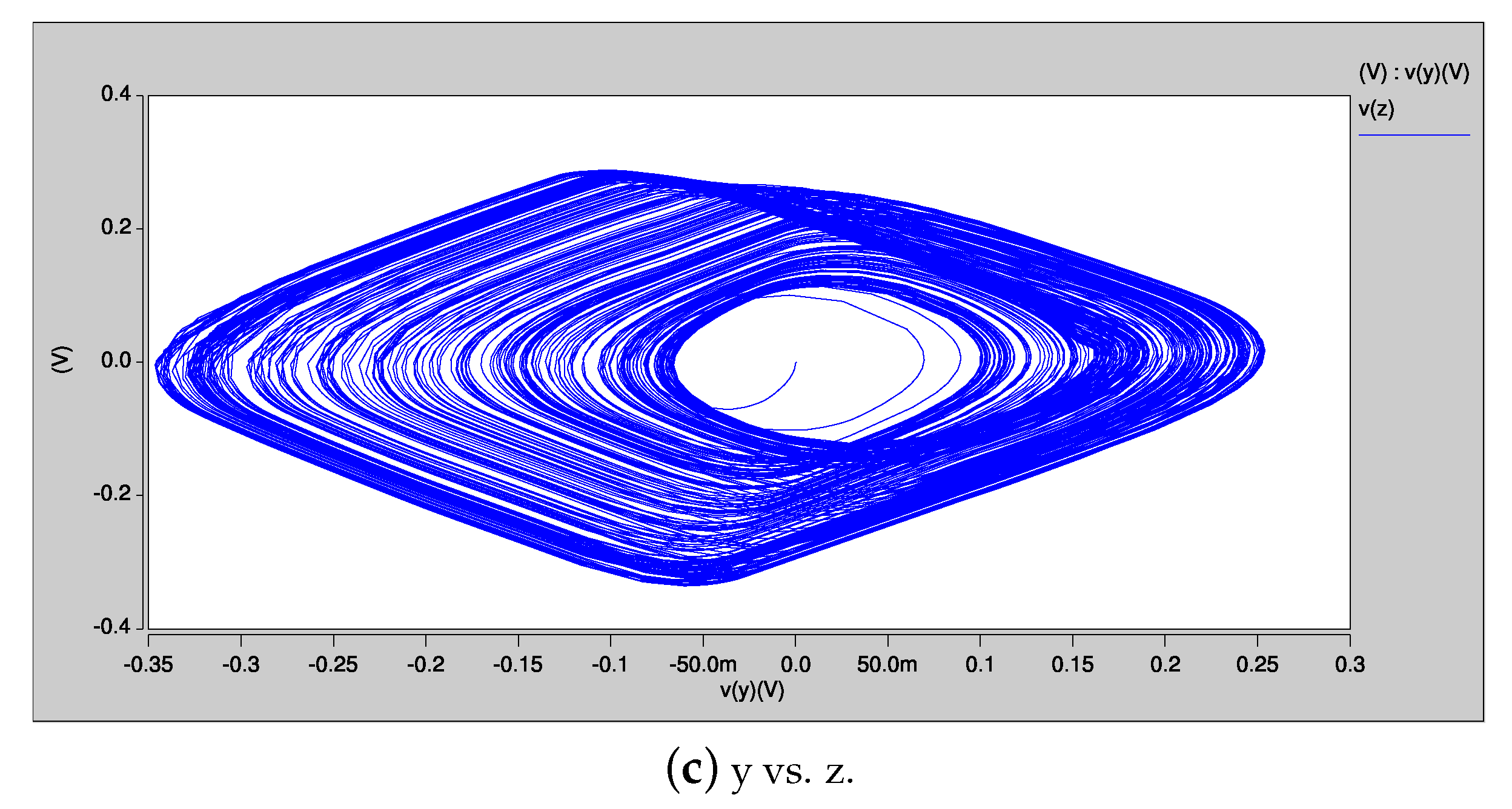Figure 3 shows the portraits of (8), in which the state variables are plotted against each other to generate the attractors. It can be appreciated that the amplitudes of the state variables are below 1, so that it is suitable for CMOS design using a UMC technology at 180 nm.

$$\begin{array}{c}{s}^{0.9}X\left(s\right)=Y\left(s\right)\hfill \\ s^{0.9}Y\left(s\right)=Z\left(s\right)\hfill \\ s^{0.9}Z\left(s\right)=-aX\left(s\right)-bY\left(s\right)-cZ\left(s\right)-3X\left(s\right)\ast X\left(s\right)\hfill \end{array}$$

(8)

Considering the system of equations from (8), one can see that the electronic implementation can be performed using amplifiers, adders/subtractors and one multiplier to evaluate $X\left(s\right)\ast X\left(s\right)$. In addition, a fractional-order integrator is also necessary, which, according to [48], can be approximated by $H\left(s\right)=1/s^{0.9}$, which is modeled by (9).

$$H\left(s\right)={\displaystyle \frac{1}{s^{0.9}}}\approx {\displaystyle \frac{2.2675(s+1.292)(s+215.4)}{(s+0.01292)(s+2.154)(s+359.4)}}$$

(9)

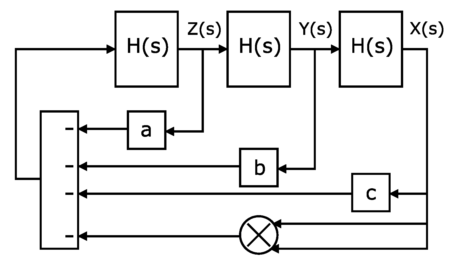
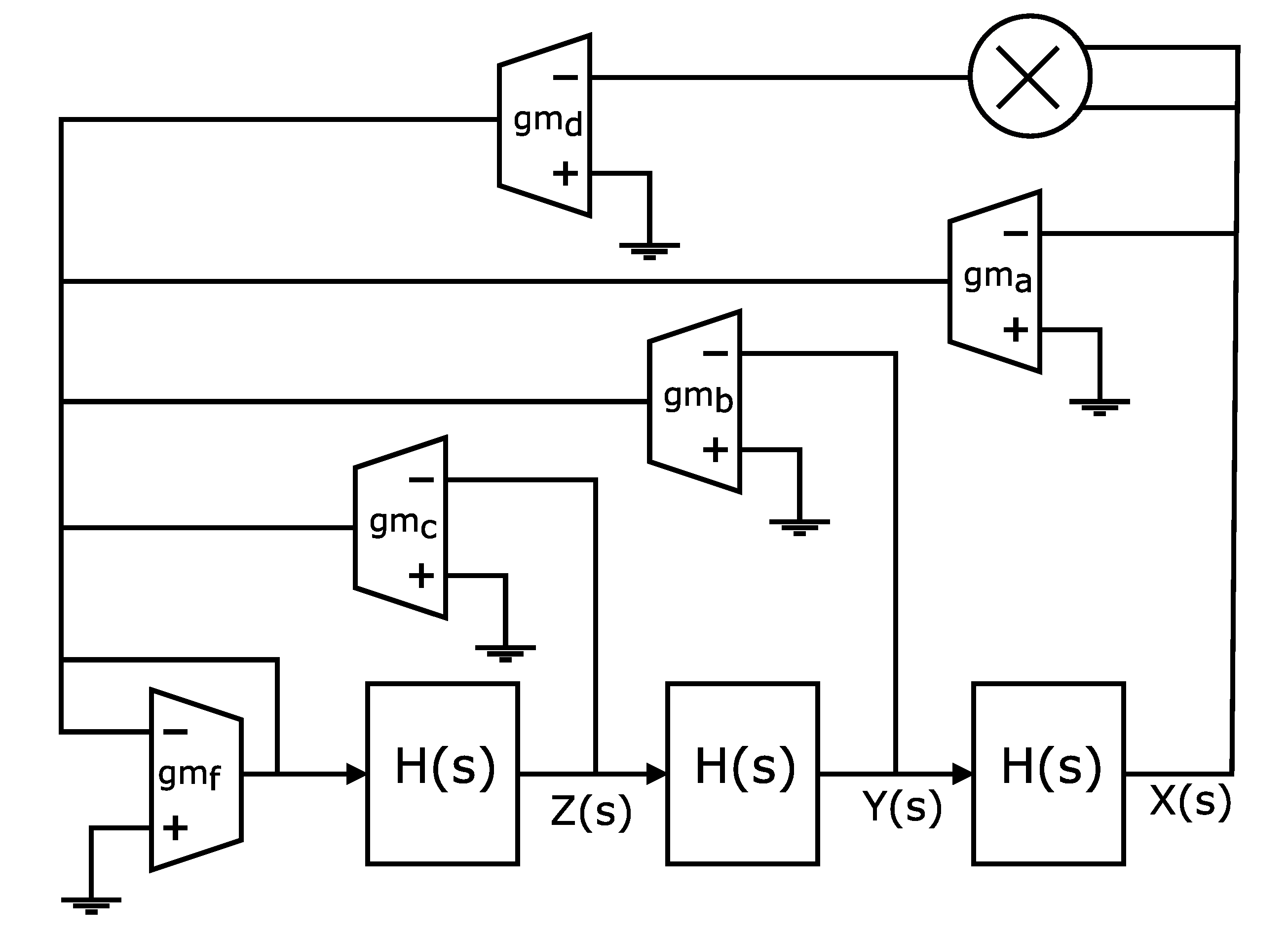
8.1. Building Blocks

Figure 4 shows the block diagram description to implement (8), where the blocks labeled as $H\left(s\right)$ describe the fractional-order integrator $H\left(s\right)$ = ${\displaystyle \frac{1}{s^{0.9}}}$, given in (9). The blocks labeled a, b and c represent the constants of the system in (8). These blocks could be replaced with OTAs, which converted an input voltage into an output current; these currents, in turn, were added to the currents of the other blocks and converted back to voltage at the adder block output. Most of the blocks needed to design the FOCO could be implemented using an OTA with adjustable $g_m$ [49]. In this section, we use the one-stage OTA depicted in Figure 1b. 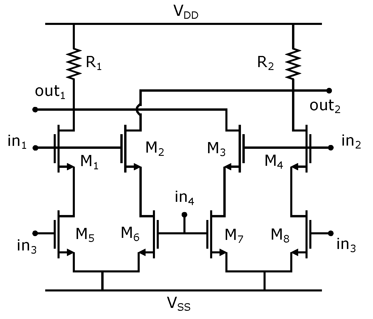The convolution $X\left(s\right)\ast X\left(s\right)$ observed in the state variable $Z\left(s\right)$ could be evaluated by the CMOS four-quadrant multiplier designed in [49] and is shown in Figure 5.

8.2. Fractional-Order Integrator Design Using an OTA-C Biquadratic Filter and an OTA-C Low-Pass Filter

To carry out the design of the fractional-order integrator, the transfer function in (9) was decomposed into two functions, to have $H\left(s\right)$ = $H_1\left(s\right)H_2\left(s\right)$, one of second-order and one of first-order, as given in (10) and (11), respectively. These functions were designed using an OTA-C biquadratic and first-order active filters, as shown in Figure 6, whose topologies were taken from [21]. The circuit transfer functions are given in (12) for the biquadratic and in (13) for the low-pass filters.

$$H_1\left(s\right)={\displaystyle \frac{s^2+216.6920s+278.2968}{s^2+361.5540s+774.1476}}$$

(10)

$$H_2\left(s\right)={\displaystyle \frac{2.2675}{s+0.01292}}$$

(11)

$$Vo={\displaystyle \frac{{\displaystyle \frac{g{m}_{1}g{m}_2}{C_1{C}_2}}{V}_1+s{\displaystyle \frac{g{m}_2}{C_2}}{V}_2+{\displaystyle \frac{g{b}_{0}g{m}_2}{C_1{C}_2}}{V}_3+s^2{V}_4+s{\displaystyle \frac{g{b}_1}{C_2}}{V}_5}{s^2+{\displaystyle \frac{g{m}_2}{C_2}}s+{\displaystyle \frac{g{m}_{1}g{m}_2}{C_1{C}_2}}}}$$

(12)

$$Vo={\displaystyle \frac{g{m}_1/C}{s+g{m}_2/C}}Vi$$

(13)

From $H_1\left(s\right)$ and (12) and by setting $V_1=V_2=0$ and $V_3=V_4=V_5=V_i$, the transfer function of the OTA-based circuit shown in Figure 6a was rewritten as given in (14).

$$H_1\left(s\right)={\displaystyle \frac{s^2+{\displaystyle \frac{g{b}_1}{C_2}}s+{\displaystyle \frac{g{b}_{0}g{m}_2}{C_1{C}_2}}}{s^2+{\displaystyle \frac{g{m}_2}{C_2}}s+{\displaystyle \frac{g{m}_{1}g{m}_2}{C_1{C}_2}}}}={\displaystyle \frac{s^2+216.6920s+278.2968}{s^2+361.5540s+774.1476}}$$

(14)

The design of the biquadratic filter was performed as follows: If $g{b}_0=500\mathsf{\mu }$A/V, the capacitor values are obtained as $C_2=g{b}_1/216.6920=2.3\mathsf{\mu }$F and $C_1=g{b}_{0}g{m}_2/$$278.2968C_2=650\mathsf{\mu }$F. In this manner, $g{m}_2=361.5540C_2=830\mathsf{\mu }$A/V and $g{m}_1=774.1476C_1{C}_2/g{m}_2=1.4$ m A/V. For the low-pass filter shown in Figure 6b, if $g{m}_1=500\mathsf{\mu }$A/V, the capacitor value is $C_1=g{m}_1/2.2675=220\mathsf{\mu }$F; therefore, $R_1=1/0.01292C=350$ K$\mathrm{\Omega }$. 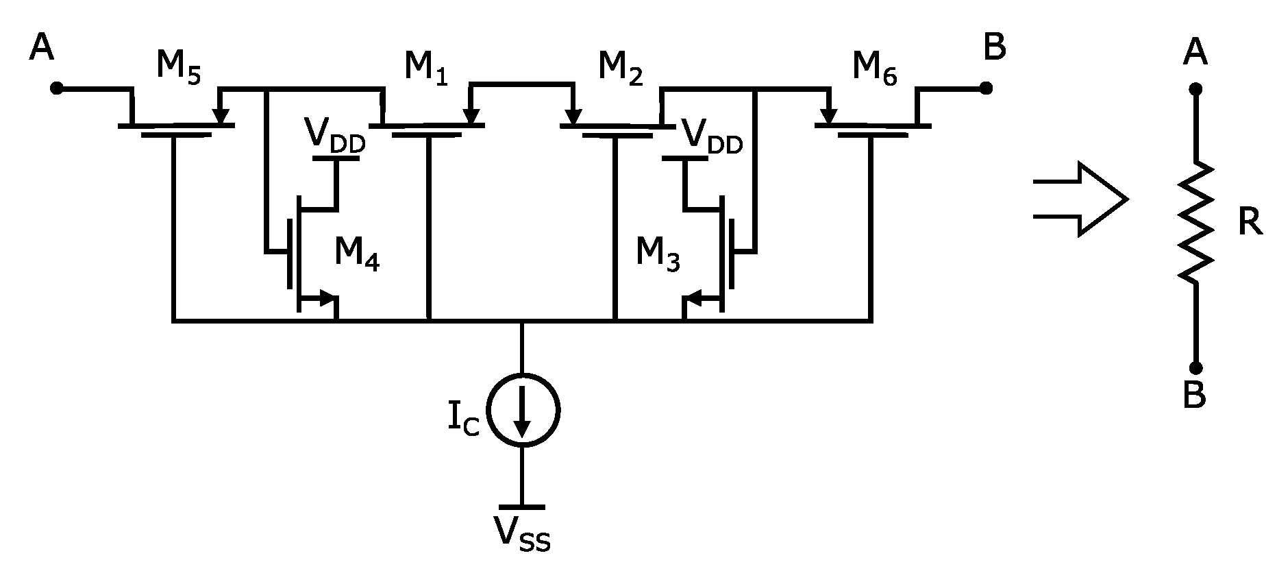In order to achieve a high resistance value, the resistor shown in Figure 7 was implemented [50]. The main advantage of this resistor relies on reaching high resistance values with a good linearity range. In practice, the value of R in Figure 8 was adjusted to 400 K$\mathrm{\Omega }$ to adjust the frequency response of the fractional-order integrator.

We propose the OTA-based design of the fractional-order integrator shown in Figure 9. It includes a biquadratic OTA-C filter in cascade connection with the low-pass OTA filter. As mentioned in [49], it was necessary to consider that the input port had to include the filter embedding the largest zero and the largest pole.

The frequency response of the fractional-order integrator is sketched in Figure 9, which shows the comparison between the ideal response simulated in MatLab of the transfer function given in (9) and its CMOS design using 180 nm UMC technology using the three OTA topologies shown in Figure 1. The sizes of the OTA were taken for the one-stage OTA applying MOEA/D for five objectives. To measure the symmetry of the output signal of the OTA, we used the methodology proposed in [51], in which the output signal must have an absolute minimum value higher than 90% of the absolute maximum signal. In Figure 9, the good agreement between the MatLab and the CMOS implementations of the fractional-order integrator can be appreciated.

8.3. PVT and Monte Carlo Analysis of the Fractional-Order Integrator

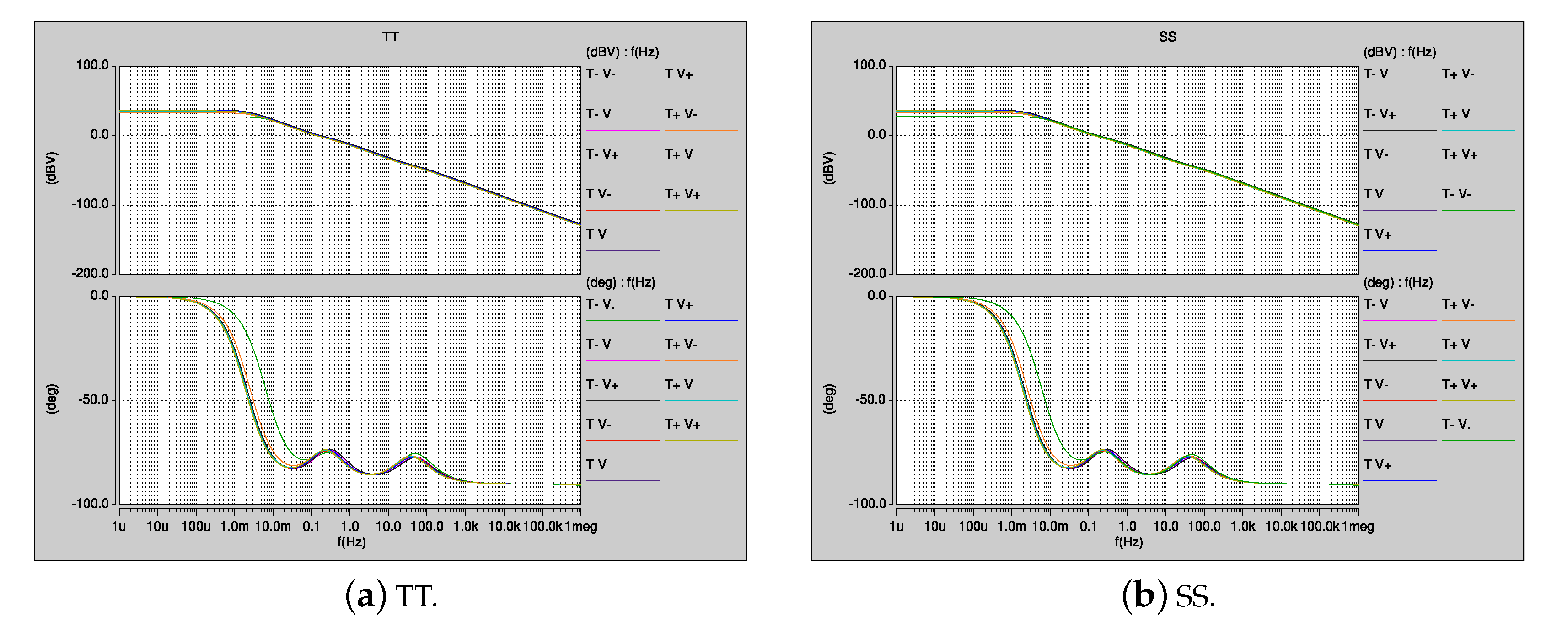
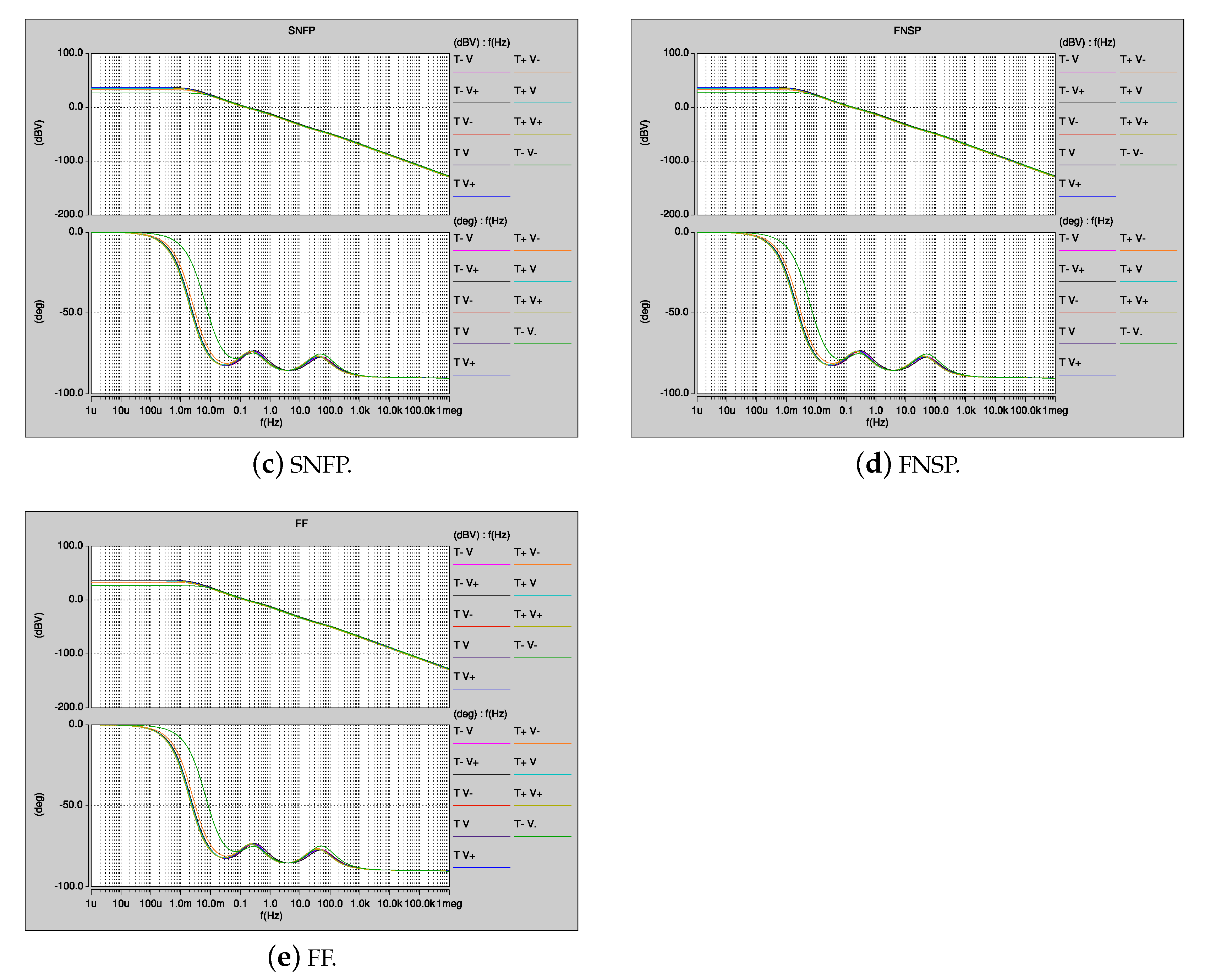
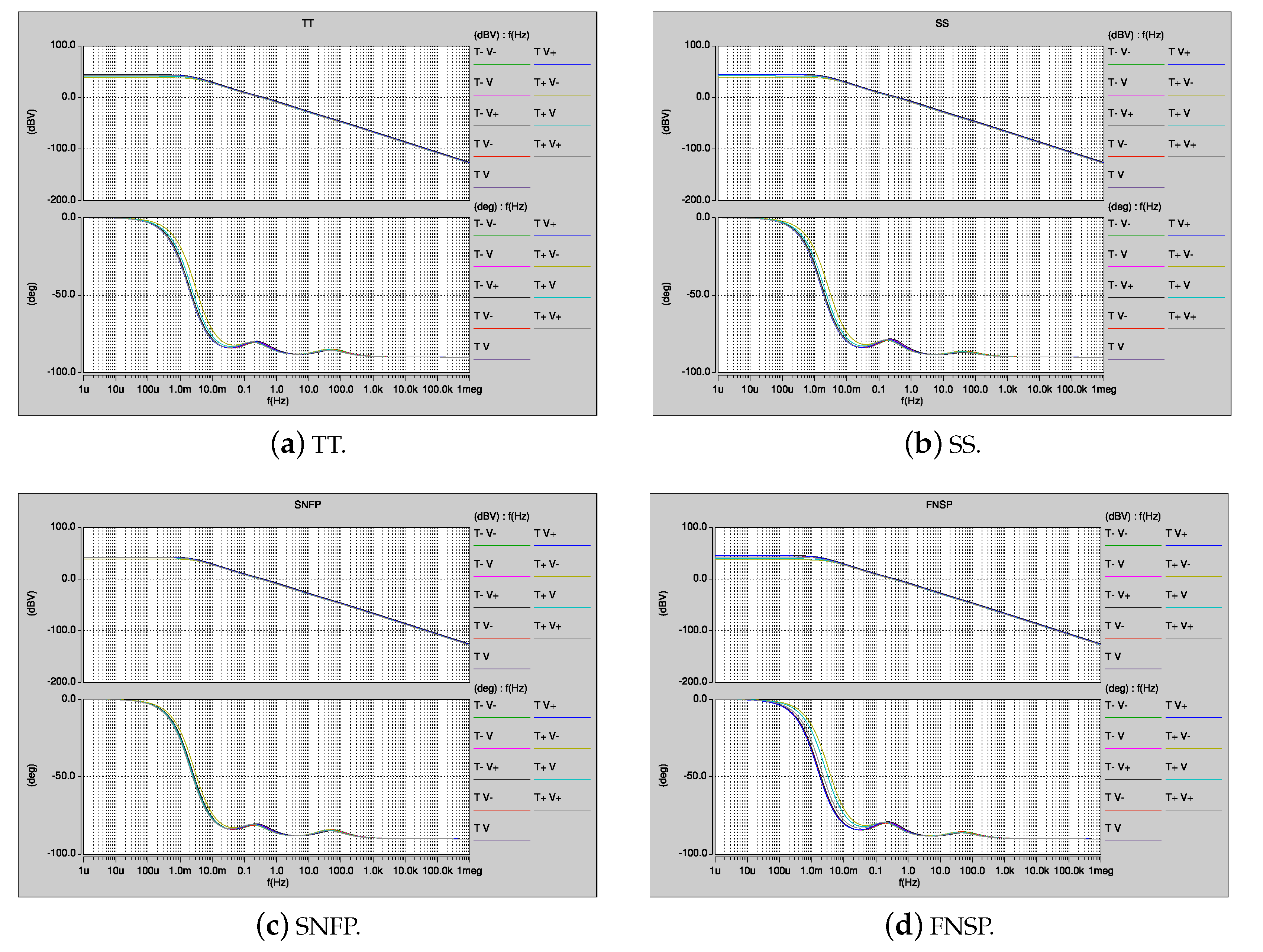
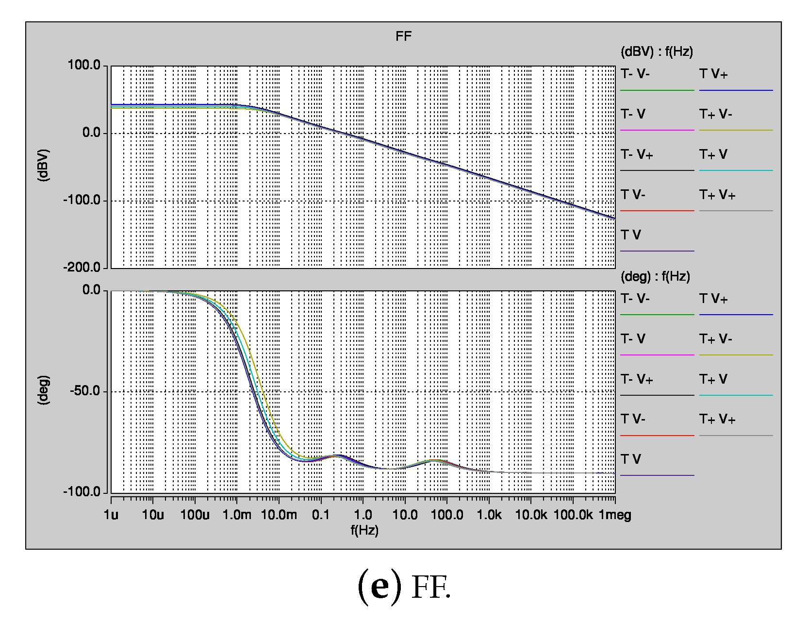
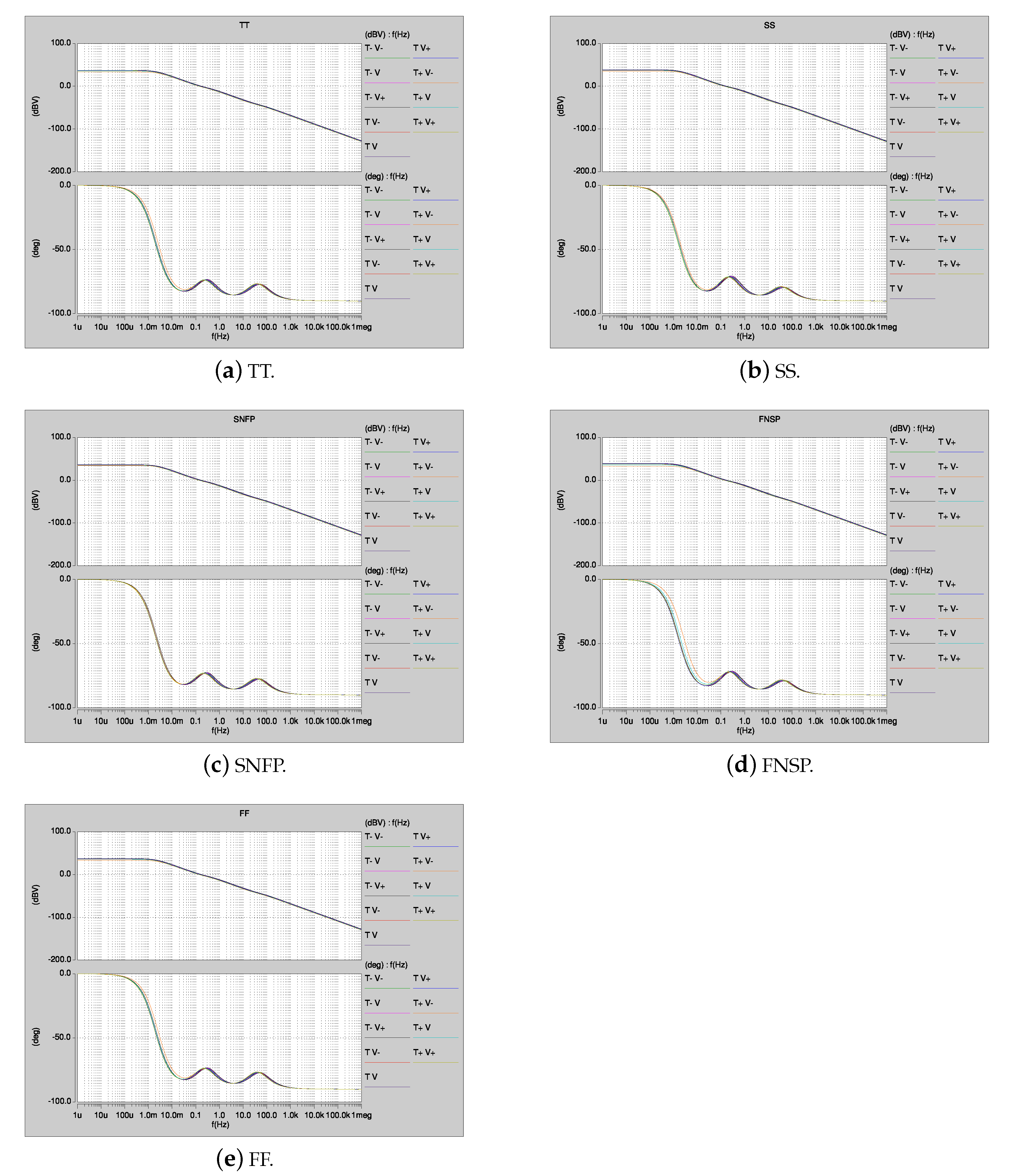
The robustness of the fractional-order integrator was verified by performing a PVT analysis in the five corners: typical–typical (TT), fast–fast (FF), slow–slow (SS), slowN–fastP (SNFP) and fastN–slowP (FNSP). These corner analyses were simulated for the three OTAs and their results are shown in Figure 10 for the differential pair, Figure 11 for the one-stage OTA and Figure 12 for the RFC OTA. For each corner, the voltage supply was varied by ±10%. Likewise, the temperature was varied with values of 20 (T−), 60 (T) and 120 (T+).

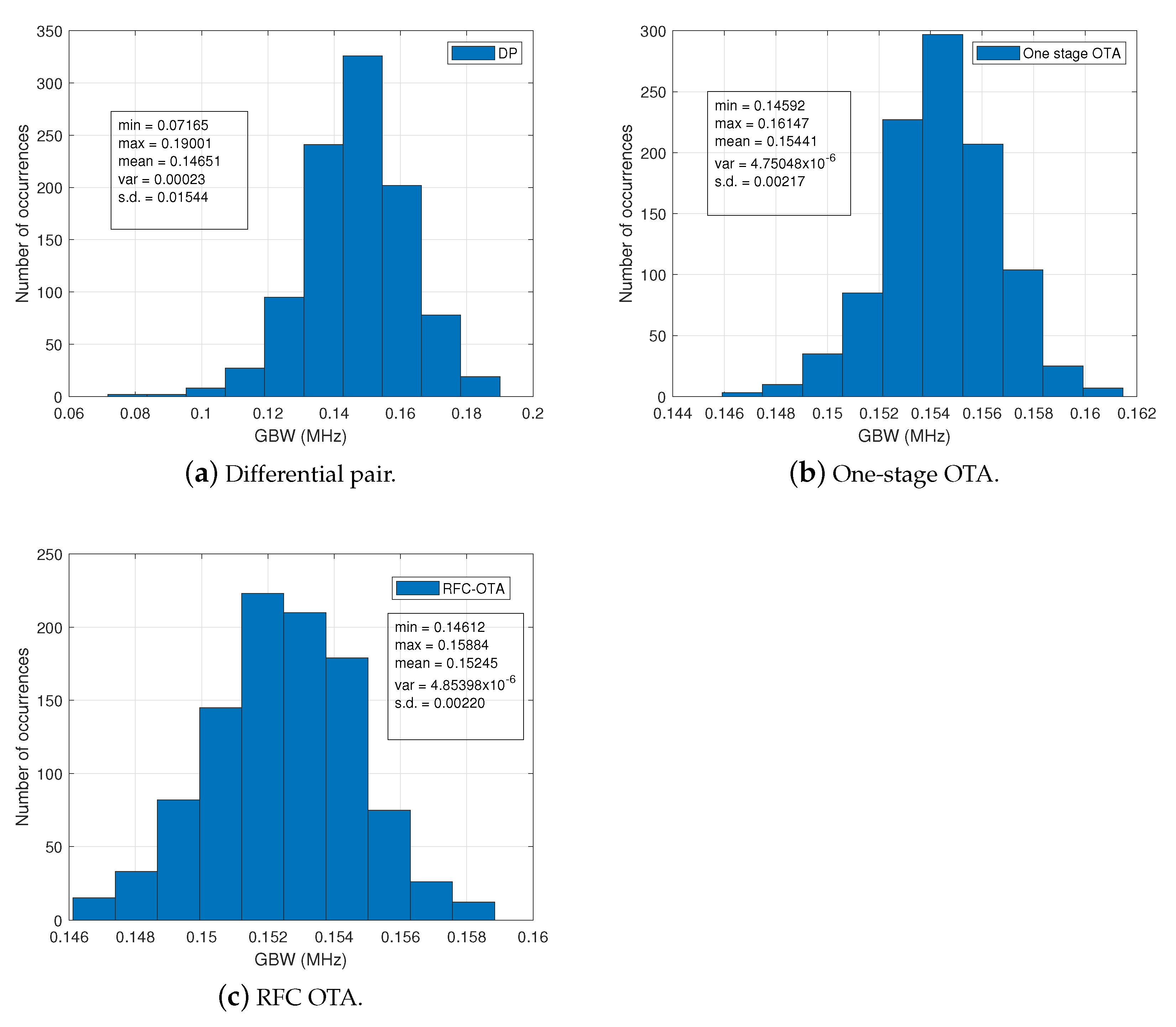
In addition to PVT analyses, a Monte Carlo analysis was performed to observe the variability due to matching conditions of the MOS transistors. This analysis was carried out assuming a deviation of 10% in the W’s and L’s of all MOS transistors. These two analyses were more than enough to appreciate the robustness of the CMOS design of the fractional-order integrator; therefore, it was used to design an FOCO. Figure 13 shows the histogram for each OTA topology for 1000 runs.

8.4. Fractional-Order Chaotic Oscillator Design Using OTAs

Once the fractional-order integrator was designed, the FOCO design was carried out; its OTA-based implementation is shown in Figure 14. It is noted the requirement of three fractional-order integrators (H(s)), five OTAs and one multiplier were required for its implementation. From (8), one can determine the value of the constants a, b and c. If the OTA has $g_m=500\mathsf{\mu }$A/V, the constant a is equal to $2.05\left(500\mathsf{\mu }\mathrm{A}/\mathrm{V}\right)=1025\mathsf{\mu }\mathrm{A}/\mathrm{V}$, $b=1.12\left(500\mathsf{\mu }\mathrm{A}/\mathrm{V}\right)=560\mathsf{\mu }\mathrm{A}/\mathrm{V}$ and $c=0.42\left(500\mathsf{\mu }\mathrm{A}/\mathrm{V}\right)=210\mathsf{\mu }\mathrm{A}/\mathrm{V}$. The three constants multiplying the convolution $X\left(s\right)\ast \left(X\right(s)$ in (8) leads to a transconductance value of $3\left(500\mathsf{\mu }\mathrm{A}/\mathrm{V}\right)=1500\mathsf{\mu }\mathrm{A}/\mathrm{V}$.

As mentioned above, the sizes of the OTAs were taken from the optimal solutions provided by the many-objective optimization with MOEA/D for five objectives. Finally, the portraits of the FOCO given in Figure 14 are shown in Figure 15, where the CMOS design was obtained using UMC technology at 180 nm. The bias was established at ±0.9. As can be seen, the MatLab simulation of the portraits of the FOCO shown in Figure 3 are in very good agreement with the portraits generated by the CMOS FOCO shown in Figure 15; therefore, we conclude confirming the suitability of performing many-objective optimization in the sizing of CMOS OTAs.

9. Conclusions

Sizing CMOS OTAs is a challenging task, mainly due to the large number of design variables and trade-offs among the target specifications. Fortunately, one can take advantage of applying metaheuristics to optimize such kinds of analog integrated circuits. In this manner, this paper shows the application of mono-, multi- and many-objective optimization algorithms to size three different CMOS OTA topologies. The many-objective optimization process was performed considering five different electrical characteristics taken as objective functions, namely, FoM, DC gain, power consumption, CMRR and total MOS area. The optimization results provided by the mono-, multi- and many-objective optimization algorithms to the three OTAs show that the many-objective metaheuristic not only found better sizing solutions in the main objective functions but also improved the trade-offs among the electrical characteristics, which lead to a more robust design. The robustness of the optimized OTAs was verified through PVT variation analyses and Monte Carlo simulations. That way, an optimized OTA was used to design a fractional-order integrator using OTA-C active filters. Finally, the CMOS OTA-based fractional-order integrator was used in the design of a CMOS fractional-order chaotic oscillator (FOCO). As a result of the optimization process, the MatLab simulations of the FOCO were in very good agreement with the CMOS design using UMC technology at 180 nm. This application of an optimized OTA in the design of an FOCO leads us to conclude that, although all metaheuristics are a good option to size CMOS OTAs, the application of many-objective optimization algorithms can provide much better results compared to mono- and multi-objective metaheuristics.

References

1. Tlelo-Cuautle, E.; Valencia-Ponce, M.A.; de la Fraga, L.G. Sizing CMOS amplifiers by PSO and MOL to improve DC operating point conditions. Electronics 2020, 9, 1027. [Google Scholar] [CrossRef]
2. Devi, S.; Guha, K.; Baishnab, K.L. Metaheuristic algorithms-based approach for optimal design of improvised fully differential amplifier for biomedical applications. In Proceedings of the 2021 Devices for Integrated Circuit (DevIC), Kalyani, Nadia, India, 19–20 May 2021; pp. 605–609. [Google Scholar]
3. Rashid, R.; Nambath, N. Hybrid Particle Swarm Optimization Algorithm for Area Minimization in 65 nm Technology. In Proceedings of the 2021 IEEE International Symposium on Circuits and Systems (ISCAS), Daegu, Korea, 22–28 May 2021; pp. 1–5. [Google Scholar]
4. Ben, Y.; Shi, G. Applying design equations in particle swarm optimization for auto-sizing of multi-stage opamps: An experimental study. Analog. Integr. Circuits Signal Process. 2020, 103, 117–130. [Google Scholar] [CrossRef]
5. Li, C.; You, F.; Yao, T.; Wang, J.; Shi, W.; Peng, J.; He, S. Simulated Annealing Particle Swarm Optimization for High-Efficiency Power Amplifier Design. IEEE Trans. Microw. Theory Tech. 2021, 69, 2494–2505. [Google Scholar] [CrossRef]
6. Lberni, A.; Marktani, M.A.; Ahaitouf, A.; Ahaitouf, A. Efficient butterfly inspired optimization algorithm for analog circuits design. Microelectron. J. 2021, 113, 105078. [Google Scholar] [CrossRef]
7. Kumar, R.; Talukdar, F.; Rajan, A.; Devi, A.; Raja, R. Parameter optimization of 5.5 GHz low noise amplifier using multi-objective Firefly Algorithm. Microsyst. Technol. 2020, 26, 3289–3297. [Google Scholar] [CrossRef]
8. Mostafa, S.S.; Horta, N.; Ravelo-Garcia, A.G.; Morgado-Dias, F. Analog active filter design using a multi objective genetic algorithm. AEU-Int. J. Electron. Commun. 2018, 93, 83–94. [Google Scholar] [CrossRef]
9. Papadimitriou, A.; Bucher, M. Multi-objective low-noise amplifier optimization using analytical model and genetic computation. Circuits Syst. Signal Process. 2017, 36, 4963–4993. [Google Scholar] [CrossRef]
10. Abi, S.; Bouyghf, H.; Benhala, B.; Raihani, A. An Optimal Design of a Short-Channel RF Low Noise Amplifier Using a Swarm Intelligence Technique. Embed. Syst. Artif. Intell. 2020, 1076, 143–153. [Google Scholar]
11. Nayak, B.; Choudhury, T.R.; Misra, B. Component value selection for active filters based on minimization of GSP and E12 compatible using Grey Wolf and Particle Swarm Optimization. AEU-Int. J. Electron. Commun. 2018, 87, 48–53. [Google Scholar] [CrossRef]
12. Dekimpe, R.; Bol, D. A Configurable ULP Instrumentation Amplifier with Pareto-Optimal Power-Noise Trade-Off Achieving 1.93 NEF in 65 nm CMOS. IEEE Trans. Circuits Syst. II Express Briefs 2021, 68, 2272–2276. [Google Scholar] [CrossRef]
13. Liao, T.; Zhang, L. Parasitic-aware GP-based many-objective sizing methodology for analog and RF integrated circuits. In Proceedings of the 2017 22nd Asia and South Pacific Design Automation Conference (ASP-DAC), Chiba, Japan, 16–19 January 2017; pp. 475–480. [Google Scholar]
14. Liao, T.; Zhang, L. Layout-dependent effects aware gm/iD-based many-objective sizing optimization for analog integrated circuits. In Proceedings of the 2018 IEEE International Symposium on Circuits and Systems (ISCAS), Florence, Italy, 27–30 May 2018; pp. 1–5. [Google Scholar]
15. Martins, R.; Lourenço, N.; Horta, N.; Yin, J.; Mak, P.I.; Martins, R.P. Many-objective sizing optimization of a class-C/D VCO for ultralow-power IoT and ultralow-phase-noise cellular applications. IEEE Trans. Very Large Scale Integr. (VLSI) Syst. 2018, 27, 69–82. [Google Scholar] [CrossRef]
16. Touloupas, K.; Sotiriadis, P.P. Analog and RF Circuit Constrained Optimization Using Multi-Objective Evolutionary Algorithms. In Proceedings of the 2021 IEEE 12th Latin America Symposium on Circuits and System (LASCAS), Arequipa, Peru, 21–24 February 2021; pp. 1–4. [Google Scholar]
17. Ishibuchi, H.; Tsukamoto, N.; Nojima, Y. Evolutionary many-objective optimization: A short review. In Proceedings of the 2008 IEEE Congress on Evolutionary Computation (IEEE World Congress on Computational Intelligence), Hong Kong, China, 1–6 June 2008; pp. 2419–2426. [Google Scholar]
18. Liang, Z.; Liang, W.; Wang, Z.; Ma, X.; Liu, L.; Zhu, Z. Multiobjective Evolutionary Multitasking With Two-Stage Adaptive Knowledge Transfer Based on Population Distribution. IEEE Trans. Syst. Man Cybern. Syst. 2021, 1–13. [Google Scholar] [CrossRef]
19. Yosefi, G. A special technique for Recycling Folded Cascode OTA to improve DC gain, bandwidth, CMRR and PSRR in 90 nm CMOS process. Ain Shams Eng. J. 2020, 11, 329–342. [Google Scholar] [CrossRef]
20. Liao, P.H.; Hwang, Y.S.; Chen, J.J.; Ku, Y.; Wang, S.F. A new low-voltage operational transconductance amplifier with push-pull CMFB scheme for low-pass filter applications. AEU-Int. J. Electron. Commun. 2020, 123, 153298. [Google Scholar] [CrossRef]
21. Geiger, R.L.; Sanchez-Sinencio, E. Active filter design using operational transconductance amplifiers: A tutorial. IEEE Circuits Devices Mag. 1985, 1, 20–32. [Google Scholar] [CrossRef]
22. Somal, S.; Sharma, T.; Mehra, K. Design of Ultra-Low Power OTA Based on Subthreshold Operation with High Gain, Large Transconductance and Small Area. In Intelligent Communication and Automation Systems; CRC Press: London, UK, 2021; pp. 139–148. [Google Scholar]
23. Renteria-Pinon, M.; Ramirez-Angulo, J.; Diaz-Sanchez, A. Simple scheme for the implementation of low voltage fully differential amplifiers without output common-mode feedback network. J. Low Power Electron. Appl. 2020, 10, 34. [Google Scholar] [CrossRef]
24. Konal, M.; Kacar, F. Extended Bandwidth Method on Symmetrical OTA and Filter Application. Inf. MIDEM 2021, 51, 100. [Google Scholar]
25. Mathad, R.S.; Bhat, K. A Multipurpose Noise and Vibration Data Acquisition System using OTA Amplifiers and Filters. In Proceedings of the 2021 2nd International Conference for Emerging Technology (INCET), Belagavi, India, 21–23 May 2021; pp. 1–4. [Google Scholar]
26. Singh, B.K.; Shankar, G.; Jain, B.B. An Overview on Low Voltage Low Power Operational Transconductance Amplifier (OTA) for Biomedical Application. Int. J. Eng. Trends Appl. (IJETA) 2021, 8, 1–5. [Google Scholar]
27. Rawat, A.S.; Rajendran, J.; Ramiah, H.; Rana, A.; Jugran, S. 88-dB Gain with Improved Phase Margin Telescopic Cascode OTA for RF-IoT Applications. In Proceedings of Integrated Intelligence Enable Networks and Computing; Springer: Singapore, 2021; pp. 413–420. [Google Scholar]
28. Feizbakhsh, S.V.; Yosefi, G. An enhanced fast slew rate recycling folded cascode Op-Amp with general improvement in 180 nm CMOS process. AEU-Int. J. Electron. Commun. 2019, 101, 200–217. [Google Scholar] [CrossRef]
29. Venishetty, S.R.; Sundaram, K. Design and analysis of modified recycling folded cascode amplifier with improved transconductance and slew rate. Eng. Appl. Sci. Res. 2020, 47, 430–438. [Google Scholar]
30. Carbajal-Gomez, V.H.; Tlelo-Cuautle, E.; Muñoz-Pacheco, J.M.; de la Fraga, L.G.; Sanchez-Lopez, C.; Fernandez-Fernandez, F.V. Optimization and CMOS design of chaotic oscillators robust to PVT variations. Integration 2019, 65, 32–42. [Google Scholar] [CrossRef]
31. Savic, D. Single-Objective vs. Multiobjective Optimisation for Integrated Decision Support. In Proceedings of the 1st International Congress on Environmental Modelling and Software, Lugano, Switzerland, 24–27 June 2002. [Google Scholar]
32. Wang, D.; Tan, D.; Liu, L. Particle swarm optimization algorithm: An overview. Soft Comput. 2018, 22, 387–408. [Google Scholar] [CrossRef]
33. Kaveh, A. Advances in Metaheuristic Algorithms for Optimal Design of Structures; Springer: Cham, Switzerland, 2014. [Google Scholar]
34. Pedersen, M.E.H.; Chipperfield, A.J. Simplifying particle swarm optimization. Appl. Soft Comput. 2010, 10, 618–628. [Google Scholar] [CrossRef]
35. Mohanty, P.; Sahu, R.K.; Panda, S. A novel hybrid many optimizing liaisons gravitational search algorithm approach for AGC of power systems. Automatika 2020, 61, 158–178. [Google Scholar] [CrossRef]
36. Pant, M.; Zaheer, H.; Garcia-Hernandez, L.; Abraham, A. Differential Evolution: A review of more than two decades of research. Eng. Appl. Artif. Intell. 2020, 90, 103479. [Google Scholar]
37. Singh, A.; Kumar, S. Differential evolution: An overview. In Proceedings of Fifth International Conference on Soft Computing for Problem Solving; Springer: Singapore, 2016; pp. 209–217. [Google Scholar]
38. Deb, K.; Pratap, A.; Agarwal, S.; Meyarivan, T. A fast and elitist multiobjective genetic algorithm: NSGA-II. IEEE Trans. Evol. Comput. 2002, 6, 182–197. [Google Scholar] [CrossRef] [Green Version]
39. Goldenberg, D.E. Genetic Algorithms in Search, Optimization and Machine Learning; Addison-Wesley Professional: Boston, MA, USA, 1989. [Google Scholar]
40. Zhang, Q.; Li, H. MOEA/D: A multiobjective evolutionary algorithm based on decomposition. IEEE Trans. Evol. Comput. 2007, 11, 712–731. [Google Scholar] [CrossRef]
41. Purshouse, R.C.; Fleming, P.J. Evolutionary many-objective optimisation: An exploratory analysis. In Proceedings of the 2003 Congress on Evolutionary Computation, CEC’03, Canberra, ACT, Australia,, 8–12 December 2003; Volume 3, pp. 2066–2073. [Google Scholar]
42. Deb, K.; Jain, H. An evolutionary many-objective optimization algorithm using reference-point-based nondominated sorting approach, part I: Solving problems with box constraints. IEEE Trans. Evol. Comput. 2013, 18, 577–601. [Google Scholar] [CrossRef]
43. Mkaouer, W.; Kessentini, M.; Shaout, A.; Koligheu, P.; Bechikh, S.; Deb, K.; Ouni, A. Many-objective software remodularization using NSGA-III. ACM Trans. Softw. Eng. Methodol. (TOSEM) 2015, 24, 1–45. [Google Scholar] [CrossRef]
44. Asafuddoula, M.; Ray, T.; Sarker, R. A decomposition-based evolutionary algorithm for many objective optimization. IEEE Trans. Evol. Comput. 2014, 19, 445–460. [Google Scholar] [CrossRef]
45. Gómez, R.H.; Coello, C.A.C. MOMBI: A new metaheuristic for many-objective optimization based on the R2 indicator. In Proceedings of the 2013 IEEE Congress on Evolutionary Computation, Cancun, Mexico, 20–23 June 2013; pp. 2488–2495. [Google Scholar]
46. EMO Project. Available online: http://computacion.cs.cinvestav.mx/~rhernandez/ (accessed on 16 August 2017).
47. Pandey, A.; Baghel, R.; Singh, R. Analysis and circuit realization of a new autonomous chaotic system. Int. J. Electron. Commun. Eng. 2012, 5, 487–495. [Google Scholar]
48. Tlelo-Cuautle, E.; Pano-Azucena, A.D.; Guillén-Fernández, O.; Silva-Juárez, A. Analog/Digital Implementation of Fractional Order Chaotic Circuits and Applications; Springer: Cham, Switzerland, 2020. [Google Scholar]
49. Valencia-Ponce, M.A.; Castañeda-Aviña, P.R.; Tlelo-Cuautle, E.; Carbajal-Gómez, V.H.; González-Díaz, V.R.; Sandoval-Ibarra, Y.; Nuñez-Perez, J.C. CMOS OTA-Based Filters for Designing Fractional-Order Chaotic Oscillators. Fractal Fract. 2021, 5, 122. [Google Scholar] [CrossRef]
50. Pantoja, L.F.M.; Sánchez, A.D.; Pérez, J.M.R. A new Tunable Pseudo-Resistor for Extremely/Ultra Low Frequency applications. In Proceedings of the 2019 16th International Conference on Electrical Engineering, Computing Science and Automatic Control (CCE), Mexico City, Mexico, 11–13 September 2019; pp. 1–5. [Google Scholar]
51. de la Fraga, L.G.; Tlelo-Cuautle, E. Linearizing the Transconductance of an OTA Through the Optimal Sizing by Applying NSGA-II. In Proceedings of the 2018 15th International Conference on Synthesis, Modeling, Analysis and Simulation Methods and Applications to Circuit Design (SMACD), Prague, Czech Republic, 2–5 July 2018; pp. 1–9. [Google Scholar]
Figure 1. CMOS OTAs with source degeneration to improve linearity and allow g m to be programmed.
Electronics 10 03148 g001
Figure 2. P-type MOS transistors used to design the variable resistors shown in Figure 1.
Electronics 10 03148 g002
Figure 3. Portraits of the attractors of the FOCO given in (8).
Electronics 10 03148 g003
Figure 4. Block design of the FOCO given in (8). H ( s ) denotes the fractional-order integrator H ( s ) = 1 / s 0.9 , approximated by (9).
Electronics 10 03148 g004
Figure 5. Fully differential four-quadrant multiplier taken from [49].
Electronics 10 03148 g005
Figure 6. OTA-based active filters to design the biquadratic and first-order low pass filters.
Electronics 10 03148 g006
Figure 7. Pseudo-resistor taken from [50].
Electronics 10 03148 g007
Figure 8. Proposed OTA design for 1 s 0.9 using a biquadratic and a low-pass filter.
Electronics 10 03148 g008
Figure 9. Frequency response of the fractional-order integrator, considering ideal transfer function approximation in MatLab, macro-modeling and HSPICE simulation using the CMOS differential pair (DP), one-stage and RFC OTAs.
Electronics 10 03148 g009
Figure 10. PVT simulations of the CMOS fractional-order integrator given in Figure 8 using the differential pair amplifier shown in Figure 1.
Electronics 10 03148 g010aElectronics 10 03148 g010b
Figure 11. PVT simulations of the CMOS fractional-order integrator given in Figure 8 using the one-stage OTA given in Figure 1.
Electronics 10 03148 g011aElectronics 10 03148 g011b
Figure 12. PVT simulations of the CMOS fractional-order integrator given in Figure 8 using the RFC OTA given in Figure 1.
Electronics 10 03148 g012
Figure 13. Monte Carlo simulation.
Electronics 10 03148 g013
Figure 14. OTA-based implementation of the FOCO given in (8). The multiplier is designed from Figure 5 and the fractional order integrator H(s) is designed as detailed in Section 8.2.
Electronics 10 03148 g014
Figure 15. HSPICE portraits of the proposed CMOS OTA-based FOCO from Figure 14.
Electronics 10 03148 g015aElectronics 10 03148 g015b