Deep Time-Series Clustering: A Review

Abstract

We present a comprehensive, detailed review of time-series data analysis, with emphasis on deep time-series clustering (DTSC), and a case study in the context of movement behavior clustering utilizing the deep clustering method. Specifically, we modified the DCAE architectures to suit time-series data at the time of our prior deep clustering work. Lately, several works have been carried out on deep clustering of time-series data. We also review these works and identify state-of-the-art, as well as present an outlook on this important field of DTSC from five important perspectives.

1. Introduction

Recent advances in time-series clustering have shown great success in a range of fields, including networks and systems, meteorology, social media, behavior analysis, trajectory data, biological science, and finance. Extracting useful structures from large volumes of data requires interdisciplinary research involving several domains such as statistics, machine learning, data visualization, pattern recognition, and high-performance computing [1]. Despite the progress made in time-series data clustering, the presence of noise, high dimensionality, and high feature correlation pose challenges in designing effective and efficient clustering algorithms. Traditional algorithms display limited performance with the increase in data dimensionality. Variants of deep learning methods have shown a robust ability in representation learning, finding the most success in supervised learning. We developed deep learning-based methods for clustering analysis based on deep learning’s ability to deliver high-level representations from data. We have proposed deep cluster, a clustering approach embedded in a deep convolutional auto-encoder (DCAE), consisting of clustering and reconstruction objective functions. Its results on different datasets have shown the ability of deep clustering models to substantially outperform other methods in terms of clustering quality. We published this work in ICIP 2018 [2]. At that time, we also applied these deep clustering methods to time-series data in the experiment reported here. Specifically, we modified the DCAE architectures to suit time-series data; see Section 5 for details. Since 2018, several works have been reported on deep clustering of time-series data. We also review these works in this paper and identify the state-of-the-art and present an outlook on this important field of deep time-series clustering (DTSC).

The paper is organized as follows. First, Section 2 describes the methodology used to collect related research papers and the scope of the literature. A detailed review of conventional time-series analysis is provided in Section 4. In Section 5, we introduce the use of DTSC and its methodology to learn and cluster temporal features from time-series data, discussing its challenges, opportunities, and future directions. Finally, concluding remarks and summary are provided in Section 7.

2. Methodology

2.1. Review Search Methodology

A variety of concepts and methods are involved in clustering time-series data. Our search methodology was to collect, study and analyze many papers in the field of time-series analysis. In our search of the literature, we started by looking at each individual journal and conference in the relevant communities. We performed a keyword search, e.g., ‘time-series data’, ‘similarity measures’, ‘feature extraction’, ‘clustering’, ‘deep neural network’, or ‘deep learning’.

2.2. Review Scope

To fulfill the scope of our survey, we have selected papers that focus on time-series data and clustering algorithms. We found and collected many papers to include in our review of deep time-series clustering. We pay attention to time series similarity measures and feature extraction, clustering algorithms, and deep time-series clustering.

2.3. Review Structure

Figure 1 shows the review framework, which is derived from the main process of the survey methods. We start with time series data structures, where we provide a general classification for time series data. All data structures, as described in Section 3, refer to the main definition of time series data, and this section answers questions such as how time series data structures are different, along with providing some examples of this kind of data.

Section 4 reviews the conventional time series analysis. In Section 4.1, we discuss similarity measures and feature extraction, which are important for time series data as, usually, the quality of analysis techniques (such as conventional clustering) are significantly influenced by its selection. Moreover, in this section, we show how these techniques, along with clustering techniques, have been adapted to gain knowledge from the data. In Section 4.2, we provide a comprehensive explanation for popular conventional clustering algorithms that have been used in the surveyed papers and how they are used with time series data.

In Section 5, we introduce the use of deep clustering methodology to learn and cluster temporal features from accelerometer data for the clustering of animal behaviors, applying the deep clustering method to real-world data; namely, the Imperial Cormorant bird dataset (ICBD) from the Biosciences department at Swansea University. Other recent works are subsequently discussed in Section 6, describing the challenges of DTSC, opportunities, and future directions.

3. Time-Series Data Types

Time-series data is an umbrella term for many different data with an associated time component. It is defined as an ordered collection of observations or sequences of data points made over time, usually at uniform time intervals. In order to understand the complexity of time-series and explore the underlying processes, the processing and analysis of such data require particular supporting tasks and methods. Here, we classify time-series data into four categories, subsumed under the concepts of univariate, multivariate, tensor fields, and multifields. Hotz et al. [3] discuss the complex structure of scientific data and provide a clear definition of a multifield. The four types, or categories, are generalized to include many related subtypes of time-series data in order to achieve a comprehensive classification for said data.

3.1. Univariate

The univariate time-series is a sequence that contains only one data value per temporal primitive [1,4]. It is a field of a single variable captured or observed through time. The temperature in a city spanning a period of time is a clear example of this type of data.

3.2. Multivariate

Multivariate time-series is a set of time-series that have the same timestamps [1,4]. This type of time-series data is an array of variables or numbers at each point in time and can be a collection of multiple univariates captured through time, such as temperature and pressure readings, or associative multivariate, such as 3D acceleration measured from a tri-axial accelerometer, where each component of the multivariate has the same units and sensor source. As time-series data is an ordered collection of observations or a sequence of data points made over time, this special type of multivariate time-series data is relevant in many fields including biology, medicine, finance and animation. Multivariate time-series data have been used in manufacturing systems and predictive maintenance [5,6]. Time-series data obtained from gene expression measurement [7,8,9], for instance, can be used by biologists to understand the correlation between types of genes, analyze gene interactions, and compare regulatory behaviors for genes of interest. Medical experts also utilize time-series data from blood pressure measurements [10] to understand and deal with cases such as monitoring illness progression, and understanding ecological and behavioral processes related to a disease, which may lead to improved diagnoses. Furthermore, time-series data such as that obtained from sampled transactions over a period of time [11,12,13], stock markets [14,15], and international financial markets [16,17] can be used in the financial field and are analyzed to understand and forecast market conditions. It is useful to find correlations between the data and test hypotheses about the market, as this helps in making correct decisions at the appropriate time under changing business and economic circumstances. A multivariate can also present time-series data obtained from various data sets including metadata, e.g., patient records [18,19], employment records [20,21], and social networks [22].

3.3. Tensor Fields

These comprise an array of data arranged on a regular grid with a variable number of axes [23]. They can be described as a quantity associated with each point in space-time and have also been extended to functions or distributions linked to points in space-time [3]. Dealing with spatio-temporal data, this type of time-series data is generalized to include many related subtypes: time-series of graphs and networks, time-series of spatial positions of moving objects, and time-series of spatial configurations/distributions.

3.3.1. Time-Series of Graph and Network

Time-series data in the form of networks consist of associated attributes such as nodes and edges that reflect different kinds of behavior over time. Node or edge attributes of dynamic graphs can be introduced as time-series. This kind of time-series data helps with understanding different temporal patterns and evaluation of the network dynamics in general [24,25,26,27,28]. For example, a computer typically consists of a large number of sensors that produce massive quantities of time-series data, such as CPU load, memory usage, network load, and data center chiller sensor. Anaylsis and visualization approaches exist that help to improve the understanding of how machines are used in practice and analyze the performance and behaviors of such systems [29,30,31,32,33,34,35]. Indeed, analyzing this data can help users and experts understand and evaluate the network dynamics.

3.3.2. Time-Series of Spatial Positions of Moving Objects

Spatial positions of moving objects data with an associated time component classifies as trajectory data. It presents different places over time, providing a clear idea of spatio-temporal changes. The process and analysis of time-series data are important procedures for understanding the characteristics of the data and obtaining meaningful statistics, which aid the exploration of the underlying processes, analysis, tracking, and representation of this type of data in order to understand and recognize the mobility of a diverse array of moving objects, such as vehicles [36,37,38,39,40,41,42,43], and aircraft [38,39], which aid path discovery, movement analysis, and location prediction.

3.3.3. Time-Series of Spatial Configurations and Distributions

Being able to extract useful insights from time-series of spatial distributions and configurations has become increasingly important due to significant growth in data science and rapid advancement in many technologies. In our research, we consider discovering behavioral patterns and finding interesting events that might take place in certain municipalities [44] and public or business sectors as spatial configurations and distributions. This identification of regular configurations and distributions over time is represented by a total number of events and behaviors extracted from a chosen spatial scale. Personal mobility behaviors and movement patterns [45,46,47,48,49,50,51,52,53], behaviors of animals [54,55], pattern changes in climate (weather) and the ozone layer [53,56,57,58,59,60,61,62], and behavior capture data made through time at often uniform time intervals [63,64,65,66,67,68] can be regarded as instances of this type of data that take place in specific spatial identification.

3.4. Multifield

This kind of data, defined as a set of fields, provides enough flexibility to capture most types of compound datasets that occur in practice [3]. Combining multiple modality sensors such as gyroscopes, magnetometers and accelerometers with other environmental sensors is an example of this data type.

4. Conventional Time-Series Analysis

For time-series data, the presence of noise, high dimensionality, and high feature correlation pose challenges for designing effective and efficient clustering algorithms compared to data without a temporal component [1,69]. Analyzing time-series data is nontrivial and can even vary over time due to complex interrelations between time-series variables. Xing et al. [70] describe three significant challenges for time-series analysis. First, many methods can only take input data as a vector of features. Unfortunately, there are no explicit features in sequence data. Second, feature selection is not easy because the dimensionality of the feature space can be high and computation can be costly. Third, since there are no explicit features in the raw data, building a partitioning task is burdensome in some applications. Therefore, efficiently handling the raw data in time-series is difficult without using similarity measures and feature extraction to reduce dimensionality and provide representative features of such data. These challenges led to the conventional time-series analysis pipeline, which consists of three different perspectives, these being time-series data, similarity measures and feature extraction, and time-series clustering (see Figure 2).

4.1. Similarity Measures and Feature Extraction

Large time-series data require adequate pre-processing to gain an appropriate approximation of the underlying data representation. The aim is to generate a higher-level abstraction that represents the data while preserving the shape characteristics of the original data during dimensionality reduction. There are several dimensionality reduction techniques specifically designed for time-series that exploit the frequential content of the signal and its usual sparseness in the frequency space [71]. In general terms, choosing a distance measure is important and assists in dealing with outliers, amplitude differences, and time axis distortion. Furthermore, selecting important features in the data requires sufficient communication of knowledge from domain experts. Thus, the quality of clustering approaches is significantly affected by the choice of similarity measures and feature extraction techniques to obtain the relevant knowledge from the data.

Computing the similarity between two data objects is considered one of the main differences between clustering of temporal and non-temporal data [72,73]. The unique characteristics of time-series data such as noise, including outliers and shifts, and the varying length of time-series has made similarity measures one of the main challenges for clustering of time-series data [74]. The greatest challenge lies in replacing the distance/similarity measure for static data with a suitable one for time-series data, because it may be scaled and translated differently on both the temporal and behavioral dimensions [69,75]. Therefore, modifying distance functions to suit the characteristics of time-series data has become essential when developing a clustering method for time-series data. Batóg et al. [76] applied cluster analysis to identify the level of business activity convergence, based on an adaptive dissimilarity index covering both proximity on values and on behavior, Euclidean distance and concordance measure. They used two measures of similarity of time series: the first-order temporal correlation coefficient and Euclidean distance for standardized values. Petitjean et al. [77] also introduced a kDBA method that combines k-means and dynamic time warping for better alignment. Moreover, Yang et al. [78] presented the K-Spectral Centroid (K-SC) method, using an invariant similarity metric to reveal the temporal dynamics. Lastly, Paparrizos et al. [79] developed a k-Shape method whereby the shapes of the time-series are considered by applying cross-correlation measures. However, these methods are usually sensitive to noise and outliers because all time points are considered [80].

The quality of clustering methods is significantly affected by the choice of feature extraction technique. Guo et al. [81] proposed a feature-based approach to time-series clustering by applying independent component analysis to convert the raw time-series into a lower-dimensional feature vector and then further applying k-means clustering on the extracted features. In addition, Zakaria et al. [82] employed u-shapelet algorithms to learn local patterns in a time-series, as they are highly predictive when performing clustering. Popescu [83] used some statistical models such as ARIMA to analyze and forecast road traffic accidents. They stated that ARIMA models and the attractive features of the Box–Jenkins approach can provide an adequate description of the time-series data and can provide answers to relevant questions about the data. Other recent advances in feature extraction have efficiently supported clustering tasks, where linear [84,85,86,87] and non-linear [88,89,90,91] methods have been adopted to transform the original time-series data into representative features, allowing unsupervised clustering methods to deal with features instead of raw data.

The below discussion about the types of methods provides a review of popular similarity measures and feature extraction techniques along with works that have been adopted in time-series data mining.

4.1.1. Raw Data Similarity

Most mining approaches utilize the concept of the similarity between a pair of time-series. Similarity measures must be chosen when dealing with time-series data in order to take into account outliers, different amplitude, and time axis distortion. When dealing with time-series data, efficiency and effectiveness are the main targets of representation methods and similarity measures [92]. Tornai et al. [93] argue that the distance between two sequences as a measurement plays an important role in the quality of clustering algorithms. The accuracy of such algorithms can be significantly impacted by the choice of similarity measures. Yahyaoui et al. [94] and Wang et al. [92] presented a comprehensive review of time-series measures, classifying them into four major categories: lock-step measures (e.g., Euclidean distance and Manhattan distance), elastic measures (e.g., longest common subsequence (LCS) and dynamic time warping (DTW)), pattern-based measures (e.g., spatial assembling distance (SpADe)), and threshold-based measures (e.g., threshold query based similarity search (TQuEST)). The types of methods, discussed below, are intended to provide a review of popular similarity measures.

Euclidean distance (ED): is a commonly used metric for time-series. It is defined between two time-series X and Y having length L; therefore, the Euclidean distance, between each pair of corresponding points X and Y, is the square root of the sum of the squared differences [95]. Thus, the two time-series being compared must have the same length, and the computational cost is linear in terms of temporal sequence length [96]. Along the horizontal axis, the distance between the two time-series is calculated by matching the corresponding points [97]. The Euclidean distance metric is very sensitive to distortion and noise [70], and is not able to handle one of the elements being compressed or stretched [55]. This approach is therefore unreliable, especially when computing similarity between time-series with different time durations [98].

Dynamic Time Warping (DTW): is proposed to overcome some Euclidean distance limitations such as non-linear distortions. In DTW, the two time-series do not have to be the same length, and the idea is to align (warp) the series before computing the distance [70]. However, two temporal points with completely different local structures might be mistakenly matched by DTW. This issue can be addressed by improving the alignment algorithm, e.g., shape dynamic time warping which considers point-wise local structural information [99].

Due to its quadratic time complexity, DTW does not scale well when dealing with large datasets. Despite this, it is widely used in various applications, such as in bioinformatics, finance and medicine [100]. DTW has several local constraints, namely boundary, monotonicity and continuity constraints [98]. Common misunderstandings about DTW include conceptions that it is too slow to be useful and that the warping window size does not matter much; Wang et al. [92] and Mueen et al. [101] have attempted to correct these notions. Kotas et al. [102] have reformulated the matrix of the alignment costs, which led to a major increase in the noise reduction capability. Other surveys review distance measures such as Euclidean Distance (ED) [103], Dynamic Time Warping (DTW) [104,105], and distance based on Longest Common Subsequence (LCS) [92,106].

Correlation: is a mathematical operation widely used to describe how two or more variables fluctuate together. Different types of correlation can be found by considering the level of measurement for each variable. Distance correlation can be used as a distance measure between two variables that are not necessarily of equal dimension. In time-series data, it is used to detect a known waveform in random noise. Unlike DTW and LCS, correlation also offers a linear complexity frequency space implementation in signal processing [55,107].

Cross-correlation: is the correlation between two signals that shape a new signal, and its peaks can indicate the similarity between the original signals; it is used as a distance metric [74]. However, cross-correlation can be carried out more efficiently in the frequency domain [55,87,107]. Autocorrelation occurs when the signal is correlated with itself, which is useful for finding repeating patterns [55]. Cross-correlation might be a slow operation in time-series space, but it corresponds to point-wise multiplication in frequency space [55]. It is also considered the best distance measure to detect a known waveform in random noise [55]. When processing the signal, the correlation has a linear complexity frequency space implementation [55,87], which cannot be achieved by DTW.

4.1.2. Features Extraction

Feature extraction is a form of dimension reduction which helps to lower the computational cost of dealing with high-dimensional data and achieve higher accuracy of clustering [108]. Matching features from time-series data, should be extracted before applying learning algorithms to the vector of extracted features. Several feature-based techniques have been proposed to represent features with low dimensionality for time-series data. Wang et al. [92] list several methods for reducing time-series dimensionality as feature extraction; including Discrete Fourier Transform (DFT), Discrete Wavelet Transform (DWT), Discrete Cosine Transform (DCT), Single Value Decomposition (SVD), Adaptive Piecewise Constant Approximation (APCA), Piecewise Aggregate Approximation (PAA), Chebyshev polynomials (CHEB), and Symbolic Aggregate approXimation (SAX).

Principal Component Analysis (PCA), as an eigenvalue method, is a technique that transforms the original time-series data into low-dimensional features. As a feature extraction method, PCA is effectively applied to time-series data [109,110,111,112]. It transforms data into a new set of variables whose elements are mutually uncorrelated, thus learning a representation of data that has lower dimensionality than the original input. PCA is a linear dimensionality reduction technique, and has been used as an effective dimensionality reduction method that eliminates the least significant information in the data and preserves the most significant. The papers [13,26,42,56,59,63,68,113] use PCA to reduce high-dimensional data and analyze the similarity of time-series data.

Multidimensional Scaling (MDS): is a very popular non-linear dimensionality reduction technique that is useful for effectively representing high-dimensionality data in lower dimensional space [8,20,26,28,29,35,50,53,56]. It struggles, however, to separate k-means clusters [56]. Jeong et al. [8] use MDS to gain a better understanding of gene interactions and regulatory behaviors. Thus, two different MDS representations are considered with respect to time-series data. One shows local differences among genes in the same cluster group, while the other shows global differences among all genes in all the clusters. It is also used to reveal the distributions of the time-series data, helping to understand the relations among time-series [20].

K-grams: Transforming time-series data into a set of features cannot fully capture the sequential nature of series. K-gram is an example of a feature-based technique that aims to maintain the order of elements in series using short sequence segments of k consecutive symbols [94]. K-grams [114] represent a feature vector of symbolic sequences of K-grams in time-series data. Given a set of K-grams, this feature vector can represent the frequency of the K-grams (i.e., how often a K-gram appears in a sequence).

Discrete Fourier Transform (DFT): is one of the most common transformation methods [115]. It has been used to transform original time-series data into low-dimensionality time-frequency characteristics and index them to obtain an effective similarity search [116]. DFT is used to perform dimensionality reduction and extract features into an index used for similarity searching. This technique is continually under improvement and some of its limitations have been overcome [103,117,118].

Discrete Wavelet Transform (DWT): has also been used as a technique to transform original time-series and obtain low-dimensional features that efficiently represent the original time-series data [93,119]. Chan et al. [120] use Haar Wavelet Transform for time-series indexing, which shows the technique’s effectiveness with regard to the decomposition and reconstruction of time-series. With a large set of time-series data, analysis tasks face certain challenges in defining matching features; therefore, taking advantage of wavelet decomposition to reduce the dimensionality of data is beneficial [121]. The analysis task can be accurately performed utilizing the discrete wavelet transform technique [122].

Shapelets: Discretization is often required when applying feature-extraction techniques in time-series data, but it can cause information loss [70]. To address this, Ye et al. [123] introduce time-series shapelets, which can be directly applied to time-series. This technique is based on comparing the subsection of shapes (shapelets) instead of comparing the whole time-series sequences to measure the similarity. A binary decision maker decides whether each new sequence belongs to a class or not. The shapelet classifier has some limitations with a multi-class problem, and to overcome this issue, Ye et al. [123] use the shapelet classifier as a decision tree. Xing et al. [124] show that early classification can be efficiently achieved by extracting the local shapelets features.

4.2. Conventional Clustering Algorithms

Clustering is widely used as an unsupervised learning method. The aim of time-series clustering is to define a grouped structure of similar objects in unlabeled data based on their similar features. Due to the unique structure of time-series data (e.g., high dimensionality, noise, and high feature correlation), clustering time-series differs from traditional clustering, consequently, several algorithms have been improved to deal with time-series. Most works involving the clustering of time-series can be classified into three categories [74]. The first is whole time-series clustering, where a set of individual time-series is given and the aim is to group similar time-series into clusters with respect to their similarity. The second is subsequence clustering, which involves dividing the time-series data at certain intervals using a sliding window technique to perform clustering on the extracted subsequences of a time-series. The third category is a clustering of time points based on a consolidation of their temporal proximity and the similarity of the corresponding values. Some points might not assign to any clusters and are deemed as noise. Our review paper [125] provided a detailed review of popular clustering algorithms. The discussion about various types of methods discussed below aims to review clustering algorithms used for time-series data.

4.2.1. Partitioning Methods

Partitioning methods are described as the process of partitioning unlabeled data into K groups. K-means [126], K-medoids (PAM) [127], Fuzzy C-means [128,129], and Fuzzy C-medoids [130] are the most popular algorithms for partitioning clustering. K-means has been used to cluster time-series data, achieving efficient clustering results due to its speed, simplicity, ease of implementation, and the possibility to assign the desired amount of clusters [15,131]. The K-medoids or PAM (partition around medoids) algorithm is often used alongside the DTW distance measure to cluster time-series data [132]. Andrienko et al. [41] used K-medoids as a clustering algorithm, which could be better suited than K-means, as it uses medoids instead of means. However, it still has the same issues as k-means, where the number of clusters must be known in advance. Unsupervised partitioning has been shown to be as efficient at providing good clustering accuracy for time-series clustering. Several partitioning clustering approaches (e.g., k-means [81,131,132,133,134], K-medoids [135], Fuzzy C-means [136,137], and Fuzzy C-medoids [138]) have been used to achieve efficient clustering results for sequences of time-series data.

4.2.2. Hierarchical Methods

Hierarchical clustering defines a tree structure for unlabeled data by aggregating data samples into a tree of clusters. This method does not assume a value of K, unlike k-means clustering. There are two main kinds of hierarchical clustering methods—agglomerative (bottom-up) and divisive (top-down) [74,139]. The hierarchical method is applied to determine the order of time-series data [11,113]. Wijk et al. [140] conducted pioneering work in which they use a bottom-up hierarchical clustering approach to identify common and uncommon subsequences that occur in large time-series. Battke et al. [7] overcame the issue of hierarchical clustering speed for large time-series datasets by implementing the rapid neighbor-joining algorithm [141]. Alkhushayni et al. [142] also looked at how to analyze homology cluster groups utilizing agglomerative hierarchical clustering algorithms and methods. The aim was to find out which cluster’s method is proper for a given numerical dataset. They attempted to find the agglomerative hierarchical clustering method by testing the data that will be the optimal clustering algorithm among these three: K-Means, PAM, and Random Forest methods. They found that K-Means methods are the most effective when dealing with numerical variables, while PAM clustering and Gower with Random Forest are the most useful approaches when utilizing categorical variables.

4.2.3. Model Based Methods

A self-organizing map (SOM), a model-based method developed by Kohonen [143], is a specific type of neural network (NN) used for model-based clustering. SOM has been used to analyze temporal data and is utilized for pattern discovery in temporal data [7,16,17,42,51,63,144]. The introduction of Recurrent SOM [145] and Recursive SOM [146] has enhanced SOM for mapping time-series data [147]. Fuet et al. [148] use self-organizing maps to gather similar temporal patterns into clusters. A continuous sliding window is used to segment data sequences from numerical time-series before applying the SOM algorithm. SOM is also used in [149] to cluster time-series features. Many works on clustering have chosen SOM due to its advantages with regard to certain properties such as parameter selection and data analysis. However, one of its main disadvantages is that it does not work perfectly with time-series of unequal length, as it is difficult to define the dimension of weight vectors [72].

4.2.4. Density-Based Methods

In density-based clustering, the cluster continues to expand if the density of a set of points with its neighbors is closely packed together, and the cluster is separated by subspaces where points have low density. Density-based clustering for time-series data has some advantages; it is a fast algorithm that does not require pre-setting the number of clusters, is able to detect arbitrarily shaped clusters as well as outliers, and uses easily comprehensible parameters such as spatial closeness [50]. Although density-based clustering entails some complexity, many time-series clustering algorithms have adopted this method [7,14,20,29,36,38,39,41,43,45,46,49,50,61].

5. Deep Clustering Method Applied to Biological Time-Series Data: A Case Study

The process of time-series clustering is accompanied by several difficulties and challenges, such as feature representations at different time scales, and distortion by high-frequency perturbations and random noise in time-series data [150]. Time-series data has also shown considerable diversity in relevant features and properties, dimensionality, and temporal scales [151]. To overcome these challenges, a deep learning method can be designed to disentangle the data manifolds and allow a clustering method to deal with learned features instead of raw data. Traditional clustering algorithms tend to attain limited performance as dimensionality increases. Dealing with high-level representation provides benefits that support the achievement of clustering tasks. Deep clustering allows a deep neural network to extract similar patterns in lower-dimensional space and find idealistic representative centers for distributed data. Efforts have been made in the field of computer vision in developing deep clustering methods for image datasets. Deep auto-encoders (DAEs) and deep convolutional auto-encoders (DCAEs) are unsupervised models. These models have been exploited for clustering, where features learned through deep networks provide an abstracted latent representation used for clustering analysis. The previous works can be categorized into four different categories, summarized in

Table 1. Deep Clustering Methods. Separated clustering consists of two main steps, where they extract latent features for given data and then perform clustering on the learned representations. Embedded clustering methods have embedded a clustering algorithm into deep neural networks, where feature representations and clustering assignments are simultaneously learned, applying a joint loss function.

Method	Separated Clustering	Embedded Clustering
DAE	Tian et al. [152], Huang et al. [153]	Song et al. [154], Xie et al. [155]
DCAE	Li et al. [156], Guo et al. [157]	Alqahtani et al. [2,158]

.

Deep clustering [2] is an unsupervised clustering method that simultaneously captures representative features and the relationships among images. The goal is to learn feature representations and cluster assignments simultaneously, employing the strength of DCAE to learn high-level features. Two objective functions were integrated together: one minimizes the distance between features and their corresponding cluster centers, while the other minimizes the reconstruction error of the DCAE, defined as follows:

$$\underset{W,b}{min}\frac{1}{N}\sum _{n=1}^N\Vert x_n-{\widehat{x}}_n{\Vert }^2+\lambda ·\frac{1}{N}\sum _{n=1}^N{\Vert h^t\left(x_n\right)-c_n^{*}\Vert }^2,$$

(1)

where N denotes the number of samples, $\widehat{x}$ is a reconstructed sample, and x is an original sample, $\lambda$ controls the contribution of the clustering cost function, $h^t(\ast )$ is the internal representation obtained by the encoder mapping at the tth iteration, $x_n$ is the nth sample in the dataset, and $c_n^{*}$ is the assigned cluster center to the nth sample. During optimization, all data representations are assigned to their new ideal cluster centers, after which the cluster centers are updated iteratively, allowing the model to achieve stable clustering performance. The defined clustering objective, as well as the reconstruction objective, are simultaneously used to update the parameters of the transforming network. DCAE might be well-suited to time-series data because it captures the time-series’ shape and allows local shift-invariance. This section applies what was proposed in [2] to real-world time-series data; namely, the Imperial Cormorant bird dataset (ICBD) from the Biosciences department at Swansea University [159,160]. The experimental architectures of DAE and DCAE (Section 5.1) will be discussed and the Imperial Cormorant Birds Dataset (ICBD) described before the preparation of time-series data is highlighted (Section 5.2), and our experimental results outlined (Section 5.3).

5.1. Network Architectures for ICBD

Our method is designed to cluster large time-series data using deep neural networks. In this section, we introduce our experimental architectures of two types of neural networks: DAE and 1D-DCAE. Through such deep learning models, we study the impact of learned features, via fully-connected neural networks or convolutional neural networks, to improve clustering quality.

5.1.1. Deep Auto-Encoder (DAE)

DAE is an unsupervised model for representation learning. It maps inputs into new space representations, providing useful features through its encoding procedure. As the raw data is transformed into a more abstract representation, our embedded clustering algorithm can deal with the learned features. We built a deep architecture of a series of signal-processing fully-connected layers for feature extraction, consisting of multiple fully-connected layers, each composed of a set of linear/nonlinear units.

The DAE architecture consists of seven fully-connected layers with 30 neurons in the first layer, 20 neurons in the second layer, and 10 neurons in the third layer. This is followed by 5 neurons as a result of the encoding part. The decoding part utilizes three fully-connected layers. The first consists of 10 neurons, the second of 20 neurons, and the third of 30 neurons. We exploit the learned features via the internal layer and feed it to a clustering loss function, which minimizes the distance between data points and their assigned cluster centers, embedding k-means clustering algorithm into the DAE framework. The detailed configuration of the DAE network architecture used in the experiments is shown in Figure 3. ReLU is utilized as a standard activation function.

5.1.2. 1D-Convolutional Layer for Deep Convolutional Auto-Encoder (1D-DCAE)

In contrast to the DAE model, which uses fully-connected layers, the 1D-DCAE uses convolutional and deconvolutional layers. The latter is more appropriate with the multivariate time-series data because it has a high ability to learn a more complex data projection than the basic dimension reduction techniques [161]. There is no major difference between 2D-DCAE and 1D-DCAE because CNNs share the same characteristics and follow the same approach, no matter if it is 1D, 2D, or 3D. The main distinction is the dimensionality of the input data and how the feature detector (filter) slides across the data. In the 1D-convolutions, the input and output data are two-dimensional for a filter. In the encoding parts, convolutional layers are used as feature extractors to learn features by mapping the data into an internal layer. A latent representation of the $n\mathrm{th}$ feature map of the existing layer is given by the following form:

$$h^n=\sigma (x\ast W^n+b^n),$$

(2)

where W is the filters and b is the corresponding bias of the nth feature map, $\sigma$ is the activation function (e.g., sigmoid, ReLU), and ∗ denotes the 1D convolution operation.

In contrast, the deconvolutional layers invert this process and reconstruct the latent representation back into its original shape; thus, this process maps the obtained features into values [162] by using the following form:

$$y=\sigma (\sum _{n\in H}{h}^n\ast {\tilde{W}}^n+c),$$

(3)

where H denotes the group of latent feature maps, $\tilde{W}$ is the flip operation over both dimensions of the weights, c is the corresponding bias, $\sigma$ is the activation function, and ∗ denotes the 1D convolution operation. The difference between convolution operations in Equations (2) and (3) is that the convolutional layer performs a valid convolution, which decreases the output size of feature maps, while the deconvolution layer performs a full convolution, which increases the output size of feature maps [163,164]. In other words, if x is an $m\times m$ image and the filters are $n\times n$, then the valid convolution performs $(m-n+1)\times (m-n+1)$ and full convolution performs $(m+n-1)\times (m+n-1)$.

In our work, all the convolution layers are 1D. The 2D convolutions can be also used with time-series data. However, we prefer to utilize the 1D-convolutions due to the nature of time-series data that we deal with in this paper. The data has two-dimensions where the first dimension is the number of variables such as values of the acceleration in 3 axes and the other is time-steps. The data usually has a fixed width (the number of variables in a multivariate time-series) and different lengths (the number of time-steps in the multivariate time-series). The 1D convolution is very helpful and recommended when dealing with temporal and sequential datasets [161,165,166]. The 1D convolution is also very effective when the user desires to get interesting features from shorter passages in the entire dataset, and the positions of the features in the passage are not highly correlated.

Unlike 2D grid (e.g., image data) input, convolutional layers for time-series data use a 1D grid, so instead of holding raw 2D pixel values, the input of time-series data is multiple 1D subsequences. In this case, multivariate time-series [4] are separated into univariate ones so that feature learning can be performed for each univariate series. In other words, the multivariate time-series are considered as input that is fed into the convolutional layers, learning features through convolution and activation layers. The 1D-convolutional layer extracts features by applying dot products between transformed waves and a 1D learnable kernel (filter) [150], computing the output of neurons that are connected to local temporal regions in the input. This stage is followed by the activation layer, which is used to perform non-linearity within the networks, allowing for the learning of more complex models [167]. After extracting feature maps from multiple channels, they are fed into other convolutional layers and then passed as inputs of the fully-connected layer. In the fully-connected layer, the learned feature representations are fed to the clustering loss function via the internal layer of DCAE, which embeds a clustering algorithm into the body of a DCAE model.

The architecture of DCAE consists of four 1D-convolutional layers with filter sizes of $10\times 1$ with 32 kernels in the first convolutional layer, 64 kernels in the second convolutional layer, 128 kernels in the third convolutional layer, and 128 kernels in the fourth convolutional layer. This is followed by two fully-connected layers, which have 384 and 5 neurons, respectively, in the encoding part. In the decoding part, a single fully-connected layer of 384 neurons is followed by four 1D-deconvolutional layers. The first deconvolutional layer consists of 128 kernels, the second deconvolutional layer consists of 128 kernels, the third deconvolutional layer consists of 64 kernels, and the fourth deconvolutional layer consists of 32 kernels. The detailed configuration of the DCAE network architecture for the time-series data used in the experiment is presented in Figure 4. ReLU is utilized as a standard activation function.

5.2. Imperial Cormorant Birds Dataset (ICBD) and Pre-Processing

Animal behavior analysis has received considerable attention in this area of interest, where ’smart’ sensors (i.e., accelerometers) attached to wild animals have revolutionized biologists’ understanding of their ecology. A tri-axial accelerometer is one preferred source of quantitative data to identify animal behavior through movement. Biologists widely use accelerometers as they help them monitor and determine wild animals’ behaviors [168] in their natural environment over long periods of time. The attachment of a tri-axial accelerometer provides analyzed data, which allows researchers to investigate an animal’s movement through identifying its posture and changes in its body velocity [55], revealing much about its behavior [169]. Directly dealing with multiple sensors at high frequencies is expensive and requires expert knowledge [168,170]. Previous efforts by biologists have been made to analyze raw accelerometer data, where Overall Dynamic Body Acceleration (ODBA) [171] and Vectorial Dynamic Body Acceleration (VeDBA) [172] have been proposed as surrogate measures for speed. The VeDBA appears more robust than the ODBA because it provides values closer to the true physical acceleration experienced and copes better than ODBA with variability in substrate [172]. Therefore, we calculate the VeDBA to derive new acceleration values from tri-axial accelerometer data using the following form:

$$VeDBA=\sqrt{D{A}_x^2+D{A}_y^2+D{A}_z^2},$$

(4)

where $D{A}_x^2$, $D{A}_y^2$, and $D{A}_z^2$ denote the dynamic acceleration values obtained by taking the absolute values of running means of the raw acceleration values of each of the accelerometer’s 3 axes from the corresponding raw acceleration values.

The Imperial Cormorant bird dataset (ICBD) was provided by biologists from the Biosciences department at Swansea University. This dataset contains more than 173 K data points associated with a label from 5 different classes (descent diving, bottom diving, ascent diving, swimming, and flying). Figure 5 presents the raw accelerometer data.

5.2.1. Feature Scaling

Feature scaling is a data preprocessing technique that is used to set the feature value range within a similar scale. It is a common preprocessing task in machine learning and also known as data normalization. This step is important to ensure that each feature’s contribution is comparable and no one feature dominates others [173]. Additionally, feature scaling is a substantial step during the preprocessing of data before using machine learning algorithms [174]. Another advantage of feature scaling is that it can sometimes assist in speeding up the convergence of the algorithm because it aids in balancing out the rate at which the weights connected to the input nodes learn [175,176].

In our approach, rescaling is employed to set all features into the range [0, 1]. Thus, the largest value for each attribute is 1 and the smallest value is 0 (the maximum ($max$) and minimum ($min$)). The general formula is given as:

$$x_i^{\prime }=\frac{x_i-min\left(x\right)}{max\left(x\right)-min\left(x\right)}$$

(5)

where x is the feature vector, $x_i$ is an individual element of feature x, and $x_i^{\prime }$ is the rescaled element.

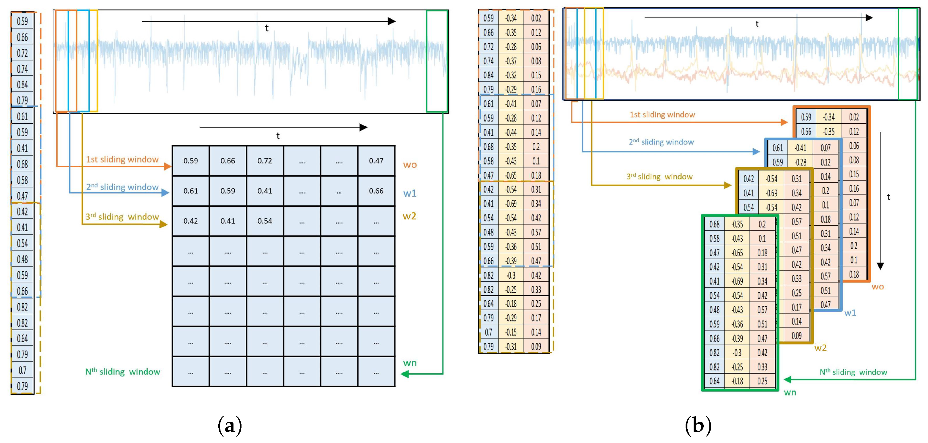
5.2.2. Sliding Window Approach

A sliding window approach was used to segment continuous time-series data into a set of short segments. It is an appropriate way to deal with temporal data because it sequentially processes the raw data keeping into account its temporal behavior. Using this approach divides the data stream into blocks, and it is considered to be a fast segmentation method where no false dismissal can happen because of the overlapping between windows. The sliding window technique convolves along the time axis based on two parameters (i.e., window size W and stride S, which is the step size of sliding a window). Here, the window size W is a determined sampling rate. A fixed sliding window of 30 is adopted in our experiments, and stride S is set to 15. Figure 6a,b present the sliding window approaches that were used in our experiment. The sliding window approach is applied to two different categories of time-series data: univariate time-series data (Figure 6a) and multivariate time-series data (Figure 6b).

5.3. Experiment and Discussion

5.3.1. Experiments Setup

The proposed method was implemented using MatConvNet [177] in Matlab. As a result of the complexity and variability characteristics of the ICBD dataset, obtaining reliable training data normally requires collecting multiple annotations from different experts and then performing cross-validation on the collected labelings. We performed 5-fold cross-validation on the provided classes, splitting them into 5 equal subsets. In each evaluation round, each model was trained on 4 folds and tested on the 5th one. This procedure was repeated for all 5 folds. Both sliding window approaches were applied to extract subsequences from the folds. Moreover, the VeDBA method was applied to the raw tri-axial accelerometer data using Equation (4) to obtain univariate time-series data. Following this, the univariate time-series data was segmented to be used as input data for the k-means and the DAE framework, while the multivariate time-series data was segmented to be used as input data for the DCAE.

The model was trained end-to-end in an unsupervised manner, with no pre-training or fine-tuning procedures involved. All weights were initialized using the Xavier method [178], biases were set to 0, and the cluster centers were initialized randomly. Stochastic gradient descent with mini-batch was used, where each batch contained 32 random shuffled instances. Furthermore, an initial learning rate of 0.006 with a momentum of 0.9 and weight decay of 0.0005 was used. We set $\lambda$, the clustering weight-parameter that controls the loss contribution percentage of clustering error, to 0.1, and the model converged after 100 epochs.

5.3.2. Experimental Results

Evaluation Metrics

To justify our methods, two evaluation approaches are used to compute the cluster quality: Accuracy (ACC) and Normalized Mutual Information (NMI), which distinguish the clustering results generated by our deep cluster method and the ground truth labels.

• Accuracy (ACC): Clustering accuracy is a widely used measurement to evaluate clustering results. It is computed using obtained clustering results and ground truth labels by using the following form [179,180]:

  $$Accuracy=\frac{{\sum }_{i=1}^n\delta (y_i,map\left(c_i\right))}{n},$$

  (6)

  where n is the number of samples, $y_i$ denotes ground truth labels, $c_i$ is obtained clusters, $\delta (y,c)$ is a function that equals one if $y=c$ and zero otherwise, and $map\left(c_i\right)$ is the permutation function that maps obtained cluster labels into their corresponding ground truth labels.
• Normalized Mutual Information (NMI): The NMI is another metric used to measure clustering quality. It is defined between two random variables as [181]:

  $$NMI(X;Y)=\frac{I(X;Y)}{\sqrt{H\left(X\right)H\left(Y\right)}},$$

  (7)

  where X denotes ground truth labels, Y is the obtained cluster, $I(X;Y)$ is the mutual information between X and Y, and $H\left(X\right)$ and $H\left(Y\right)$ denote the utilized entropy, which normalize the value of mutual information into [0, 1] range.

Baseline Methods, Results and Analysis

We compared three different methods: k-means, DAE with embedded clustering, and DCAE with embedded clustering. The results are promising, showing the latent space encodes sufficient patterns to facilitate accurate clustering of animal behaviors through movement.

Table 2. Experimental results of clustering quality, reporting averaged performance across 5-fold cross-validation on three methods on the ICBD.

	ACC	MNI
k-means	37.44	19.73
DAE with embedded clustering	78.67	53.63
DCAE with embedded clustering	94.36	79.40

demonstrates that DCAE with embedded clustering outperforms the other methods, where 79.40% and 94.36% were achieved on NMI and ACC, respectively. It also shows the performance of the clustering algorithm in different spaces, i.e., the original data space and the hidden space learned via non-linear mapping with both DAE and DCAE. The experimental results of the traditional k-means support our hypothesis that conventional clustering algorithms attain limited performance as dimensionality increases. Within the latent space of AE, the clustering algorithm benefits from the DAE, which allows it to deal with learned features rather than raw data. With regard to local temporal information via DCAE, the local salience of the signal shows its ability and allows the clustering algorithm to perform much better. DCAE allows local capture of the salience of signals and the obtaining of the specific variance of signals at different scales, which helps the clustering algorithm deal with the more clustering-friendly representation. It also shows that univariate representation of data in K-means and DAE lost information compared with the multivariate analysis in DCAE.

6. State-of-the-Art and Outlook

Since we applied our deep cluster method to time-series data, deep learning-based clustering methods have become a novel trend and are increasingly adopted in time-series applications with various designs of deep network architectures and clustering methods from several application domains. We review these works, identifying state-of-the-art, and present an outlook on this important field of deep time-series clustering (DTSC) from five important perspectives.

Table 3. Deep Time-series Clustering Methods. RL indicates reconstruction loss.

Categories	DTSC Methods	Year	Architecture	Loss	Clustering Methods	Data Type & Applications
Multi-step	DAN-ECG [182]	2018	DAE	RL	Hierarchical	ECG
	RLPC-DCAE [192]	2018	DCAE	RL	k-means	Load Forecasting
	DEC-ECG [187]	2019	DCAE	RL	GMM	ECG
	CSS-DCAE [191]	2019	DCAE	RL	k-means	Seismology
	STTP-DC [202]	2019	CNN	Multi	k-means	Traffic Analysis
	AE-TSC [190]	2020	DCAE	RL	Kmedoids	Energy (Demand Response)
	CA-MTD [193]	2020	DCAE	RL	k-means	Urban Detection
	TCN-SDF [189]	2020	1D-DCAE	RL	k-means	Operating Machinery
	DM-TSEC [195]	2020	RNN-AE	RL	k-means	ECG
	IBS-DC [198]	2020	RNN-AE	RL	k-means	Animal Motion
	DPC-DP [197]	2020	RNN-AE	Multi	k-means	Disease Progression
Joint	DTC [186]	2018	1D-DCAE	RL	k-means	UCR Archive datasets
	DL-CMCPT [184]	2019	DAE	RL	GMM	Disease Progression
	C-RBE [183]	2019	DAE	RL	k-means	Energy (Demand Response)
	STC-TD [185]	2019	DAE	RL	k-means	Traffic Analysis
	IDTC [188]	2019	DCAE	RL	k-means	Automotive Diagnostic
	DETECT [196]	2019	RNN-AE	RL	k-means	Mobility Analysis
	LR-TSC [200]	2019	S2S-AE	RL	k-means	ECG
	TC-TCM [201]	2020	RNN-AE, DCAE	RL	k-means	Thermal Condition Monitoring
	DC-HA [199]	2020	RNN-AE	RL	k-means	Human Activities

presents a classification of the surveyed papers according to the five perspectives. We believe that the following aspects of DTSC are worthy of further investigation, and could open up promising research directions.

6.1. Different Network Architectures

Since 2018, DTSC has received particular attention with regards to different kinds of network achitecture, such as deep auto-encoder (DAE) [182,183,184,185], deep convolutional auto-encoder (DCAE) [186,187,188,189,190,191,192,193,194], and recurrent neural networks (RNNs), including RNN auto-encoder (RNN-AE) [195,196,197,198] or seq2seq auto-encoder (S2S-AE) [199,200,201]. DTSC can be considered to fall into two pipelines (see Figure 7): the sequential multi-step approach or joint approach. The sequential multi-step approach consists of two main steps (see Figure 7a); the first step learns efficient representations of the time-series data through deep networks, while the second step performs clustering on the learned representations. In the joint approach, learning time-series representation and the clustering process are integrated into a single network model, allowing the extraction of latent features and cluster assignments simultaneously (see Figure 7b).

Two significant steps separate the clustering task from representation learning and feature extraction. Thinsungnoen et al. [182] apply a DAE to learn efficient time-series representatives, demonstrating that time-series data of ECG signals reveals useful hidden information. The learned ECG representations are then fed to an agglomerative hierarchical approach for the clustering process. In the same manner, a DCAE was used to extract latent features of time-series under the influence of temporal distortion [191], demonstrating that the learned latent space is suitable for k-means clustering. The DCAE was also utilized by [192] to map the data of the yearly load profile into a low-dimensionality representative vector. A k-means clustering algorithm was then carried out based on the learned vectors. In [187], ECG records also benefit from deep clustering, where a GMM clustering metric is optimized in the lower-dimensional latent space of DCAE. These techniques are applied to time segments of continuous wavelet transforms of ECG signal, representing a diversity of health conditions. A 1D-convolutional layer’s architecture was also adopted for a deep clustering method [189] to cluster the operating conditions of a system and identify the fault signals not associated with the new conditions clusters. In addition, Guillaume et al. [190] propose 1D-DCAE to learn the features of time-series data, which are used as input to a K-medoids algorithm to perform clustering.

Deep neural networks with embedded clustering have been developed, which simultaneously allow extracting features and clustering assignments within the training process. Inspired by deep image clustering [155], Sai et al. [186] propose deep temporal clustering (DTC), which uses DAE as an initialization method to learn feature representations and indirectly perform clustering. The clustering layer is designed to optimize a Kullback Leibler (KL) divergence objective to enforce a self-training target distribution. The encoding procedure can control the clustering performance, since the predicted distribution is estimated based on the learned representations, which are later fed to k-means for clustering. The concept of deep clustering for static image datasets was also transferred to multivariate time-series data by [188], where 1D-DCAE was utilized to help latent space clustering. High-dimensional time-series data poses some difficulties when looking to effectively model traffic patterns; thus, deep clustering has been employed to jointly perform representation learning and clustering of a large unlabeled dataset [202]. Sun et al. [183] adopted a deep embedded clustering to jointly extract new features and form the clusters for household load in demand response application. Moreover, Lee and Schaar [197] have introduced a deep learning approach for clustering time-series data using a method which consists of several networks: an encoder, a selector, a predictor, and an embedding dictionary. Together, these components provide the cluster assignment and the corresponding centroid based on a given sequence of observations through optimizing joint loss functions. This encourages each cluster to have homogeneous future outcomes (e.g., adverse events, the onset of comorbidities, etc.).

Recurrent Neural Network (RNN) [203,204] and Long Short-Term Memory (LSTM) [205] are the most commonly used techniques for time-series analysis tasks, particularly in supervised learning. However, RNN has recently been exploited for unsupervised clustering. Ienco et al. [195] propose a multivariate time-series clustering method utilizing RNN in a method that employs a Gated Recurrent Unit [206] to encode time-series data into a new vector embedding representation, based on which a centroid-based clustering algorithm (i.e., k-means) is applied on the new data representation. Like the mechanism of a traditional auto-encoder, the RNN encoder maps inputs into a new representation space. The data is projected into a set of feature spaces, using the encoding part, from which a recurrent decoder reconstructs the original data. Yue et al. [196] adopted an RNN auto-encoder to jointly learn embedding latent space behaviors. A clustering-oriented loss is directly built on the embedded features to cluster assignments. The same architecture was adopted by Abedin et al. [199] for human activity recognition. The encoder maps a windowed excerpt of a raw multi-channel sensory sequence into a fixed-length representation as a holistic summary of the input. Once the DAE is pre-trained, a parameterized clustering network is applied as an extension to the framework to refine the latent space and guide the network towards yielding clustering-friendly representations.

The seq2seq [207] is an unsupervised encoder–decoder based model able to learn representations from sequence data, exploiting labels to support the learning process [208]. Two RNNs work together with a unique token, attempting to predict the next state sequence from the previous one. The seq2seq is used by Kiros et al. [209] to learn the sentence representations and predict the context sentences of a given sentence. Gan et al. [210] also used the seq2seq model to predict multiple future sentences. Their experiments demonstrated the benefits of a task-related representation, where model performance can be significantly improved by fine-tuning with a downstream classification task. Motivated by this, Ma et al. [200] proposed deep temporal clustering representation (DTCR), where the learned representations facilitate the clustering task. The original time-series data is mapped through an encoder procedure into latent space representations, which are used to reconstruct the original shape with a decoder part. At the same time, a k-means objective is embedded into the model, allowing latent features and clustering assignments to be learned simultaneously.

Section 5 focused on DAE and DCAE and proposed a deep time-series clustering (DTSC). We were inspired by the results of our proposed method of a deep convolutional auto-encoder with embedded clustering applied to image datasets. Following a similar line of thinking, researchers can further adapt the neural architecture advances in deep clustering in the field of computer vision to satisfy time-series data. However, we argue that there is no ultimate architecture to DTSC, thus, it is a strong starting point to study how various architectures could solve a particular DTSC problem.

Most of the previously described methods rely on the capabilities of the encoder, so the focus is on the auto-encoder architectures. Deep clustering with generative adversarial networks (GANs) [211] for time-series data is a research direction of interest. To the best of our knowledge, time-series clustering tasks have not exploited the full power of GANs, even though they have received attention in the field of computer vision and image processing. For example, GAN has been adopted for clustering by Mukherjee et al. [212], who proposed ClusterGAN, a GAN-based image clustering method. They recovered latent features of image data, exploiting the unconditional GAN to effectively achieve unsupervised clustering in the latent space. The latent variables from a mixture of encoded variables (i.e., one-hot encoded vectors) are jointly trained with clustering-specific loss. Although ClusterGAN has achieved state-of-the-art in the computer vision community, it is currently under-represented in DTSC works. Furthermore, the original GAN was extended to model realistic time-series data [213], demonstrating that time-series GAN (TSGAN) can be a better generator and produce high fidelity and diverse synthetic time-series with low to limited training data. Benefiting from TSGAN, the utilization of ClusterGAN could be applied to the DTSC; this could result in promising future work. Additionally, by integrating the advantages of dense connectivity on the auto-encoder architectures [214], it becomes possible to extract more efficient features and can improve the DTSC efficiency while ensuring high accuracy.

6.2. Different Clustering Methods

Examining the clustering methods utilized in DTSC, the papers surveyed indicate that the trend is dominated by k-means as a commonly applied partitioning method of clustering [183,185,186,188,189,191,192,193,195,196,197,198,199,200,201,202]. The reason for this may be due to its speed, simplicity and ease of implementation. In [188], soft-dynamic time warping (SDTW) [215] was used as an alternative similarity measure to k-means, allowing for the management of dissimilarity evaluation of two time-series of variable length. The SDTW is a smooth formulation of DTW recently introduced to overcome the computational costs of DTW [216]. Other partitioning clustering methods can be efficiently applied to DTSC, such as Richard et al. [190] using a K-medoids algorithm to cluster time-series data on the latent space due to its simplicity and robustness to outliers.

Although popular conventional clustering methods (i.e., hierarchical, model-based, and density-based clustering) have achieved efficient clustering results, they have rarely been used as clustering methods in DTSC frameworks. Driven by the achievements of these conventional methods, exploring the usefulness of adopting them in DTSC is a suggested path. This would open another interesting direction for researchers, as the powerful non-linear transformation would benefit these methods’ performance. For instance, self-organizing maps (SOM) [143] have rarely been used as a clustering algorithm for DTSC. Embedding SOM into the latent space would allow modeling of the latent space and joint learning of the latent representations and code vectors of SOM.

6.3. Deep Learning Heuristics

As one of the concrete examples, data augmentation can help a model learn features that are invariant to transformation and can support learning using the transform invariant approach to facilitate the job of DTSC in producing a significant performance. We believe there is considerable research potential in developing specific augmentation techniques for time-series data, where the temporal aspect of the data can be considered. For instance, Weber et al.’s learnable warping functions [217] can be leveraged so the network can learn the optimal warping features by adopting continuous affine and more complex transformations, which can improve the performance of DTSC.

The use of time-series clustering is due to the lack of labels in such data. Supervision knowledge dramatically assists the formation of discriminative transformations learned by the encoding part of the DCAE, ameliorating the clustering algorithms in the latent space [158]. Even weak or partial supervision knowledge could significantly improve the quality of DTSC. Since semi-supervised learning has allowed us to leverage a large number of unlabeled images efficiently, we assume that DTSC researchers would benefit from adopting this type of procedure to more efficiently guide a large amount of unlabeled time-series data toward obtaining more discriminative data partitioning.

6.4. DTSC Applications

Concerning our classification of time-series data in Section 3, DTSC is applied to different time-series data types from various applications. Multivariate time-series data including disease progression [184,197], ECG signals [182,187,195], demand response [183,190], load forecasting [192], pattern changes in temperature [201], and seismic signal [191] made use of DCAE. Moreover, DTSC provided a great benefit to tensor fields’ data type, including machines (e.g., engines), which typically consist of a large number of sensors or nodes that produce vast amounts of data collected over a period of time [188,189]. In time-series of spatial positions of moving objects, trajectory data presents different places over time, providing a clear idea of spatio-temporal changes. The DTSC method is applied to cluster this type of application to understand and recognize the mobility of a range of moving objects, such as vehicles [185,202] and spacecraft [186], which can lead to path discovery, movement analysis, and location prediction. Discovering behavioral patterns and finding interesting events in certain municipalities’ sectors is considered spatial configurations and distributions. This type of application (i.e., personal mobility behaviors [199] and movement patterns [193,196], and behaviors of animals [198]) has also benefited from DTSC. Time-series data pose challenges for real-world applications because of the data acquisition method and the inherent nature of such data [151]. Based on the aforementioned architectures, methods, and applications, we believe that it would be possible to enable more application domains to access the significant gains of DTSC. For instance, a wide range of applications in action recognition [218] and deep network compression [219,220,221] can benefit from DTSC. Thus, it would be of considerable interest to explore how such applications can make use of DTSC and how its abilities can be improved.

6.5. DTSC Benchmarks

DTSC has been applied to various applications, and we believe it will have an influence on even more application domains in the future, in the same manner as conventional clustering algorithms. The UCR time-series archive [222] has become the state-of-the-art repository of time-series data and an essential resource for the time-series data mining community. The limitation associated with testing time-series clustering algorithms is studied by [223], utilizing all time-series datasets available in the UCR archive for popular conventional clustering methods (i.e., partitional, hierarchical, and density-based, discussed in Section 4.2). Beyond presenting new review papers, especially for DTSC, we believe the generalization of this time-series clustering benchmark to include DTSC methods warrants further study. This can present a useful reference for the research community, and dataset-level assessment metrics can be used to validate the newly proposed methods.

7. Conclusions

As has been shown, deep clustering of time-series data comes with several challenges under continual study. This paper has explicitly examined automatic methods, with a focus on time-series data and machine learning clustering techniques as part of deep time-series clustering (DTSC). A comprehensive review of time-series data analysis was provided, focusing on time-series data and several choices of similarity measures and feature extraction, which significantly influence the quality of analysis techniques. Time-series clustering faces obstacles and difficulties, such as feature representations at different time scales, and the potential for distortion by high-frequency perturbations, random noise in time-series data, and increasing dimensionality. These challenges can make the detection of interesting patterns very difficult for traditional clustering algorithms, but this can be overcome by the adoption of deep learning. We explored the topic of DTSC for the first time and presented a case study. We applied what we proposed in [2] to real-world time-series data in the form of the Imperial Cormorant bird dataset (ICBD) from the Biosciences department at Swansea University. The results were promising, showing that the latent space encodes sufficient patterns to facilitate accurate clustering of movement behaviors. Our study has compared DCAE and DCE, and shown that the clustering performance is efficiently improve by replacing fully-connected layers with convolutional ones. The clustering algorithm also performs much better compared to the original space clustering. We subsequently reviewed other recent state-of-the-art methods, discussed the challenges of DTSC, suggested opportunities and potential future directions for research, and presented an outlook of the field of DTSC from five important perspectives. Finally, as deep learning has attained extraordinary achievements in numerous machine learning fields, especially in computer vision, text mining, speech recognition, and image segmentation, we believe that there is ample scope for DTSC researchers’ exploration, as deep learning models have advanced extremely quickly. We hope this paper can act as a keystone for future research on DTSC.

References

1. Aigner, W.; Miksch, S.; Schumann, H.; Tominski, C. Visualization of Time-Oriented Data; Springer Publishing Company: Berlin/Heidelberg, Germany, 2011. [Google Scholar]
2. Alqahtani, A.; Xie, X.; Deng, J.; Jones, M. A Deep Convolutional Auto-Encoder with Embedded Clustering. In Proceedings of the IEEE International Conference on Image Processing, Athens, Greece, 7–10 October 2018; pp. 4058–4062. [Google Scholar]
3. Hotz, I.; Peikert, R. Definition of a Multifield. In Scientific Visualization: Uncertainty, Multifield, Biomedical, and Scalable Visualization; Hansen, C.D., Chen, M., Johnson, C.R., Kaufman, A.E., Hagen, H., Eds.; Springer: London, UK, 2014; pp. 105–109. [Google Scholar]
4. Zheng, Y.; Liu, Q.; Chen, E.; Ge, Y.; Zhao, J.L. Time series classification using multi-channels deep convolutional neural networks. In Proceedings of the International Conference on Web-Age Information Management, Macau, China, 16–18 June 2014; pp. 298–310. [Google Scholar]
5. Lughofer, E.; Sayed-Mouchaweh, M. Predictive Maintenance in Dynamic Systems: Advanced Methods, Decision Support Tools and Real-World Applications; Springer: Berlin/Heidelberg, Germany, 2019. [Google Scholar]
6. Lughofer, E.; Zavoianu, A.C.; Pollak, R.; Pratama, M.; Meyer-Heye, P.; Zörrer, H.; Eitzinger, C.; Radauer, T. Autonomous supervision and optimization of product quality in a multi-stage manufacturing process based on self-adaptive prediction models. J. Process Control 2019, 76, 27–45. [Google Scholar] [CrossRef]
7. Battke, F.; Symons, S.; Nieselt, K. Mayday-integrative analytics for expression data. BMC Bioinform. 2010, 11, 121. [Google Scholar] [CrossRef] [Green Version]
8. Jeong, D.H.; Darvish, A.; Najarian, K.; Yang, J.; Ribarsky, W. Interactive visual analysis of time-series microarray data. Vis. Comput. 2008, 24, 1053–1066. [Google Scholar] [CrossRef]
9. Vogogias, A.; Kennedy, J.; Archambault, D. Hierarchical Clustering with Multiple-Height Branch-Cut Applied to Short Time-Series Gene Expression Data. In Proceedings of the EuroVis Posters, Groningen, The Netherlands, 6–10 June 2016. [Google Scholar]
10. Cho, M.; Kim, B.; Bae, H.J.; Seo, J. Stroscope: Multi-scale visualization of irregularly measured time-series data. IEEE Trans. Vis. Comput. Graph. 2014, 20, 808–821. [Google Scholar] [CrossRef] [PubMed]
11. Chang, R.; Ghoniem, M.; Kosara, R.; Ribarsky, W.; Yang, J.; Suma, E.; Ziemkiewicz, C.; Kern, D.; Sudjianto, A. Wirevis: Visualization of categorical, time-varying data from financial transactions. In Proceedings of the IEEE Symposium on Visual Analytics Science and Technology, Sacramento, CA, USA, 30 October–1 November 2007; pp. 155–162. [Google Scholar]
12. Xie, C.; Chen, W.; Huang, X.; Hu, Y.; Barlowe, S.; Yang, J. VAET: A visual analytics approach for e-transactions time-series. IEEE Trans. Vis. Comput. Graph. 2014, 20, 1743–1752. [Google Scholar] [CrossRef] [Green Version]
13. Turkay, C.; Kaya, E.; Balcisoy, S.; Hauser, H. Designing progressive and interactive analytics processes for high-dimensional data analysis. IEEE Trans. Vis. Comput. Graph. 2017, 23, 131–140. [Google Scholar] [CrossRef]
14. Lei, S.T.; Zhang, K. A visual analytics system for financial time-series data. In Proceedings of the International Symposium on Visual Information Communication, Beijing, China, 28–29 September 2010; pp. 1–9. [Google Scholar]
15. Ziegler, H.; Jenny, M.; Gruse, T.; Keim, D.A. Visual market sector analysis for financial time series data. In Proceedings of the IEEE Symposium on Visual Analytics Science and Technology, Salt Lake City, UT, USA, 24–29 October 2010; pp. 83–90. [Google Scholar]
16. Schreck, T.; Bernard, J.; Von Landesberger, T.; Kohlhammer, J. Visual cluster analysis of trajectory data with interactive kohonen maps. Inf. Vis. 2009, 8, 14–29. [Google Scholar] [CrossRef] [Green Version]
17. Schreck, T.; Tekušová, T.; Kohlhammer, J.; Fellner, D. Trajectory-based visual analysis of large financial time series data. ACM SIGKDD Explor. Newsl. 2007, 9, 30–37. [Google Scholar] [CrossRef] [Green Version]
18. Perer, A.; Sun, J. MatrixFlow: Temporal network visual analytics to track symptom evolution during disease progression. In Proceedings of the AMIA Annual Symposium, Chicago, IL, USA, 3–7 November 2012; Volume 2012, pp. 716–725. [Google Scholar]
19. Guo, S.; Xu, K.; Zhao, R.; Gotz, D.; Zha, H.; Cao, N. EventThread: Visual Summarization and Stage Analysis of Event Sequence Data. IEEE Trans. Vis. Comput. Graph. 2018, 24, 56–65. [Google Scholar] [CrossRef]
20. Wang, Y.; Wu, T.; Chen, Z.; Luo, Q.; Qu, H. Stac: Enhancing stacked graphs for time series analysis. In Proceedings of the IEEE Pacific Visualization Symposium, Taipei, Taiwan, 19–22 April 2016; pp. 234–238. [Google Scholar]
21. Wilkinson, L. Visualizing Big Data Outliers through Distributed Aggregation. IEEE Trans. Vis. Comput. Graph. 2017, 24, 256–266. [Google Scholar] [CrossRef] [PubMed]
22. Meidiana, A.; Hong, S.H. MultiStory: Visual analytics of dynamic multi-relational networks. In Proceedings of the IEEE Pacific Visualization Symposium, Hangzhou, China, 14–17 April 2015; pp. 75–79. [Google Scholar]
23. Goodfellow, I.; Bengio, Y.; Courville, A. Deep Learning; MIT Press: Cambridge, MA, USA, 2016. [Google Scholar]
24. Hadlak, S.; Schumann, H.; Cap, C.H.; Wollenberg, T. Supporting the visual analysis of dynamic networks by clustering associated temporal attributes. IEEE Trans. Vis. Comput. Graph. 2013, 19, 2267–2276. [Google Scholar] [CrossRef] [PubMed]
25. Steiger, M.; Bernard, J.; Mittelstadt, S.; Lucke-Tieke, H.; Keim, D.; May, T.; Kohlhammer, J. Visual Analysis of Time-Series Similarities for Anomaly Detection in Sensor Networks. Comput. Graph. Forum 2014, 33, 401–410. [Google Scholar] [CrossRef]
26. van den Elzen, S.; Holten, D.; Blaas, J.; van Wijk, J.J. Reducing snapshots to points: A visual analytics approach to dynamic network exploration. IEEE Trans. Vis. Comput. Graph. 2016, 22, 1–10. [Google Scholar] [CrossRef] [PubMed]
27. Zhou, F.; Huang, W.; Zhao, Y.; Shi, Y.; Liang, X.; Fan, X. Entvis: A visual analytic tool for entropy-based network traffic anomaly detection. IEEE Comput. Graph. Appl. 2015, 35, 42–50. [Google Scholar] [CrossRef]
28. Fujiwara, T.; Li, J.K.; Mubarak, M.; Ross, C.; Carothers, C.D.; Ross, R.B.; Ma, K.L. A visual analytics system for optimizing the performance of large-scale networks in supercomputing systems. Vis. Inform. 2018, 2, 98–110. [Google Scholar] [CrossRef]
29. Cao, N.; Shi, C.; Lin, S.; Lu, J.; Lin, Y.R.; Lin, C.Y. TargetVue: Visual analysis of anomalous user behaviors in online communication systems. IEEE Trans. Vis. Comput. Graph. 2016, 22, 280–289. [Google Scholar] [CrossRef]
30. Hao, M.C.; Marwah, M.; Janetzko, H.; Keim, D.i.A.; Dayal, U.; Sharma, R.; Patnaik, D.; Ramakrish-nan, N. Visual analysis of frequent patterns in large time series. In Proceedings of the IEEE Symposium on Visual Analytics Science and Technology, Salt Lake City, UT, USA, 24–29 October 2010; pp. 227–228. [Google Scholar]
31. Muelder, C.; Zhu, B.; Chen, W.; Zhang, H.; Ma, K.L. Visual analysis of cloud computing performance using behavioral lines. IEEE Trans. Vis. Comput. Graph. 2016, 22, 1694–1704. [Google Scholar] [CrossRef] [PubMed]
32. Sharma, G.; Shroff, G.; Pandey, A.; Singh, B.; Sehgal, G.; Paneri, K.; Agarwal, P. Multi-sensor visual analytics supported by machine-learning models. In Proceedings of the International Conference on Data Mining Workshop, Atlantic City, NJ, USA, 14–17 November 2015; pp. 668–674. [Google Scholar]
33. Shi, L.; Liao, Q.; He, Y.; Li, R.; Striegel, A.; Su, Z. SAVE: Sensor anomaly visualization engine. In Proceedings of the IEEE Conference on Visual Analytics Science and Technology, Providence, RI, USA, 23–28 October 2011; pp. 201–210. [Google Scholar]
34. Arbesser, C.; Spechtenhauser, F.; Mühlbacher, T.; Piringer, H. Visplause: Visual data quality assessment of many time series using plausibility checks. IEEE Trans. Vis. Comput. Graph. 2017, 23, 641–650. [Google Scholar] [CrossRef]
35. Chen, Y.; Xu, P.; Ren, L. Sequence Synopsis: Optimize Visual Summary of Temporal Event Data. IEEE Trans. Vis. Comput. Graph. 2018, 24, 45–55. [Google Scholar] [CrossRef]
36. Andrienko, G.; Andrienko, N.; Wrobel, S. Visual analytics tools for analysis of movement data. ACM SIGKDD Explor. Newsl. 2007, 9, 38–46. [Google Scholar] [CrossRef]
37. Andrienko, G.; Andrienko, N. Spatio-temporal aggregation for visual analysis of movements. In Proceedings of the IEEE Symposium on Visual Analytics Science and Technology, Columbus, OH, USA, 19–24 October 2008; pp. 51–58. [Google Scholar]
38. Andrienko, G.; Andrienko, N.; Hurter, C.; Rinzivillo, S.; Wrobel, S. From movement tracks through events to places: Extracting and characterizing significant places from mobility data. In Proceedings of the IEEE Conference on Visual Analytics Science and Technology, Providence, RI, USA, 23–28 October 2011; pp. 161–170. [Google Scholar]
39. Andrienko, G.; Andrienko, N.; Hurter, C.; Rinzivillo, S.; Wrobel, S. Scalable Analysis of Movement Data for Extracting and Exploring Significant Places. IEEE Trans. Vis. Comput. Graph. 2013, 19, 1078–1094. [Google Scholar] [CrossRef] [PubMed] [Green Version]
40. Lu, M.; Wang, Z.; Yuan, X. Trajrank: Exploring travel behaviour on a route by trajectory ranking. In Proceedings of the IEEE Pacific Visualization Symposium, Hangzhou, China, 14–17 April 2015; pp. 311–318. [Google Scholar]
41. Andrienko, G.; Andrienko, N.; Rinzivillo, S.; Nanni, M.; Pedreschi, D.; Giannotti, F. Interactive visual clustering of large collections of trajectories. In Proceedings of the IEEE Symposium on Visual Analytics Science and Technology, Atlantic City, NJ, USA, 11–16 October 2009; pp. 3–10. [Google Scholar]
42. Riveiro, M.; Lebram, M.; Elmer, M. Anomaly detection for road traffic: A visual analytics framework. IEEE Trans. Intell. Transp. Syst. 2017, 18, 2260–2270. [Google Scholar] [CrossRef]
43. Kalamaras, I.; Zamichos, A.; Salamanis, A.; Drosou, A.; Kehagias, D.D.; Margaritis, G.; Papadopoulos, S.; Tzovaras, D. An interactive visual analytics platform for smart intelligent transportation systems management. IEEE Trans. Intell. Transp. Syst. 2018, 19, 487–496. [Google Scholar] [CrossRef]
44. Andrienko, G.; Andrienko, N.; Mladenov, M.; Mock, M.; Pölitz, C. Identifying place histories from activity traces with an eye to parameter impact. IEEE Trans. Vis. Comput. Graph. 2012, 18, 675–688. [Google Scholar] [CrossRef] [PubMed] [Green Version]
45. Andrienko, G.L.; Andrienko, N.V.; Fuchs, G.; Raimond, A.M.O.; Symanzik, J.; Ziemlicki, C. Extracting Semantics of Individual Places from Movement Data by Analyzing Temporal Patterns of Visits. In Proceedings of the ACM SIGSPATIAL International Workshop on Computational Models of Place, Orlando, FL, USA, 5 November 2013; pp. 9–15. [Google Scholar]
46. Chae, J.; Wang, G.; Ahlbrand, B.; Gorantla, M.B.; Zhang, J.; Chen, S.; Xu, H.; Zhao, J.; Hatton, W.; Malik, A.; et al. Visual analytics of heterogeneous data for criminal event analysis VAST challenge 2015: Grand challenge. In Proceedings of the IEEE Conference on Visual Analytics Science and Technology, Chicago, IL, USA, 25–30 October 2015; pp. 149–150. [Google Scholar]
47. Pu, J.; Liu, S.; Xu, P.; Qu, H.; Ni, L.M. MViewer: Mobile phone spatiotemporal data viewer. Front. Comput. Sci. 2014, 8, 298–315. [Google Scholar] [CrossRef]
48. Shen, Z.; Ma, K.L. Mobivis: A visualization system for exploring mobile data. In Proceedings of the IEEE Pacific Visualization Symposium, Kyoto, Japan, 5–7 March 2008; pp. 175–182. [Google Scholar]
49. Zhao, J.; Wang, G.; Chae, J.; Xu, H.; Chen, S.; Hatton, W.; Towers, S.; Gorantla, M.B.; Ahlbrand, B.; Zhang, J.; et al. ParkAnalyzer: Characterizing the movement patterns of visitors VAST 2015 Mini-Challenge 1. In Proceedings of the IEEE Conference on Visual Analytics Science and Technology, Chicago, IL, USA, 25–30 October 2015; pp. 179–180. [Google Scholar]
50. von Landesberger, T.; Brodkorb, F.; Roskosch, P.; Andrienko, N.; Andrienko, G.; Kerren, A. Mobilitygraphs: Visual analysis of mass mobility dynamics via spatio-temporal graphs and clustering. IEEE Trans. Vis. Comput. Graph. 2016, 22, 11–20. [Google Scholar] [CrossRef] [PubMed] [Green Version]
51. Biswas, A.; Lin, G.; Liu, X.; Shen, H.W. Visualization of time-varying weather ensembles across multiple resolutions. IEEE Trans. Vis. Comput. Graph. 2017, 23, 841–850. [Google Scholar] [CrossRef] [PubMed]
52. Senaratne, H.; Mueller, M.; Behrisch, M.; Lalanne, F.; Bustos-Jiménez, J.; Schneidewind, J.; Keim, D.; Schreck, T. Urban Mobility Analysis With Mobile Network Data: A Visual Analytics Approach. IEEE Trans. Intell. Transp. Syst. 2018, 19, 1537–1546. [Google Scholar] [CrossRef] [Green Version]
53. Stopar, L.; Skraba, P.; Grobelnik, M.; Mladenic, D. StreamStory: Exploring Multivariate Time Series on Multiple Scales. IEEE Trans. Vis. Comput. Graph. 2018, 25, 1788–1802. [Google Scholar] [CrossRef]
54. Gao, L.; Campbell, H.A.; Bidder, O.R.; Hunter, J. A Web-based semantic tagging and activity recognition system for species’ accelerometry data. Ecol. Inform. 2013, 13, 47–56. [Google Scholar] [CrossRef]
55. Walker, J.S.; Jones, M.W.; Laramee, R.S.; Bidder, O.R.; Williams, H.J.; Scott, R.; Shepard, E.L.; Wilson, R.P. TimeClassifier: A visual analytic system for the classification of multi-dimensional time series data. Vis. Comput. 2015, 31, 1067–1078. [Google Scholar] [CrossRef] [Green Version]
56. Bernard, J.; Wilhelm, N.; Scherer, M.; May, T.; Schreck, T. TimeSeriesPaths: Projection-based explorative analysis of multivariate time series data. J. WSCG 2012, 2, 97–106. [Google Scholar]
57. Kincaid, R.; Lam, H. Line graph explorer: Scalable display of line graphs using focus+ context. In Proceedings of the Conference on Advanced Visual Interfaces, Venezia, Italy, 23–26 May 2006; pp. 404–411. [Google Scholar]
58. Li, J.; Xiao, Z.; Zhao, H.Q.; Meng, Z.P.; Zhang, K. Visual analytics of smogs in China. J. Vis. 2016, 19, 461–474. [Google Scholar] [CrossRef]
59. Li, J.; Zhang, K.; Meng, Z.P. Vismate: Interactive visual analysis of station-based observation data on climate changes. In Proceedings of the Conference Visual Analytics Science and Technology, Paris, France, 25–31 October 2014; pp. 133–142. [Google Scholar]
60. Martin, S.; Quach, T.T. Interactive visualization of multivariate time series data. In Proceedings of the International Conference on Augmented Cognition, Toronto, ON, Canada, 17–22 July 2016; pp. 322–332. [Google Scholar]
61. Shu, Q.; Guo, H.; Liang, J.; Che, L.; Liu, J.; Yuan, X. EnsembleGraph: Interactive visual analysis of spatiotemporal behaviors in ensemble simulation data. In Proceedings of the IEEE Pacific Visualization Symposium, Taipei, Taiwan, 19–22 April 2016; pp. 56–63. [Google Scholar]
62. Wu, W.; Zheng, Y.; Qu, H.; Chen, W.; Gröller, E.; Ni, L.M. Boundaryseer: Visual analysis of 2d boundary changes. In Proceedings of the IEEE Conference on Visual Analytics Science and Technology, Paris, France, 25–31 October 2014; pp. 143–152. [Google Scholar]
63. Bernard, J.; Wilhelm, N.; Krüger, B.; May, T.; Schreck, T.; Kohlhammer, J. Motionexplorer: Exploratory search in human motion capture data based on hierarchical aggregation. IEEE Trans. Vis. Comput. Graph. 2013, 19, 2257–2266. [Google Scholar] [CrossRef] [Green Version]
64. Blascheck, T.; John, M.; Kurzhals, K.; Koch, S.; Ertl, T. Va 2: A visual analytics approach for evaluating visual analytics applications. IEEE Trans. Vis. Comput. Graph. 2016, 22, 61–70. [Google Scholar] [CrossRef]
65. Purwantiningsih, O.; Sallaberry, A.; Andary, S.; Seilles, A.; Aze, J. Visual analysis of body movement in serious games for healthcare. In Proceedings of the IEEE Pacific Visualization Symposium, Taipei, Taiwan, 19–22 April 2016; pp. 229–233. [Google Scholar]
66. Kim, J.G.; Snodgrass, M.; Pietrowicz, M.; Karahalios, K. Visual Analysis of Relationships between Behavioral and Physiological Sensor Data. In Proceedings of the International Conference on Healthcare Informatics, Dallas, TX, USA, 21–23 October 2015; pp. 170–179. [Google Scholar]
67. Turkay, C.; Parulek, J.; Reuter, N.; Hauser, H. Interactive visual analysis of temporal cluster structures. Comput. Graph. Forum 2011, 30, 711–720. [Google Scholar] [CrossRef]
68. Soriano-Vargas, A.; Vani, B.C.; Shimabukuro, M.H.; Monico, J.F.; Oliveira, M.C.F.; Hamann, B. Visual analytics of time-varying multivariate ionospheric scintillation data. Comput. Graph. 2017, 68, 96–107. [Google Scholar] [CrossRef] [Green Version]
69. Trajcevski, G.; Gunopulos, D.; Aggarwal, C.C.; Reddy, C. Time-series data clustering. In Data Clustering: Algorithms and Applications; Chapman and Hall/CRC: Boca Raton, FL, USA, 2013; pp. 357–375. [Google Scholar]
70. Xing, Z.; Pei, J.; Keogh, E. A brief survey on sequence classification. ACM SIGKDD Explor. Newsl. 2010, 12, 40–48. [Google Scholar] [CrossRef]
71. Sorzano, C.O.S.; Vargas, J.; Montano, A.P. A survey of dimensionality reduction techniques. arXiv 2014, arXiv:1403.2877. [Google Scholar]
72. Liao, T.W. Clustering of time series data—A survey. Pattern Recognit. 2005, 38, 1857–1874. [Google Scholar] [CrossRef]
73. Fulcher, B.D.; Jones, N.S. Highly comparative feature-based time-series classification. IEEE Trans. Knowl. Data Eng. 2014, 26, 3026–3037. [Google Scholar] [CrossRef] [Green Version]
74. Aghabozorgi, S.; Shirkhorshidi, A.S.; Wah, T.Y. Time-series clustering—A decade review. Inf. Syst. 2015, 53, 16–38. [Google Scholar] [CrossRef]
75. Tucci, M.; Raugi, M. Analysis of spectral clustering algorithms for linear and nonlinear time series. In Proceedings of the International Conference on Intelligent Systems Design and Applications, Córdoba, Spain, 22–24 November 2011; pp. 925–930. [Google Scholar]
76. Batóg, J.; Batóg, B. Synchronization of Business Cycles in the EU: Time Series Clustering. WSEAS Trans. Bus. Econ. 2019, 16, 298–305. [Google Scholar]
77. Petitjean, F.; Ketterlin, A.; Gançarski, P. A global averaging method for dynamic time warping, with applications to clustering. Pattern Recognit. 2011, 44, 678–693. [Google Scholar] [CrossRef]
78. Yang, J.; Leskovec, J. Patterns of temporal variation in online media. In Proceedings of the ACM International Conference on Web Search and Data Mining, Hong Kong, China, 9–12 February 2011; pp. 177–186. [Google Scholar]
79. Paparrizos, J.; Gravano, L. k-shape: Efficient and accurate clustering of time series. In Proceedings of the ACM SIGMOD International Conference on Management of Data, Melbourne, Australia, 31 May–4 June 2015; pp. 1855–1870. [Google Scholar]
80. Ferreira, L.N.; Zhao, L. Time series clustering via community detection in networks. Inf. Sci. 2016, 326, 227–242. [Google Scholar] [CrossRef] [Green Version]
81. Guo, C.; Jia, H.; Zhang, N. Time series clustering based on ICA for stock data analysis. In Proceedings of the International Conference on Wireless Communications, Networking and Mobile Computing, Avignon, France, 12–14 October 2008; pp. 1–4. [Google Scholar]
82. Zakaria, J.; Mueen, A.; Keogh, E. Clustering time series using unsupervised-shapelets. In Proceedings of the International Conference on Data Mining, Brussels, Belgium, 10–13 December 2012; pp. 785–794. [Google Scholar]
83. Theodor, P. Time Series Analysis for Assessing and Forecasting of Road Traffic Accidents -Case Studies. WSEAS Trans. Math. 2020, 19, 177–185. [Google Scholar]
84. Shi, L.; Du, L.; Shen, Y.D. Robust spectral learning for unsupervised feature selection. In Proceedings of the International Conference on Data Mining, Shenzhen, China, 14–17 December 2014; pp. 977–982. [Google Scholar]
85. Qian, M.; Zhai, C. Robust unsupervised feature selection. In Proceedings of the International Joint Conference on Artificial Intelligence, Beijing, China, 3–9 August 2013; pp. 1621–1627. [Google Scholar]
86. Li, Z.; Yang, Y.; Liu, J.; Zhou, X.; Lu, H. Unsupervised feature selection using nonnegative spectral analysis. In Proceedings of the AAAI Conference on Artificial Intelligence, Toronto, ON, Canada, 22–26 July 2012; pp. 1026–1032. [Google Scholar]
87. Yang, Y.; Shen, H.T.; Ma, Z.; Huang, Z.; Zhou, X. L2,1-norm regularized discriminative feature selection for unsupervised learning. In Proceedings of the International Joint Conference on Artificial Intelligence, Barcelona, Spain, 16–22 July 2011; pp. 1589–1594. [Google Scholar]
88. Ma, Q.; Li, S.; Shen, L.; Wang, J.; Wei, J.; Yu, Z.; Cottrell, G. End-to-End Incomplete Time-Series Modeling From Linear Memory of Latent Variables. IEEE Trans. Cybern. 2020, 50, 4908–4920. [Google Scholar] [CrossRef] [PubMed] [Green Version]
89. Lei, H.; Xia, Y.; Qin, X. Estimation of semivarying coefficient time series models with ARMA errors. Ann. Stat. 2016, 44, 1618–1660. [Google Scholar] [CrossRef]
90. Cai, Z.; Fan, J.; Yao, Q. Functional-Coefficient Regression Models for Nonlinear Time Series. J. Am. Stat. Assoc. 1999, 95, 941–956. [Google Scholar] [CrossRef]
91. Tjostheim, D.; Auestad, B. Nonparametric Identification of Nonlinear Time Series: Projections. J. Am. Stat. Assoc. 1994, 89, 1398–1409. [Google Scholar]
92. Wang, X.; Mueen, A.; Ding, H.; Trajcevski, G.; Scheuermann, P.; Keogh, E. Experimental comparison of representation methods and distance measures for time series data. Data Min. Knowl. Discov. 2013, 26, 275–309. [Google Scholar] [CrossRef] [Green Version]
93. Tornai, K.; Kovács, L.; Oláh, A.; Drenyovszki, R.; Pintér, I.; Tisza, D.; Levendovszky, J. Classification for consumption data in smart grid based on forecasting time series. Electr. Power Syst. Res. 2016, 141, 191–201. [Google Scholar] [CrossRef]
94. Yahyaoui, H.; Al-Mutairi, A. A feature-based trust sequence classification algorithm. Inf. Sci. 2016, 328, 455–484. [Google Scholar] [CrossRef]
95. Wei, L.; Keogh, E. Semi-supervised time series classification. In Proceedings of the International Conference on Knowledge Discovery and Data Mining, Philadelphia, PA, USA, 20–23 August 2006; pp. 748–753. [Google Scholar]
96. Ye, J.; Xiao, C.; Esteves, R.M.; Rong, C. Time Series Similarity Evaluation Based on Spearman’s Correlation Coefficients and Distance Measures. In Proceedings of the International Conference on Cloud Computing and Big Data in Asia, Huangshan, China, 17–19 June 2015; pp. 319–331. [Google Scholar]
97. Buono, P.; Aris, A.; Plaisant, C.; Khella, A.; Shneiderman, B. Interactive pattern search in time series. Electron. Imaging 2005, 5669, 175–186. [Google Scholar]
98. Yu, D.; Yu, X.; Hu, Q.; Liu, J.; Wu, A. Dynamic time warping constraint learning for large margin nearest neighbor classification. Inf. Sci. 2011, 181, 2787–2796. [Google Scholar] [CrossRef]
99. Zhao, J.; Itti, L. shapeDTW: Shape Dynamic Time Warping. Pattern Recognit. 2018, 74, 171–184. [Google Scholar] [CrossRef] [Green Version]
100. Ratanamahatana, C.A.; Keogh, E. Making time-series classification more accurate using learned constraints. In Proceedings of the SIAM International Conference on Data Mining, Lake Buena Vista, FL, USA, 22–24 April 2004; pp. 11–22. [Google Scholar]
101. Mueen, A.; Keogh, E. Extracting Optimal Performance from Dynamic Time Warping. In Proceedings of the International Conference on Knowledge Discovery and Data Mining, San Francisco, CA, USA, 13–17 August 2016; pp. 2129–2130. [Google Scholar]
102. Kotas, M.; Leski, J.M.; Moroń, T. Dynamic time warping based on modified alignment costs for evoked potentials averaging. In Man–Machine Interactions 4; Springer: Cham, Switzerland, 2016; pp. 305–314. [Google Scholar]
103. Faloutsos, C.; Ranganathan, M.; Manolopoulos, Y. Fast Subsequence Matching in Time-Series Databases; ACM: New York, NY, USA, 1994; Volume 23. [Google Scholar]
104. Berndt, D.J.; Clifford, J. Using Dynamic Time Warping to Find Patterns in Time Series. In Proceedings of the Workshop on Knowledge Discovery in Databases, Seattle, WA, USA, July 1994; pp. 359–370. [Google Scholar]
105. Keogh, E.; Ratanamahatana, C.A. Exact indexing of dynamic time warping. Knowl. Inf. Syst. 2005, 7, 358–386. [Google Scholar] [CrossRef]
106. Vlachos, M.; Kollios, G.; Gunopulos, D. Discovering similar multidimensional trajectories. In Proceedings of the International Conference on Data Engineering, San Jose, CA, USA, 26 February–1 March 2002; pp. 673–684. [Google Scholar]
107. Smith, S. Digital Signal Processing: A practical Guide for Engineers and Scientists; Elsevier: Amsterdam, The Netherlands, 2013. [Google Scholar]
108. Kaya, H.; Gündüz-Öğüdücü, Ş. A distance based time series classification framework. Inf. Syst. 2015, 51, 27–42. [Google Scholar] [CrossRef]
109. Yang, K.; Shahabi, C. A PCA-based similarity measure for multivariate time series. In Proceedings of the ACM International Workshop on Multimedia Databases, Washington, DC, USA, 13 November 2004; pp. 65–74. [Google Scholar]
110. Singhal, A.; Seborg, D.E. Clustering multivariate time-series data. J. Chemom. 2005, 19, 427–438. [Google Scholar] [CrossRef]
111. Yang, K.; Shahabi, C. On the stationarity of multivariate time series for correlation-based data analysis. In Proceedings of the International Conference on Data Mining, Houston, TX, USA, 27–30 November 2005; p. 4. [Google Scholar]
112. Lesch, R.H.; Caillé, Y.; Lowe, D. Component analysis in financial time series. In Proceedings of the Conference on Computational Intelligence for Financial Engineering, New York, NY, USA, 27 April 1999; pp. 183–190. [Google Scholar]
113. Lin, T.; Guo, F.; Wu, Y.; Zhu, B.; Zhang, F.; Qu, H.; Chen, W. TieVis: Visual analytics of evolution of interpersonal ties. In Proceedings of the International Conference on Technologies for E-Learning and Digital Entertainment, Hangzhou, China, 14–16 April 2016; pp. 412–424. [Google Scholar]
114. Dong, G.; Pei, J. Sequence Data Mining; Springer: Berlin/Heidelberg, Germany, 2007; Volume 33. [Google Scholar]
115. Fu, T.c. A review on time series data mining. Eng. Appl. Artif. Intell. 2011, 24, 164–181. [Google Scholar] [CrossRef]
116. Agrawal, R.; Faloutsos, C.; Swami, A. Efficient similarity search in sequence databases. In Proceedings of the International Conference on Foundations of Data Organization and Algorithms, Chicago, IL, USA, 13–15 October 1993; pp. 69–84. [Google Scholar]
117. Rafiei, D.; Mendelzon, A.O. Querying time series data based on similarity. IEEE Trans. Knowl. Data Eng. 2000, 12, 675–693. [Google Scholar] [CrossRef]
118. Janacek, G.J.; Bagnall, A.J.; Powell, M. A likelihood ratio distance measure for the similarity between the fourier transform of time series. In Proceedings of the Pacific Asia Conference on Knowledge Discovery and Data Mining, Hanoi, Vietnam, 18–20 May 2005; pp. 737–743. [Google Scholar]
119. Popivanov, I.; Miller, R.J. Similarity search over time-series data using wavelets. In Proceedings of the International Conference on Data Engineering, San Jose, CA, USA, 26 February–1 March 2002; pp. 212–221. [Google Scholar]
120. Chan, K.P.; Fu, A.W.C. Efficient time series matching by wavelets. In Proceedings of the International Conference on Data Engineering, Sydney, Australia, 23–26 March 1999; pp. 126–133. [Google Scholar]
121. Aggarwal, C.C. On effective classification of strings with wavelets. In Proceedings of the International Conference on Knowledge Discovery and Data Mining, Edmonton, AB, Canada, 23–26 July 2002; pp. 163–172. [Google Scholar]
122. Li, D.; Bissyande, T.F.D.A.; Klein, J.; Le Traon, Y. Time Series Classification with Discrete Wavelet Transformed Data: Insights from an Empirical Study. In Proceedings of the International Conference on Software Engineering and Knowledge Engineering, Redwood City, CA, USA, 1–3 July 2016; pp. 1361–1377. [Google Scholar]
123. Ye, L.; Keogh, E. Time series shapelets: A new primitive for data mining. In Proceedings of the International Conference on Knowledge discovery and Data Mining, Paris, France, 28 June–1 July 2009; pp. 947–956. [Google Scholar]
124. Xing, Z.; Pei, J.; Philip, S.Y.; Wang, K. Extracting Interpretable Features for Early Classification on Time Series. In Proceedings of the SIAM International Conference on Data Mining, Mesa, AZ, USA, 28–30 April 2011; Volume 11, pp. 247–258. [Google Scholar]
125. Ali, M.; Alqahtani, A.; Jones, M.W.; Xie, X. Clustering and Classification for Time Series Data in Visual Analytics: A Survey. IEEE Access 2019, 7, 181314–181338. [Google Scholar] [CrossRef]
126. MacQueen, J. Some methods for classification and analysis of multivariate observations. In Proceedings of the Berkeley Symposium on Mathematical Statistics and Probability; University of California Press: Berkeley, CA, USA, 1967; pp. 281–297. [Google Scholar]
127. Kaufman, L.; Rousseeuw, P.J. Finding Groups in Data: An Introduction to Cluster Analysis; John Wiley & Sons: Hoboken, NJ, USA, 2009; Volume 344. [Google Scholar]
128. Dunn, J.C. A Fuzzy Relative of the ISODATA Process and Its Use in Detecting Compact Well-Separated Clusters; Taylor & Francis: Tokyo, Japan, 1973. [Google Scholar]
129. Bezdek, J.C. Pattern Recognition with Fuzzy Objective Function Algorithms; Book Series: Advanced Applications in Pattern Recognition; Springer: New York, NY, USA; Philadelphia, PA, USA, 1981. [Google Scholar]
130. Krishnapuram, R.; Joshi, A.; Nasraoui, O.; Yi, L.y. Low-complexity fuzzy relational clustering algorithms for web mining. IEEE Trans. Fuzzy Syst. 2001, 9, 595–607. [Google Scholar] [CrossRef] [Green Version]
131. Goutte, C.; Toft, P.; Rostrup, E.; Nielsen, F.A.; Hansen, L.K. On clustering fMRI time series. NeuroImage 1999, 9, 298–310. [Google Scholar] [CrossRef] [Green Version]
132. Niennattrakul, V.; Ratanamahatana, C.A. On clustering multimedia time series data using k-means and dynamic time warping. In Proceedings of the International Conference on Multimedia and Ubiquitous Engineering, Seoul, Korea, 26–28 April 2007; pp. 733–738. [Google Scholar]
133. Meesrikamolkul, W.; Niennattrakul, V.; Ratanamahatana, C.A. Shape-based clustering for time series data. In Proceedings of the Pacific Asia Conference on Knowledge Discovery and Data Mining, Kuala Lumpur, Malaysia, 29 May–1 June 2012; pp. 530–541. [Google Scholar]
134. Hautamaki, V.; Nykanen, P.; Franti, P. Time-series clustering by approximate prototypes. In Proceedings of the International Conference on Pattern Recognition, Tampa, FL, USA, 8–11 December 2008; pp. 1–4. [Google Scholar]
135. Kalpakis, K.; Gada, D.; Puttagunta, V. Distance measures for effective clustering of ARIMA time-series. In Proceedings of the International Conference on Data Mining, San Jose, CA, USA, 29 November–2 December 2001; pp. 273–280. [Google Scholar]
136. Möller-Levet, C.S.; Klawonn, F.; Cho, K.H.; Wolkenhauer, O. Fuzzy clustering of short time-series and unevenly distributed sam-pling points. In Proceedings of the International Symposium on Intelligent Data Analysis, Berlin, Germany, 28–30 August 2003; pp. 330–340. [Google Scholar]
137. Golay, X.; Kollias, S.; Stoll, G.; Meier, D.E.; Valavanis, A.; Boesiger, P. A new correlation-based fuzzy logic clustering algorithm for FMRI. Magn. Reson. Med. 1998, 40, 249–260. [Google Scholar] [CrossRef]
138. D’Urso, P.; Cappelli, C.; Lallo, D.D.; Massari, R. Clustering of financial time series. Phys. A Stat. Mech. Its Appl. 2013, 392, 2114–2129. [Google Scholar] [CrossRef]
139. Das, S.; Abraham, A.; Konar, A. Automatic clustering using an improved differential evolution algorithm. IEEE Trans. Syst. Man, Cybern.-Part A Syst. Hum. 2008, 38, 218–237. [Google Scholar] [CrossRef]
140. Van Wijk, J.J.; Van Selow, E.R. Cluster and calendar based visualization of time series data. In Proceedings of the IEEE Symposium on Information Visualization, San Francisco, CA, USA, 24–29 October 1999; pp. 4–9. [Google Scholar]
141. Simonsen, M.; Mailund, T.; Pedersen, C.N.S. Rapid Neighbour-Joining. In Proceedings of the International Workshop on Algorithms in Bioinformatics, Karlsruhe, Germany, 15–19 September 2008; pp. 113–122. [Google Scholar]
142. Alkhushayni, S.; Choi, T.; Alzaleq, D. Data analysis using representation theory and clustering algorithms. WSEAS Trans. Comput. 2020, 19, 310–320. [Google Scholar] [CrossRef]
143. Kohonen, T. The self-organizing map. Proc. IEEE 1990, 78, 1464–1480. [Google Scholar] [CrossRef]
144. Sacha, D.; Kraus, M.; Bernard, J.; Behrisch, M.; Schreck, T.; Asano, Y.; Keim, D.A. Somflow: Guided exploratory cluster analysis with self-organizing maps and analytic provenance. IEEE Trans. Vis. Comput. Graph. 2018, 24, 120–130. [Google Scholar] [CrossRef] [PubMed] [Green Version]
145. Varstal, M.; Millán, J.D.R.; Heikkonen, J. A recurrent self-organizing map for temporal sequence processing. In Proceedings of the International Conference on Artificial Neural Networks, Lausanne, Switzerland, 8–10 October 1997; pp. 421–426. [Google Scholar]
146. Voegtlin, T. Recursive self-organizing maps. Neural Netw. 2002, 15, 979–991. [Google Scholar] [CrossRef]
147. Yin, H. The self-organizing maps: Background, theories, extensions and applications. In Computational Intelligence: A Compendium; Springer: Berlin/Heidelberg, Germany, 2008; pp. 715–762. [Google Scholar]
148. Fu, T.c.; Chung, F.l.; Ng, V.; Luk, R. Pattern discovery from stock time series using self-organizing maps. In Proceedings of the Workshop on Temporal Data Mining, Lyon, France, 12 September 2000; pp. 26–29. [Google Scholar]
149. Wang, X.; Smith, K.A.; Hyndman, R.; Alahakoon, D. A scalable method for time series clustering. Res. Pap. 2004. Available online: https://robjhyndman.com/papers/wang.pdf (accessed on 27 November 2021).
150. Cui, Z.; Chen, W.; Chen, Y. Multi-Scale Convolutional Neural Networks for Time Series Classification. arXiv 2016, arXiv:1603.06995. [Google Scholar]
151. Antunes, C.; Oliveira, A. Temporal data mining: An overview. In Proceedings of the KDD Workshop on Temporal Data Mining, San Francisco, CA, USA, 26–29 August 2001; pp. 26–29. [Google Scholar]
152. Tian, F.; Gao, B.; Cui, Q.; Chen, E.; Liu, T.Y. Learning Deep Representations for Graph Clustering. In Proceedings of the AAAI Conference on Artificial Intelligence, Québec City, QC, Canada, 27–31 July 2014; pp. 1293–1299. [Google Scholar]
153. Huang, P.; Huang, Y.; Wang, W.; Wang, L. Deep embedding network for clustering. In Proceedings of the International Conference on Pattern Recognition, Stockholm, Sweden, 24–28 August 2014; pp. 1532–1537. [Google Scholar]
154. Song, C.; Liu, F.; Huang, Y.; Wang, L.; Tan, T. Auto-encoder based data clustering. In Proceedings of the Iberoamerican Congress on Pattern Recognition; Springer: Berlin/Heidelberg, Germany, 2013; pp. 117–124. [Google Scholar]
155. Xie, J.; Girshick, R.; Farhadi, A. Unsupervised deep embedding for clustering analysis. In Proceedings of the International Conference on Machine Learning, NewYork, NY, USA, 19–24 June 2016; pp. 478–487. [Google Scholar]
156. Li, F.; Qiao, H.; Zhang, B.; Xi, X. Discriminatively Boosted Image Clustering with Fully Convolutional Auto-Encoders. Pattern Recognit. 2018, 83, 161–173. [Google Scholar] [CrossRef] [Green Version]
157. Guo, X.; Liu, X.; Zhu, E.; Yin, J. Deep Clustering with Convolutional Autoencoders. In Proceedings of the International Conference on Neural Information Processing, Guangzhou, China, 14–18 November 2017; pp. 373–382. [Google Scholar]
158. Alqahtani, A.; Xie, X.; Deng, J.; Jones, M.W. Learning discriminatory deep clustering models. In Proceedings of the International Conference on Computer Analysis of Images and Patterns, Salerno, Italy, 3–5 September 2019; pp. 224–233. [Google Scholar]
159. Wilson, R.; Quintana, F.; Gómez-Laich, A. Accelerometry Data for an Imperial Cormorant. 2021. Available online: https://zenodo.org/record/5500402#.Yag4krEzbIU (accessed on 27 November 2021). [CrossRef]
160. Shepard, E.; Wilson, R.; Quintana, F.; Laich, A.G.; Liebsch, N.; Albareda, D.; Halsey, L.; Gleiss, A.; Morgan, D.; Myers, A.; et al. Identification of animal movement patterns using tri-axial accelerometry. Endanger. Species Res. 2008, 10, 47–60. [Google Scholar] [CrossRef] [Green Version]
161. Chollet, F. Keras. 2015. Available online: https://keras.io (accessed on 27 November 2021).
162. Zeiler, M.D.; Taylor, G.W.; Fergus, R. Adaptive deconvolutional networks for mid and high level feature learning. In Proceedings of the IEEE International Conference on Computer Vision, Barcelona, Spain, 6–13 November 2011; pp. 2018–2025. [Google Scholar]
163. Zeiler, M.D.; Krishnan, D.; Taylor, G.W.; Fergus, R. Deconvolutional networks. In Proceedings of the IEEE Conference on Computer Vision and Pattern Recognition, San Francisco, CA, USA, 13–18 June 2010; pp. 2528–2535. [Google Scholar]
164. Masci, J.; Meier, U.; Ciresan, D.; Schmidhuber, J. Stacked convolutional auto-encoders for hierarchical feature extraction. In Proceedings of the International Conference on Artificial Neural Networks, Espoo, Finland, 14–17 June 2011; pp. 52–59. [Google Scholar]
165. Li, Z.; Zhou, D.; Wan, L.; Li, J.; Mou, W. Heartbeat classification using deep residual convolutional neural network from 2-lead electrocardiogram. J. Electrocardiol. 2020, 58, 105–112. [Google Scholar] [CrossRef] [PubMed]
166. Gandhi, S.; Oates, T.; Mohsenin, T.; Hairston, D. Denoising time series data using asymmetric generative adversarial networks. In Proceedings of the Pacific-Asia Conference on Knowledge Discovery and Data Mining; Springer: Berlin/Heidelberg, Germany, 2018; pp. 285–296. [Google Scholar]
167. Zheng, Y.; Liu, Q.; Chen, E.; Ge, Y.; Zhao, J.L. Exploiting multi-channels deep convolutional neural networks for multivariate time series classification. Front. Comput. Sci. 2016, 10, 96–112. [Google Scholar] [CrossRef]
168. Walker, J.S.; Jones, M.W.; Laramee, R.S.; Holton, M.D.; Shepard, E.L.; Williams, H.J.; Scantlebury, D.M.; Nikki, J.M.; Magowan, E.A.; Maguire, I.E.; et al. Prying into the intimate secrets of animal lives; software beyond hardware for comprehensive annotation in ‘Daily Diary’tags. Mov. Ecol. 2015, 3, 29. [Google Scholar] [CrossRef] [Green Version]
169. Bidder, O.; Walker, J.; Jones, M.; Holton, M.; Urge, P.; Scantlebury, D.; Marks, N.; Magowan, E.; Maguire, I.; Wilson, R. Step by step: Reconstruction of terrestrial animal movement paths by dead-reckoning. Mov. Ecol. 2015, 3, 23. [Google Scholar] [CrossRef] [Green Version]
170. Wilson, R.P.; Shepard, E.; Liebsch, N. Prying into the intimate details of animal lives: Use of a daily diary on animals. Endanger. Species Res. 2008, 4, 123–137. [Google Scholar] [CrossRef] [Green Version]
171. Fagan, W.F.; Lewis, M.A.; Auger-Méthé, M.; Avgar, T.; Benhamou, S.; Breed, G.; LaDage, L.; Schlägel, U.E.; Tang, W.W.; Papastamatiou, Y.P.; et al. Spatial memory and animal movement. Ecol. Lett. 2013, 16, 1316–1329. [Google Scholar] [CrossRef]
172. Bidder, O.R.; Qasem, L.A.; Wilson, R.P. On higher ground: How well can dynamic body acceleration determine speed in variable terrain? PLoS ONE 2012, 7, e50556. [Google Scholar] [CrossRef] [Green Version]
173. Aksoy, S.; Haralick, R.M. Feature normalization and likelihood-based similarity measures for image retrieval. Pattern Recognit. Lett. 2001, 22, 563–582. [Google Scholar] [CrossRef] [Green Version]
174. Yang, C.; Liu, J.; Zeng, Y.; Xie, G. Real-time condition monitoring and fault detection of components based on machine-learning reconstruction model. Renew. Energy 2019, 133, 433–441. [Google Scholar] [CrossRef]
175. LeCun, Y.A.; Bottou, L.; Orr, G.B.; Müller, K.R. Efficient backprop. In Proceedings of the Neural Networks: Tricks of the Trade; Springer: Berlin/Heidelberg, Germany, 2012; pp. 9–48. [Google Scholar]
176. Ioffe, S.; Szegedy, C. Batch normalization: Accelerating deep network training by reducing internal covariate shift. In Proceedings of the International Conference on Machine Learning, Lille, France, 7–9 July 2015; pp. 448–456. [Google Scholar]
177. Vedaldi, A.; Lenc, K. MatConvNet: Convolutional Neural Networks for MATLAB. In Proceedings of the ACM Conference on Multimedia, Brisbane, Australia, 26–30 October 2015; pp. 689–692. [Google Scholar]
178. Glorot, X.; Bengio, Y. Understanding the difficulty of training deep feedforward neural networks. In Proceedings of the International Conference on Artificial Intelligence and Statistics, Sardinia, Italy, 13–15 May 2010; pp. 249–256. [Google Scholar]
179. Wu, M.; Schölkopf, B. A local learning approach for clustering. In Proceedings of the Advances in Neural Information Processing Systems, Vancouver, BC, Canada, 4–7 December 2006; pp. 1529–1536. [Google Scholar]
180. Chen, W.Y.; Song, Y.; Bai, H.; Lin, C.J.; Chang, E.Y. Parallel Spectral Clustering in Distributed Systems. IEEE Trans. Pattern Anal. Mach. Intell. 2010, 33, 568–586. [Google Scholar] [CrossRef] [PubMed]
181. Strehl, A.; Ghosh, J. Cluster ensembles—A knowledge reuse framework for combining multiple partitions. J. Mach. Learn. Res. 2002, 3, 583–617. [Google Scholar]
182. Thinsungnoen, T.; Kerdprasop, K.; Kerdprasop, N. Deep Autoencoder Networks Optimized with Genetic Algorithms for Efficient ECG Clustering. Int. J. Mach. Learn. Comput. 2018, 8, 112–116. [Google Scholar] [CrossRef]
183. Sun, M.; Wang, Y.; Teng, F.; Ye, Y.; Strbac, G.; Kang, C. Clustering-Based Residential Baseline Estimation: A Probabilistic Perspective. IEEE Trans. Smart Grid 2019, 10, 6014–6028. [Google Scholar] [CrossRef]
184. de Jong, J.; Emon, M.A.; Wu, P.; Karki, R.; Sood, M.; Godard, P.; Ahmad, A.; Vrooman, H.A.; Hofmann-Apitius, M.; Frohlich, H. Deep learning for clustering of multivariate clinical patient trajectories with missing values. GigaScience 2019, 8, giz134. [Google Scholar] [CrossRef] [PubMed]
185. Asadi, R.; Regan, A. Spatio-temporal clustering of traffic data with deep embedded clustering. In Proceedings of the ACM SIGSPATIAL International Workshop on Prediction of Human Mobility, Chicago, IL, USA, 5 November 2019; pp. 45–52. [Google Scholar]
186. Madiraju, N.S.; Sadat, S.; Fisher, D.; Karimabadi, H. Deep Temporal Clustering: Fully Unsupervised Learning of Time-Domain Features. arXiv 2018, arXiv:1802.01059. [Google Scholar]
187. Wachowiak, M.P.; Moggridge, J.J.; Wachowiak-Smolikova, R. Deep Embedded Clustering for Data-Driven ECG Exploration Using Continuous Wavelet Transforms. In Proceedings of the International Conference on Information and Digital Technologies, Zilina, Slovakia, 25–27 June 2019; pp. 551–556. [Google Scholar]
188. Wolf, P.; Chin, A.; Baker, B. Unsupervised Data-Driven Automotive Diagnostics with Improved Deep Temporal Clustering. In Proceedings of the Vehicular Technology Conference, Honolulu, HI, USA, 22–25 September 2019; pp. 1–6. [Google Scholar]
189. Zhang, G.; Singer, A.R.; Vlahopoulos, N. Temporal clustering network for self-diagnosing faults from vibration measurements. arXiv 2020, arXiv:2006.09505. [Google Scholar]
190. Richard, G.; Grossin, B.; Germaine, G.; Hebrail, G.; de Moliner, A. Autoencoder-based time series clustering with energy applications. arXiv 2020, arXiv:2002.03624. [Google Scholar]
191. Mousavi, S.M.; Zhu, W.; Ellsworth, W.; Beroza, G. Unsupervised clustering of seismic signals using deep convolutional autoencoders. IEEE Geosci. Remote Sens. Lett. 2019, 16, 1693–1697. [Google Scholar] [CrossRef]
192. Ryu, S.; Choi, H.; Lee, H.; Kim, H.; Wong, V.S. Residential Load Profile Clustering via Deep Convolutional Autoencoder. In Proceedings of the IEEE International Conference on Communications, Control, and Computing Technologies for Smart Grids, Aalborg, Denmark, 29–31 October 2018; pp. 1–6. [Google Scholar]
193. Liu, C.; Liu, C.; Liu, F.; Hu, J. Clustering Analysis of Urban Fabric Detection Based on Mobile Traffic Data. Phys. Conf. Ser. 2020, 1453, 012158. [Google Scholar] [CrossRef]
194. Ali, M.; Borgo, R.; Jones, M.W. Concurrent Time-Series Selections Using Deep Learning and Dimension Reduction. Knowl.-Based Syst. 2021, 233, 107507. [Google Scholar] [CrossRef]
195. Ienco, D.; Interdonato, R. Deep Multivariate Time Series Embedding Clustering via Attentive-Gated Autoencoder. In Proceedings of the Pacific-Asia Conference on Knowledge Discovery and Data Mining, Singapore, 11–14 May 2020; pp. 318–329. [Google Scholar]
196. Yue, M.; Li, Y.; Yang, H.; Ahuja, R.; Chiang, Y.Y.; Shahabi, C. DETECT: Deep Trajectory Clustering for Mobility-Behavior Analysis. In Proceedings of the International Conference on Big Data, Los Angeles, CA, USA, 9–12 December 2019; pp. 988–997. [Google Scholar]
197. Lee, C.; Schaar, M.V.D. Temporal Phenotyping using Deep Predictive Clustering of Disease Progression. In Proceedings of the International Conference on Machine learning, Virtual Event, 13–18 July 2020; pp. 5767–5777. [Google Scholar]
198. Luxem, K.; Fuhrmann, F.; Kursch, J.; Remy, S.; Bauer, P. Identifying Behavioral Structure from Deep Variational Embeddings of Animal Motion. bioRxiv 2020. [Google Scholar] [CrossRef]
199. Abedin, A.; Motlagh, F.; Shi, Q.; Rezatofighi, H.; Ranasinghe, D. Towards Deep Clustering of Human Activities from Wearables. In Proceedings of the International Symposium on Wearable Computers, Virtual Event, 12–17 September 2020; pp. 1–6. [Google Scholar]
200. Ma, Q.; Zheng, J.; Li, S.; Cottrell, G. Learning Representations for Time Series Clustering. In Proceedings of the Advances in Neural Information Processing Systems, Vancouver, BC, Canada, 13 December 2019. [Google Scholar]
201. Khan, N.; Ahmed, M.; Roy, N. Temporal Clustering Based Thermal Condition Monitoring in Building. Sustain. Comput. Inform. Syst. 2020, 29, 100441. [Google Scholar] [CrossRef]
202. Han, L.; Zheng, K.; Zhao, L.; Wang, X.; Shen, X. Short-Term Traffic Prediction Based on DeepCluster in Large-Scale Road Networks. IEEE Trans. Veh. Technol. 2019, 68, 12301–12313. [Google Scholar] [CrossRef]
203. Bengio, Y.; Courville, A.; Vincent, P. Representation learning: A review and new perspectives. IEEE Trans. Pattern Anal. Mach. Intell. 2013, 35, 1798–1828. [Google Scholar] [CrossRef]
204. Graves, A.; Mohamed, A.R.; Hinton, G. Speech recognition with deep recurrent neural networks. In Proceedings of the IEEE International Conference on Acoustics, Speech and Signal Processing, Vancouver, BC, Canada, 26–31 May 2013; pp. 6645–6649. [Google Scholar]
205. Greff, K.; Srivastava, R.K.; Koutnik, J.; Steunebrink, B.R.; Schmidhuber, J. LSTM: A search space odyssey. IEEE Trans. Neural Netw. Learn. Syst. 2016, 28, 2222–2232. [Google Scholar] [CrossRef] [PubMed] [Green Version]
206. Cho, K.; Van Merrienboer, B.; Gulcehre, C.; Bahdanau, D.; Bougares, F.; Schwenk, H.; Bengio, Y. Learning phrase representations using RNN encoder-decoder for statistical machine translation. arXiv 2014, arXiv:1406.1078. [Google Scholar]
207. Sutskever, I.; Vinyals, O.; Le, Q.V. Sequence to sequence learning with neural networks. In Proceedings of the Advances in Neural Information Processing Systems, Montreal, QC, Canada, 8–13 December 2014; pp. 3104–3112. [Google Scholar]
208. Logeswaran, L.; Lee, H. An efficient framework for learning sentence representations. In Proceedings of the International Conference on Learning Representations, Vancouver, BC, Canada, 30 April–3 May 2018. [Google Scholar]
209. Kiros, R.; Zhu, Y.; Salakhutdinov, R.R.; Zemel, R.; Urtasun, R.; Torralba, A.; Fidler, S. Skip-thought vectors. In Proceedings of the Advances in Neural Information Processing Systems, Montreal, QC, Canada, 7–12 December 2015; pp. 3294–3302. [Google Scholar]
210. Gan, Z.; Pu, Y.; Henao, R.; Li, C.; He, X.; Carin, L. Learning Generic Sentence Representations Using Convolutional Neural Networks. In Proceedings of the Conference on Empirical Methods in Natural Language Processing, Copenhagen, Denmark, 7–11 September 2017; pp. 2390–2400. [Google Scholar]
211. Goodfellow, I.; Pouget-Abadie, J.; Mirza, M.; Xu, B.; Warde-Farley, D.; Ozair, S.; Courville, A.; Bengio, Y. Generative adversarial nets. In Proceedings of the Advances in Neural Information Processing Systems, Montreal, QC, Canada, 8–13 December 2014; pp. 2672–2680. [Google Scholar]
212. Mukherjee, S.; Asnani, H.; Lin, E.; Kannan, S. Clustergan: Latent space clustering in generative adversarial networks. In Proceedings of the AAAI Conference on Artificial Intelligence, Honolulu, HA, USA, 27 January–1 February 2019; Volume 33, pp. 4610–4617. [Google Scholar]
213. Smith, K.E.; Smith, A.O. Conditional GAN for timeseries generation. arXiv 2020, arXiv:2006.16477. [Google Scholar]
214. Ouahabi, A.; Taleb-Ahmed, A. Deep learning for real-time semantic segmentation: Application in ultrasound imaging. Pattern Recognit. Lett. 2021, 144, 27–34. [Google Scholar] [CrossRef]
215. Cuturi, M.; Blondel, M. Soft-dtw: A differentiable loss function for time-series. In Proceedings of the International Conference on Machine Learning, Sydney, Australia, 6–11 August 2017; pp. 894–903. [Google Scholar]
216. Sakoe, H.; Chiba, S. Dynamic programming algorithm optimization for spoken word recognition. IEEE Trans. Acoust. Speech Signal Process. 1978, 26, 43–49. [Google Scholar] [CrossRef] [Green Version]
217. Weber, R.A.S.; Eyal, M.; Skafte, N.; Shriki, O.; Freifeld, O. Diffeomorphic temporal alignment nets. In Proceedings of the Advances in Neural Information Processing Systems, Vancouver, BC, Canada, 13 December 2019; pp. 6574–6585. [Google Scholar]
218. Edwards, M.; Deng, J.; Xie, X. From pose to activity: Surveying datasets and introducing CONVERSE. Comput. Vis. Image Underst. 2016, 144, 73–105. [Google Scholar] [CrossRef] [Green Version]
219. Alqahtani, A.; Xie, X.; Jones, M.W. Literature Review of Deep Network Compression. Informatics 2021, 8, 77. [Google Scholar] [CrossRef]
220. Alqahtani, A.; Xie, X.; Jones, M.W.; Essa, E. Pruning CNN filters via quantifying the importance of deep visual representations. Comput. Vis. Image Underst. 2021, 208, 103220. [Google Scholar] [CrossRef]
221. Alqahtani, A.; Xie, X.; Essa, E.; Jones, M.W. Neuron-based Network Pruning Based on Majority Voting. In Proceedings of the International Conference on Pattern Recognition, Milano, Italy, 22–24 February 2020; pp. 3090–3097. [Google Scholar]
222. Dau, H.A.; Bagnall, A.; Kamgar, K.; Yeh, C.C.M.; Zhu, Y.; Gharghabi, S.; Ratanamahatana, C.A.; Keogh, E. The UCR time series archive. J. Autom. Sin. 2019, 6, 1293–1305. [Google Scholar] [CrossRef]
223. Javed, A.; Lee, B.S.; Rizzo, D.M. A Benchmark Study on Time Series Clustering. Mach. Learn. Appl. 2020, 1, 100001. [Google Scholar] [CrossRef]
Figure 1. The review framework of both conventional and deep time-series clustering.
Electronics 10 03001 g001
Figure 2. The pipeline of conventional time-series analysis.
Electronics 10 03001 g002
Figure 3. The DAE network architecture for time-series data shown the number of neurons for each fully-connected layer in both encoder and decoder parts.
Electronics 10 03001 g003
Figure 4. The architecture of the DCAE network for time-series data and detailed configuration in both encoder and decoder parts.
Electronics 10 03001 g004
Figure 5. Line chart of the raw accelerometer data (Multivariate time-series data).
Electronics 10 03001 g005
Figure 6. The detailed process of the sliding window approach with a window size of 12 and a stride of 6 are depicted in both cases. (a) univariate time-series data; (b) multivariate time-series data.
Electronics 10 03001 g006
Figure 7. The pipelines of deep time-series clustering. (a) Multi-step deep time-series clustering; (b) Joint deep time-series clustering.
Electronics 10 03001 g007