
Model-Based Design of an Improved Electric Drive Controller for High-Precision Applications Based on Feedback Linearization Technique


Abstract
:1. Introduction
2. Review of Cogging and Stribeck Effects and Related Works
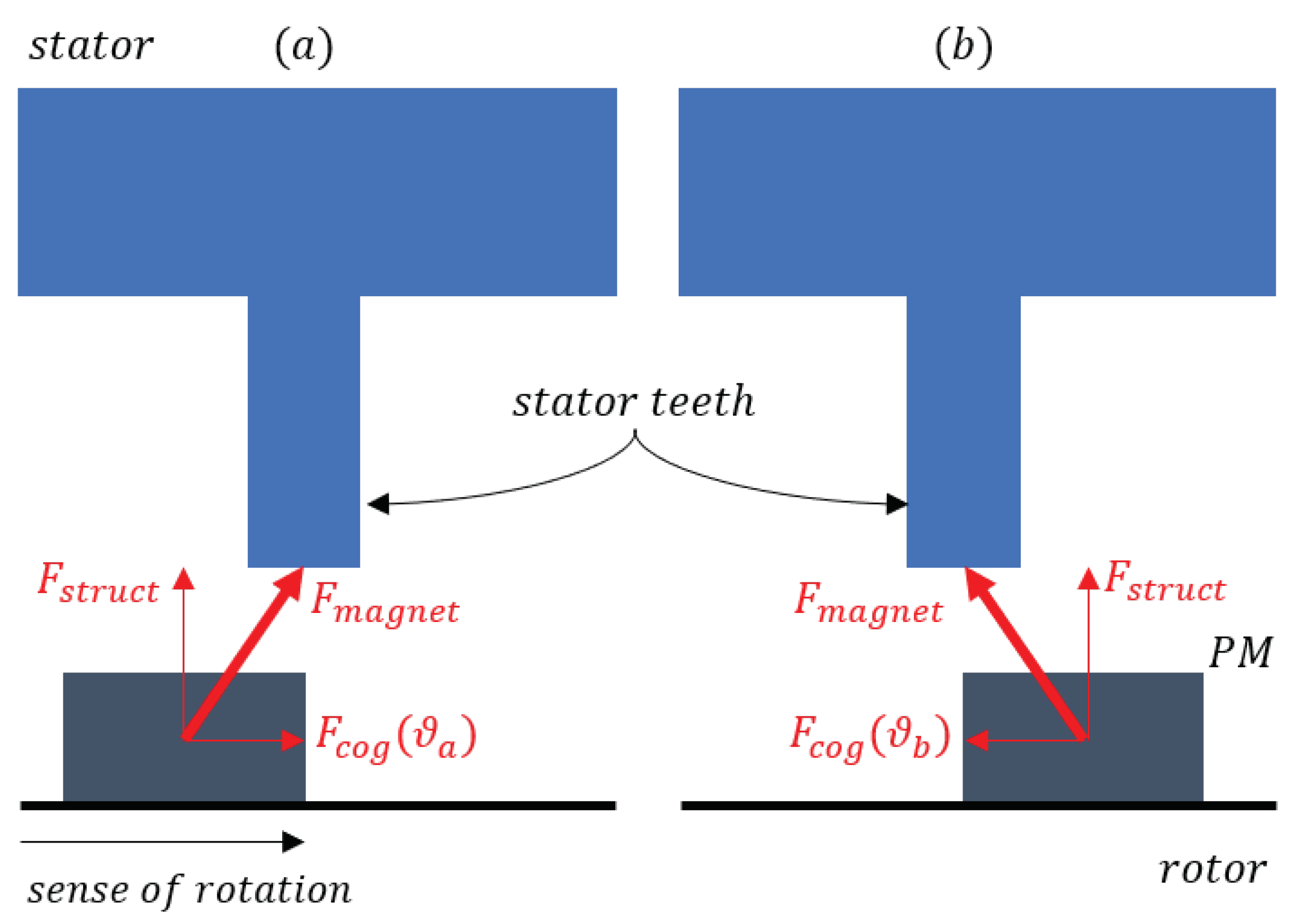
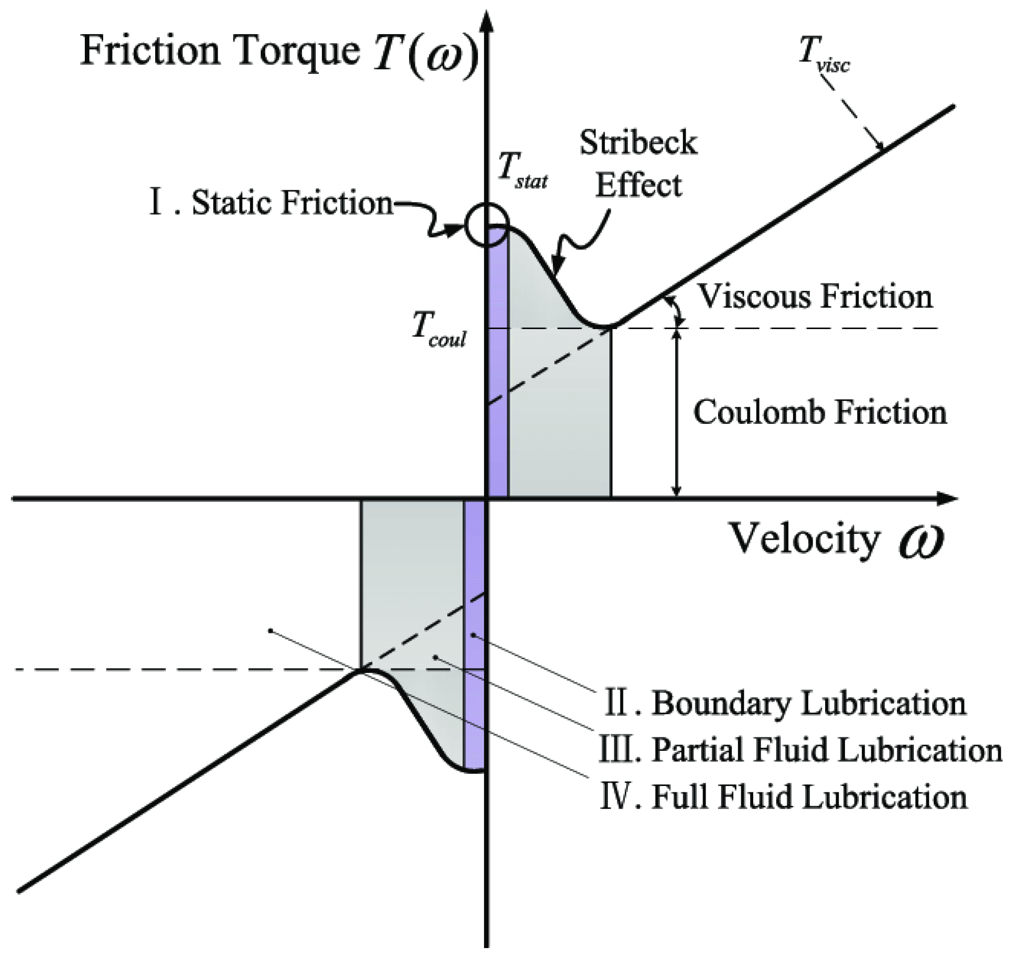
2.1. Brief Explanation of the Cogging and Stribeck Effects
2.2. Related Work
3. System Modelling
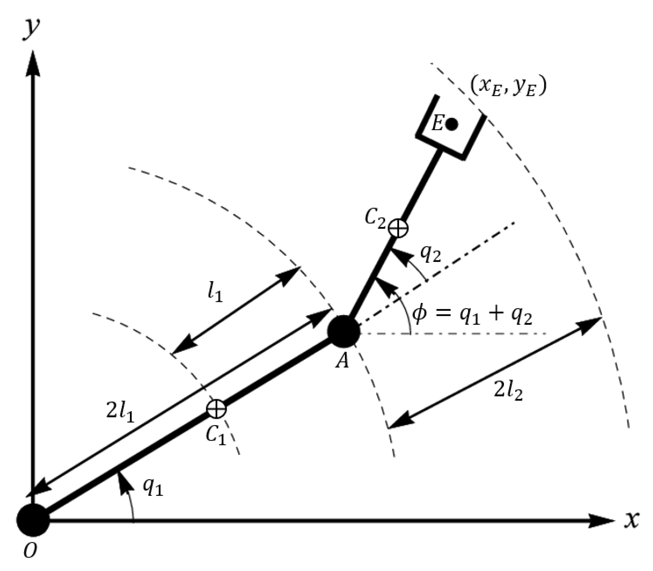
3.1. Robot Dynamics
3.2. Synchronous Motors Modelling
4. Control System Design
4.1. State Space Representation
4.2. Application of the Feedback Linearization Technique
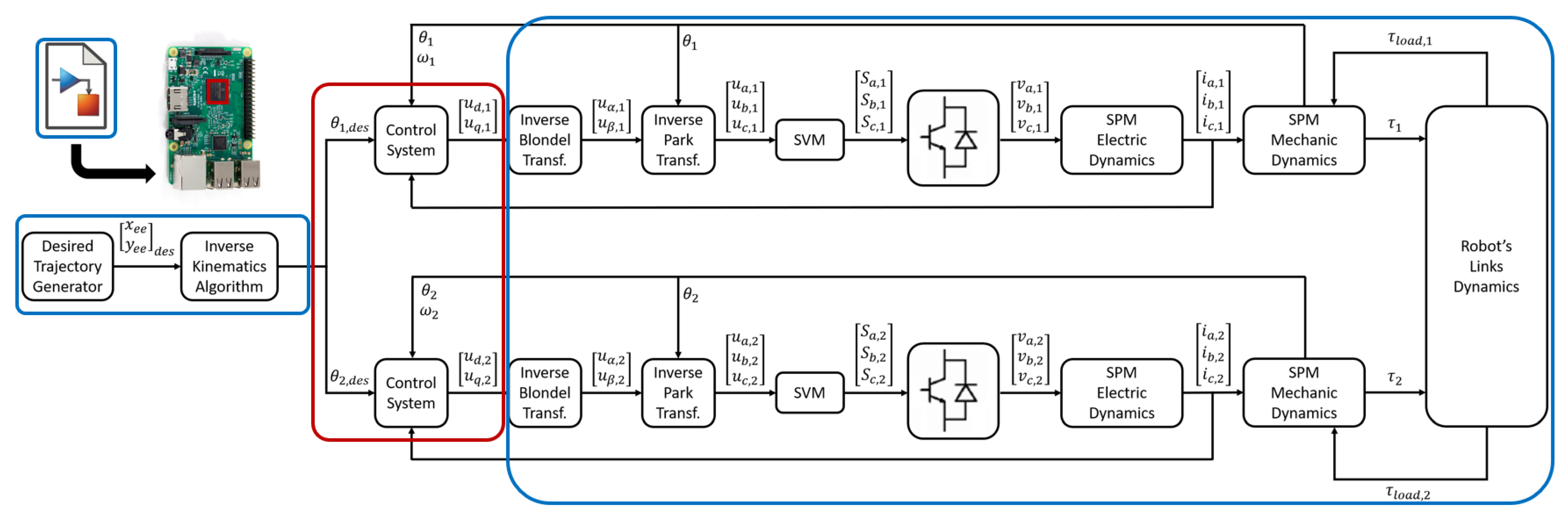
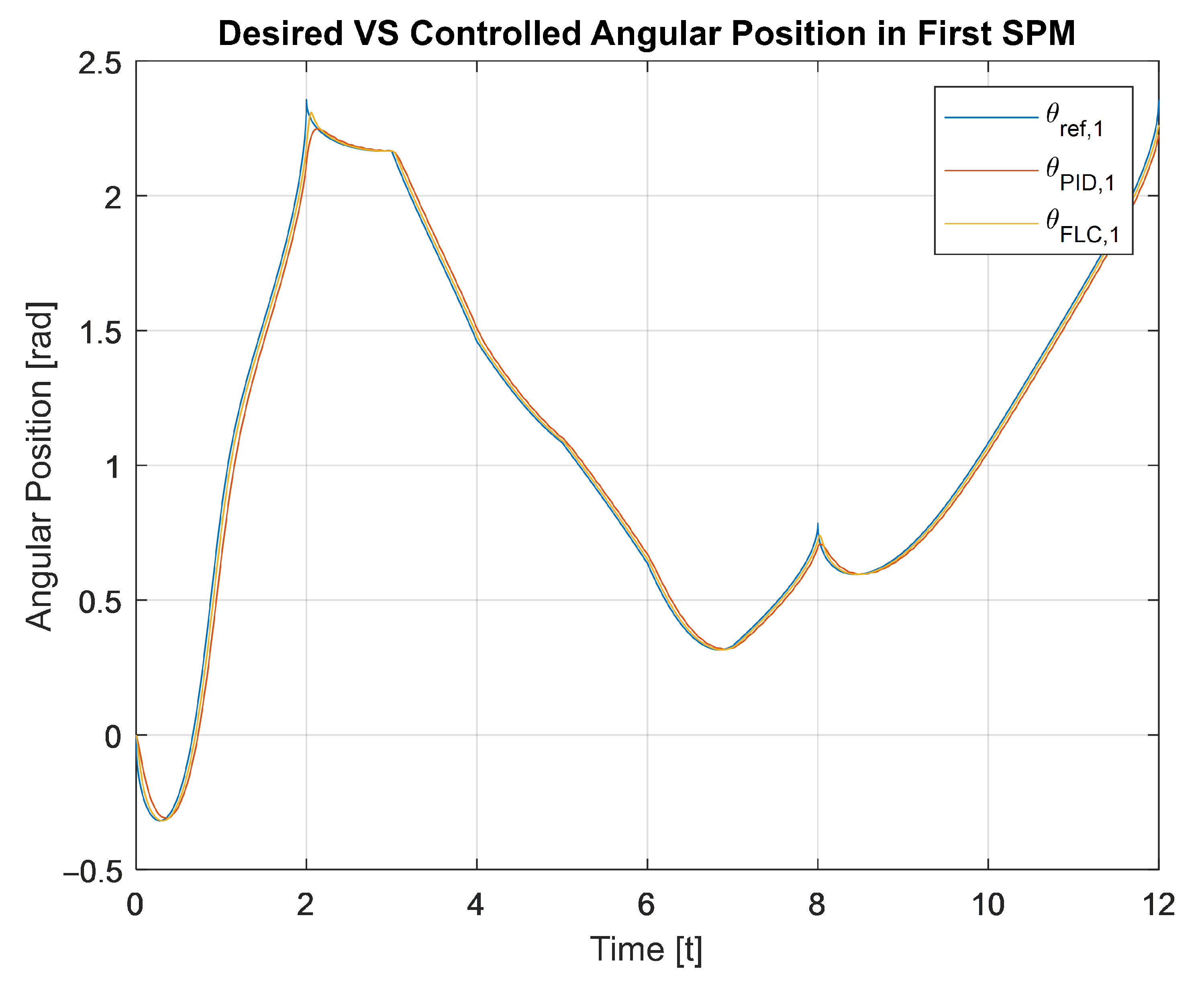
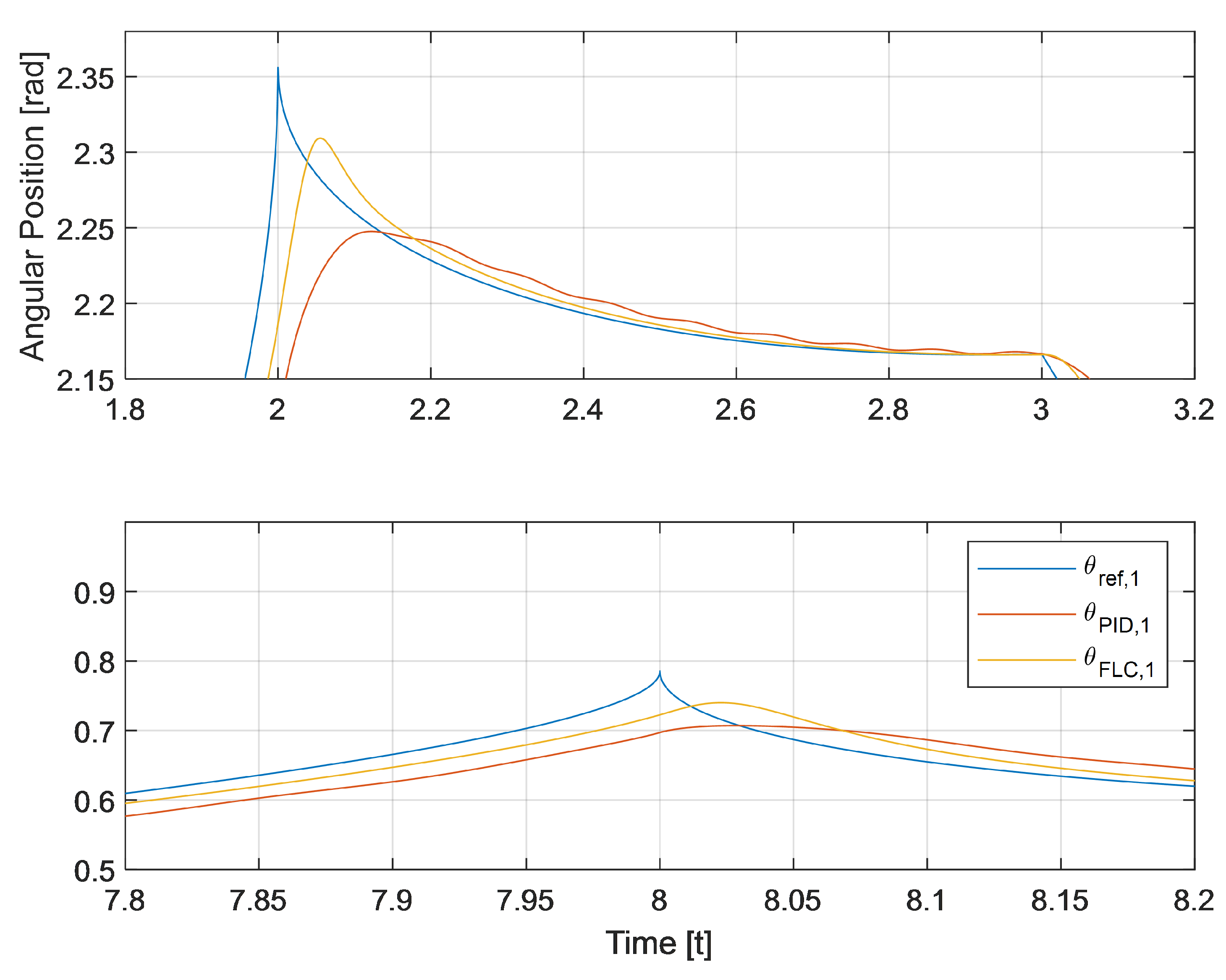
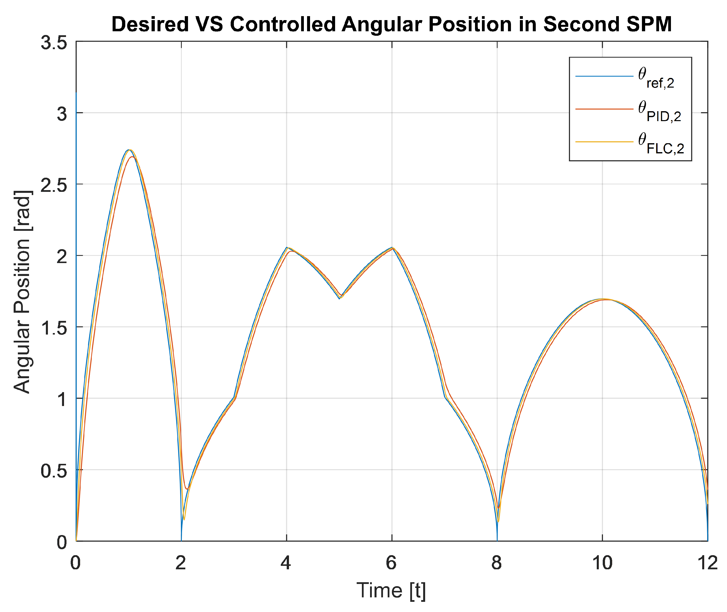
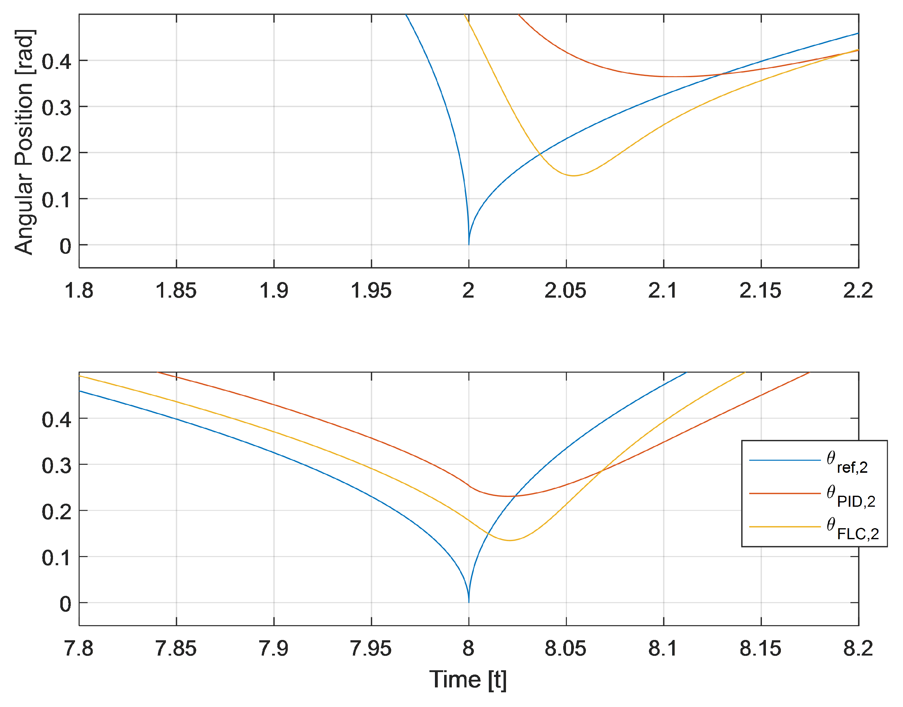
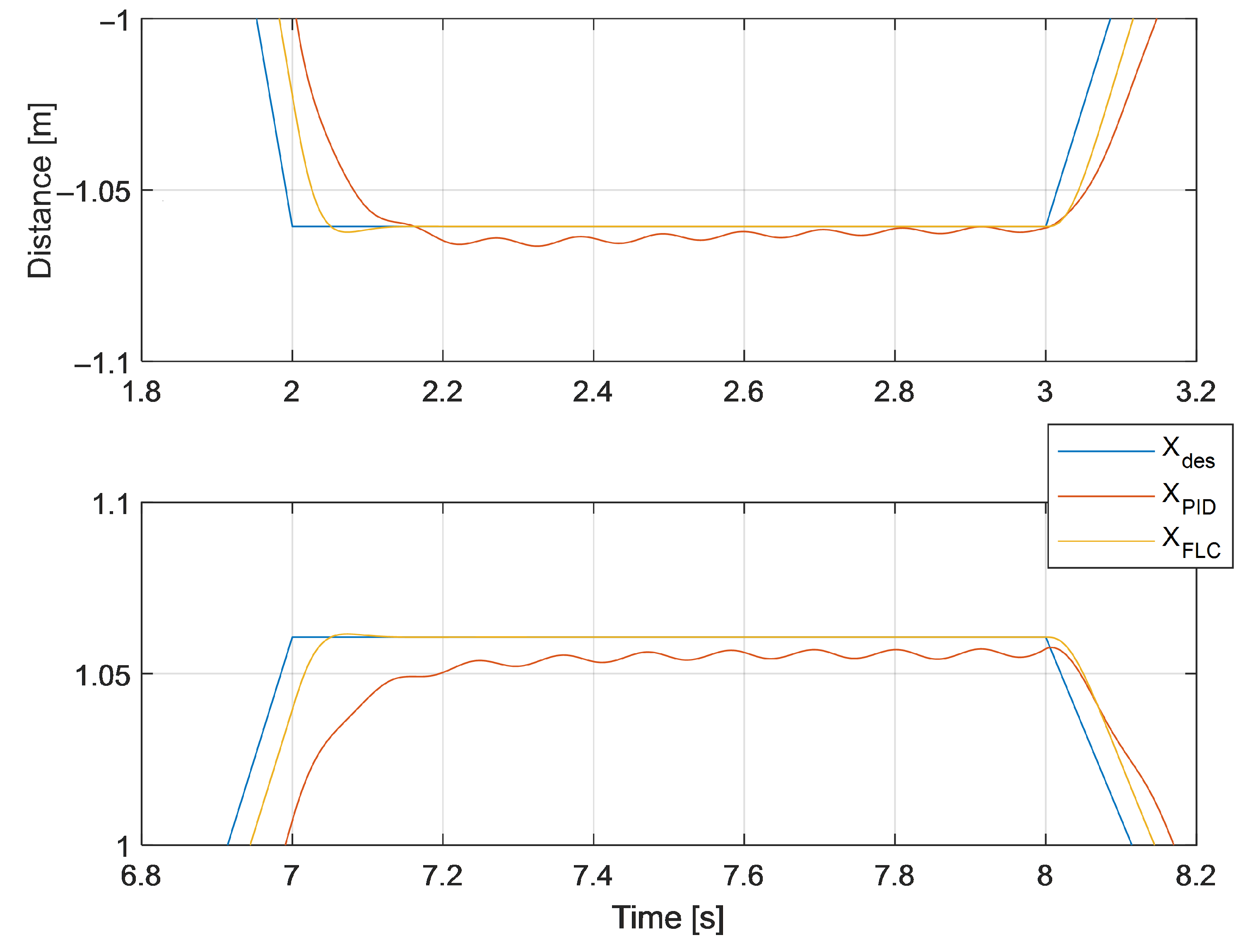
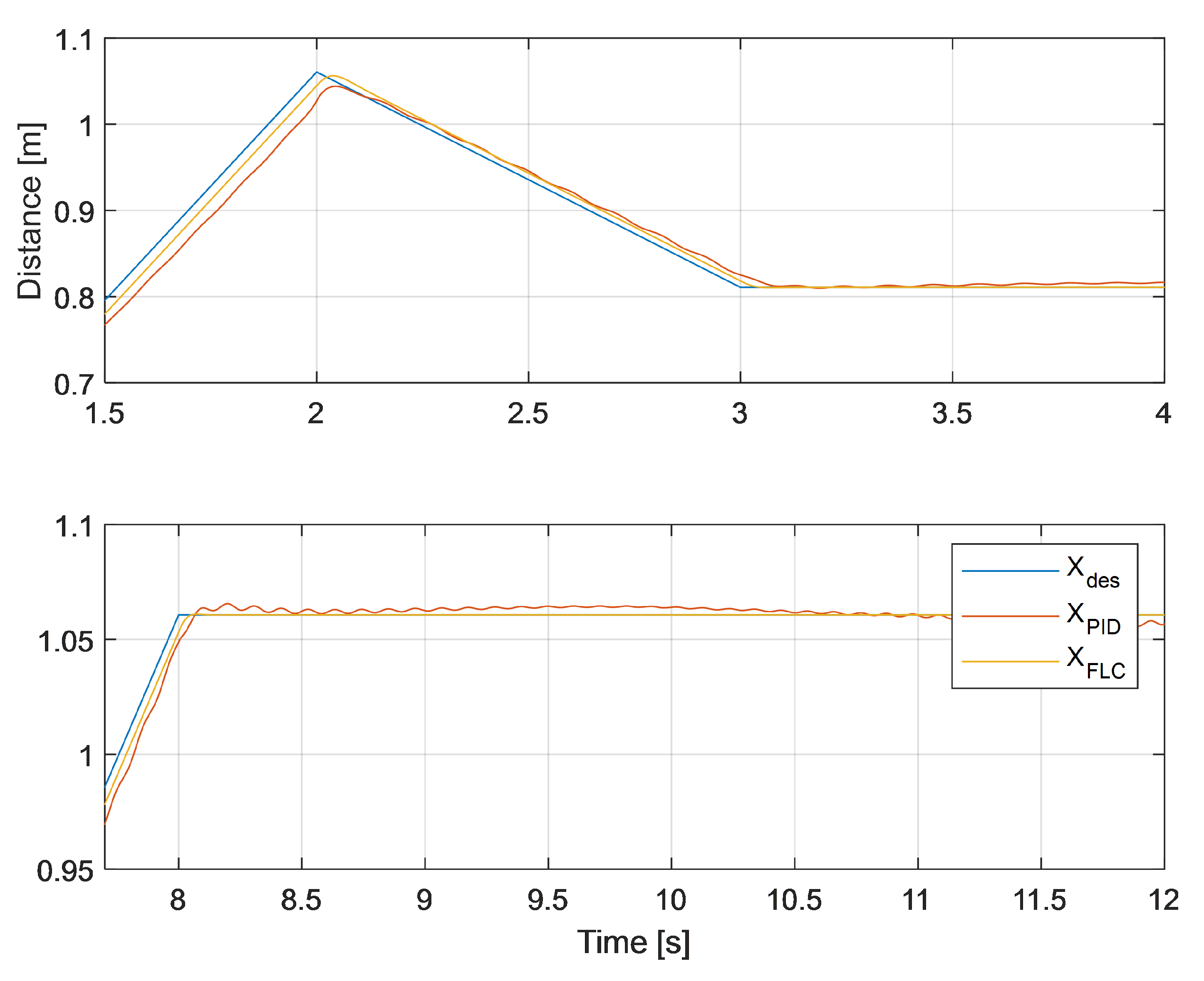
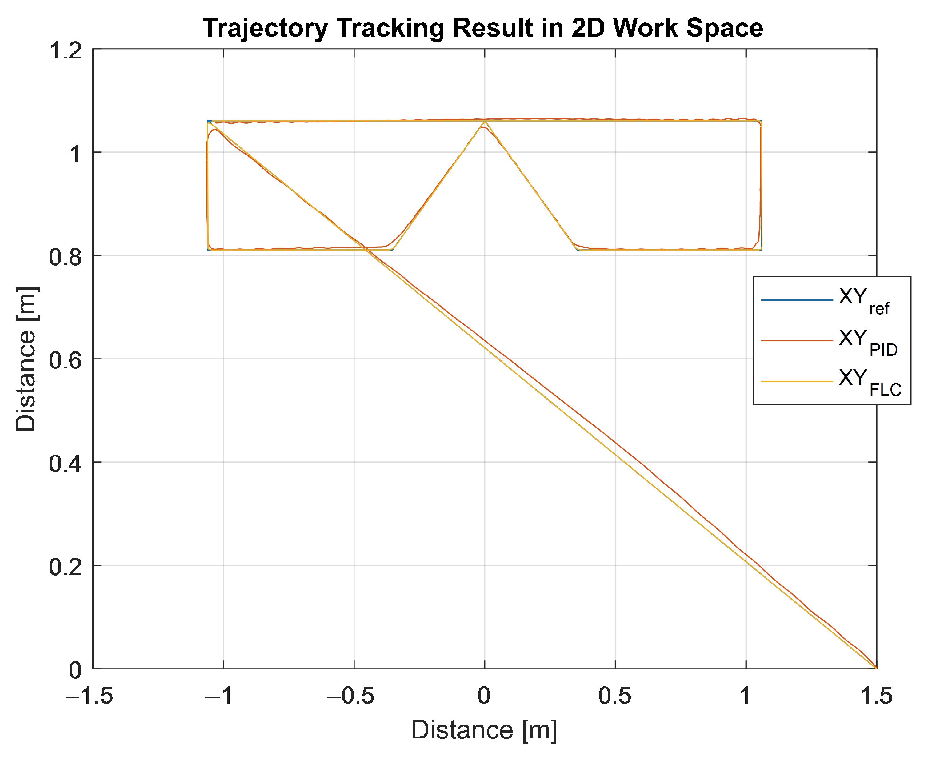
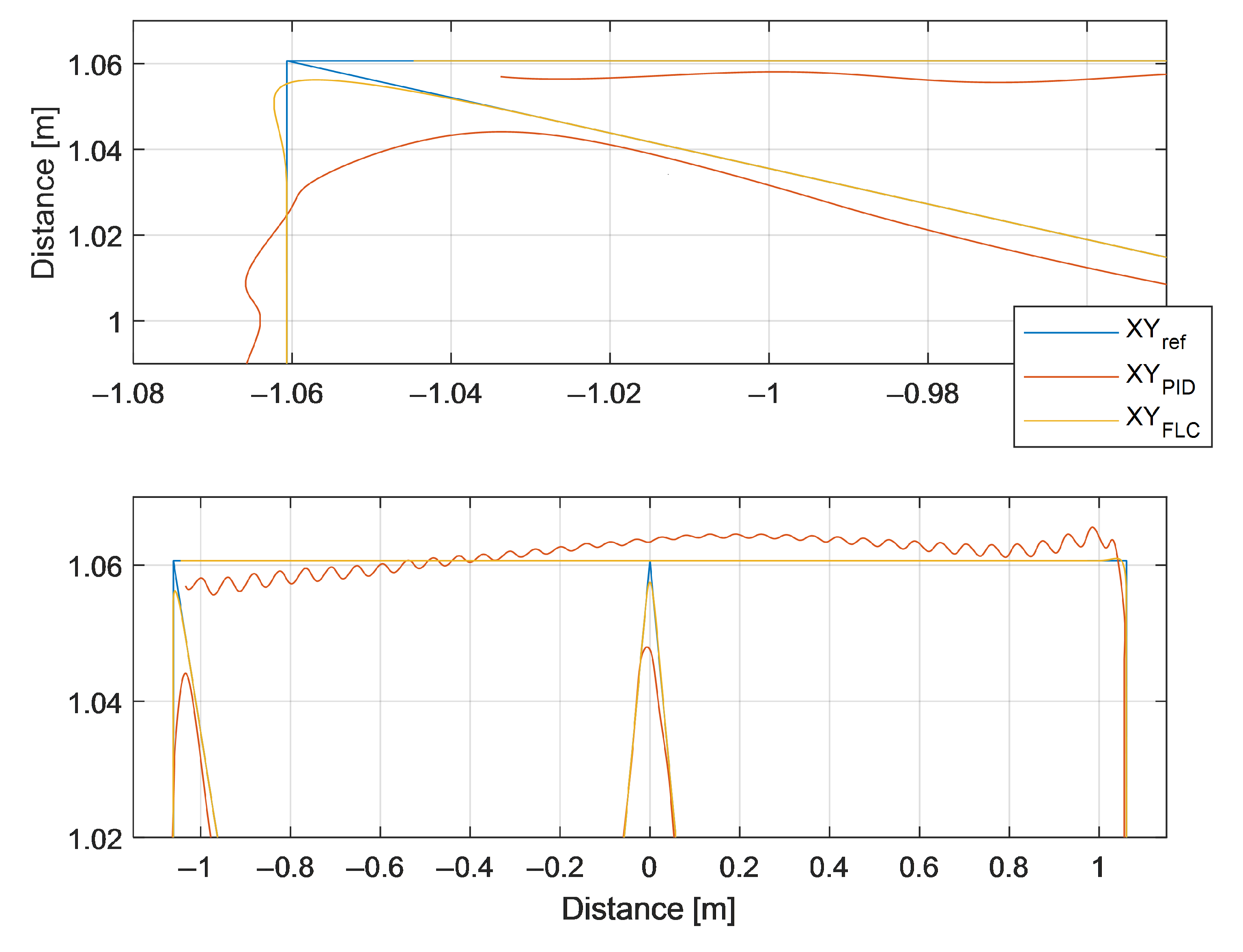
5. Processor-In-the-Loop Simulations
6. Conclusions and Future Work
Author Contributions
Funding
Institutional Review Board Statement
Informed Consent Statement
Data Availability Statement
Conflicts of Interest
References
- Gieras, J.F. Electrical Machines: Fundamentals of Electromechanical Energy Conversion; CRC Press: Boca Raton, FL, USA, 2016. [Google Scholar]
- Ou, J.; Liu, Y.; Qu, R.; Doppelbauer, M. Experimental and theoretical research on cogging torque of PM synchronous motors considering manufacturing tolerances. IEEE Trans. Ind. Electron. 2017, 65, 3772–3783. [Google Scholar] [CrossRef]
- Boroujeni, S.T.; Jalali, P.; Bianchi, N. Analytical modeling of no-load eccentric slotted surface-mounted PM machines: Cogging torque and radial force. IEEE Trans. Magn. 2017, 53, 1–8. [Google Scholar] [CrossRef]
- Shir Guran, A.; Pfeiffer, F.; Popp, K. Dynamics with Friction: Modeling, Analysis and Experiment; World Scientific: Singapore, 2001; Volume 2. [Google Scholar]
- Shi, T.; Cao, Y.; Jiang, G.; Li, X.; Xia, C. A torque control strategy for torque ripple reduction of brushless DC motor with nonideal back electromotive force. IEEE Trans. Ind. Electron. 2017, 64, 4423–4433. [Google Scholar] [CrossRef]
- Shin, S.C.; Choi, C.H.; Youm, J.H.; Lee, T.K.; Won, C.Y. Position control of PMSM using jerk-limited trajectory for torque ripple reduction in robot applications. In Proceedings of the IECON 2012-38th Annual Conference on IEEE Industrial Electronics Society, Montreal, QC, Canada, 25–28 October 2012; pp. 2400–2405. [Google Scholar]
- Shi, T.; Niu, X.; Chen, W.; Xia, C. Commutation torque ripple reduction of brushless DC motor in braking operation. IEEE Trans. Power Electron. 2017, 33, 1463–1475. [Google Scholar] [CrossRef]
- Boroujeni, M.S.; Markadeh, G.A.; Soltani, J. Torque ripple reduction of brushless DC motor based on adaptive input-output feedback linearization. ISA Trans. 2017, 70, 502–511. [Google Scholar] [CrossRef] [PubMed]
- Wang, C.; Wan, Y.; Liang, X. Model establishment with Stribeck friction and fuzzy PID control for Cartesian picking robot system. In Proceedings of the 2017 Chinese Automation Congress (CAC), Jinan, China, 20–22 October 2017; pp. 3070–3074. [Google Scholar]
- Dini, P.; Saponara, S. Design of Adaptive Controller Exploiting Learning Concepts Applied to a BLDC-Based Drive System. Energies 2020, 13, 2512. [Google Scholar] [CrossRef]
- Dini, P.; Saponara, S. Cogging torque reduction in brushless motors by a nonlinear control technique. Energies 2019, 12, 2224. [Google Scholar] [CrossRef] [Green Version]
- Dini, P.; Saponara, S. Design of an observer-based architecture and non-linear control algorithm for cogging torque reduction in synchronous motors. Energies 2020, 13, 2077. [Google Scholar] [CrossRef]
- Bernardeschi, C.; Dini, P.; Domenici, A.; Palmieri, M.; Saponara, S. Formal Verification and Co-Simulation in the Design of a Synchronous Motor Control Algorithm. Energies 2020, 13, 4057. [Google Scholar] [CrossRef]
- Adept. Datasheet Adept Cobra i600 SCARA Robot. Available online: https://manualzz.com/download/10047191 (accessed on 9 October 2021).
- DIRK, J. Introduction to Classical Mechanics: Solutions to Problems; World Scientific: Singapore, 2020. [Google Scholar]
- Hughes, A.; Drury, B. Electric Motors and Drives: Fundamentals, Types and Applications; Newnes: London, UK, 2019. [Google Scholar]
- Gerling, D. Electrical Machines; Springer: Berlin/Heidelberg, Germany, 2016. [Google Scholar]
- Pereira, A.; Althoff, M. Safety control of robots under computed torque control using reachable sets. In Proceedings of the 2015 IEEE International Conference on Robotics and Automation (ICRA), Seattle, WA, USA, 26–30 May 2015; pp. 331–338. [Google Scholar]
- Guo, Q.; Zhang, Y.; Celler, B.G.; Su, S.W. Neural adaptive backstepping control of a robotic manipulator with prescribed performance constraint. IEEE Trans. Neural Netw. Learn. Syst. 2018, 30, 3572–3583. [Google Scholar] [CrossRef] [PubMed]
- Boufadene, M. Nonlinear Control Systems Using MATLAB®; CRC Press: Boca Raton, FL, USA, 2018. [Google Scholar]
- Jang, D.; Choe, G.; Ehsani, M. Vector control of three-phase AC machines: System development in the practice. In Power Systems, 2nd ed.; Springer: Berlin/Heidelberg, Germany, 2015. [Google Scholar]
- Astolfi, A.; Marconi, L. Analysis and Design of Nonlinear Control Systems; Springer: Berlin/Heidelberg, Germany, 2008. [Google Scholar]
- MathWorks. Raspberry Pi Support from Simulink. Available online: https://it.mathworks.com/hardware-support/raspberry-pi-simulink.html (accessed on 9 October 2021).
- Božek, P.; Lozkin, A.; Gorbushin, A. Geometrical method for increasing precision of machine building parts. Procedia Eng. 2016, 149, 576–580. [Google Scholar] [CrossRef] [Green Version]
- RoboteQ. RoboteQ Official Site Web. Available online: https://www.roboteq.com/index.php (accessed on 9 October 2021).
- Curtis Instruments. Curtis Instrument Official Site Web. Available online: https://www.curtisinstruments.com/products/motor-controllers/ (accessed on 9 October 2021).
- IFM Electronic. Processes in Automotive Industry. Available online: https://www.ifm.com/download/files/ifm-processes-in-the-automotive-industry-gb/\protect\T1\textdollarfile/ifm-processes-in-the-automotive-industry-gb.pdf (accessed on 9 November 2021).


| Variables Name | Meaning |
|---|---|
| , | mass of robot’s links |
| , | mass of the Synchronous motors |
| , | inertia moments of the Robot’s links |
| , | inertia moments of the actuator rotors |
| , | semi-lengths of the Robot’s links |
| , | reduction ratios |
| , , , | relatives angular positions and speed |
| , , , | absolutes angular positions and speed |
| Variables Name | Meaning |
|---|---|
| stator resistances | |
| stator inductances | |
| magnetic flux coefficients | |
| pole pairs | |
| friction coefficients | |
| Cogging Torque Fourier Series coefficients | |
| coulomb and static friction torque model | |
| Stribek rotary speed limit | |
| , , , | absolutes angular position and speed |
Publisher’s Note: MDPI stays neutral with regard to jurisdictional claims in published maps and institutional affiliations. |
© 2021 by the authors. Licensee MDPI, Basel, Switzerland. This article is an open access article distributed under the terms and conditions of the Creative Commons Attribution (CC BY) license (https://creativecommons.org/licenses/by/4.0/).
Share and Cite
Dini, P.; Saponara, S. Model-Based Design of an Improved Electric Drive Controller for High-Precision Applications Based on Feedback Linearization Technique. Electronics 2021, 10, 2954. https://doi.org/10.3390/electronics10232954
Dini P, Saponara S. Model-Based Design of an Improved Electric Drive Controller for High-Precision Applications Based on Feedback Linearization Technique. Electronics. 2021; 10(23):2954. https://doi.org/10.3390/electronics10232954
Chicago/Turabian StyleDini, Pierpaolo, and Sergio Saponara. 2021. "Model-Based Design of an Improved Electric Drive Controller for High-Precision Applications Based on Feedback Linearization Technique" Electronics 10, no. 23: 2954. https://doi.org/10.3390/electronics10232954