Multi-Task Learning with Task-Specific Feature Filtering in Low-Data Condition

Abstract

Multi-task learning is a computationally efficient method to solve multiple tasks in one multi-task model, instead of multiple single-task models. MTL is expected to learn both diverse and shareable visual features from multiple datasets. However, MTL performances usually do not outperform single-task learning. Recent MTL methods tend to use heavy task-specific heads with large overheads to generate task-specific features. In this work, we (1) validate the efficacy of MTL in low-data conditions with early-exit architectures, and (2) propose a simple feature filtering module with minimal overheads to generate task-specific features. We assume that, in low-data conditions, the model cannot learn useful low-level features due to the limited amount of data. We empirically show that MTL can significantly improve performances in all tasks under low-data conditions. We further optimize the early-exit architecture by a sweep search on the optimal feature for each task. Furthermore, we propose a feature filtering module that selects features for each task. Using the optimized early-exit architecture with the feature filtering module, we improve the 15.937% in ImageNet and 4.847% in Places365 under the low-data condition where only 5% of the original datasets are available. Our method is empirically validated in various backbones and various MTL settings.

1. Introduction

Convolutional neural networks (CNNs) are nowadays the state-of-the-art methods for a wide range of computer vision tasks, thanks to the large-scale public datasets [1,2,3] and high performance accelerators like graphical processing units (GPUs). For example, CNNs rank the highest in benchmarks in image classification [4,5,6], object detection [7,8,9,10], semantic segmentation [11], and action recognitions [12,13,14]. The general recipe for a successful CNN model includes training a large-sized model with a large-scale dataset. However, the size of a model is usually constrained by the accelerator’s memory, or the training (or inference) speed. Collecting a large-scale dataset is also very expensive. To solve these issues, previous works have proposed multi-task learning (MTL) [12,15,16,17]. By definition, multi-task learning trains a model with multiple functionalities. In the case of a CNN, the backbone feature extractor is shared among multiple tasks, and each task has a task-specific head assigned. Given a single input, the shared backbone extracts a feature map, each task-specific head processes the feature map, and finally multiple outputs are computed for multiple tasks. By sharing the computationally expensive backbone, multi-task learning can be quite effective in saving the computational and parametric costs, in contrast to training multiple models for multiple tasks. One of the early works in multi-task learning, UberNet [18], utilizes task-specific skip connections, combines features across different layers, and computes the task-specific outputs. The network is trained with task-specific losses simultaneously. Another work on multi-task learning, One Model to Learn Them All, has shown that multi-task learning works with heterogeneous tasks such as image classification, machine translation, image captioning and speech recognition. Multi-task learning is also used to improve the target task’s performance by training with auxiliary tasks [19].

Most of the CNNs are trained in a data-driven manner, and that indicates a prerequisite for large-scale datasets. Dataset collection and annotation require a lot of time and financial cost, and a benchmark performance on ImageNet [20] shows that it takes a billion-scale dataset to achieve the state-of-the-art performance. There have been many efforts to make dataset collection more efficient with active learning [21], yet the methods are usually applicable to certain types of tasks such as classification only. At the end of the day, we need to manually collect the dataset, and we have to consider many factors, including the size of the dataset, the privacy issues, the copyrights issues and diversity issues. To annotate a large-scale dataset, some crowd-sourced platforms are used, such as Amazon Mechanical Turk, but it is hard to ensure the quality of the annotations. The quality of the annotations must be checked or refined iteratively. Due to the difficulty in the data collection and annotation, CNN models are usually trained with limited data. In this work, we proposed to utilize a set of such limited data with multi-task learning. The low-data condition is common in real-world scenarios, and let us assume that there are multiple datasets for different tasks. Even though the datasets are collected for different purposes, they share common knowledge, such as low-level image features. Throughout a multi-task learning, the CNN model can better learn such common knowledge with a larger, combined dataset. Thus, multi-task learning can be an effective solution to utilize multiple small-scale datasets, and improve each task’s performance. The efficacy of multi-task learning is empirically validated with multiple sets of small-scale benchmarks.

In this work, we propose a task-specific feature filtering module that does not require heavy task-specific heads to generate task-specific features. Specifically, the feature filtering module learns to select feature channels for each task head in a data-driven manner. Instead of passing the full feature to the task-specific heads, we use a 1-d channel-wise scaling filter to be multiplied to each feature map. The filter is assigned for each task, and the feature filtering is performed right before the task-specific heads. The computational or parametric overhead of this feature filtering module is minimal. Moreover, we are using small task-specific heads, so the overhead over the single-task network is also minimal. Throughout extensive experiments, we validate that the proposed task-specific feature filtering module improves the performance of various multi-task models.

Our main contribution is 2-fold:

• We empirically validate the efficacy of multi-task learning in low-data conditions. The model learns the shared knowledge through multi-task learning from multiple datasets, and eventually improves all task performances over single-task models;
• We propose a simple yet effective way to generate task-specific features, with a task-specific feature filtering module. We consistently yet significantly improved the performances of multi-task models with minimal overhead. With the proposed module, small task-specific heads can exploit the task-specific features with minimal computational costs and high performances.

The remainder of this paper is organized as follows: Section 2 introduces related works. Section 3 includes the descriptions for learning methods, model configurations, and filter configurations. Section 4 introduces the experiment’s results of the proposed method. Section 5 includes the analysis for the experiment’s results. Finally, Section 6 summarizes our methods and results, and Section 7 proposes their limitations and the future directions of our work. sec:RW

2. Related Works

In this section, we investigate previous works related to early-exit architecture, the network architecture we used, and the multi-task learning method we used to merge and train datasets.

2.1. Early-Exit Architecture

Szegedy et al. [22] proposed a network called Inception, creating an exit that outputs directly from a branch in the middle of the network, and proposed a training method in the form of helping back-propagation. In addition, Cai et al. [23] improved the accuracy in object detection by proposing a cascade structure using easy-exit.

However, these methods are not preferred in a situation where the amount of computation and memory are limited because the parameters and computation of the network are improved. Unlike previous studies, Phuong et al. [24] noted that the performance in the early-exit was not significantly different from the performance in the final exit. Therefore, Phuong et al. used the early exit architecture for training in order to prune the model without degrading the accuracy of the network in a situation where the amounts of computation and memory are limited.

Inspired by these studies, we used an early exit architecture to effectively utilize multiple datasets in situations where the size of the dataset is small or the size of the memory is limited. Our early exit architecture infers the results of a different dataset for each exit, and the backbone networks share it.

2.2. Multi-Task Learning

Multi-task learning is a method used in various recognition fields using deep learning such as object detection and instance segmentation. The most well-known application is in object detection, where object localization and object classification are performed simultaneously. Recently, Kim et al. [25] revealed that the performance of object localization is greatly improved if only object localization is performed except for the object classification part in object detection. Kokkinos [18] also found that multi-task learning generally degrades the performance of each task.

On the other hand, Deng et al. [26] improved the performance of face detection by multi-task learning of the task of matching the landmark position of the face and the task of aligning the position of the face bounding box.

As such, multi-task learning is an efficient method to reduce the amount of parameters and computations by sharing backbone networks, but it is a method that may decrease or increase performance depending on the relationship between each task. In order to solve the problem that the performance of each task cannot be preserved in multi-task learning, we propose a method to improve the performance of all tasks by using an early exit architecture.

3. Method

In this section, we introduce the mathematical notation and the necessary background for the discussion of the proposed multi-task training of multi-exit architectures. Then, we discuss the features extracted by training different datasets at the same time, and introduce task-specific feature filtering, a method to efficiently use features in multi-task training with multi-exit architectures.

3.1. Dataset Integration

For multi-task training with multi-exit architectures, we first need to integrate the datasets. For example, to integrate ImageNet and Places365 datasets and merge them into the same mini-batch, the total quantity of these datasets, the size of images, and the number of channels must be considered. In order to match the image size and the number of channels, we fit the smaller image to the larger image size and the number of channels. One-channel images (i.e., grayscale images) are expanded to three channels and are integrated with a dataset consisting of only three RGB channels, and the smaller image size is upsampled through bilinear interpolation to fit the larger size image. In addition, small datasets were oversampled to have the same size as the largest dataset.

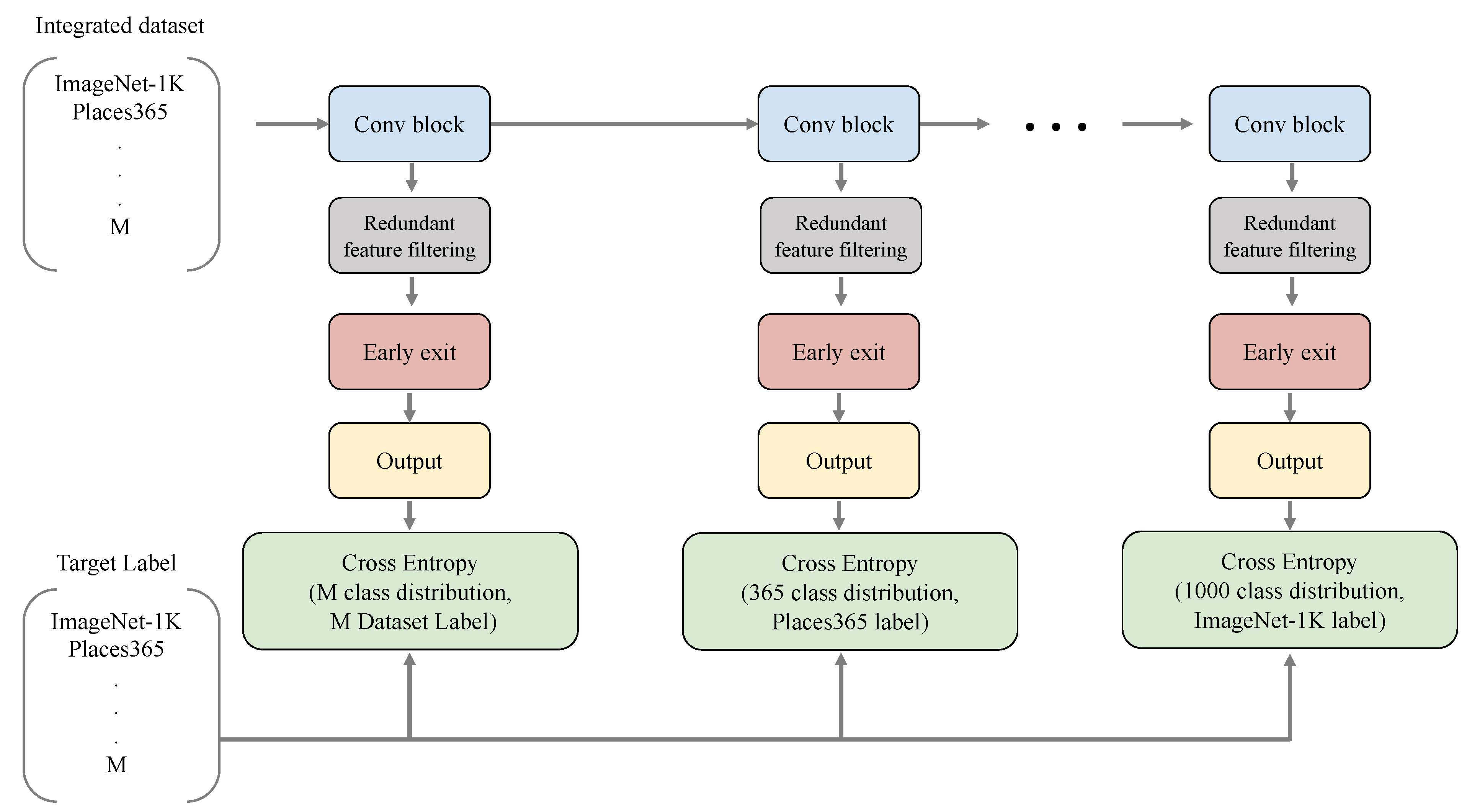
3.2. Multi-Exit Architectures

Our key assumption is that, even in different datasets, the low-level features extracted from the model’s feature extractor can be shared because models for different tasks exhibit similar characteristics [27]. Therefore, if we train with the integrated dataset, the model learns better low-level features due to the increased diversity in the training samples. To further maximize the efficacy of sharing low-level features, we choose early-exit architectures. In early-exit architectures, low-level features are shared among all tasks, and high-level features are not shared.

Early-exit architectures are layered classification architectures with exits at different depths. Figure 1 illustrates a general form of an early-exit architecture. The early-exit architecture has multiple exits, and each exit corresponds to one task. For example, if we merge multiple classification tasks, each exit is a classification network (i.e., multi-layer perceptron) for each task. In order to designate a specific exit for each dataset in the integrated dataset, we sorted the number of classes K in each dataset in ascending order and determined the exit depth according to that order. So, the number of integrated datasets $\left\{1,2,\dots ,m\right\}\in M$ and there is an image and label pair $(x,y)$ for each dataset $D_m$, $x=\left\{x_1,x_2,\dots ,x_N\right\}$, $y\in \left\{1,\dots ,k\right\}$. N is the number of images, and the objective function of multi-exit architectures $f_{\theta }$ can be expressed as follows :

$$\underset{}{min}\frac{1}{M}\frac{1}{N}\sum _{m\in M}\sum _{x,y\in D_m}\left[L_{CE}(f_{\theta }\left(x\right),y)\right].$$

(1)

The final training objective is the sum of all task specific losses. However, please note that labels are only partially available for each training sample. For example, if the training sample is from ImageNet, then only the ImageNet label is available, so we only have the ImageNet cross entropy loss for that sample. The integrated dataset is a balanced combination of multiple datasets, so the minibatch is expected to be sampled from all datasets in a balanced way.

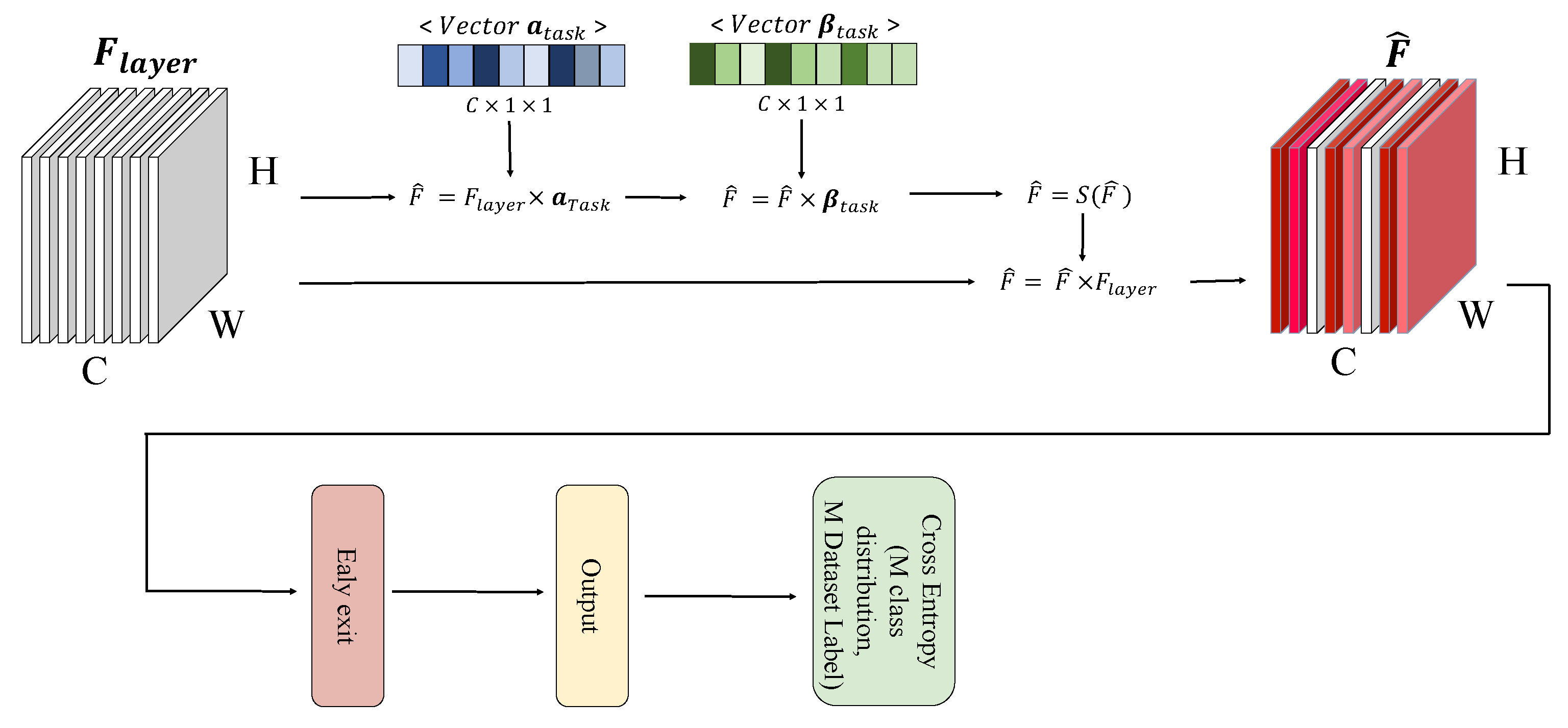
3.3. Task-Specific Feature Filtering

The learned features in MTL are shared and optimized with respect to multiple tasks. The advantage would be learning diverse and sharable features, and the disadvantage would be a lack of task-specific features. Therefore, our assumption is that performance can be improved by generating task-specific features through removing redundant features and inputting them into the classifier rather than naively using the shared features As found in [28], feature filtering can significantly improve the model performances. As revealed in studies [5,28,29,30], features with relatively low activation values are unnecessary or redundant features. Attention mechanisms have been proposed to use this efficiently, but it is difficult to use to remove unnecessary features because it is not performance effective in multi-exit architectures and weights according to attention values without removing features. Therefore, we propose a task-specific feature filtering method that effectively removes unnecessary features for each task-specific exit. The task-specific feature filter module shown in Figure 2 is located before the exit so as not to affect other exits, and is not located in the shared feature extractor. The redundant feature filter has trainable parameters $\alpha$ and $\beta$ that have scalar values as many as the number of input channels when feature F input to each exit is input to the redundant feature filter. $\alpha$ and $\beta$ sequentially perform multiplication and addition operations on the channel. The filter value obtained through this process is adjusted between 0 and 1 through the sigmoid S, and redundant features are removed by multiplying the input features.

This process can be simply expressed in notation as follows:

$$\widehat{F}=F\times S(F\times \alpha +\beta ).$$

(2)

4. Experiments

This section includes the details of the ablation study for searching the optimal multi-exit architecture, and the details of different sets of multiple tasks. The datasets we used for all experiments are in low-data condition, where we uniformly sample the training data. During the uniform sampling, the class distribution is kept the same as the original full dataset. The validation or test datasets remain unchanged. Our experiments are implemented in PyTorch 1.9.0 with NVIDIA RTX3090 (24 G) × 4.

4.1. Multi Task Learning Details

This subsection explains the details of the baseline training settings. VGG [6] and ResNet-50 [31] are chosen as the main backbone architectures throughout this paper. They are the most widely used backbone architectures in the computer vision research community. ResNet is composed of four Layers, and the Layers are composed of multiple convolutional blocks with convolutional layers, batch norm layers, ReLUs, and residual connections. ResNet-50 Layers will have 256, 512, 1024, 2048 channel outputs, respectively. When ResNet-50 is used in a single-task learning (in case of a classification task), the final 2048-channel feature map will be average pooled and classified with the final fully connected layer. Conventional approaches in multi-task learning add heavy task-specific heads in the baseline backbone model with computational and parametric overheads. To reduce the computational overheads, we also search the minimal task-specific heads, where we only use a single fully-connected layer as the task-specific heads. Another design choice for a multi-task model is the exit location.

As discussed in Section 3 Method, different tasks require different levels of semantics. For any task that requires fewer semantics, it will have an earlier exit location, then the other tasks can fully exploit the rest of the computation. As a comprehensive evaluation of multi-task learning in low-data conditions, we compare the effect of heavy task-specific heads and the optimal exit location in a multi-task model. The experiment’s results are included in the Ablation Study section. The final baseline for each experiment’s setting will be chosen after the architecture search with the above factors. The model with the best performance across all tasks will be chosen. For example, in the ImageNet-Places365 experiment, the best setting uses the Layer 4 features for ImageNet classification, and the Layer 3 features for the Places365 classification with the minimal task-specific head of one fully-connected layer.

The hyper-parameters used are as follows. The total number of epochs is 90, the batch size is 256, the base learning rate is 0.1, the learning rate is decayed by 0.1 at epoch 30 and 60 epoch. The validation is done in a single-crop manner in the validation set. We use the overall classification accuracy as the single metric to use. During training, we jointly use all images and labels from the combined dataset with the available label for each image. That is, the images and labels from the ImageNet dataset will be used to compute the cross-entropy loss for the ImageNet task-specific head, and no loss is computed for the Places365 task-specific head, and vice versa. As a result, the multi-task learning baselines improves over the single-task models in all multi-task learning settings by a margin, in all 5%, 10%, 20% low-data settings, with minimal computational overheads over the single-task models.

However, the minimal task-specific heads may not be enough to generate task-specific features as the task-specific heads are very small, and the performance improvements are mostly due to the learned common features with the combined dataset. To further utilize the task-specific features with minimal heads, we propose a task-specific feature filtering module. Details will be explained in the next section.

4.2. Task-Specific Feature Filtering Module Details

In the previous section, we have explained how to compose a strong multi-task model with minimal overheads over the single-task models. However, as the task-specific heads are as minimal as one fully-connected layer, the features used for each task may not be specialized for each task. Therefore, we propose a task-specific feature filtering module that generates task-specific features with minimal overheads yet which are effective in performance improvement. In this section, we explain the proposed task-specific feature filtering module in detail.

The proposed task-specific feature filtering module learns to select useful features for each task in the channel-wise manner. In the module, there are two trainable parameters: a scaling vector and an offset vector. Both vectors are 1D vectors that have the same number of elements with the number of input feature channels. As indicated in the name, the scaling vector will be multiplied to the input features, and the offset vector will be added to the input features, sequentially. The filtered values will be normalized by a Sigmoid layer. The computed values will be normalized within 0 1, and will be used as the final filtering weight to be multiplied to the original input feature map. The computations are all element-wise multiplications, addition, or Sigmoid, so the final overhead is as small as 0.0005G MACs per module. This module is shown to be very effective in multi-task learning; for example, it improves the ImageNet performance by 3.5% and the Places365 performance by 2% in the 5% low-data setting. All the hyper-parameters and the training schemes remain unchanged as the baseline settings found in the previous section.

4.3. Experiment Result

To validate the efficacy of the proposed module, we train models in low-data conditions for ImageNet and Places365 datasets by using 5%, 10% and 20% of the full training set. The methods to be compared are the single-task learning model (STL), the multi-task learning model (MTL), and the multi-task model with our proposed module. In the case of our multi-task learning model, it consists of multiple outlets as shown in Figure 1 In this experiment, our model was constructed by creating exits in Layer 3 and Layer 4. To experiment with our proposed module, our module as shown in Figure 2 was added to each exit of the model as described above. The module we attached has alpha and beta values, respectively, and serves to lower the value of the redundant feature.

As shown in

Table 1. This table is the result of performance comparison experiments for ResNet-50 learned with single task learning (STL) and ResNet-50 learned with multi task learning by our proposed method (Ours MTL). Integration Dataset is a dataset that combines data extracted from ImageNet and Places365 (e.g., 5% Intergration = 5% ImageNet + 5% Places365). The results of each experiment are the inferred results and the accuracy (ACC) between targets.

Training Data	Method	ImageNet ACC (%)	Places365 ACC (%)
5% ImageNet	STL	24.173 ± 1.162	·
5% Places365	STL	·	38.063 ± 1.050
5% Integration	Ours MTL (w/o filtering)	37.064 (+12.891)	40.910 (+2.847)
5% Integration	Ours MTL (w filtering)	40.110 (+15.937)	42.910 (+4.847)
10% ImageNet	STL	48.242 ± 0.585	·
10% Places365	STL	·	43.336 ± 1.211
10% Integration	Ours MTL (w/o filtering)	51.046 (+2.804)	47.095 (+3.430)
10% Integration	Ours MTL (w filtering)	52.656 (+4.414)	47.29 (+3.625)
20% ImageNet	STL	59.765 ± 0.391	·
20% Places365	STL	·	48.007 ± 0.375
20% Integration	Ours MTL (w/o filtering)	61.890 (+2.125)	50.300 (+2.293)
20% Integration	Ours MTL (w filtering)	62.450 (+2.685)	50.843 (+2.836)

, it is shown that the multi-task models have a significantly higher performance than the single-task baseline, and our module further improves significantly over the multi-task models. It is worth noting that the improvement in ImageNet is very significant: the multi-task model improves in ImageNet by 12.891% and the proposed module further improves by 3.046%. The performance improvements are consistently shown across different data conditions.

As shown in

Table 2. The results listed in the table are the results of experimenting with whether our method is useful in combination with ImageNet (IN) and other datasets. It was further learned and tested from the dataset of Oxford Pets (OP) and Caltech-101 (CA). Among the datasets used, the dataset of Caltech-101 was upsampled and tested at a resolution of 224 to match the resolution of ImageNet. All experimental results show that our method could induce performance improvement regardless of the dataset, and that ImageNet’s performance varies slightly depending on the size and task of the dataset.

Training Data	Method	ImageNet	Integration Dataset
		ACC (%)	ACC (%)
5% IN	ResNet50 (STL)	24.173 ± 1.162	·
OP	ResNet50 (STL)	·	70.460
5% IN+OP	Ours MTL (w/o filtering)	32.618 (+8.445)	76.829 (+6.369)
5% IN+OP	Ours MTL (w filtering)	37.396 (+13.223)	85.593 (+15.113)
CA	ResNet50 (STL)	·	74.018
5% IN+CA	Ours MTL (w/o filtering)	26.878 (+2.705)	77.049 (+3.031)
5% IN+CA	Ours MTL (w filtering)	28.192 (+4.019)	85.815 (+11.797)

, we also conducted experiments for ImageNet-Oxford Pets [32], ImageNet-Caltech-101 [33] multi-task settings. The efficacy of the multi-task learning and the proposed module is consistent across different multi-task settings.

Based on the significant improvements over the single-task baselines, we empirically validated the efficacy of multi-task learning in low-data conditions and the efficacy of the proposed task-specific feature filtering module with minimal overheads. Therefore, in low-data conditions, multi-task learning is a very effective method to try with datasets in similar domains but different tasks, and the proposed module is a very cost-effective method to be added.

We verified our method in an additional network. The networks used are SE-ResNet and the VGG 16 Network. In the case of SE-ResNet, we performed Places365 tasks through the feature map output from Layer3, and ImageNet tasks through the feature map output from Layer4 in the same way as ResNet. In the case of the VGG 16 Network, Place365 tasks were performed through the feature map output from the 10th layer, and ImageNet tasks were learned using the feature map output from the 13th layer. Additionally, we used a fully connected layer that extends to 4096 channels before performing the classifier to take advantage of the characteristics of VGG network.

As shown in

Table 3. This table is the result of experimenting with whether it is a method that can be used for other additional architecture. The model we experimented with had a structure of SE-ResNet50 (SE) and VGG-16 (VGG) and conducted a single task learning (STL) experiment, our multi-task learning (MTL) experiment, and an experiment to see if the module had a positive effect on other structures.

Training Data	Method	ImageNet ACC (%)	Places365 ACC (%)
5% ImageNet	SE (STL)	26.188 ± 0.867	·
5% Places365	SE (STL)	·	40.545 ± 0.23
5% Integration	SE (MTL) w/o filtering	38.810 (+12.622)	41.632 (+1.092)
5% Integration	SE (MTL) w filtering	40.201 (+14.013)	42.117 (+1.572)
5% ImageNet	VGG (STL)	27.99 ± 1.095	·
5% Places365	VGG (STL)	·	36.84 ± 0.266
5% Integration	VGG (MTL) w/o filtering	34.406 (+6.416)	40.21 (+3.37)
5% Integration	VGG (MTL) w filtering	35.103 (+7.113)	41.61 (+4.77)

, the result shows that our method is an efficient method in other networks, and that the proposed filtering also further improves performance in our method.

4.4. Multi-Exit Architecture Search

It was necessary to compare the performance of each model to find a combination of features suitable for performing multi-task learning in our structure. Therefore, we performed the task of 10% ImageNet in Layer4 and measured how the inference performance changed according to the combination of Layer1 to Layer4. The model with the exit attached to Layer1 improved the performance of ImageNet compared to the model learned with single task learning, but the performance of Places365 was lower than that learned with single task learning. The model with the exit attached to Layer 2 had the best performance of ImageNet. However, the performance of Places365 was still lower than that of the model learned with single task learning. As shown in

Table 4. This table is the result of the experiment to find the most efficient exit of our method. We created an additional exit on the existing baseline and conducted an experiment using 10% ImageNet and 10% Places365. Additionally, we experimented by creating 4 Layers for ImageNet(STL-ImageNet) and 4 layer for Places365(STL-Places365) in ResNet to proceed with performance comparison with our method(MTL-Layer) and how to do a lot of task specific operations(MTL-Big head).

Method	ImageNet ACC (%)	Places365 ACC (%)	MACs	Parameters
STL-ImageNet	48.242 ± 0.585	·	4.1114G	25.557M
STL-Places365	·	43.336 ± 1.050	4.1114G	25.557M
MTL-Layer4	50.918 (+2.676)	45.820 (+2.484)	4.1123G	26.305M
MTL-Layer3	51.046 (+2.804)	47.095 (+3.759)	4.1119G	25.931M
MTL-Layer2	51.974 (+3.732)	42.670 (−0.666)	4.1120G	25.744M
MTL-Layer1	49.822 (+1.58)	34.361 (−8.975)	4.1123G	25.651M
MTL-Big head	50.090 (+1.848)	46.400 (+3.064)	4.9226G	41.269M
MTL-Layer3 (w filtering)	52.656 (+4.414)	47.290 (+3.954)	4.1120G	25.931M

, we can empirically confirm that the exit model placed in Layer2 produces sacrificial results for the task performed in Layer4. That is, a model in which an exit is attached to Layer2 may enrich the presentation of Layer4. However, multi-task learning does not aim to use the other task sacrificially for one task. Therefore, we did not use the model in which the exit was placed in Layer2. The model in which the exit was placed in Layer3 had lower ImageNet performance than the model in which the exit was placed in Layer2, but the performance in Places365 was the best at 47.095%.

It is important to maximize both tasks’ performances with MTL. Therefore, as a result, we have chosen to use Layer3 features and Layer4 features for the two tasks respectively. The model in which the exit was placed in Layer4 with an exit at Layer4 had lower performances in all tasks than the model with an exit at Layer3. In addition, it was not selected as our architecture because it accounts for the highest percentage of memory and computing sources among the models experimented so far. We additionally conducted the experiment by adding one more Layer4 to the existing ResNet, inspired by the fact that existing multi-task learning creates task specific features. As a result, although MACs and parameters were the highest among the models we tested, ImageNet performance was the second worst among the models we tested, and Places365 performance did not exceed that of the model placed on Layer3. Therefore, it was confirmed that it was not helpful to unconditionally add a large amount of computation to generate task specific features. As the last experiment, we experimented with the filtering we suggested. We confirmed that our filtering adds fewer MACs and parameters and can show a better performance than baseline models.

5. Analysis

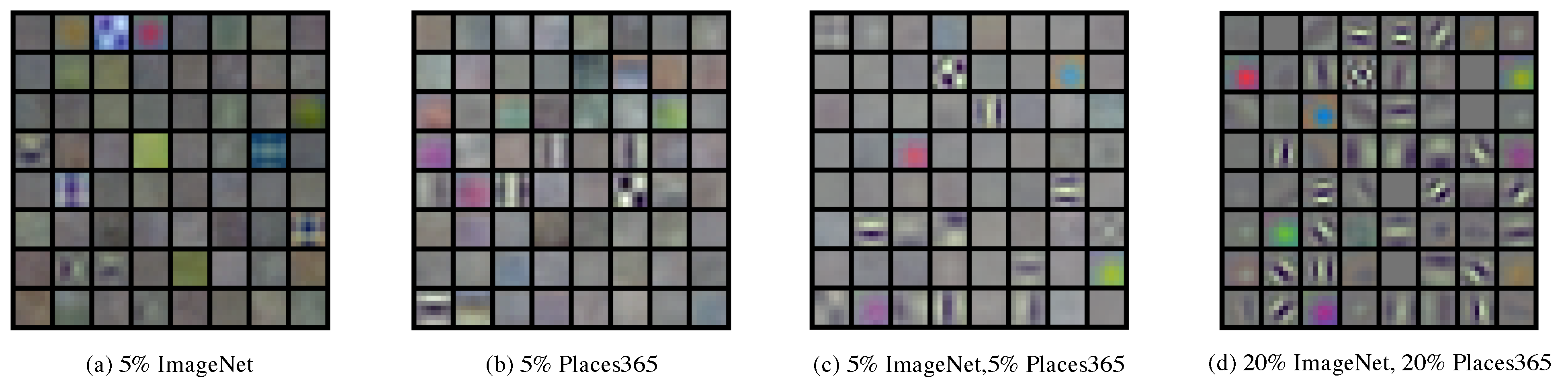
5.1. Multi-Exit Architectures with Filter Visualization

The weight value of the first convolution filter of ResNet-50 is visualized as shown in Figure 3 to see if our proposed multi-task learning method can generate more diverse convolution filters. We compared all ImageNet images based on the weight of the filter of the model in which we have learned for a more accurate visual comparison of our multitasking learning architecture and single task learning architecture. The filter value of the model in which only 5% of the ImageNet was learned showed the worst results when compared with the filter value of the model in which all of ImageNet was learned. In 5% Places365 with more data than 5% ImageNet, it was confirmed that the 5% ImageNet model had more diverse filters. Finally, in the case of our multi-task architecture, when we learned that, by fusing a dataset of 5%, it can be seen that the values of the filters have become more diverse and complex. Thus, the model learned by our method may have more diverse and complex filters than the method of the single task method.

5.2. Visualization of the Distribution of Feature Filtering Values

Our proposed module is trained to reduce the value of unnecessary features in task-specific features. We calculated and visualized the fixed $\alpha$ value and $\beta$ value after learning exists in the module to see if the module is performing filtering of redundant features as learning progresses. The values consisting of red dots in Figure 4 come from our module when $\alpha$ and $\beta$ values pass through sigmoid, and many values are distributed in 0.5 and 0.65. In other words, it can be seen that the location of an insignificant channel and the location of an important channel are classified. We visualized the features entered and the output features to see how these values change when the features generated in our model are received as inputs. It was confirmed how the 777th input channel with the highest a value and 685th input channel with the lowest value of the learned module changed when they passed through the module, respectively.

As a result, the values of the 777th channel were generated very similarly to the values of the input feature, and the values of the 685th channel were output with the values of the channel decreasing. With these experiments, we identifyied channels where the modules we proposed were not important, and we were able to help improve performance as previously tested.

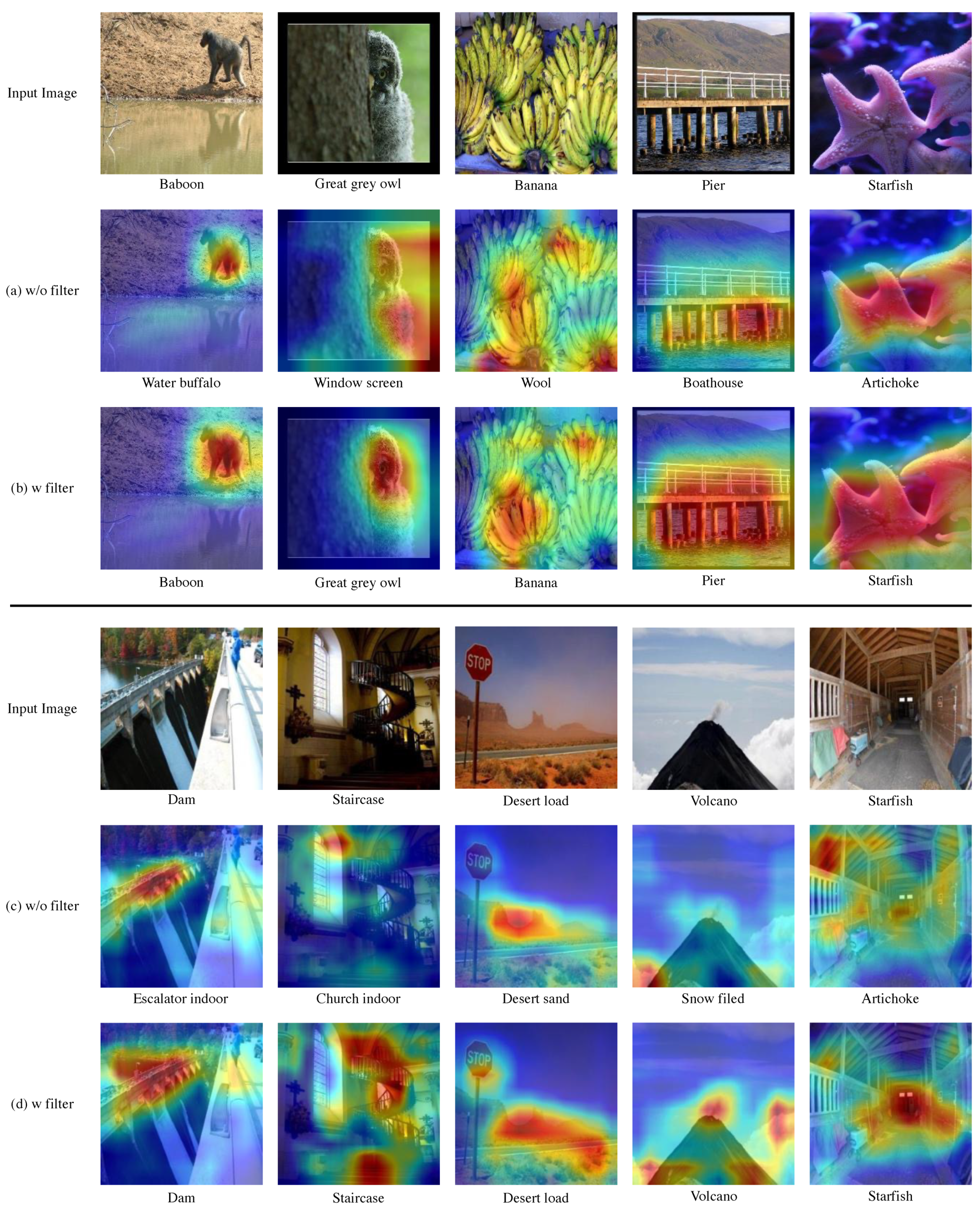
5.3. Redundant Feature Filtering Visualization with Grad-CAM

Our proposed filtering is shown to be efficient in our proposed multi-task learning method. In order to check how our filtering affects the model, Grad-CAM [34] was used to check which part of the input image the model with and without filtering observed and predicted. The image used in the result is a validation image of ImageNet and an unlearned sample.

In the case of predicting through a model without filtering in the ImageNet task, the location of the object was not accurately identified as shown in Figure 5a, or even if it was identified, the prediction was attempted only through some areas in the object. For example, when it was necessary to predict ’Pier’, the entire information of the pier was not identified, and only the area where the pier and the river meet was judged, resulting in a wrong result of ’bathhouse’. However, for models learned by adding our modules, we were able to make more improved predictions by using the area information of the object present in the image more widely.

In the Place365 task, models without filtering were predicted using fewer areas. In other words, as shown in Figure 5c, the information on the background, which generally exists in the area of the image, was not fully utilized. However, in the case of our model, we were able to make more improved predictions using a wider area of the image compared to a model without filtering.

6. Conclusions

In this work, we have validated the efficacy of multi-task learning in low-data conditions, and proposed a cost-effective feature filtering module to generate task-specific features with minimal overheads. Our main target is the low-data conditions, so we used 5%, 10%, and 20% of public benchmark training datasets as the training datasets. Among various design options for multi-task models, we focus on the early-exit options and the size of the task-specific heads. Apart from the conventional methods, we discovered that minimal task-specific heads can be more effective than heavy task-specific heads with proper choices of early-exit in the backbone feature extractor. Furthermore, we propose a task-specific feature filtering module to exploit task-specific features for the minimal task-specific heads. As a result, we have shown a structured approach to designing models for multi-task learning, and have shown that the proposed module is effective in all tasks in all low-data conditions. The future direction of this research would be an extension to more various tasks, such as segmentation and detection. The multi-task learning among multiple segmentation tasks, or among segmentation and classification tasks is to be discovered.

7. Future Work

In our work, multi-dataset integration, MTL and redundant feature filtering methods were validated and demonstrated in the image classification task. However, the extremely small data scenario can occur in various tasks such as semantic segmentation [35,36,37] and object detection as well as image classification problems. Since our method is not an architecture limited to image classification tasks, it can be easily extended by selecting a multi-exit architecture suitable for each task, such as [38] in semantic segmentation and [23] in object detection. Redundant feature filtering also has room for improvement by applying an attention method such as that in [4,9]. Therefore, in our future work, we plan to apply and verify our method in various computer vision problems.

References

1. Shao, S.; Li, Z.; Zhang, T.; Peng, C.; Yu, G.; Zhang, X.; Li, J.; Sun, J. Objects365: A Large-Scale, High-Quality Dataset for Object Detection. In Proceedings of the 2019 IEEE/CVF International Conference on Computer Vision (ICCV), Seoul, Korea, 27 October–2 November 2019; pp. 8429–8438. [Google Scholar]
2. Zhou, B.; Khosla, A.; Lapedriza, A.; Torralba, A.; Oliva, A. Places: An image database for deep scene understanding. arXiv 2016, arXiv:1610.02055. [Google Scholar] [CrossRef]
3. Cordts, M.; Omran, M.; Ramos, S.; Rehfeld, T.; Enzweiler, M.; Benenson, R.; Franke, U.; Roth, S.; Schiele, B. The Cityscapes Dataset for Semantic Urban Scene Understanding. In Proceedings of the IEEE Conference on Computer Vision and Pattern Recognition, Las Vegas, NV, USA, 26–30 June 2016. [Google Scholar]
4. Wu, Y.; Mu, G.; Qin, C.; Miao, Q.; Ma, W.; Zhang, X. Semi-supervised hyperspectral image classification via spatial-regulated self-training. Remote Sens. 2020, 12, 159. [Google Scholar] [CrossRef] [Green Version]
5. Hu, J.; Shen, L.; Sun, G. Squeeze-and-excitation networks. In Proceedings of the IEEE Conference on Computer Vision and Pattern Recognition, Salt Lake City, UT, USA, 18–23 June 2018; pp. 7132–7141. [Google Scholar]
6. Simonyan, K.; Zisserman, A. Very deep convolutional networks for large-scale image recognition. arXiv 2014, arXiv:1409.1556. [Google Scholar]
7. Ren, S.; He, K.; Girshick, R.; Sun, J. Faster r-cnn: Towards real-time object detection with region proposal networks. Adv. Neural Inf. Process. Syst. 2015, 28, 91–99. [Google Scholar] [CrossRef] [PubMed] [Green Version]
8. Redmon, J.; Farhadi, A. Yolov3: An incremental improvement. arXiv 2018, arXiv:1804.02767. [Google Scholar]
9. Wu, Y.; Bai, Z.; Miao, Q.; Ma, W.; Yang, Y.; Gong, M. A classified adversarial network for multi-spectral remote sensing image change detection. Remote Sens. 2020, 12, 2098. [Google Scholar] [CrossRef]
10. Hasan, M.K.; Ahsan, M.; Newaz, S.; Lee, G.M.; Abdullah-Al-Mamun. Human face detection techniques: A comprehensive review and future research directions. Electronics 2021, 10, 2354. [Google Scholar] [CrossRef]
11. Chen, L.C.; Papandreou, G.; Schroff, F.; Adam, H. Rethinking atrous convolution for semantic image segmentation. arXiv 2017, arXiv:1706.05587. [Google Scholar]
12. Xu, Y.; Zhou, F.; Wang, L.; Peng, W.; Zhang, K. Optimization of Action Recognition Model Based on Multi-Task Learning and Boundary Gradient. Electronics 2021, 10, 2380. [Google Scholar] [CrossRef]
13. Carreira, J.; Zisserman, A. Quo vadis, action recognition? A new model and the kinetics dataset. In Proceedings of the IEEE Conference on Computer Vision and Pattern Recognition, Honolulu, HI, USA, 21–26 June 2017; pp. 6299–6308. [Google Scholar]
14. Simonyan, K.; Zisserman, A. Two-stream convolutional networks for action recognition in videos. arXiv 2014, arXiv:1406.2199. [Google Scholar]
15. Caruana, R. Multitask learning. Machine learning 1997, 28, 41–75. [Google Scholar] [CrossRef]
16. Kaiser, L.; Gomez, A.N.; Shazeer, N.M.; Vaswani, A.; Parmar, N.; Jones, L.; Uszkoreit, J. One Model To Learn Them All. arXiv 2017, arXiv:abs/1706.05137. [Google Scholar]
17. Li, J.; Zhang, D.; Ma, Y.; Liu, Q. Lane Image Detection Based on Convolution Neural Network Multi-Task Learning. Electronics 2021, 10, 2356. [Google Scholar] [CrossRef]
18. Kokkinos, I. UberNet: Training a Universal Convolutional Neural Network for Low-, Mid-, and High-Level Vision Using Diverse Datasets and Limited Memory. In Proceedings of the IEEE Conference on Computer Vision and Pattern Recognition, Honolulu, HI, USA, 21–26 June 2017; pp. 5454–5463. [Google Scholar]
19. Mirowski, P.W.; Pascanu, R.; Viola, F.; Soyer, H.; Ballard, A.; Banino, A.; Denil, M.; Goroshin, R.; Sifre, L.; Kavukcuoglu, K.; et al. Learning to Navigate in Complex Environments. ArXiv 2017, abs/1611.03673. [Google Scholar]
20. Deng, J.; Dong, W.; Socher, R.; Li, L.J.; Li, K.; Fei-Fei, L. ImageNet: A large-scale hierarchical image database. In Proceedings of the 2009 IEEE Conference on Computer Vision and Pattern Recognition, Miami, FL, USA, 20–25 June 2009; pp. 248–255. [Google Scholar] [CrossRef] [Green Version]
21. Cohn, D.A.; Ghahramani, Z.; Jordan, M.I. Active learning with statistical models. J. Artif. Intell. Res. 1996, 4, 129–145. [Google Scholar] [CrossRef]
22. Szegedy, C.; Liu, W.; Jia, Y.; Sermanet, P.; Reed, S.; Anguelov, D.; Erhan, D.; Vanhoucke, V.; Rabinovich, A. Going deeper with convolutions. In Proceedings of the IEEE Conference on Computer Vision and Pattern Recognition, Boston, MA, USA, 7–12 June 2015; pp. 1–9. [Google Scholar]
23. Cai, Z.; Vasconcelos, N. Cascade r-cnn: Delving into high quality object detection. In Proceedings of the IEEE Conference on Computer Vision and Pattern Recognition, Salt Lake City, UT, USA, 18–23 June 2018; pp. 6154–6162. [Google Scholar]
24. Phuong, M.; Lampert, C.H. Distillation-based training for multi-exit architectures. In Proceedings of the IEEE/CVF International Conference on Computer Vision, Seoul, Korea, 27–28 October 2019; pp. 1355–1364. [Google Scholar]
25. Kim, D.; Lin, T.Y.; Angelova, A.; Kweon, I.S.; Kuo, W. Learning Open-World Object Proposals without Learning to Classify. arXiv 2021, arXiv:2108.06753. [Google Scholar]
26. Deng, J.; Guo, J.; Zhou, Y.; Yu, J.; Kotsia, I.; Zafeiriou, S. Retinaface: Single-stage dense face localisation in the wild. arXiv 2019, arXiv:1905.00641. [Google Scholar]
27. Zeiler, M.D.; Fergus, R. Visualizing and understanding convolutional networks. In European Conference on Computer Vision; Springer: Berlin/Heidelberg, Germany, 2014; pp. 818–833. [Google Scholar]
28. Seo, M.; Lee, J.; Park, J.; Kim, D.; Choi, D.G. Sequential Feature Filtering Classifier. IEEE Access 2021, 9, 97068–97078. [Google Scholar] [CrossRef]
29. Woo, S.; Park, J.; Lee, J.Y.; Kweon, I.S. Cbam: Convolutional block attention module. In Proceedings of the European Conference on Computer Vision (ECCV), Munich, Germany, 8–14 September 2018; pp. 3–19. [Google Scholar]
30. Ma, W.; Zhao, J.; Zhu, H.; Shen, J.; Jiao, L.; Wu, Y.; Hou, B. A Spatial-Channel Collaborative Attention Network for Enhancement of Multiresolution Classification. Remote Sens. 2021, 13, 106. [Google Scholar] [CrossRef]
31. He, K.; Zhang, X.; Ren, S.; Sun, J. Deep residual learning for image recognition. In Proceedings of the IEEE Conference on Computer Vision and Pattern Recognition, Las Vegas, NV, USA, 26–30 June 2016; pp. 770–778. [Google Scholar]
32. Parkhi, O.M.; Vedaldi, A.; Zisserman, A.; Jawahar, C. Cats and dogs. In Proceedings of the 2012 IEEE Conference on Computer Vision and Pattern Recognition, Washington, DC, USA, 16–21 June 2012; pp. 3498–3505. [Google Scholar]
33. Fei-Fei, L.; Fergus, R.; Perona, P. Learning generative visual models from few training examples: An incremental bayesian approach tested on 101 object categories. In Proceedings of the 2004 Conference on Computer Vision and Pattern Recognition Workshop, Washington, DC, USA, 27 June–2 July 2004; p. 178. [Google Scholar]
34. Selvaraju, R.R.; Cogswell, M.; Das, A.; Vedantam, R.; Parikh, D.; Batra, D. Grad-cam: Visual explanations from deep networks via gradient-based localization. In Proceedings of the IEEE International Conference on Computer Vision, Venice, Italy, 22–29 October 2017; pp. 618–626. [Google Scholar]
35. Kang, D.; Wong, A.; Lee, B.; Kim, J. Real-Time Semantic Segmentation of 3D Point Cloud for Autonomous Driving. Electronics 2021, 10, 1960. [Google Scholar] [CrossRef]
36. Garcia-Ortiz, L.B.; Portillo-Portillo, J.; Hernandez-Suarez, A.; Olivares-Mercado, J.; Sanchez-Perez, G.; Toscano-Medina, K.; Perez-Meana, H.; Benitez-Garcia, G. FASSD-Net Model for Person Semantic Segmentation. Electronics 2021, 10, 1393. [Google Scholar] [CrossRef]
37. Ouahabi, A.; Taleb-Ahmed, A. Deep learning for real-time semantic segmentation: Application in ultrasound imaging. Pattern Recognit. Lett. 2021, 144, 27–34. [Google Scholar] [CrossRef]
38. Chen, L.C.; Papandreou, G.; Kokkinos, I.; Murphy, K.; Yuille, A.L. Deeplab: Semantic image segmentation with deep convolutional nets, atrous convolution, and fully connected crfs. IEEE Trans. Pattern Anal. Mach. Intell. 2017, 40, 834–848. [Google Scholar] [CrossRef] [PubMed]
Figure 1. Multi-exit architectures for multi-task learning. There are as many exits as M, which is the number of integrated datasets, and the order is determined according to the number of classes in each dataset.
Electronics 10 02691 g001
Figure 2. It is a schematic figure of the changes that occur when the input feature passes through our module. The input feature is used as an input of the exit by making the values of channels that are not helpful for the task into small values.
Electronics 10 02691 g002
Figure 3. This figure illustrates how various low level features can be created by the model learned by the method we proposed. Each figure is the weight of the convolutional filter that first exists in ResNet-50. (a) is the filter of the model with 5% ImageNet and single task learning. (b) is the filter of the model with 5% Places365 and single task learning. (c) is the filter of the model that fused 5% ImageNet and 5% Places365 to perform multi-task learning in our way. (d) is the filter of the model that fused 20% ImageNet and 20% Places365 to perform multi-task learning in our way.
Electronics 10 02691 g003
Figure 4. It is a picture depicting actual features changing with modules learned on 5% ImageNet and 5% Places365. In the table drawn with red dots, the horizontal axis represents the index of each channel, and the values of the vertical axis represent how much each channel will use the value of the input channel. The visualized feature present in the figure is the input feature and the feature generated after passing through our module.
Electronics 10 02691 g004
Figure 5. When our proposed module received the sample image as an input, Grad-CAM was used to find out which part of the actual image to predict. We visualized the part activated in the input image using Grad-CAM to compare a model without filtering with a model with filtering. (a,b) are the results of performing the ImageNet task. (c,d) are the results of performing Place365 tasks. The model presented as the result of (a,c) is a model without filtering. The model that results in (b,d) is a model with filtering.
Electronics 10 02691 g005