Article

Analysis of Benford’s Law for No-Reference Quality Assessment of Natural, Screen-Content, and Synthetic Images

Ronin Institute, Montclair, NJ 07043, USA
Electronics 2021, 10(19), 2378; https://doi.org/10.3390/electronics10192378
Submission received: 1 September 2021 / Revised: 22 September 2021 / Accepted: 24 September 2021 / Published: 29 September 2021

Abstract

:
With the tremendous growth and usage of digital images, no-reference image quality assessment is becoming increasingly important. This paper presents in-depth analysis of Benford’s law inspired first digit distribution feature vectors for no-reference quality assessment of natural, screen-content, and synthetic images in various viewpoints. Benford’s law makes a prediction for the probability distribution of first digits in natural datasets. It has been applied among others for detecting fraudulent income tax returns, detecting scientific fraud, election forensics, and image forensics. In particular, our analysis is based on first digit distributions in multiple domains (wavelet coefficients, DCT coefficients, singular values, etc.) as feature vectors and the extracted features are mapped onto image quality scores. Extensive experiments have been carried out on seven large image quality benchmark databases. It has been demonstrated that first digit distributions are quality-aware features, and it is possible to reach or outperform the state-of-the-art with them.

1. Introduction

Assurance of acceptable image quality is a crucial task in a very wide range of practical applications, such as video surveillance [1], medical image processing [2], or vision systems of autonomous vehicles [3]. Any kind of image noise or distortion does not only deteriorate the users’ visual experience, but can lead to tragic consequences. For instance, the poor or low illumination conditions can easily deteriorate the performance of vision-based object detection (e.g., pedestrians, lane markings, traffic signs, etc.) and semantic segmentation algorithms of autonomous vehicles [4]. Moreover, assurance of good image quality is of vital importance in medical applications, such as MRI or endoscopic surgery, where image quality may influence the diagnostic accuracy [5] or the surgeon’s ability to successfully carry out complex medical interventions [6].
Image quality assessment (IQA) has been in the focus of research for decades [7]. Despite recent progress, IQA is still a challenging task in the image processing community. Existing IQA approaches are classified into three groups—full-reference (FR), reduced-reference (RR), and no-reference (NR)—depending on the availability of the distortion-free, reference image [8,9]. However, the reference image is not available in the majority of real-life applications, thus the development of NR-IQA methods is a very popular research topic in the literature.
To develop, research, rank, and test NR-IQA algorithms, publicly available databases utilized in the literature. During subjective IQA, a large number of human observers are asked to evaluate the quality of a set of digital images. Next, the acquired scores are cleaned and their average are considered as the final quality score which is called mean opinion score (MOS) in the literature. Subjective IQA is usually carried out in a laboratory environment involving experts, however some researchers adopt crowdsourcing to collect individual quality ratings [10]. Single stimulation, double stimulation, and stimulation comparison methods are the most common ones for subjective scoring in the literature. For more details about subjective scoring, we refer to the work of Zhang et al. [11]. An overview about a wide range of publicly available IQA databases can be found in [12].
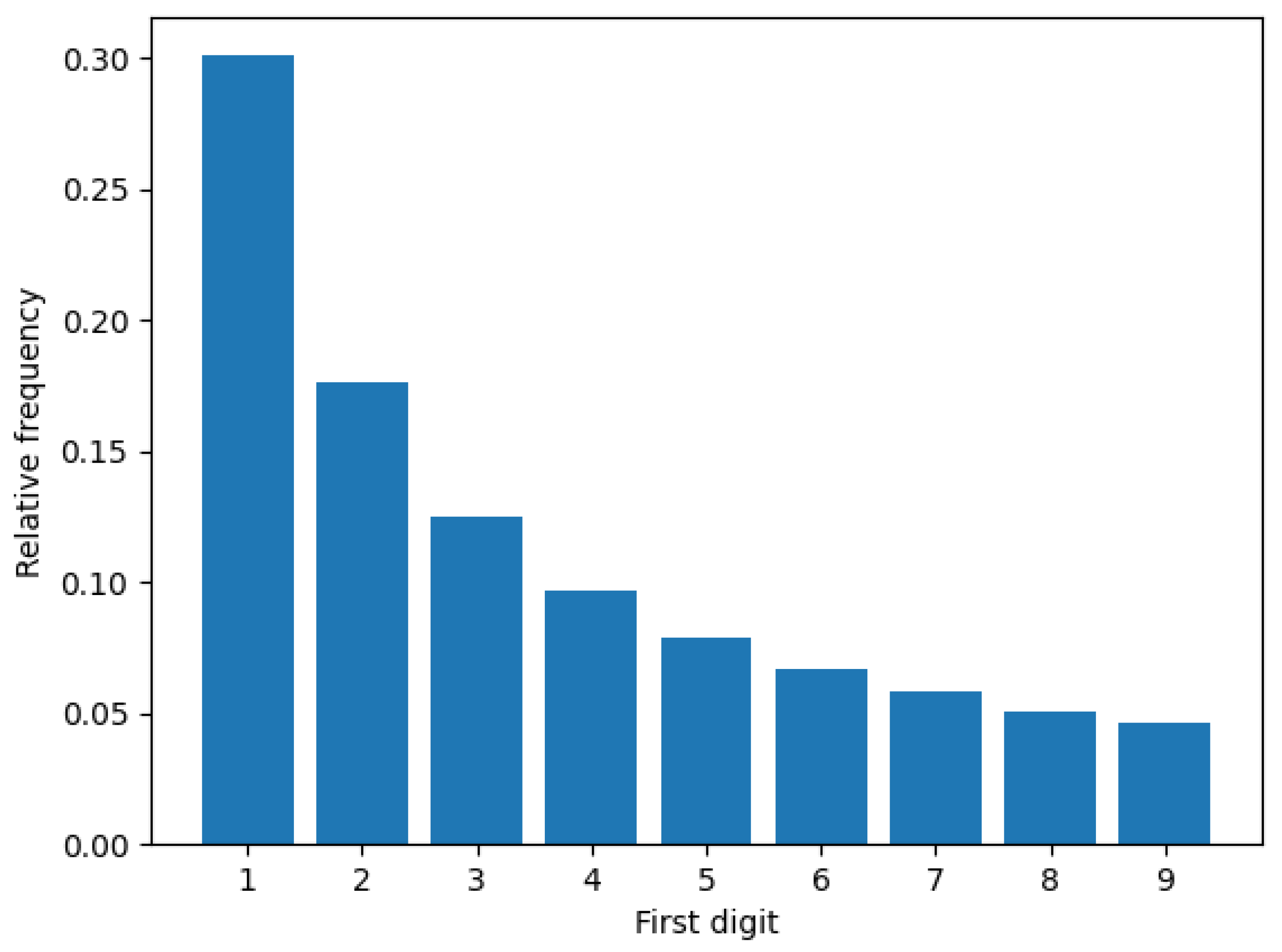
In this paper, we conduct thorough analysis on the features derived from Benford’s law for NR-IQA. Benford’s law, also known as the first digit law or the law of anomalous numbers, is an empirical observation about the relative frequency of first digits in many natural datasets. It was named after Frank Benford who was a physicist at the General Electric Research Laboratories in New York. He noticed that the first few pages of log tables were more worn than the last few pages. As a consequence, the front of the book was more used than the back of the book because there were more numbers that started with low digits than those of started with high digits. According to Benford’s law, the first digit d ( d { 1 , . . . , 9 } ) occurs with probability
P ( d ) = log 10 ( d + 1 ) log 10 ( d ) = log 10 d + 1 d = log 10 1 + 1 d .
The distribution of Benford’s law prediction (Equation (1)) is depicted in Figure 1. Benford’s law has been observed in many natural datasets, such as population numbers, length of rivers, mathematical and physical constants, etc., [13]. In image processing, Jolion [14] was the first who demonstrated that gradient images obey the Benford’s law, although it is not satisfied in the pixel domain, as pixel values distribute between 0 and 255. Similarly, Pérez-González et al. [15] pointed out that the discrete cosine transform (DCT) coefficients of an image follow the distribution predicted by Benford’s law.
First, Li [16] proposed a Benford’s law based metric combined with color ingredient, image complexity, image order, and Machado–Cardoso metric [17] to establish an aesthetic-aware feature vector. Specifically, the Benford’s law-based metric was determined as the distance between the first digit distribution (FDD) of Benford’s law prediction and those of 9 bins lightness histogram. A similar approach was taken by Ou et al. [18] in NR-IQA. A composite feature vector of 51-dimension was proposed where two elements were derived with the help of Benford’s law. Specifically, the Euclidean distance between the FDD of the input image’s DCT coefficients and the FDD predicted by Benford’s law was taken first. Subsequently, one more feature was extracted with the difference that the image is processed first with a Gaussian low pass filter. In our previous work [19], FDD in the wavelet domain was defined as a quality aware feature vector and used it as a part of a larger composite feature vector for NR-IQA.
The contributions of this work are summarized as follows.
  • We analyze the FDD-based features in different domains (wavelet, DCT, Shearlet, etc.) for NR-IQA. Unlike in our previous work [19], we focus on quality-aware feature vectors derived from FDD distributions of different domains.
  • We apply various regression methods including support vector regression (SVR), Gaussian process regression (GPR), binary tree regression (BTR), and random forest regression (RFR) to give a through performance analysis.
  • We conduct comparative analysis with other state-of-the-art methods on a wide range of publicly available IQA databases containing natural images with authentic and artificial distortions, screen-content images, and synthetic digital images.

Structure of the Paper

The paper is organized as follows. The related work is surveyed in Section 2. In Section 3, our method for FDD feature vector compilation is described. Section 4 presents the experimental results with analysis. Finally, a conclusion is drawn in Section 5.

2. Related Work

As already mentioned, the goal of NR-IQA is to predict the perceptual quality of digital images without any information about their distortion-free, reference counterpart. In the literature, NR-IQA algorithms are tested on publicly available benchmark image quality assessment databases, such as CLIVE [20], KonIQ-10k [21], or SPAQ [22], where digital images with their mean opinion score (MOS) or differential mean opinion score (DMOS) values are available. Specifically, individual quality scores are collected from human users for each distorted image either in a laboratory environment [23] or in a crowdsourcing-based experiment [10]. Moreover, MOS is determined as an arithemtic mean of individual scores, while DMOS is calculated as the difference between the raw quality score of the reference and test images [24]. An overview about subjective image quality assessment and publicly available benchmark databases can be found in the book of Xu et al. [25].
NR-IQA algorithms can be grouped into two classes: distortion-specific and general purpose. As the name indicates, distortion-specific NR-IQA algorithms are designed for specific distortion types, such as JPEG [26] or JPEG2000 [27] compression noise. In contrast, general purpose NR-IQA methods are designed to perform over different distortion types. The approach of natural scene statistics (NSS) has been very popular in general purpose NR-IQA. Namely, natural images exhibit a number of statistical regularities in spatial and transform domains that have been utilized to compile feature vectors for perceptual image quality prediction. For instance, blind image quality index (BIQI) decomposes first a distorted image over three scales and orientations using wavelet transform. Subsequently, generalized Gaussian distributions (GGD) are fitted to the wavelet coefficients and 18 quality-aware features are extracted. Finally, the features are mapped onto perceptual quality scores using a trained SVR. Another example is Distortion Identification-based Image Verity and INtegrity Evaluation (DIIVINE) [28] method where a GGD is fitted to the wavelet coefficients of a distorted image. The parameters of the obtained GGD were utilized as quality-aware feature and mapped onto quality scores with the help of a trained SVR. In contrast, Saad et al. [29] first divided the distorted image into blocks and a GGD is fitted onto the discrete cosine transform (DCT) coefficients of each block. The parameters of the GGDs are pooled from each block to create a feature vector. Finally, this feature vector is mapped onto quality scores with an SVR. Zhang et al. [30] proposed an improved NSS model where the errors of GGD parameter fitting were taking into account during the feature extraction step.
Recently, data-driven approaches have gained popularity in NR-IQA that do not rely on NSS-based or other hand-crafted features [31,32]. The work of Lv et al. [33] is a transition between hand-crafted features based and deep learning based approaches. Namely, the authors capitalized on the multi-scale difference of Gaussian (DoG) to decompose the distorted image in the spatial domain to extract quality-aware features. Next, a three-layer stacked autoencoder was used for the generation of feature representations and an SVR was utilized for perceptual quality prediction. In contrast, Kang et al. [34] trained a convolutional neural network (CNN) on image patches from scratch to estimate image quality. Similarly, Li et al. [35] trained a CNN on image patches but it was combined with the Prewitt magnitude of segmented images to obtain perceptual quality scores. In contrast, Ma et al. [36] introduced a multi-task CNN to improve the performance of image quality prediction with image distortion identification. The above-mentioned CNN-based NR-IQA approaches consider the input image’s perceptual quality as the arithmetic mean of the image patches’ predicted quality. He et al. [37] elaborated a pooling strategy where the image patches’ importance depend on their visual saliency. Tang et al. [38] trained and fine-tuned a deep belief network to estimate perceptual image quality. Kim and Lee [39] first trained a CNN on a large number of image patches acquiring quality scores with the help of a traditional FR-IQA metric.
Comprehensive overviews about IQA or NR-IQA can be found in [9,25,40,41].

3. Methods

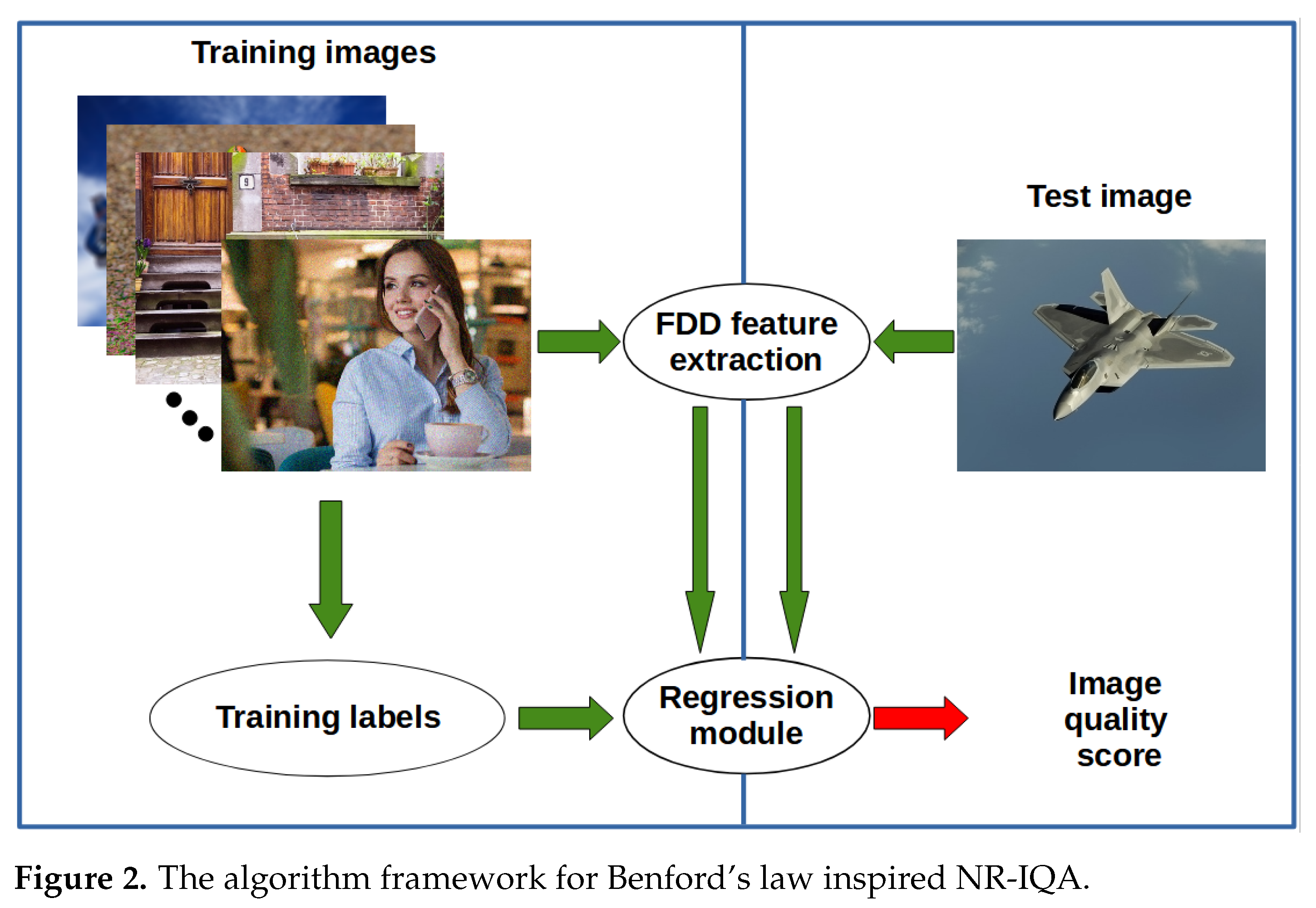
Figure 2 depicts the algorithmic framework of the test environment for Benford’s law inspired no-reference image quality assessment. Specifically, the framework can be divided into two phases. First, the extracted FDD feature vectors and the ground-truth quality scores of the training images are sent to the regression module. Second, the extracted FDD features of a test image are sent to the trained regression module to predict its perceptual quality score. In [19], it was pointed out that the FDD in different transform domains matches very well with Benford’s law in case of high quality images. Table 1 illustrates the mean FDD of singular values in KADID-10k with respect to the five distortion levels found in this database. On the other hand, Table 2 depicts the mean FDD of DCT coefficients with respect to five equal MOS intervals in KonIQ-10k [21] database. It can be observed that the distance between the actual FDD and Benford’s law prediction is roughly proportional to the level of distortion. In these tables, the distance between distributions is characterized by the symmetric Kullback–Leibler ( s K L ) divergence which is defined as between distributions P ( x ) and B ( x ) :
s K L ( P ( x ) , B ( x ) ) = 1 2 K L ( P ( x ) , B ( x ) ) + 1 2 K L ( B ( x ) , P ( x ) ) ,
where the Kullback–Leibler (KL) divergence is given as
K L ( P ( x ) , B ( x ) ) = i = 1 n P ( x ) log 2 P ( x ) B ( x ) .
In this paper, we analyze the efficiency of FDD in horizontal wavelet coefficients, vertical wavelet coefficients, diagonal wavelet coefficients, DCT coefficients, singular values, and the absolute values of shearlet coefficients for image quality prediction without reference images.
Wavelet transforms were devised to overcome the limitations of the Fourier transform. Namely, the Fourier transform decomposes signals into sine and cosine waves of specific frequencies. In contrast, the wavelet transform decomposes signals into shifted and scaled versions of a wavelet. Moreover, a function’s average has to be equal to zero to be a wavelet. In this study, we take the single-level 2D discrete wavelet transform of a digital image applying the order 4 symlet and periodic extension. Moreover, we obtain the FDD from the horizontal, vertical, and diagonal coefficients of the input image’s wavelet transform.
DCT describes digital images as sums of sinusoids of varying amplitudes and frequencies. It is often applied in image compression, as significant information about the image can be found in a few DCT coefficients [43]. The DCT of a M × N grayscale image I is defined as follows:
B p q = α p α q m = 0 M 1 n = 0 N 1 I m n cos π ( 2 m + 1 ) p 2 M cos π ( 2 n + 1 ) q 2 N , 0 p M 1 , 0 q N 1 ,
α p = 1 M , p = 0 2 M , 1 p M 1 ,
α q = 1 N , q = 0 2 N , 1 q N 1 ,
where B p q values are the DCT coefficients of image I.
Singular value decomposition (SVD) can be described as an algorithm for data reduction, as it identifies and orders the dimensions along which data points show the most variation. SVD decomposed a matrix into three other matrices:
A = U S V T ,
where A is an m × n matrix, U is an m × n orthogonal matrix, S is an n × n diagonal matrix, and V is an n × n orthogonal matrix. Moreover, S contains the square roots of eigenvalues from U or V in descending order.
The shearlet transform is a multi-scale extension of the traditional wavelet transform so that can handle anisotropic and directional information at multiple scales [44]. The parabolic scale matrix ( A c , c R + ) and the shear matrix ( S b , b R ) are required to define a Shearlet system. Formally, they can be expressed as
A c = c 0 0 c ,
S b = 1 b 0 1 .
Subsequently, the shearlet system can be given as
{ ψ g , h , m ( x ) : = 2 3 2 g ψ ( S h A 4 g x m ) : g , h Z , m Z 2 } ,
where g is the scale parameter, h is the angle parameter, and m is the position parameter. If these parameters are discretized, a discrete shearlet system can be obtained. The discrete shearlet transform of function f L 2 ( R 2 ) corresponds to the inner product of f with all the shearlets that can be found in the discrete shearlet system.
In this study, the effects of extended FDD feature vectors for NR-IQA are also investigated. The extended FDD feature vectors augment FDD feature vectors by adding certain divergence and shape parameters to the original FDD. After obtaining the FDD feature vector of an image, the s K L divergence between the actual FDD and Benford’s law prediction, the skewness, the kurtosis, the entropy, the median, and the standard deviation of the actual FDD were attached to the FDD feature vector to obtain the extended FDD feature vector. As a result, the length of the extended FDD is 15.

4. Experimental Results and Analysis

In this section, our experimental results and analysis are presented. Specifically, a general overview about the used IQA databases is given in Section 4.1.

4.1. Databases

In this section, an overview is given about the applied publicly available IQA databases.
In the past decade, an increasing number of publicly available IQA databases containing natural, screen-content, or synthetic images have been released for research [21]. The images found in IQA databases have been evaluated in subjective user studies involving human subjects in a laboratory environment [11] or crowdsourcing experiment [10] to obtain individual quality ratings. These IQA databases can be divided into two groups with respect to the type of image distortions (artificial or authentic). The first group contains a small set of reference, pristine, distortion-free images and a large set of distorted images derived from the reference images using various artificial distortions (Gaussian blur, motion blur, contrast change, etc.) at different levels. In contrast, the images of the second group were collected from public multimedia databases or personal collections. Therefore, they contain authentic distortions.
Table 3. Publicly available IQA benchmark databases used in this paper.
Database#Reference Images#Distorted ImagesResolutionEnvironment
TID2013 [45]243000 512 × 384 laboratory
CLIVE [20]-1162 500 × 500 crowdsourcing
KonIQ-10k [21]-10,073 1024 × 768 crowdsourcing
KADID-10k [42]8111,125 512 × 384 laboratory
SIQAD [46]20980 1280 × 720 laboratory
SCID [47]401800 672 × 682 laboratory
ESPL v2.0 [48]25500 1920 × 1080 laboratory
The TID2013 [45] IQA database contains 25 reference, pristine, distortion-free digital images. Distorted images were obtained from the reference images using 24 different distortion types in 5 different distortion levels. As a result, 3000 (= 25 × 24 × 5 ) distorted images can be found in this database. The images’ resolution is 512 × 384 .
The LIVE In the Wild Image Quality Challenge Database (CLIVE) [20] contains 1169 digital images with authentic distortions which were captured by different mobile camera devices. The images were evaluated in a crowdsourcing experiment by obtaining 350,000 opinion scores from 8100 unique human observers.
The KonIQ-10k [21] IQA database consists of 10,073 digital images with authentic distortions which were selected from the YFCC100m [49] public multimedia database. The images were evaluated by 1459 crowd workers. Moreover, MOS for each image was calculated from approximately 120 scores. The resolution of KonIQ-10k images is 1024 × 768 .
The KADID-10k [42] IQA database contains 81 reference, pristine, distortion-free digital images. Distorted images were created from the reference images applying 25 different distortion types in 5 different distortion levels.
Due to the continuous development of multimedia devices and displays, and the popularity of computer-generated imagery, screen content and synthetic images have received increasingly more attention in the image processing community [50,51,52]. In this paper, we consider two IQA databases with screen content images (SIQAD [46] and SCID [47]) and one IQA database with synthetic images (ESPL v2.0 [48]). Specifically, the SIQAD database consists of 20 reference and 980 distorted screen content images which were evaluated using the single stimulus methodology.
The SCID [47] database contains 40 reference screen content images. Moreover, 1800 distorted screen content images were generated from the reference images using 9 different distortion types at 5 different distortion levels. Each of the distorted images was evaluated at least by 40 human observers applying the double-stimulus impairment scale method.
The ESPL [48] database consists of synthetic images ( 1920 × 1080 pixels) chosen from video games and animation movies with corresponding quality scores. More specifically, it contains 25 synthetic reference images and 500 distorted synthetic images generated from the reference images using 5 different distortion types (interpolation, Gaussian blur, Gaussian noise, JPEG compression, fast fading channel) at 4 different distortion levels.
Table 3 summarizes the main characteristics of publicly available IQA databases used in this study.

4.2. Evaluation Metrics

In this subsection, the evaluation metrics of NR-IQA algorithms are presented. The performance evaluation and ranking of NR-IQA algorithms are based on the correlation between the predicted and ground-truth quality scores.
In the literature, Pearson’s linear correlation coefficient (PLCC), Spearman’s rank-order correlation coefficient (SROCC), and Kendall’s rank-order correlation coefficient are the most acknowledged performance measures which are reported in the majority of research papers [53]. Sheikh et al. [54] proposed applying a nonlinear mapping before the computation of PLCC,
q = β 1 0.5 1 1 + exp ( β 2 ( q β 3 ) ) + β 4 q + β 5 ,
where q and q stand for the objective quality scores after and before the mapping, respectively. In the literature, the q values are considered for PLCC computation. Let x and y vectors denote the vectors containing ground-truth and predicted quality scores of m images. Then, PLCC between x and y can be expressed as
P L C C ( x , y ) = i = 1 m ( x i x ¯ ) ( y i y ¯ ) i = 1 m ( x i x ¯ ) 2 i = 1 m ( y i y ¯ ) 2 ,
where
x ¯ = 1 m i = 1 m x i ,
and
y ¯ = 1 m i = 1 m y i .
SROCC between x and y can be calculated as
S R O C C ( x , y ) = i = 1 m ( x i x ) ( y i y ) i = 1 m ( x i x ) 2 i = 1 m ( y i y ) 2 ,
where x and y stand for the middle ranks of x and y , respectively. KROCC between x and y can be expressed as
K R O C C ( x , y ) = C D 1 2 m ( m 1 ) ,
where C stands for the number of pairs that correlates consistently between x and y , while D denotes the number of the other pairs.
In this study, we report on median PLCC, SROCC, and KROCC values measured over 1000 random train–test splits. Specifically, IQA databases containing authentic distortions (CLIVE [20] and KonIQ-10k [21]) were split randomly into training (approximately 80% of images) and test (approximately 20% of images) sets 1000 times and the median of the measured PLCC, SROCC, and KROCC values are reported. On the other hand, IQA databases with artificial distortions (TID2013 [45], KADID-10k [42], SIQAD [46], SCID [47], ESPL v2.0 [48]) were split randomly into training and test sets with respect to the reference images to avoid any semantic content overlap between these sets. Specifically, approximately 80% of reference images were selected and those distorted images which were derived from these reference images of the IQA database were used as a training set and the remaining distorted images were applied as a test set.

4.3. Evaluation Environment

The computer configuration applied in our experiments are summarized in Table 4. The proposed method was implemented and tested in MATLAB R2021a relying on the built-in functions of the Statistics and Machine Learning Toolbox, Image Processing Toolbox, and Wavelet Toolbox.

4.4. Parameter Study

In this subsection, a parameter study is presented which contains a detailed analysis about the different FDD feature vectors. Specifically, we examine the performance effects of FDD feature vectors extracted from horizontal, vertical, and diagonal wavelet coefficients, DCT coefficients, singular values, and shearlet coefficients. Moreover, we made experiments with five different regression algorithms, such as linear SVR, RBF-SVR, GPR with rational quadratic kernel function, binary regression tree (BTR), and random forest regression (RFR), to find the best performing method. The results obtained on KonIQ-10k [21], KADID-10k [42], SCID [47], and ESPL v2.0 [48] are summarized in Table 5, Table 6, Table 7 and Table 8. From these results, it can be clearly seen that GPR with rational quadratic kernel function is the best performing regression module. It outperforms all the other types of regression modules in all cases. The performance of individual FDD feature vectors is rather weak, but the concatenation of all types of FDDs exhibit a strong correlation with perceptual quality scores. Interestingly, ranking between different types of FDDs cannot be plainly established. On the one hand, FDD of Shearlet coefficients show the weakest correlation with perceptual quality scores in almost all cases. On the other hand, FDD of singular values exhibit a rather strong correlation with the quality scores of synthetic images (see Table 8 for the results of ESPL v2.0 [48]) but it gives the second weakest performance on screen content images (Table 7). For natural images with authentic distortions (Table 5), FDD of DCT coefficients provides the best and FDD of diagonal wavelet coefficients the second best results. However, the case is exactly the opposite for natural images with artificial distortions.

4.5. Comparison to the State-of-the-Art

Based on the results of the previous subsection, we propose four NR-IQA methods utilizing FFD feature vectors.
  • FDD-IQA: Its feature vectors contains the FDD of horizontal, vertical, and diagonal wavelet coefficients, DCT coefficients, singular values, and absolute values of Shearlet coefficients. As a result, the length of the feature vector is 9 × 6 = 54 .
  • FDD+Perceptual-IQA: Besides the features of FDD-IQA, it contains five perceptual features, such as colorfulness [55], global contrast factor [56], dark channel feature [57], entropy, and mean of the phase congruency image [58], which are considered consistent with human quality judgments in the literature [59]. As a result, the length of the feature vector is 9 × 6 + 5 = 59 .
  • eFDD-IQA: Its feature vectors contains the extended FDD of horizontal, vertical, and diagonal wavelet coefficients; DCT coefficients; singular values; and absolute values of Shearlet coefficients. As a result, the length of the feature vector is ( 9 + 6 ) × 6 = 90 .
  • eFDD+Perceptual-IQA: Besides the features of eFDD-IQA, it contains five perceptual features (colorfulness [55], global contrast factor [56], dark channel feature [57], entropy, mean of the phase congruency image [58]). As a result, the length of the feature vector is ( 9 + 6 ) × 6 + 5 = 95 .
All of the above-mentioned methods apply GPR with quadratic rational kernel function to map the extracted feature vectors onto perceptual quality scores, because it proved the best solution in the light of experimental results presented in the previous subsection.
The proposed four NR-IQA algorithms were compared on CLIVE [20], KonIQ-10k [21], TID2013 [45], KADID-10k [42], SCID [47], SIQAD [46], and ESPL v2.0 [48] to several state-of-the-art NR-IQA algorithms (BLIINDS-II [29], BMPRI [60], BRISQUE [61], CurveletQA [62], DIIVINE [28], ENIQA [63], GRAD-LOG-CP [64], NBIQA [18], OG-IQA [65], and SSEQ [66]) whose source codes were made publicly available by the authors. The evaluation metrics and protocol were exactly the same that were given in Section 4.2. The experimental results are summarized in Table 9, Table 10, Table 11 and Table 12. It can be observed from the presented results that it is possible to reach state-of-the-art performance relying only on FDD feature vectors. Moreover, FDDs augmented with perceptual features (colorfulness, global contrast factor, dark channel feature, entropy, mean of phase congruency image) are able to outperform the state-of-the-art on large IQA databases (KonIQ-10k [21] and KADID-10k [42]) with authentic and artificial distortions. The use of extended FDDs is able to improve the performance only on authentic distortions, screen-content images, and synthetic images. Furthermore, the popular perceptual features can improve the performance in the case of natural images both on authentic and artificial distortions. Surprisingly, FDD feature vectors are able to outperform the state-of-the-art on synthetic images by a large margin as one can see in Table 12. Table 13 summarizes the direct and weighted average PLCC, SROCC, and KROCC values computed from the results of the seven above mentioned IQA databases. It can be observed that FDD feature vectors augmented with perceptual features provide the second best results in the case of direct averages. On the other hand, FDD with perceptual features give the best results in the case of weighted averages. This indicates that the proposed method tends to perform better on larger databases, which can also be observed in Table 9, Table 10 and Table 11. Table 14 compares the computational times of the feature extractions of the proposed and other state-of-the-art methods using the computer configuration described in Table 4. It can be observed that the FDD feature extraction is rather fast on IQA databases with smaller resolution (CLIVE [20], TID2013 [45], and KADID-10k [42]). However, the computational times of FDD feature extraction grows rapidly with the image resolution. The reason for this can be derived from Table 15 and Table 16, where the profile summaries of FDD-IQA and FDD+Perceptual-IQA measured on KonIQ-10k [21] are presented. It can be seen that the shearlet transform and the computation of FDDs are responsible for ~98% of the computational time in the case of FDD-IQA. As the input image resolution increase, the number of wavelet, DCT, and shearlet coefficients increases and the computational time of FDDs in different domains increases in line with the number of the coefficients. Future work involves an effective implementation of feature extraction by carrying out Shearlet transform on GPU [67] and determining FDDs either by parallel programming or GPU computations.

5. Conclusions

In this paper, Benford’s law, also known as the first digit law, inspired feature vectors were proposed and studied for NR-IQA. Specifically, we analyzed FDD-based feature vectors extracted from different domains (wavelet, DCT, shearlet, singular values) for no-reference quality assessment of natural images with authentic or artificial distortions, screen-content images, and synthetic images. First, a detailed parameter study was presented with respect to different domains and different regression modules. Second, we demonstrated that state-of-the-art performance can be achieved by considering FDDs from different domains. Experimental results have been presented on various IQA benchmark databases containing natural, screen-content, and synthetic digital images.

Funding

This research received no external funding.

Institutional Review Board Statement

Not applicable.

Informed Consent Statement

Not applicable.

Data Availability Statement

The used datasets were obtained from publically open source datasets from: 1. CLIVE: https://live.ece.utexas.edu/research/ChallengeDB/index.html, (accessed on 23 September 2021) 2. KonIQ-10k: http://database.mmsp-kn.de/koniq-10k-database.html, (accessed on 23 September 2021) 3. TID2013: http://www.ponomarenko.info/tid2013.htm, (accessed on 23 September 2021) 4. KADID-10k: http://database.mmsp-kn.de/kadid-10k-database.html, (accessed on 23 September 2021) 5. SCID: http://smartviplab.org/pubilcations/SCID.html, (accessed on 23 September 2021) 6. SIQAD: https://sites.google.com/site/subjectiveqa/, (accessed on 23 September 2021) 7. ESPL v2.0: http://signal.ece.utexas.edu/~bevans/synthetic/ (accessed on 23 September 2021).

Acknowledgments

We thank the anonymous reviewers for their careful reading of our manuscript and their many insightful comments and suggestions.

Conflicts of Interest

The authors declare no conflict of interest.

Abbreviations

The following abbreviations are used in this manuscript:
BTRbinary tree regression
CNNconvolutional neural network
CPUcentral processing unit
DCTdiscrete cosine transform
DIIVINEDistortion Identification-based Image Verity and Integrity Evaluation
DMOSdifferential mean opinion score
DoGdifference of Gaussians
ESPLEmbedded Signal Processing Laboratory
FDDfirst digit distribution
FRfull-reference
GGDgeneralized Gaussian distribution
GPRGaussian process regression
GPUgraphics processing unit
IQAimage quality assessment
JPEGjoint photographic experts group
KLKullback–Leibler
KROCCKendall’s rank order correlation coefficient
LIVELaboratory for Image and Video Engineering
MOSmean opinion score
NRno-reference
NR-IQAno-reference image quality assessment
NSSnatural scene statistics
PLCCPearson’s linear correlation coefficient
RBFradial basis function
RFRrandom forest regressor
RRreduced-reference
SCIDscreen content image database
SIQADscreen image quality assessment database
sKLsymmetric Kullback–Leibler
SROCCSpearman’s rank order correlation coefficient
SVDsingular value decomposition
SVRsupport vector regressor
TIDTampere image database

References

  1. Chiasserini, C.F.; Magli, E. Energy consumption and image quality in wireless video-surveillance networks. In Proceedings of the 13th IEEE International Symposium on Personal, Indoor and Mobile Radio Communications, Lisbon, Portugal, 18 September 2002; Volume 5, pp. 2357–2361. [Google Scholar]
  2. Stępień, I.; Obuchowicz, R.; Piórkowski, A.; Oszust, M. Fusion of Deep Convolutional Neural Networks for No-Reference Magnetic Resonance Image Quality Assessment. Sensors 2021, 21, 1043. [Google Scholar] [CrossRef] [PubMed]
  3. Kalwa, J.; Madsen, A. Sonar image quality assessment for an autonomous underwater vehicle. In Proceedings of the World Automation Congress, Seville, Spain, 28 June–1 July 2004; Volume 15, pp. 33–38. [Google Scholar]
  4. Yurtsever, E.; Lambert, J.; Carballo, A.; Takeda, K. A survey of autonomous driving: Common practices and emerging technologies. IEEE Access 2020, 8, 58443–58469. [Google Scholar] [CrossRef]
  5. Chen, C.C.; Wan, Y.L.; Wai, Y.Y.; Liu, H.L. Quality assurance of clinical MRI scanners using ACR MRI phantom: Preliminary results. J. Digit. Imaging 2004, 17, 279–284. [Google Scholar] [CrossRef] [PubMed] [Green Version]
  6. Sdiri, B.; Kaaniche, M.; Cheikh, F.A.; Beghdadi, A.; Elle, O.J. Efficient enhancement of stereo endoscopic images based on joint wavelet decomposition and binocular combination. IEEE Trans. Med. Imaging 2018, 38, 33–45. [Google Scholar] [CrossRef]
  7. Tong, H.; Li, M.; Zhang, H.J.; Zhang, C.; He, J.; Ma, W.Y. Learning no-reference quality metric by examples. In Proceedings of the 11th International Multimedia Modelling Conference, Melbourne, VIC, Australia, 12–14 January 2005; pp. 247–254. [Google Scholar]
  8. Keelan, B. Handbook of Image Quality: Characterization and Prediction; CRC Press: Boca Raton, FL, USA, 2002. [Google Scholar]
  9. Wang, Z.; Bovik, A.C. Modern image quality assessment. Synth. Lect. Image Video Multimed. Process. 2006, 2, 1–156. [Google Scholar] [CrossRef] [Green Version]
  10. Saupe, D.; Hahn, F.; Hosu, V.; Zingman, I.; Rana, M.; Li, S. Crowd workers proven useful: A comparative study of subjective video quality assessment. In Proceedings of the QoMEX 2016: 8th International Conference on Quality of Multimedia Experience, Lisbon, Portugal, 6–8 June 2016. [Google Scholar]
  11. Zhang, H.; Li, D.; Yu, Y.; Guo, N. Subjective and Objective Quality Assessments of Display Products. Entropy 2021, 23, 814. [Google Scholar] [CrossRef]
  12. Winkler, S. Analysis of public image and video databases for quality assessment. IEEE J. Sel. Top. Signal Process. 2012, 6, 616–625. [Google Scholar] [CrossRef]
  13. Raimi, R.A. The first digit problem. Am. Math. Mon. 1976, 83, 521–538. [Google Scholar] [CrossRef]
  14. Jolion, J.M. Images and Benford’s law. J. Math. Imaging Vis. 2001, 14, 73–81. [Google Scholar] [CrossRef]
  15. Pérez-González, F.; Heileman, G.L.; Abdallah, C.T. Benford’s lawin image processing. In Proceedings of the 2007 IEEE International Conference on Image Processing, San Antonio, TX, USA, 16 September–19 October 2007; Volume 1, pp. I-405–I-408. [Google Scholar]
  16. Li, Y. Adaptive learning evaluation model for evolutionary art. In Proceedings of the 2012 IEEE Congress on Evolutionary Computation, Brisbane, QLD, Australia, 10–15 June 2012; pp. 1–8. [Google Scholar]
  17. Machado, P.; Cardoso, A. Computing aesthetics. In Brazilian Symposium on Artificial Intelligence; Springer: Berlin/Heidelberg, Germany, 1998; pp. 219–228. [Google Scholar]
  18. Ou, F.Z.; Wang, Y.G.; Zhu, G. A novel blind image quality assessment method based on refined natural scene statistics. In Proceedings of the 2019 IEEE International Conference on Image Processing (ICIP), Taipei, Taiwan, 22–25 September 2019; pp. 1004–1008. [Google Scholar]
  19. Varga, D. No-reference image quality assessment based on the fusion of statistical and perceptual features. J. Imaging 2020, 6, 75. [Google Scholar] [CrossRef]
  20. Ghadiyaram, D.; Bovik, A.C. Massive online crowdsourced study of subjective and objective picture quality. IEEE Trans. Image Process. 2015, 25, 372–387. [Google Scholar] [CrossRef] [Green Version]
  21. Lin, H.; Hosu, V.; Saupe, D. KonIQ-10K: Towards an ecologically valid and large-scale IQA database. arXiv 2018, arXiv:1803.08489. [Google Scholar]
  22. Fang, Y.; Zhu, H.; Zeng, Y.; Ma, K.; Wang, Z. Perceptual quality assessment of smartphone photography. In Proceedings of the IEEE/CVF Conference on Computer Vision and Pattern Recognition, Seattle, WA, USA, 13–19 June 2020; pp. 3677–3686. [Google Scholar]
  23. ITU-T Recommendation P. Subjective Video Quality Assessment Methods for Multimedia Applications; International Telecommunication Union: Geneva, Switzerland, 1999. [Google Scholar]
  24. Mohammadi, P.; Ebrahimi-Moghadam, A.; Shirani, S. Subjective and objective quality assessment of image: A survey. arXiv 2014, arXiv:1406.7799. [Google Scholar]
  25. Xu, L.; Lin, W.; Kuo, C.C.J. Visual Quality Assessment by Machine Learning; Springer: Berlin/Heidelberg, Germany, 2015. [Google Scholar]
  26. Zhan, Y.; Zhang, R. No-reference JPEG image quality assessment based on blockiness and luminance change. IEEE Signal Process. Lett. 2017, 24, 760–764. [Google Scholar] [CrossRef]
  27. Sazzad, Z.P.; Kawayoke, Y.; Horita, Y. No reference image quality assessment for JPEG2000 based on spatial features. Signal Process. Image Commun. 2008, 23, 257–268. [Google Scholar] [CrossRef]
  28. Moorthy, A.K.; Bovik, A.C. Blind image quality assessment: From natural scene statistics to perceptual quality. IEEE Trans. Image Process. 2011, 20, 3350–3364. [Google Scholar] [CrossRef]
  29. Saad, M.A.; Bovik, A.C.; Charrier, C. Blind image quality assessment: A natural scene statistics approach in the DCT domain. IEEE Trans. Image Process. 2012, 21, 3339–3352. [Google Scholar] [CrossRef]
  30. Zhang, Y.; Wu, J.; Xie, X.; Li, L.; Shi, G. Blind image quality assessment with improved natural scene statistics model. Digit. Signal Process. 2016, 57, 56–65. [Google Scholar] [CrossRef]
  31. Ma, J.; Wu, J.; Li, L.; Dong, W.; Xie, X.; Shi, G.; Lin, W. Blind Image Quality Assessment with Active Inference. IEEE Trans. Image Process. 2021, 30, 3650–3663. [Google Scholar] [CrossRef]
  32. Sun, W.; Min, X.; Zhai, G.; Gu, K.; Duan, H.; Ma, S. MC360IQA: A multi-channel CNN for blind 360-degree image quality assessment. IEEE J. Sel. Top. Signal Process. 2019, 14, 64–77. [Google Scholar] [CrossRef]
  33. Lv, Y.; Jiang, G.; Yu, M.; Xu, H.; Shao, F.; Liu, S. Difference of Gaussian statistical features based blind image quality assessment: A deep learning approach. In Proceedings of the 2015 IEEE International Conference on Image Processing (ICIP), Quebec City, QC, Canada, 27–30 September 2015; pp. 2344–2348. [Google Scholar]
  34. Kang, L.; Ye, P.; Li, Y.; Doermann, D. Convolutional neural networks for no-reference image quality assessment. In Proceedings of the IEEE Conference on Computer Vision and Pattern Recognition, Columbus, OH, USA, 23–28 June 2014; pp. 1733–1740. [Google Scholar]
  35. Li, J.; Zou, L.; Yan, J.; Deng, D.; Qu, T.; Xie, G. No-reference image quality assessment using Prewitt magnitude based on convolutional neural networks. Signal Image Video Process. 2016, 10, 609–616. [Google Scholar] [CrossRef]
  36. Ma, K.; Liu, W.; Zhang, K.; Duanmu, Z.; Wang, Z.; Zuo, W. End-to-end blind image quality assessment using deep neural networks. IEEE Trans. Image Process. 2017, 27, 1202–1213. [Google Scholar] [CrossRef] [PubMed]
  37. He, L.; Zhong, Y.; Lu, W.; Gao, X. A visual residual perception optimized network for blind image quality assessment. IEEE Access 2019, 7, 176087–176098. [Google Scholar] [CrossRef]
  38. Tang, H.; Joshi, N.; Kapoor, A. Blind image quality assessment using semi-supervised rectifier networks. In Proceedings of the IEEE Conference on Computer Vision and Pattern Recognition, Columbus, OH, USA, 23–28 June 2014; pp. 2877–2884. [Google Scholar]
  39. Kim, J.; Lee, S. Fully deep blind image quality predictor. IEEE J. Sel. Top. Signal Process. 2016, 11, 206–220. [Google Scholar] [CrossRef]
  40. Lahoulou, A.; Viennet, E.; Bouridane, A.; Haddadi, M. A complete statistical evaluation of state-of-the-art image quality measures. In Proceedings of the International Workshop on Systems, Signal Processing and their Applications, WOSSPA, Tipaza, Algeria, 9–11 May 2011; pp. 219–222. [Google Scholar]
  41. Phillips, J.B.; Eliasson, H. Camera Image Quality Benchmarking; John Wiley & Sons: Hoboken, NJ, USA, 2018. [Google Scholar]
  42. Lin, H.; Hosu, V.; Saupe, D. KADID-10k: A large-scale artificially distorted IQA database. In Proceedings of the 2019 Eleventh International Conference on Quality of Multimedia Experience (QoMEX), Berlin, Germany, 5–7 June 2019; pp. 1–3. [Google Scholar]
  43. Britanak, V.; Yip, P.C.; Rao, K.R. Discrete Cosine and Sine Transforms: General Properties, Fast Algorithms and Integer Approximations; Elsevier: Amsterdam, The Netherlands, 2010. [Google Scholar]
  44. Easley, G.; Labate, D.; Lim, W.Q. Sparse directional image representations using the discrete shearlet transform. Appl. Comput. Harmon. Anal. 2008, 25, 25–46. [Google Scholar] [CrossRef] [Green Version]
  45. Ponomarenko, N.; Jin, L.; Ieremeiev, O.; Lukin, V.; Egiazarian, K.; Astola, J.; Vozel, B.; Chehdi, K.; Carli, M.; Battisti, F.; et al. Image database TID2013: Peculiarities, results and perspectives. Signal Process. Image Commun. 2015, 30, 57–77. [Google Scholar] [CrossRef] [Green Version]
  46. Yang, H.; Fang, Y.; Lin, W. Perceptual quality assessment of screen content images. IEEE Trans. Image Process. 2015, 24, 4408–4421. [Google Scholar] [CrossRef]
  47. Ni, Z.; Ma, L.; Zeng, H.; Fu, Y.; Xing, L.; Ma, K.K. SCID: A database for screen content images quality assessment. In Proceedings of the 2017 International Symposium on Intelligent Signal Processing and Communication Systems (ISPACS), Xiamen, China, 6–9 November 2017; pp. 774–779. [Google Scholar]
  48. Kundu, D.; Choi, L.K.; Bovik, A.C.; Evans, B.L. Perceptual quality evaluation of synthetic pictures distorted by compression and transmission. Signal Process. Image Commun. 2018, 61, 54–72. [Google Scholar] [CrossRef]
  49. Kalkowski, S.; Schulze, C.; Dengel, A.; Borth, D. Real-time analysis and visualization of the YFCC100M dataset. In Proceedings of the 2015 Workshop on Community-Organized Multimodal Mining: Opportunities for Novel Solutions, Brisbane, Australia, 30 October 2015; pp. 25–30. [Google Scholar]
  50. Ni, Z.; Ma, L.; Zeng, H.; Cai, C.; Ma, K.K. Screen content image quality assessment using edge model. In Proceedings of the 2016 IEEE International Conference on Image Processing (ICIP), Phoenix, AZ, USA, 25–28 September 2016; pp. 81–85. [Google Scholar]
  51. Ni, Z.; Ma, L.; Zeng, H.; Cai, C.; Ma, K.K. Gradient direction for screen content image quality assessment. IEEE Signal Process. Lett. 2016, 23, 1394–1398. [Google Scholar] [CrossRef]
  52. Yang, H.; Fang, Y.; Lin, W.; Wang, Z. Subjective quality assessment of screen content images. In Proceedings of the 2014 Sixth International Workshop on Quality of Multimedia Experience (QoMEX), Singapore, 18–20 September 2014; pp. 257–262. [Google Scholar]
  53. Ding, Y. Visual Quality Assessment for Natural and Medical Image; Springer: Berlin/Heidelberg, Germany, 2018. [Google Scholar]
  54. Sheikh, H.R.; Sabir, M.F.; Bovik, A.C. A statistical evaluation of recent full reference image quality assessment algorithms. IEEE Trans. Image Process. 2006, 15, 3440–3451. [Google Scholar] [CrossRef] [PubMed]
  55. Hasler, D.; Suesstrunk, S.E. Measuring colorfulness in natural images. In Human Vision and Electronic Imaging VIII; International Society for Optics and Photonics: Bellingham, WA, USA, 2003; Volume 5007, pp. 87–95. [Google Scholar]
  56. Matkovic, K.; Neumann, L.; Neumann, A.; Psik, T.; Purgathofer, W. Global contrast factor—A new approach to image contrast. In Computational Aesthetics in Graphics, Visualization and Imaging; Eurographics Association: Girona, Spain, 2005; pp. 159–168. [Google Scholar]
  57. He, K.; Sun, J.; Tang, X. Single image haze removal using dark channel prior. IEEE Trans. Pattern Anal. Mach. Intell. 2010, 33, 2341–2353. [Google Scholar]
  58. Kovesi, P. Phase congruency detects corners and edges. In Proceedings of the Australian Pattern Recognition Society Conference: DICTA, Sydney, Australia, 10–12 December 2003. [Google Scholar]
  59. Jenadeleh, M. Blind Image and Video Quality Assessment. Ph.D. Thesis, University of Konstanz, Konstanz, Germany, 2018. [Google Scholar]
  60. Min, X.; Zhai, G.; Gu, K.; Liu, Y.; Yang, X. Blind image quality estimation via distortion aggravation. IEEE Trans. Broadcast. 2018, 64, 508–517. [Google Scholar] [CrossRef]
  61. Mittal, A.; Moorthy, A.K.; Bovik, A.C. No-reference image quality assessment in the spatial domain. IEEE Trans. Image Process. 2012, 21, 4695–4708. [Google Scholar] [CrossRef] [PubMed]
  62. Liu, L.; Dong, H.; Huang, H.; Bovik, A.C. No-reference image quality assessment in curvelet domain. Signal Process. Image Commun. 2014, 29, 494–505. [Google Scholar] [CrossRef]
  63. Chen, X.; Zhang, Q.; Lin, M.; Yang, G.; He, C. No-reference color image quality assessment: From entropy to perceptual quality. EURASIP J. Image Video Process. 2019, 2019, 77. [Google Scholar] [CrossRef] [Green Version]
  64. Xue, W.; Mou, X.; Zhang, L.; Bovik, A.C.; Feng, X. Blind image quality assessment using joint statistics of gradient magnitude and Laplacian features. IEEE Trans. Image Process. 2014, 23, 4850–4862. [Google Scholar] [CrossRef]
  65. Liu, L.; Hua, Y.; Zhao, Q.; Huang, H.; Bovik, A.C. Blind image quality assessment by relative gradient statistics and adaboosting neural network. Signal Process. Image Commun. 2016, 40, 1–15. [Google Scholar] [CrossRef]
  66. Liu, L.; Liu, B.; Huang, H.; Bovik, A.C. No-reference image quality assessment based on spatial and spectral entropies. Signal Process. Image Commun. 2014, 29, 856–863. [Google Scholar] [CrossRef]
  67. Gibert, X.; Patel, V.M.; Labate, D.; Chellappa, R. Discrete shearlet transform on GPU with applications in anomaly detection and denoising. EURASIP J. Adv. Signal Process. 2014, 2014, 64. [Google Scholar] [CrossRef]
Figure 1. Distribution of first digits in natural datasets according to Benford’s law. Each bar represents a digit, and the height is proportional to the relative frequency of numbers that begin with that digit.
Electronics 10 02378 g001
Figure 2. The algorithm framework for Benford’s law inspired NR-IQA.
Electronics 10 02378 g002
Table 1. Mean FDD of singular values in KADID-10k with respect to reference images and five distinct distortion levels found in KADID-10k [42]. Level 1 corresponds to the lowest amount of distortion, while Level 5 stands for the highest amount. In the last column, the symmetric Kullback–Leibler ( s K L ) divergences between the actual FDD and Benford’s law distribution are given.
123456789 s K L
Reference0.3130.1850.1250.0930.0740.0620.0550.0490.0440.002
Level 10.3070.1840.1260.0950.0760.0640.0550.0490.044 8.52 × 10 4
Level 20.3060.1810.1240.0950.0770.0650.0570.0500.045 3.08 × 10 4
Level 30.3120.1820.1230.0920.0750.0640.0560.0500.046 8.59 × 10 4
Level 40.3170.1850.1240.0900.0720.0620.0550.0490.0450.002
Level 50.3150.1920.1280.0920.0710.0600.0530.0480.0440.004
Benford’s law0.3010.1760.1250.0970.0790.0670.0580.0510.0460
Table 2. Mean FDD of DCT coefficients in KonIQ-10k [21] with respect to different MOS intervals. In  KonIQ-10k [21], lowest possible image quality is represented by M O S = 1.0 , while M O S = 5.0 stands for the highest possible image quality. In the last column, the symmetric Kullback–Leibler ( s K L ) divergences between the actual FDD and Benford’s law distribution are given.
123456789 sKL
4.2 M O S 5 0.2890.1780.1310.1020.0820.0670.0570.0500.044 9.3 × 10 4
3.4 M O S < 4.2 0.3030.1770.1250.0960.0780.0660.0570.0510.046 4.3 × 10 5
2.6 M O S < 3.4 0.3100.1760.1220.0940.0770.0660.0580.0520.047 4.2 × 10 4
1.8 M O S < 2.6 0.3150.1720.1180.0920.0770.0660.0590.0530.0480.0012
1 M O S < 1.8 0.3140.1690.1170.0920.0780.0680.0600.0540.0490.0016
Benford’s law0.3010.1760.1250.0970.0790.0670.0580.0510.0460
Table 4. Computer configuration applied in our experiments.
Computer modelSTRIX Z270H Gaming
CPUIntel(R) Core(TM) i7-7700K CPU 4.20 GHz (8 cores)
Memory15 GB
GPUNvidia GeForce GTX 1080
Table 5. Comparison of different FDD feature vectors extracted from different domains and different regression modules on KonIQ-10k [21] database. Median SROCC values were measured over 1000 random train–test splits.
FDDLinear SVRRBF-SVRGPRBTRRFR
Wavelet horizontal coefficients0.2450.4660.4700.2630.315
Wavelet vertical coefficients0.2500.4790.4830.2750.326
Wavelet diagonal coefficients0.2170.4830.4860.2740.324
DCT coefficients0.3360.5210.5340.3340.334
Singular values0.1520.3560.3570.1790.246
Absolute Shearlet coefficients0.1350.4400.4460.2540.308
All0.4070.6550.6910.4710.555
Table 6. Comparison of different FDD feature vectors extracted from different domains and different regression modules on KADID-10k [42] database. Median SROCC values were measured over 1000 random train–test splits.
FDDLinear SVRRBF-SVRGPRBTRRFR
Wavelet horizontal coefficients0.2500.2870.3110.1810.201
Wavelet vertical coefficients0.2580.3150.3230.1960.226
Wavelet diagonal coefficients0.2910.3940.3960.2460.280
DCT coefficients0.1960.3440.3550.2060.242
Singular values0.1570.3040.3150.1810.234
Absolute Shearlet coefficients−0.0110.1660.1710.0750.091
All0.3680.6050.6070.4160.468
Table 7. Comparison of different FDD feature vectors extracted from different domains and different regression modules on SCID [47] database. Median SROCC values were measured over 1000 random train–test splits.
FDDLinear SVRRBF-SVRGPRBTRRFR
Wavelet horizontal coefficients0.1130.3070.2890.1820.181
Wavelet vertical coefficients0.1030.3210.3030.1970.206
Wavelet diagonal coefficients0.1400.3230.3170.2030.204
DCT coefficients0.4410.3980.4420.2710.260
Singular values0.2970.2690.2840.1890.168
Absolute Shearlet coefficients0.2240.2410.2790.1600.152
All0.4450.4610.4950.3050.331
Table 8. Comparison of different FDD feature vectors extracted from different domains and different regression modules on ESPL v2.0 [48] database. Median SROCC values were measured over 1000 random train–test splits.
FDDLinear SVRRBF-SVRGPRBTRRFR
Wavelet horizontal coefficients0.3210.5030.5630.3540.347
Wavelet vertical coefficients0.2260.4500.5350.3760.364
Wavelet diagonal coefficients0.2370.4380.5450.4070.400
DCT coefficients0.0010.4230.4490.3560.338
Singular values0.4240.5810.6060.4780.487
Absolute Shearlet coefficients0.2020.2910.3310.1440.159
All0.6670.6950.7740.5420.560
Table 9. Comparison of FDD-based NR-IQA methods to the state-of-the-art on authentic distortions (CLIVE [20] and KonIQ-10k [21]). Median PLCC, SROCC, and KROCC values were measured over 1000 random train–test splits. Best results are typed in bold, and second best results are underlined.
CLIVE [20]KonIQ-10k [21]
MethodPLCCSROCCKROCCPLCCSROCCKROCC
BLIINDS-II [29]0.4750.4330.3010.5650.5620.410
BMPRI [60]0.5380.4830.3330.6390.6200.436
BRISQUE [61]0.5200.4870.3320.7070.6760.483
CurveletQA [62]0.6320.6120.4330.7280.7150.520
DIIVINE [28]0.6200.5810.4050.7110.6910.497
ENIQA [63]0.5930.5560.3870.7590.7440.545
GRAD-LOG-CP [64]0.6000.5670.3980.7050.6960.501
NBIQA [18]0.6250.6000.4190.7710.7480.550
OG-IQA [65]0.5390.4960.3400.6530.6340.447
SSEQ [66]0.4790.4290.2950.5880.5730.402
FDD-IQA0.5120.4670.3220.7290.6910.498
FDD+Perceptual-IQA0.5690.5430.3780.7770.7480.551
eFDD-IQA0.5060.4720.3240.7250.6880.495
eFDD+Perceptual-IQA0.5640.5420.3770.7740.7420.546
Table 10. Comparison of FDD-based NR-IQA methods to the state-of-the-art on artificial distortions (TID2013 [45] and KADID-10k [42]). Median PLCC, SROCC, and KROCC values were measured over 1000 random train–test splits. Best results are typed in bold, and second best results are underlined.
TID2013 [45]KADID-10k [42]
MethodPLCCSROCCKROCCPLCCSROCCKROCC
BLIINDS-II [29]0.5240.4920.3440.5450.5250.376
BMPRI [60]0.7000.5900.4270.5570.5320.381
BRISQUE [61]0.5740.4210.2940.3890.3950.275
CurveletQA [62]0.5550.4640.3290.4760.4480.317
DIIVINE [28]0.5240.4920.3440.4300.4370.308
ENIQA [63]0.6020.5430.3900.6330.6350.462
GRAD-LOG-CP [64]0.4320.2790.1920.5840.5660.411
NBIQA [18]0.6920.6220.4530.6170.6100.442
OG-IQA [65]0.5770.4600.3250.3990.3310.230
SSEQ [66]0.6200.5240.3750.4570.4350.303
FDD-IQA0.6860.5840.4230.6630.6070.438
FDD+Perceptual-IQA0.6830.5880.4270.7330.6920.509
eFDD-IQA0.6850.5780.4180.6660.6130.443
eFDD+Perceptual-IQA0.6820.5850.4240.7240.6830.498
Table 11. Comparison of FDD-based NR-IQA methods to the state-of-the-art on screen content images (SCID [47] and SIQAD [46]). Median PLCC, SROCC, and KROCC values were measured over 1000 random train–test splits. Best results are typed in bold, and second best results are underlined.
SCID [47]SIQAD [46]
MethodPLCCSROCCKROCCPLCCSROCCKROCC
BLIINDS-II [29]0.5970.5730.4300.6880.6580.474
BMPRI [60]0.6510.6170.4420.7500.7050.516
BRISQUE [61]0.4390.4370.2980.6350.5420.372
CurveletQA [62]0.4950.4610.3230.6280.5490.382
DIIVINE [28]0.5780.5470.3850.6500.6160.431
ENIQA [63]0.6200.5880.4260.6940.6600.475
GRAD-LOG-CP [64]0.7110.7030.5110.7280.6940.503
NBIQA [18]0.6700.6560.4700.7690.7390.544
OG-IQA [65]0.3310.3170.2170.6960.6560.473
SSEQ [66]0.5340.5190.3610.7010.6590.473
FDD-IQA0.5210.4950.3450.6510.6200.441
FDD+Perceptual-IQA0.5190.4940.3430.6370.6140.441
eFDD-IQA0.5240.5000.3470.6560.6240.444
eFDD+Perceptual-IQA0.5230.5020.3480.6530.6250.447
Table 12. Comparison of FDD-based NR-IQA methods to the state-of-the-art on synthetic images (ESPL v2.0 [48]). Median PLCC, SROCC, and KROCC values were measured over 1000 random train–test splits. Best results are typed in bold, and second best results are underlined.
ESPL v2.0 [48]
MethodPLCCSROCCKROCC
BLIINDS-II [29]0.6300.6270.448
BMPRI [60]0.7210.7400.541
BRISQUE [61]0.5590.5730.404
CurveletQA [62]0.7150.7230.529
DIIVINE [28]0.6390.6650.477
ENIQA [63]0.6780.6840.495
GRAD-LOG-CP [64]0.7040.7150.511
NBIQA [18]0.7000.7010.514
OG-IQA [65]0.7210.7160.527
SSEQ [66]0.5610.5230.370
FDD-IQA0.7680.7740.592
FDD+Perceptual-IQA0.7520.7540.569
eFDD-IQA0.7660.7750.594
eFDD+Perceptual-IQA0.7500.7540.568
Table 13. Comparison of FDD-based NR-IQA methods to the state-of-the-art. Direct and weighted average of PLCC, SROCC, and KROCC values are reported. Best results are typed in bold, second best results are underlined.
Direct AverageWeighted Average
MethodPLCCSROCCKROCCPLCCSROCCKROCC
BLIINDS-II [29]0.5750.5530.3980.5590.5430.391
BMPRI [60]0.6510.6120.4390.6180.5840.417
BRISQUE [61]0.5460.5040.3510.5460.5140.362
CurveletQA [62]0.6040.5670.4050.5940.5620.402
DIIVINE [28]0.5930.5760.4070.5690.5570.395
ENIQA [63]0.6540.6300.4540.6770.6610.481
GRAD-LOG-CP [64]0.6380.6030.4320.6270.5970.430
NBIQA [18]0.6920.6680.4850.6920.6710.489
OG-IQA [65]0.5590.5160.3660.5350.4840.341
SSEQ [66]0.5630.5230.3680.5410.5110.359
FDD-IQA0.6470.6050.4370.6790.6280.453
FDD+Perceptual-IQA0.6670.6330.4600.7240.6840.501
eFDD-IQA0.6470.6070.4380.6790.6300.453
eFDD+Perceptual-IQA0.6670.6330.4580.7200.6790.495
Table 14. Comparison of feature extractions’ computational times (in seconds). Best results are typed in bold, and second best results are underlined.
MethodCLIVE [20]KonIQ-10k [21]TID2013 [45]/KADID-10k [42]SCID [47]SIQAD [46]ESPL v2.0 [48]
BLIINDS-II [29]15.2347.2511.9611.67.01129.23
BMPRI [60]0.290.780.240.860.521.92
BRISQUE [61]0.030.110.030.140.070.31
CurveletQA [62]0.651.750.491.931.084.94
DIIVINE [28]6.9918.795.2722.2112.4657.82
ENIQA [63]4.1913.003.2514.808.1732.98
GRAD-LOG-CP [64]0.030.100.030.130.070.29
NBIQA [18]6.3520.075.0424.7413.4754.19
OG-IQA [65]0.030.100.020.130.070.30
SSEQ [66]0.411.280.331.530.833.40
FDD-IQA2.1716.192.6318.858.1662.94
FDD+Perceptual-IQA4.6523.974.5627.9213.0683.45
eFDD-IQA2.1816.202.6519.018.2163.33
eFDD+Perceptual-IQA4.6623.984.5828.0813.1183.84
Table 15. Profile summary of FDD-IQA measured on KonIQ-10k [21]. It presents statistics about the overall execution and a representation of the time spent in different modules of FDD-IQA.
Operation% of Total Time
Wavelet transform0.73%
Discrete cosine transform0.26%
Singular value decomposition0.75%
Shearlet transform34.63%
Computation of FDDs63.62%
Other0.01%
All100.0%
Table 16. Profile summary of FDD+Perceptual-IQA measured on KonIQ-10k [21]. It presents statistics about the overall execution and a representation of the time spent in different modules of FDD+Perceptual-IQA.
Operation% of Total Time
Wavelet transform0.47%
Discrete cosine transform0.17%
Singular value decomposition0.49%
Shearlet transform22.50%
Computation of FDDs41.34%
Colorfulness0.08%
Global contrast factor25.21%
Dark channel feature8.78%
Entropy0.01%
Mean of phase congruency0.94%
Other0.01%
All100.0%
Publisher’s Note: MDPI stays neutral with regard to jurisdictional claims in published maps and institutional affiliations.

