Article

Improving Semi-Supervised Learning for Audio Classification with FixMatch

by
Sascha Grollmisch
1,2,* and
Estefanía Cano
3,*
1
Fraunhofer IDMT, Industrial Media Applications (IMA), 98693 Ilmenau, Germany
2
TU Ilmenau, Institute for Media Technology, 98693 Ilmenau, Germany
3
Songquito UG, 91052 Erlangen, Germany
*
Authors to whom correspondence should be addressed.
Electronics 2021, 10(15), 1807; https://doi.org/10.3390/electronics10151807
Submission received: 16 June 2021 / Revised: 19 July 2021 / Accepted: 21 July 2021 / Published: 28 July 2021
(This article belongs to the Special Issue Machine Learning Applied to Music/Audio Signal Processing)

Abstract

:
Including unlabeled data in the training process of neural networks using Semi-Supervised Learning (SSL) has shown impressive results in the image domain, where state-of-the-art results were obtained with only a fraction of the labeled data. The commonality between recent SSL methods is that they strongly rely on the augmentation of unannotated data. This is vastly unexplored for audio data. In this work, SSL using the state-of-the-art FixMatch approach is evaluated on three audio classification tasks, including music, industrial sounds, and acoustic scenes. The performance of FixMatch is compared to Convolutional Neural Networks (CNN) trained from scratch, Transfer Learning, and SSL using the Mean Teacher approach. Additionally, a simple yet effective approach for selecting suitable augmentation methods for FixMatch is introduced. FixMatch with the proposed modifications always outperformed Mean Teacher and the CNNs trained from scratch. For the industrial sounds and music datasets, the CNN baseline performance using the full dataset was reached with less than 5% of the initial training data, demonstrating the potential of recent SSL methods for audio data. Transfer Learning outperformed FixMatch only for the most challenging dataset from acoustic scene classification, showing that there is still room for improvement.

1. Introduction

Recent advances in deep learning have resulted in improved performance for many classification tasks. However, such improvements often come at the expense of large annotated datasets and increasingly larger models. While datasets with the required amount of annotated data to train these models are not always available, unlabeled data can often be easily obtained. In the field of Acoustic Scene Classification (ASC), for example, edge devices can easily record large quantities of data at low additional cost. The same holds true for Industrial Sound Analysis (ISA) applications, where acoustic quality control systems can record the observed production process for long periods of time. In the field of Music Information Retrieval (MIR), vast amounts of music recordings can easily be collected for a given classification task from existing music collections.
The process of including labeled and unlabeled examples into the training process is called Semi-Supervised Learning (SSL). In the field of image classification, many SSL algorithms have recently pushed the state of the art and nearly closed the performance gap to models trained fully supervised using all annotated data [1,2,3,4,5]. On image classification datasets such as CIFAR-10 [6] with 4000 annotated labels (400 per class), the so-called FixMatch (FM) approach [3] (95.7% accuracy) outperformed previous SSL methods such as Mean Teacher (MT) [7] (90.8%) and Pseudo-Label (PL) [8] (83.0%). The performance gap between FM and all other evaluated SSL methods was even larger when the amount of labeled data was further reduced. In that scenario, FM also outperformed the supervised model (79.7%) and other Transfer Learning (TL) baselines (87.9%) [9]. Cances et al. [10] evaluated the potential of SSL methods such as FM and MT for audio data on Sound Event Detection (SED) and Speech Command Recognition (SCR) datasets. In their experiments, FM outperformed MT and the supervised baseline using 10% of the initial training data. Furthermore, the fully supervised baseline results were reached on two of the three datasets.
Despite the performance gains reported by these SSL approaches in the computer vision domain, and recently for audio data from the fields of SED and SCR, no research has been conducted to date (to the best of our knowledge) on the application of FM to ISA, ASC, and MIR. Additionally, results on image data show that performance is highly dependent on the type of augmentation methods used. However, many image augmentation methods cannot easily be applied to audio data for several reasons: (a) color channels frequently used for image augmentation such as hue change are not available in audio data (even though multi-channel audio recordings may be treated as multi-color channels in some cases), (b) image translations in x and y direction result in a very different modification than audio translations (location vs. time/frequency modification), (c) some augmentation methods do not work on all types of audio representation due to their different dimensionality (waveform, magnitude spectrogram, Mel-spectrogram, etc.).
The main contribution of this work is a systematic analysis of SSL approaches on audio classification tasks from Industrial Sound Analysis (ISA), Acoustic Scene Classification (ASC), and Music Information Retrieval (MIR). To this end, we implement the FM algorithm with adjustments to fit audio data, and compare its performance with MT, TL, and the corresponding supervised baselines. The amount of labeled data is gradually reduced to show the effectiveness of FM when only few annotated examples are available (few/one-shot learning). We propose a novel method to select the augmentation techniques used during training, as this choice was shown to be critical in a previous study [3] as well as in our experiments. All experiments are conducted with the same processing pipeline to avoid possible pitfalls in SSL evaluation which might occur with differences in data loading/splitting/pre-processing between the evaluated methods [9].
In the following sections, we first describe related work on SSL, data augmentations techniques for audio, and TL using pre-trained models for learning from few labels. We then explain the datasets used, our proposed SSL system, and the experimental design of our study. Finally, we report the results of our experiments and summarize our findings.

2. Related Work

This section summarizes related work on SSL for image and audio data, data augmentation for audio, and finally work on Transfer Learning using pre-trained audio embeddings.

2.1. Semi-Supervised Learning

The main idea behind SSL is to include unlabeled data into the training process and take advantage of large unlabeled datasets that can add variety to the training to build more robust classifiers, similar to using larger labeled datasets. The biggest challenge of SSL is that there is no guarantee that introducing unlabeled data into the training process will improve performance, and in some cases, it might even turn out to be detrimental [3,10,11]. One possible reason for this performance drop is the so-called confirmation bias, where incorrect predictions on the unlabeled data are amplified as the model overfits on these mistakes [7,12]. To provide some context on SSL, we briefly describe the SSL techniques that are most relevant for this work. For a detailed overview of previous SSL techniques, we refer the reader to [11].
Current SSL methods for classification tasks can be clustered into two main approaches: consistency regularization and entropy minimization. Consistency regularization is built upon the idea that realistic perturbations of the input data should not change predictions of the model [13]. An example for this approach is the Mean Teacher (MT) technique [7], where two separate models with the same architecture are trained: a teacher and a student model. The weights of the teacher model are an exponential moving average of the weights of the student model in previous iterations. The weights of the student model are updated using a combined loss term. The first term of the loss is obtained with the categorical cross-entropy (CCE) loss from classifying the augmented labeled data. The second term of the loss is a consistency term for the unlabeled data. The teacher model outputs predictions on weakly augmented data. The student is then forced to predict the same label distribution on the non-augmented version of the data. Mean squared error showed the best performance for this consistency loss. The final loss is a weighted sum of the CCE and the consistency loss.
In contrast, models using entropy minimization are pushed to output more confident predictions for unlabeled data. A commonly used entropy minimization method is the Pseudo-Label (PL) approach, where a given model predicts labels for the unlabeled data [8]. The class with the highest probability is taken as the true label and treated like ground truth. The CCE loss of the labeled data is combined with the weighted CCE loss of the unlabeled data. The selection and scheduling of the weighting factor (e.g., slowly increasing it over time) for the unlabeled loss is critical to avoid noisy pseudo labels from disturbing the training.
MixMatch (MM) combines entropy minimization with consistency regularization and resulted in improved performance in image classification tasks [1]. In MM, unlabeled examples are augmented several times and the output distributions are averaged and used as the target. To encourage high confidence predictions, the entropy of the output distribution is minimized by emphasizing the highest confidence prediction and lowering the others accordingly in a process called “sharpening”. For further details on the “sharpening” process, we refer the reader to the original publication [1]. The labeled images are also augmented and used in the combined loss. The input images and labels for both labeled and artificially labeled data are additionally augmented using Mixup. Mixup creates new data points by linearly interpolating the inputs features and labels of existing data points. Results have shown that by applying Mixup, decision boundaries between classes can be improved [14]. MM obtained these results with versions of the “Wide ResNet-28” Convolutional Neural Network (CNN) [15]. Images were normalized to zero mean and standard deviation of 1 for each color channel before being input to the network. On the CIFAR-10 image dataset [6], MM improved accuracy from 62% to 89% using only 25 examples for each of the 10 classes and from 90.8% to 93.7% for 400 images per class. As reference, training a model with the complete training dataset in a fully supervised manner achieves 95.8% when all annotations are used.
MM was later extended in ReMixMatch (RMM) [2] by including distribution alignment and augmentation anchoring. For augmentation anchoring, augmentation methods are categorized as either weak (e.g., horizontal flip) or strong (e.g., changing the color balance), and the label distribution from weakly augmented images is used as target for several strongly augmented versions of the same images. Distribution alignment encourages the model to bring the distribution of the artificial labels closer to that of the labeled dataset. This is achieved by scaling the prediction of the model on an unlabeled example by the ratio between the class distribution of the labeled dataset and the running average of the model’s prediction on unlabeled data. These additions improved the accuracy from 89% to 94.5% on CIFAR-10 with 25 examples per class using the same model architecture as MM.
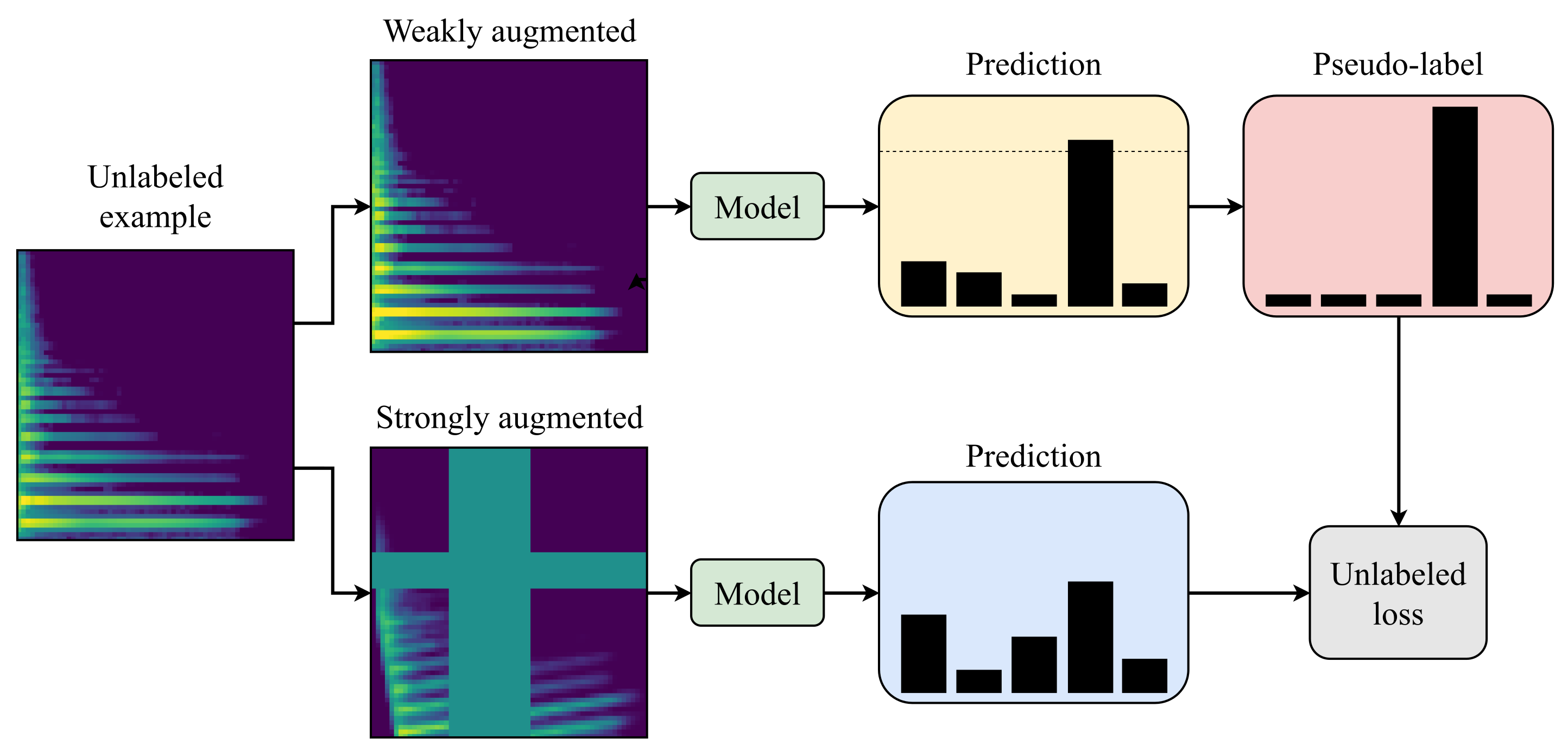
Recently, FixMatch [3] was proposed as a simplified version of MM and RMM. Only predictions from weakly augmented data with high confidence are kept as targets. Instead of sharpening the predicted distributions, the class with the highest confidence is used as the target label, comparable to the PL method. The pseudo labels are filtered with a confidence threshold (95% suggested by the authors), and only high confidence predictions are used for training. This excludes uncertain predictions in the early training phases. It also iteratively increases the amount of unlabeled data being included in the training process as the model becomes more confident in its predictions. The filtered instances are then transformed by randomly picking two strong augmentation methods from a predefined set, using a magnitude (strength of the transformation) randomly sampled for each training step. One goal for this approach is to systematically produce the same predictions for the weakly and strongly augmented unlabeled data using the CCE loss as displayed in Figure 1. The second part of the loss function, similar to PL, is the supervised performance on the weakly augmented version of the labeled dataset using CCE loss as well. In contrast to the PL approach, an additional weighting factor in the loss function is not critical to achieve good performance since the number of unlabeled examples used for training increases over time as more of them pass the threshold. FM achieved 95.7% accuracy on CIFAR-10 using 400 examples per class with the same model architecture as MM. Reducing the amount of labels per class to 25 only slightly reduced performance to 94.9%, while the performance of MT dropped to 67.7%. Using only four examples per class FM still obtained 88.6% while the performance of RMM (80.9%) and MM (52.5%) decreased considerably more, demonstrating the potential of this method in the few label domain. FM also simplified the training process by using only one strong augmentation compared to RMM. Furthermore, it was shown that randomly picking the magnitude for strong augmentations in each training step performed comparable to CTAugment (introduced for RMM) in which the best magnitude for each augmentation is learned over the course of the training.
The Meta Pseudo Labels approach by Pham et al. [4] slightly improved the upper baseline set by FM to 96.1% using 400 examples per class for CIFAR-10, but no results were reported for fewer labels. Instead of a single model, separate student and teacher models are used. First, the student learns from the pseudo labels generated by the teacher. Next, the teacher is modified depending on how well the updated student performs on the labeled part of the dataset. This should lead to an improved teacher model that generates more accurate pseudo labels for the student in every iteration. To achieve the best performance, the teacher is additionally trained with auxiliary supervised and semi-supervised objectives. Although Meta Pseudo Labels achieves a slightly higher accuracy than FM, we do not include it in this work since it requires a more complicated training procedure and no performance was reported in the low-label domain.
The SSL techniques mentioned so far were mainly developed using image classification tasks and datasets. In the following, we present a brief description of SSL methods applied to audio tasks. Consistency regularization in the form of MT was applied to SED and SCR improving the supervised model trained from scratch with few data. However, this approach did not reach the fully supervised baseline which included all annotated data [16]. Recently, Cances et al. [10] applied several SSL methods on one additional SED and the same SCR datasets as [16]. The study included the SSL methods MT, MM, and FM. When the amount of labeled examples was reduced to 10%, FM and MM outperformed MT and the supervised CNN trained from scratch. This is inline with the findings from the image domain. In contrast to [16], MT did not perform as well as the supervised baseline on all datasets. On 10% of the dataset size, FM and MM reached the fully supervised baseline which includes the complete labeled dataset (100%) on two of the three datasets confirming the potential of SSL. Further data reduction steps were not conducted. Cances et al. additionally integrated Mixup into FM in a similar way as it was used in MM. This improved results slightly on two datasets. It must be noted that the results of Lu et al. [16] and Cances et al. [10] are difficult to compare since different amounts of training data were used, and the similarity of the test set could not be confirmed. For UrbanSound8k [17] Cances et al. tested on the provided 10-fold split with only 10% reduction of training data, while Lu et al. “split the labeled data into training and test sets” with varying reduction sizes without covering the 10% reduction step.

2.2. Augmentation Methods Applied to Audio Data

Augmentation methods for audio data can be clustered into two main classes: the ones applied directly on the raw audio signal (e.g., time stretching) and methods applied after the data has been transformed to a time-frequency representation. Since FM was originally proposed to work with 2D input images, we focus on methods that can be applied during run-time to the 2D time-frequency representation of the audio signal. Augmentations applied to the raw audio signal are left for future work.
For urban sound tagging, Adapa [18] applied image augmentation techniques such as random erasing, random rotate, and grid distortion to input audio spectrograms. Color jitter and stretching of the time and frequency axes were applied, amongst others, to bird audio detection using CNNs [19]. Another successfully used augmentation technique for spectral images is SpecAugment [20], where one or more contiguous time frames and frequency bins are set to a fixed value. This is comparable to the Cutout technique [21] used in FM, as well as random erasing where one rectangular region is masked. Johnson et al. [22] applied image augmentation methods (grid distortion, random brightness, random erasing, random rotating, and SpecAugment) to ISA datasets and increased robustness of CNNs to domain shift between train and test sets. Such augmentation methods have also been successfully used for MIR tasks such as classifying the size of musical ensembles [23]. These examples demonstrate the general applicability of the proposed image augmentation methods for spectral audio data from various domains.

2.3. Transfer Learning Using Pre-Trained Embeddings

Another approach to tackle the problem of small training datasets is to pre-train models on tasks where enough data is available, and then transfer the learned knowledge to new tasks. Here, the models can be fine-tuned or intermediate feature representations, i.e., embeddings, can be extracted to train new classifiers. This alternative training paradigm should therefore be considered when evaluating the performance of SSL methods [9]. In [24], we compared several pre-trained embeddings for six audio classification tasks from the fields of MIR and ISA, including tasks such as instrument family recognition and metal ball surface classification. The OpenL3 embeddings [25] outperformed the other evaluated embeddings as well as networks trained from scratch, especially when the amount of labeled data was reduced. Furthermore, it was shown that the linear Support Vector Machine (SVM) classifier performed best on average using these embeddings as input features. OpenL3 embeddings also demonstrated their potential on SED datasets [25]. Since OpenL3 embeddings performed well over several tasks from different audio domains, we include them as an additional baseline in this work.

3. Experiments

The following section describes the selected datasets and corresponding tasks including the general processing pipeline and dataset specific supervised baselines. Then we outline the methods that are evaluated for SSL and TL. Finally, we describe the experiments on data augmentation and the full evaluation that compares the supervised baselines, SSL, and TL.

3.1. Datasets and Tasks

For a thorough evaluation of the potential of FM for audio classification, we selected three classification tasks from the fields for ISA, ASC, and MIR. Picking audio data from different domains should show the influence of varying difficulties and audio characteristics for the evaluated methods. Only publicly available datasets with a separate pre-defined test set were used. This choice was made to allow for reproducibility and to avoid time-consuming cross-validations in the experiments. Table 1 provides details of the selected datasets, which we explain with the corresponding state-of-the-art results in the following section.

3.1.1. Metal Surface Classification (MB)

From the field of ISA we selected the IDMT_ISA_METAL_BALL (MB) dataset [26]. Due to abrasion, the surface of metal balls can get damaged over time. This dataset was compiled to build classifiers that detect the surface of metal balls by their rolling sound. It contains three surface conditions: “eloxed”, “coated”, and “broken”. For further details on the dataset and recording procedure we refer to [26]. It contains pre-defined balanced train and test sets which were recorded under the exact same conditions. This shared data distribution makes this dataset the least complex one in this study. The supervised state-of-the-art baseline was reported by Johnson et al. [22], where a CNN achieved 99.6% accuracy using the full training set with 450 examples per class. With OpenL3 embeddings, a SVM classifier obtained 97.1% on the full dataset and 96.8% using only 10% of the training data [24].

3.1.2. Acoustic Scene Classification (TUT2017)

From the field of ASC, we use the TUT Urban Acoustic Scenes 2017 (TUT2017) dataset with its corresponding development (train) [27] and evaluation (test) [28] splits. It contains 10 s long stereo audio files from 15 different acoustic scenes such as grocery store or library, each recorded in several locations. The locations of training and test set do not overlap, making the classification task more challenging.
Heittola et al. [29] proposed a CNN baseline that achieved 74.8% file-wise accuracy on the development set, and 61.0% on the final test set, highlighting the difference between train and test sets, as well as the general difficulty of the task. TUT2017 was used in the 2017 IEEE AASP Challenge on Detection and Classification of Acoustic Scenes and Events (DCASE) in Task 1 “Acoustic scene classification” (http://dcase.community/challenge2017/task-acoustic-scene-classification, accessed on 27 August 2020). The best performing system obtained 83.3% on the test set using generative adversarial networks [30]. The best placed system using only CNNs trained in a supervised manner, comparable to our supervised baseline, achieved 77.7% [31] and was placed third in the challenge. This dataset was also used by Pons et al. [32] to compare several few-shot learning approaches such as prototypical networks [33] and TL. To evaluate the effectiveness of the approaches, the training set size was reduced step-wise down to one example per class. Prototypical networks performed best with more than 20 examples per class; TL was beneficial for smaller training set sizes. These results allow a comparison to our supervised, TL, and most importantly, SSL performance on this task.

3.1.3. Instrument Recognition (NSynth)

As a MIR task, we selected musical instrument family recognition using the NSynth dataset [34]. NSynth contains 300k musical notes sampled from over 1k instruments. These instruments belong to 11 instrument families such as bass, string, and vocals. It comes with a separate test set that contains only unseen instruments for each family. This makes it a more challenging dataset than MB. Since the test dataset contains no recordings for “synth_lead” we excluded this instrument family from our experiments leading to a total of 10 instrument families. The files were recorded with a sample rate of 16 kHz and a length of 4 s. For more details refer to [34]. Current supervised state-of-the-art reported a classification accuracy of 73.8% using a CNN [35]. Augmenting the raw audio data with effects such as chorus or flanger increased the accuracy to 74.7%. With pre-trained Contrastive Learning for Audio (COLA) embeddings, Saeed et al. [36] reported 73.0% with and 63.4% without fine-tuning.

3.2. Processing Pipeline

The main focus of this work is to evaluate the potential of FM for audio classification tasks. Therefore, we first implement a processing pipeline which allows us to train and test fully supervised baselines, classifiers using TL, and the SSL methods FM and MT on the same data. To avoid differences due to variations in the processing pipeline we run all experiments with the same code base and input data. For more details on on SSL evaluation practices we refer the reader to [9]. Due to randomness in training and data selection for smaller dataset sizes, results may slightly differ from those previously reported in the literature.
We use the same CNN architecture for all tasks and datasets, called CNN420 in the remainder of the paper. It is inspired by the ResNet model described in [37] using Independent-Component (IC) layers proposed by Chen et al. [38] in each ResNet block. These IC layers add additional regularization to the network by including dropout. We adapted the architecture slightly to achieve results comparable to the state of the art on all datasets for the fully supervised baseline. The final configuration is shown in Table 2. Tests on supervised training and FM using Wide ResNet28 [15] and MobileNetV2 [39] were conducted but led to similar or worse results than the ones obtained with CNN420. However, it must be noted that better architectures and hyperparameters for each individual dataset and training data size might exist. An extensive hyperparameter search was not performed. Rather than optimizing models, our aim was to have comparable results for the different experiments while remaining close to the reported state-of-the-art performance on each task. All CNN420 models are trained using Adam optimizer [40] for 70 epochs with a learning rate of 1 × 10⁻³. Learning rate schedulers did not lead to significant improvements in preliminary tests and were hence discarded in favor of model and training simplicity.

3.3. Supervised Baselines

The best results in a classification task are commonly achieved by using annotated datasets in a fully supervised training setting. In this work, we provide our own fully supervised baselines trained with the entire dataset as the upper boundary for our models and feature extraction methods. In each training batch, two augmentation methods are randomly picked with a random magnitude from all spectral augmentations that are later considered in FM (see Section 4.1). This is in line with the procedure described in [22]. All feature extraction was done using the Librosa python library [41] (version 0.8.0: https://pypi.org/project/librosa/, accessed on 27 August 2020).

3.3.1. Metal Ball

As an input representation we use the Mel-spectrogram with 64 bands. Window and hop sizes of 512 samples leads to a patch size of 34 × 64 representing one full recording. Similar to [22], no overlap between STFT windows was used. These input features and our default processing pipeline resulted in 99.4% accuracy on the test set with the CNN420. These results are comparable to the 99.6% accuracy reported in the state of the art [22].

3.3.2. TUT2017

As input features we use Mel-spectrogram with 128 bands, a window size of 2048, and a hop size of 1024 samples. The stereo channels are used similar to color channels for images. Per-channel energy normalization (PCEN) [42] is applied to each channel since it improved results on the fully supervised baseline (using implementation and default parameters from Librosa python library version 0.8.0). A total of 128 spectral frames are concatenated for one spectral image with an overlap of 64 frames. This creates five spectral images for each recording. Using the CNN420, we achieved 77.2% file-wise accuracy with majority voting over the five patches per file. These results are comparable to the ones reported in [31] with 77.7% using a CNN model.

3.3.3. NSynth

As input features, we use dB-scaled Mel-spectrogram with 64 bands, a window size of 2048, and a hop size of 1024 covering the whole audio snippet in one spectral image with 61 time frames. With the CNN420, we achieved 77.1% accuracy on the test set which is slightly higher than the previous state of the art of 74.7% [35].

3.4. Transfer Learning

TL is an alternative to SSL for training models with few annotated data and should therefore be considered as an additional baseline [9]. For TL, OpenL3 embeddings have been shown to be a good starting point for audio classification tasks, resulting in good classification results especially when the amount of labeled data available is small [24,25]. As suggested in [24], we extract OpenL3 embeddings trained on music with an output size of 512 with Mel-spectrograms as input and use a linear SVM classifier (OpenL3 embeddings were extracted with the OpenL3 python library version 0.3.1: https://pypi.org/project/openl3/, accessed on 3 March 2020).

3.5. Semi-Supervised Learning (SSL) Approaches

3.5.1. FixMatch (FM)

Our training procedure for FM is similar to the one described in [3]. As proposed by the authors, we use seven times more unlabeled than labeled data in each batch and a threshold of 0.95 for filtering the pseudo labels. The labeled batch size is set to 32, and one epoch includes all unlabeled training examples. The output of the time-frequency transform is first normalized to a range between 0 and 1 so default image augmentation methods can be directly applied. For the strong augmentation of the unlabeled data we also randomly pick two augmentations with a randomly selected magnitude. For Cutout, the best performance was achieved with a 50% rectangle size and a mask value of 0.5 which is in line with [3]. Augmentations are performed with Albumentations python library [43] (version 0.5.2: https://pypi.org/project/albumentations/, accessed on 30 November 2020). After augmentation, the data is normalized to zero mean and standard deviation of one per mel band. The normalization matrix is calculated on the entire non-augmented training dataset. We do not add Mixup to FM (as proposed by Cances et al. [10]) since it was reported to be detrimental to performance in one ASC dataset and only slightly beneficial for the other two datasets. In contrast to the original FM publication [3], applying an exponential moving average to the model weights did not improve accuracy and was therefore discarded.

3.5.2. Mean Teacher (MT)

The reported performance gap between FM and previous SSL methods such as MT was relatively large [3,10]. To validate these results, we also implemented MT as a second SSL method. We ramp up the consistency weight in the first 10 epochs to the maximum which is set to the number of classes for each dataset as suggested in [7]. For augmentation, we pick the weakest augmentations from the results of Section 4.1. This led to the best results for all tasks in preliminary experiments with 5% of the training data.

3.6. Data Augmentation

FM relies heavily on weak and strong augmentations of the input data. To distinguish which transformation can be seen as weak, the impact of each augmentation method on each dataset is measured in the following experiment. From these results we evaluate several strategies on how to select the weak augmentation method(s) for FM. This procedure is described in detail in the following sections.

3.6.1. Impact of Augmentation on Model’s Performance

Augmentation is an important component of FM. Changing or replacing weak and strong augmentations leads to a performance loss or even stopped models from converging in [3]. However, the procedure for classifying transformations between weak and strong was not described in detail in the original publication, where horizontal flipping and translation in the x and y directions were used as weak augmentations. For audio, however, translation and flipping have a different effect on the data. X translation corresponds to shifting events in time, while a translation in y changes the frequency of the audio content. Horizontal flipping is effectively the same as playing the audio backwards. While these augmentations might still be suitable for some audio use cases, they can drastically change the output in classification tasks such as instrument classification, where the temporal evolution or absolute frequency of the audio signal play a critical role. Therefore, the selection of FM augmentations when dealing with audio data needs to be carefully analyzed.
We propose a method to measure the strength of each augmentation on the performance of the model. First, the CNN420 is trained on the non-augmented labeled dataset. We use 5% of the full dataset size for the experiments since our focus is to perform classification with few labels. The trained model is then evaluated on the same augmented data. If the impact of a given transformation is minor (weak), the classification performance should be close to the one obtained with the original (non-augmented) data. In contrast, for strong augmentations a major performance drop is to be expected. All evaluated augmentation methods tested in this work are shown in Figure 2. Parameter limits for each augmentation method were set according to [3,22] if available. Methods that rely on color change between channels were excluded from the selection. The final methods and parameters can be found in Appendix B.

3.6.2. Weak Augmentation Selection for FM

With this experiment, we evaluate different strategies to select weak augmentation methods to be used within FM. This is performed on the same 5% of labeled examples from the previous experiment. We rank all augmentations from weakest to strongest based on the results of the previous experiment. To select weak augmentations, we start from the weakest first and sequentially include augmentations based on the ranking. Medium augmentations are defined to have a performance impact that is roughly halfway between the weakest and strongest augmentation. Since the single weakest augmentation only changes the prediction slightly, we also test how FM works without weak augmentations to create the weak labels. Additionally, the originally proposed (default) weak augmentations (translate in x/y direction plus horizontal flip) are also evaluated for comparison. Inline with [3], Cutout is removed from the best version to assess its impact on performance. Furthermore, we replace Cutout by the audio related SpecAugment, which masks neighboring time frames and frequency bands instead of rectangles, to show the potential of audio-related augmentations. For SpecAugment we randomly set the width of the masked time frames/frequency bands up to 33%. Using 50% of the width and height as in Cutout would result in a much larger mask, see Figure 2. From these results we select the best strategy to perform the full evaluation.

3.7. Full Evaluation

We evaluate all methods by reducing the amount of annotated examples step-wise down to 20%, 10%, 5%, and 1% of the data. For MB and TUT2017, we also further reduce the amount of data to one example per class (one-shot learning) which corresponds to 0.3% and 0.35% of the data, respectively. For NSynth, we reduce the amount of data to 0.1% which leaves nine examples per class. The amount of labels per class after each reduction is shown in Table 3. All training data (labeled and unlabeled) was used for the unlabeled part of SSL since a minor boost in performance was observed. A performance drop is to be expected by also reducing the unlabeled examples [9] but we keep this for future work. After reducing the amount of labeled data, the training features were balanced using random downsampling. We chose to discard a few examples with downsampling rather than replicating them via upsampling since the focus of this study is suitability of modern SSL methods in the low-label domain. Each experiment was repeated three times to show the influence of data variance and randomness for few labels. The supervised and Transfer Learning baselines were also computed on the reduced datasets. Validation data is not excluded for selecting the best model weights during training. Instead, all annotated data is used for training the model in the low-label domain as suggested by Pons et al. [32].

4. Results

For all experiments, we report the mean file-wise accuracy and standard deviation over the three repetitions for the full evaluation. For TUT2017 the file-wise accuracy was calculated with majority voting over all patches per file. For MB and NSynth one patch contains the whole recording, so result aggregation is not needed. Detailed results can be found in Appendix A.

4.1. Impact of Augmentation on Model’s Performance

The impact of all augmentation methods on the labeled training data itself is shown in Figure 3 for the three datasets considered. To simulate the few-label use-case, 5% of the training data was randomly chosen for the three repetitions of this experiment. As expected, the performance on the non-augmented training data (“None”) is above 98% for all datasets since this data was already seen during training. When comparing the influence of each augmentation method, it can be seen that most augmentation methods have a very different impact on each dataset. This is further analyzed in the following sections.

4.1.1. Metal Ball

The trained model obtains 100.0% accuracy on the training data. Augmenting it with multiplicative noise (99.2%), changing the contrast (95.5%), or shearing in either direction (96.5%, 97.0%) did not decrease the performance more than 5%. These methods only change the output slightly and can be called weak. Cutout (33.4%) and Gaussian noise (39.6%) on the other hand have a very strong negative impact leading nearly to random guessing (33.3%). For MB, multiplicative noise and contrast are selected as weak augmentations in Section 4.2 (in this order). Grid distortion (58.0%) and sharpening (56.4%) are the two medium augmentations.

4.1.2. TUT2017

For TUT2017, the model obtained 96.7% on the already seen training data showing that the dataset is harder to classify than MB. Only Gaussian noise (92.5%) has an impact of less than 5% while multiplicative noise (82.7%) drops by more than 10%. Already here one can see that each augmentation method has a different impact on each dataset. Grid distortion (17.6%), sharpening (19.5%), and rotating (20.2%) have the strongest influence on the performance of the CNN420. For measuring the influence of different weak augmentations in Section 4.2, Gaussian and multiplicative noise are used as weak augmentations, contrast change (57.3%), and frequency translation (47.6%) as medium augmentations.

4.1.3. NSynth

For the task of musical instrument family recognition with the NSynth dataset, CNN420 achieved 98.8% on the training data. Several augmentation methods have only a minor impact with brightness change (98.8%) and Gaussian noise (98.8%) being the weakest. Horizontal flipping (18.3%), on the other hand, results in a performance close to random guessing (10.0%). A possible reason is that the onset and offset for each note are an important part of each instrument’s sound and flipping destroys this order by reversing it. This is in contrast to MB or TUT2017 where time-stable (noise-like) signal components are also important for classification. We therefore excluded this augmentation for this dataset. For weak augmentation we selected brightness change and Gaussian noise and for medium augmentations rotation (64.2%) and sharpening (58.5%) were selected.

4.2. Weak Augmentation Selection for FM

For this experiment, several strategies for selecting the weak augmentation(s) were evaluated on the test data. Table 4 shows that picking different augmentation methods for weak augmentation changes the performance of FM. As expected, this selection plays a crucial role in the performance of FM and should therefore be carefully done depending on the dataset at hand. In general, the augmentation methods used in the original publication [3] (“Default”) do not work as well for audio data. Instead, it can be seen that picking the single weakest transformation from Section 4.1 (“1 weak”) leads to the best results overall. Interestingly, not applying any weak augmentation (“No weak”) to the pseudo labeling process led to nearly the same results (the differences can be accounted to randomness in the training process). By picking stronger transformations (“2 weak” to “2 medium”) the performance decreases for all datasets considerably. Inline with Sohn et al. [3] removing Cutout (“1 weak no Cutout”) lowers the accuracy. Replacing Cutout with SpecAugment demonstrated the best performance overall (“1 weak SpecAug”). Based on these results, this augmentation strategy is used in the following experiments.

4.3. Full Evaluation

4.3.1. Metal Ball

Figure 4 shows the results on MB with several data reduction steps for the annotated data. With 10% of the initial training data, FM achieved nearly perfect accuracy. MT and TL fell behind by 2% and 3%, respectively, but still perform better than training from scratch. This shows that all methods that include additional data into the training, either by TL or SSL, can be beneficial. Surprisingly, FM still leads to nearly perfect results using only 1% of the initial dataset (4 examples per class). In this scenario, training a CNN from scratch only achieves 68.2%, and TL as the second best option still underperformed with 87.7%. With this small amount of labeled data, MT dropped performance considerably. These results also confirm that evaluating different dataset sizes is important for SSL research since the performance might suddenly drop [9]. For one-shot learning with FM on 0.3% of the initial data, two out of three repetitions achieved nearly 100% accuracy while one dropped to 66.6% entirely misclassifying one of the classes. All others methods did not obtain more than 64.3%. In general, SSL with FM shows great potential for ISA use-cases, such as end-of-line testing in production lines, where unlabeled data is often easy to obtain but labeled data is expensive.

4.3.2. TUT2017

The full results for TUT2017 can be seen in Figure 5. All methods fail to obtain the results from the full supervised baseline (77.2%) with a reduced amount of training examples. TL proves to be the best method for all dataset sizes. MT underperforms the supervised baseline for this dataset in all experiments. This is in line with the results from Cances et al. [10] where MT was detrimental to performance compared to a ResNet trained with augmentations on SED and SCR datasets, see Section 2.1. FM, on the other hand, seems to add useful information to the model reaching better results than the purely supervised baseline for all reduction steps. During the training process we could observe that the accuracy of the pseudo labels was lower than for the other datasets leaving room for future improvements.
The performance of SSL methods is especially interesting in the few-shot domain where the amount of labeled data is small. As previously mentioned, Pons et al. [32] evaluated different few-shot learning techniques on TUT2017 with decreasing amounts of labeled data. Prototypical networks performed best for training models from scratch. For TL, the models were first trained on AudioSet [44] in a supervised fashion and then fine-tuned on the available annotated labels from TUT2017. Since different training dataset sizes were chosen, their results cannot be directly compared to ours. We therefore use our results with the next lower number of training examples for comparison, e.g., 31 vs. 50 examples per class, making it harder for our evaluated systems. The results and the amount of labeled examples per class are shown in Table 5. While our proposed TL approach with OpenL3 performed best overall, FM performed better than training networks from scratch with Prototypical networks or TL with fine-tuning (except for one-shot learning). It can be also seen that training our proposed CNN420 in a supervised fashion with strong augmentations can perform comparably to Prototypical networks, validating the strong baseline for this work. The high performance of OpenL3 embeddings for ASC is in line with the finding of the initial publication [25].

4.3.3. NSynth

Figure 6 shows the results for NSynth. FM outperforms all other methods except for the smallest dataset size where TL obtains better results. Furthermore, it reaches the supervised baseline (77.1%) with only 5% of the initial training data while all other methods dropped by at least 7%. The gap between FM and the other methods is even larger with only 1% of the data. With 0.1% all methods except TL showed a major performance drop close to the random baseline so no further data reduction was evaluated. MT performs comparably to the supervised system for this task. TL, on the other hand, only performs well with the smallest amount of training examples. The task of instrument family recognition seems to be challenging for OpenL3 embeddings. This is line with the results reported in [24] using OpenL3 embeddings for instrument classification but with a different dataset (84.5% (best) vs. 71.4% (OpenL3)). Somehow, the differences between the instruments are not fully captured or the low sampling rate of 16kHz might be problematic. Therefore, it must be noted that other pre-trained models might improve these TL results. However, in [24] the best TL approach did not reach the fully supervised results when reducing the number of labeled examples (100% for all training data vs. 84.5% for 10% of training data). For more information we refer to the extended results of [24] with the focus on T2: https://acmus-mir.github.io/embeddings-20/, accessed on 18 January 2021.

5. Conclusions

To evaluate the potential of the Semi-Supervised Learning (SSL) method FixMatch (FM), we selected datasets from the three very different audio domains: Industrial Sound Analysis (ISA), Acoustic Scene Classification (ASC), and Music Information Retrieval (MIR). Our results showed that the selection of augmentation methods is critical for FM. Therefore, we propose a method to select those transformations by training a model on non-augmented data and testing the performance on augmented versions of it. Overall, picking the single weakest augmentation and combining it with SpecAugment, instead of the initially proposed Cutout, led to the best results. The best FM configuration for each dataset was compared to supervised training from scratch, Transfer Learning (TL) with OpenL3 embeddings, and SSL learning with Mean Teacher (MT). In contrast to MT, the proposed FM approach always improved on the baseline system that was trained from scratch on the same amount of labeled data. For MIR and ISA tasks, FM even reached the performance of the upper baseline from the full dataset with less than 5% of the labels. Only for the most difficult dataset from ASC did FM not reach the full supervised baseline and was outperformed by TL. For future work, we want to combine TL with FM. This should lower the influence of random network weights at the beginning of training and could reduce the confirmation bias added by wrong pseudo labels. The pseudo-label accuracy could be additionally improved by measuring the uncertainty of the pseudo labels predictions as recently proposed by Rizve et al. [5]. Another possible direction would be to focus on augmenting the raw audio data, for example, with pitch shifting or audio effects, instead of augmenting only the extracted spectrograms. We also did not investigate the amount of unlabeled data that is required for FM for these datasets nor possible problems with out-of-distribution examples in the unlabeled dataset and how to avoid them.

Author Contributions

S.G. substantially contributed to this work, including the formalization of the problem and experiments, the development of the ideas, implementing the approaches, conducting the experiments, and the writing of the paper. E.C. contributed to the formalization of the problem and experiments and the writing of the paper. Both authors have read and agreed to the published version of the manuscript.

Funding

This work has been supported by the German Research Foundation (BR 1333/20-1, CA 2096/1-1).

Institutional Review Board Statement

Not applicable.

Informed Consent Statement

Not applicable.

Data Availability Statement

The IDMT_ISA_METAL_BALL (MB) dataset [26], as described in Section 3.1.1, is publicly accessible under https://www.idmt.fraunhofer.de/en/publications/isa-metal-balls.html, accessed on 24 September 2019. The TUT Urban Acoustic Scenes 2017 (TUT2017) dataset [27,28], as described in Section 3.1.2, is publicly accessible under https://zenodo.org/record/400515 (train) and https://zenodo.org/record/1040168 (test), accessed on 27 August 2020. The NSynth dataset [34], as described in Section 3.1.3, is publicly accessible under https://magenta.tensorflow.org/datasets/nsynth, accessed on 8 April 2017.

Acknowledgments

The authors would like to thank David Johnson, Jakob Abeßer, Judith Liebetrau, and Thomas Köllmer for their valuable feedback during several stages of this work.

Conflicts of Interest

The authors declare no conflict of interest.

Abbreviations

The following abbreviations are used in this manuscript:
ASCAcoustic Scene Classification
CCCECategorical Cross-entropy
CNNConvolutional Neural Network
FMFixMatch
ICIndependent-Component
ISAIndustrial Sound Analysis
MBMetal Ball
MIRMusic Information Retrieval
MMMixMatch
MTMean Teacher
PLPseudo-Label
RMMReMixMatch
SCRSpeech Command Recognition
SEDSound Event Detection
SSLSemi-Supervised Learning
SVMSupport Vector Machine
TLTransfer Learning
TUT2017TUT Urban Acoustic Scenes 2017

Appendix A. Detailed Results

The following tables contain the detailed results which have been discussed in Section 4.3 with the mean accuracy and standard deviation for all repetitions. The columns for “test” are obtained from the official evaluation set while “val” refers to the unlabeled part which has been evaluated additionally. Results on the unlabeled data show the classification performance drop between data from exactly the same domain to the more difficult test domain, especially for TUT2017 and NSynth where recording scenes and instruments differ between training and test set. In Table A3, “Out of memory” refers to the SVM implementation of Sklearn (version 0.24.0: https://pypi.org/project/scikit-learn/, accessed on 5 January 2021) which ran out of memory during training. Since this result is not the focus of the work, no further action was taken.
Table A1. Detailed results for MB dataset from Figure 4 with file-wise accuracy and standard deviation on test set (test) and unlabeled training set (val).
MBFM TestFM ValSupervised TestSupervised ValTL TestTL ValMT TestMT Val
100% 99.4 ± 0.0 98.8 ± 0.0
20%100.0 ± 0.099.5 ± 0.094.9 ± 1.995.5 ± 0.897.7 ± 1.098.0 ± 0.098.4 ± 0.698.3 ± 0.4
10%99.6 ± 0.399.1 ± 0.288.7 ± 1.588.5 ± 4.396.1 ± 1.297.5 ± 0.397.9 ± 0.697.0 ± 0.3
5%99.8 ± 0.399.1 ± 0.387.1 ± 2.485.1 ± 1.395.9 ± 1.395.9 ± 0.896.3 ± 1.494.9 ± 0.8
1%100.0 ± 0.099.1 ± 0.068.2 ± 5.767.2 ± 6.687.7 ± 2.589.4 ± 0.744.1 ± 15.243.7 ± 14.4
0.3%89.7 ± 14.688.1 ± 15.762.0 ± 18.159.6 ± 17.864.3 ± 18.069.2 ± 18.233.3 ± 0.033.3 ± 0.0
Table A2. Detailed results for TUT2017 dataset from Figure 5 with file-wise accuracy and standard deviation on test set (test) and unlabeled training set (val).
TUT2017FM TestFM ValSupervised TestSupervised ValTL TestTL ValMT TestMT Val
100% 77.2 ± 0.0 74.9 ± 0.0
20%70.9 ± 0.785.5 ± 0.768.6 ± 1.079.8 ± 0.671.8 ± 0.591.1 ± 0.464.6 ± 1.371.2 ± 1.5
10%65.12 ± 1.078.6 ± 0.462.4 ± 1.469.4 ± 0.871.1 ± 1.287.9 ± 0.552.4 ± 3.053.9 ± 5.0
5%61.2 ± 2.574.2 ± 1.651.1 ± 2.056.6 ± 0.667.9 ± 1.182.8 ± 1.345.3 ± 2.141.4 ± 3.5
1%44.6 ± 3.552.2 ± 5.330.3 ± 2.931.8 ± 1.150.4 ± 4.362.8 ± 2.319.8 ± 4.216.5 ± 1.1
0.35%23.5 ± 2.232.4 ± 1.618.5 ± 3.320.6 ± 2.037.8 ± 6.446.3 ± 2.39.7 ± 1.78.9 ± 1.2
Table A3. Detailed results for NSynth dataset from Figure 6 with file-wise accuracy and standard deviation on test set (test) and unlabeled training set (val).
NSynthFM TestFM ValSupervised TestSupervised ValTL TestTL ValMT TestMT Val
100% 77.1 ± 0.0 Out of memory
20%77.4 ± 0.395.1 ± 0.275.2 ± 0.488.1 ± 0.153.9 ± 0.055.9 ± 0.074.8 ± 0.692.4 ± 0.5
10%76.9 ± 0.692.5 ± 0.372.9 ± 0.682.6 ± 0.153.9 ± 0.055.8 ± 0.073.5 ± 0.386.4 ± 0.1
5%75.8 ± 0.588.3 ± 0.170.4 ± 0.673.7 ± 0.353.8 ± 0.055.6 ± 0.068.2 ± 1.377.0 ± 0.8
1%71.0 ± 1.974.0 ± 1.954.2 ± 1.052.4 ± 1.452.6 ± 0.054.2 ± 0.048.5 ± 3.749.0 ± 3.8
0.1%25.4 ± 0.927.6 ± 0.822.4 ± 1.526.3 ± 0.445.4 ± 0.946.9 ± 0.223.4 ± 1.621.5 ± 2.0

Appendix B. Augmentation Details

Table A4 shows all augmentations methods that were considered in this study for either supervised or SSL training. The magnitudes of each transformation were picked randomly up to the limit which was set according to [3,22] if available.
Table A4. Augmentation methods with corresponding parameter limits.
MethodParameters
BrightnessLimit: 0.025
ContrastLimit: 0.5
SharpenAlpha: 0.5, lightness: 0
Shear xLimit: 1.0
Shear yLimit: 1.0
RotateLimit: 10
Translate freq.Limit: 12.5%
Translate timeLimit: 12.5%
Translate freq. & timeLimit: 12.5%
Horiz. flip-
Grid distortionDefault
Gaussian noiseLimit: 0.0001
Multiplicative noiseLimit: 0.8–1.2
CutoutSize: 50%
SpecAugmentSize time and freq mask: 33%

References

  1. Berthelot, D.; Carlini, N.; Goodfellow, I.; Papernot, N.; Oliver, A.; Raffel, C.A. MixMatch: A Holistic Approach to Semi-Supervised Learning. In NeurIPS; Wallach, H., Larochelle, H., Beygelzimer, A., d’Alché-Buc, F., Fox, E., Garnett, R., Eds.; Curran Associates, Inc.: Red Hook, NY, USA, 2019; pp. 5049–5059. [Google Scholar]
  2. Berthelot, D.; Carlini, N.; Cubuk, E.D.; Kurakin, A.; Sohn, K.; Zhang, H.; Raffel, C. ReMixMatch: Semi-Supervised Learning with Distribution Alignment and Augmentation Anchoring. arXiv 2019, arXiv:1911.09785. [Google Scholar]
  3. Sohn, K.; Berthelot, D.; Carlini, N.; Zhang, Z.; Zhang, H.; Raffel, C.A.; Cubuk, E.D.; Kurakin, A.; Li, C.L. FixMatch: Simplifying Semi-Supervised Learning with Consistency and Confidence. In Advances in Neural Information Processing Systems; Larochelle, H., Ranzato, M., Hadsell, R., Balcan, M.F., Lin, H., Eds.; Curran Associates Inc.: Red Hook, NY, USA, 2020; Volume 33, pp. 596–608. [Google Scholar]
  4. Pham, H.; Dai, Z.; Xie, Q.; Luong, M.T.; Le, Q.V. Meta Pseudo Labels. arXiv 2020, arXiv:2003.10580. [Google Scholar]
  5. Rizve, M.N.; Duarte, K.; Rawat, Y.S.; Shah, M. In Defense of Pseudo-Labeling: An Uncertainty-Aware Pseudo-label Selection Framework for Semi-Supervised Learning. In Proceedings of the International Conference on Learning Representations, Virtual Conference, 3–7 May 2021. [Google Scholar]
  6. Krizhevsky, A. Learning Multiple Layers of Features from Tiny Images; Technical Report; University of Toronto: Toronto, ON, Canada, 2009. [Google Scholar]
  7. Tarvainen, A.; Valpola, H. Mean teachers are better role models: Weight-averaged consistency targets improve semi-supervised deep learning results. In Proceedings of the 31st International Conference on Neural Information Processing Systems (NIPS’17), Long Beach, CA, USA, 4–9 December 2017; pp. 1195–1204. [Google Scholar]
  8. Lee, D.H. Pseudo-Label: The Simple and Efficient Semi-Supervised Learning Method for Deep Neural Networks. In Proceedings of the ICML 2013 Workshop: Challenges in Representation Learning (WREPL), Atlanta, GA, USA, 16–21 June 2013. [Google Scholar]
  9. Oliver, A.; Odena, A.; Raffel, C.A.; Cubuk, E.D.; Goodfellow, I. Realistic Evaluation of Deep Semi-Supervised Learning Algorithms. In Proceedings of the 32nd International Conference on Neural Information Processing Systems (NIPS’18), Montréal, QC, Canada, 3–8 December 2018; pp. 3239–3250. [Google Scholar]
  10. Cances, L.; Labbé, E.; Pellegrini, T. Improving Deep-learning-based Semi-supervised Audio Tagging with Mixup. arXiv 2021, arXiv:2102.08183. [Google Scholar]
  11. van Engelen, J.E.; Hoos, H.H. A survey on semi-supervised learning. Mach. Learn. 2020, 109, 373–440. [Google Scholar] [CrossRef] [Green Version]
  12. Arazo, E.; Ortego, D.; Albert, P.; O’Connor, N.E.; McGuinness, K. Pseudo-Labeling and Confirmation Bias in Deep Semi-Supervised Learning. In Proceedings of the 2020 International Joint Conference on Neural Networks (IJCNN), Glasgow, UK, 19–24 July 2020; pp. 1–8. [Google Scholar] [CrossRef]
  13. Sajjadi, M.; Javanmardi, M.; Tasdizen, T. Regularization With Stochastic Transformations and Perturbations for Deep Semi-Supervised Learning. In Proceedings of the 30th International Conference on Neural Information Processing Systems (NIPS’16), Barcelona, Spain, 5–10 December 2016; NIPS’16; pp. 1163–1171. [Google Scholar]
  14. Zhang, H.; Cisse, M.; Dauphin, Y.N.; Lopez-Paz, D. mixup: Beyond Empirical Risk Minimization. In Proceedings of the International Conference on Learning Representations (ICLR), Vancouver, BC, Canada, 30 April–3 May 2018. [Google Scholar]
  15. Zagoruyko, S.; Komodakis, N. Wide Residual Networks. arXiv 2017, arXiv:1605.07146. [Google Scholar]
  16. Lu, K.; Foo, C.S.; Teh, K.K.; Tran, H.D.; Chandrasekhar, V.R. Semi-Supervised Audio Classification with Consistency-Based Regularization. In Proceedings of the Interspeech 2019, Graz, Austria, 15–19 September 2019; pp. 3654–3658. [Google Scholar] [CrossRef] [Green Version]
  17. Salamon, J.; Jacoby, C.; Bello, J.P. A Dataset and Taxonomy for Urban Sound Research. In Proceedings of the 22nd ACM International Conference on Multimedia (ACM-MM’14), Orlando, FL, USA, 3–7 November 2014; pp. 1041–1044. [Google Scholar]
  18. Adapa, S. Urban Sound Tagging Using Convolutional Neural Networks. Technical Report. In Proceedings of the Detection and Classification of Acoustic Scenes and Events 2019 Workshop (DCASE2019), New York, NY, USA, 25–26 October 2019. [Google Scholar] [CrossRef]
  19. Lasseck, M. Acoustic Bird Detection with Deep Convolutional Neural Networks. Technical Report. In Proceedings of the Detection and Classification of Acoustic Scenes and Events 2018 Workshop (DCASE2018), Surrey, UK, 30 March–31 July 2018. [Google Scholar]
  20. Park, D.S.; Chan, W.; Zhang, Y.; Chiu, C.C.; Zoph, B.; Cubuk, E.D.; Le, Q.V. SpecAugment: A Simple Augmentation Method for Automatic Speech Recognition. In Proceedings of the Interspeech, Graz, Austria, 15–19 September 2019. [Google Scholar]
  21. DeVries, T.; Taylor, G.W. Improved Regularization of Convolutional Neural Networks with Cutout. arXiv 2017, arXiv:1708.04552. [Google Scholar]
  22. Johnson, D.; Grollmisch, S. Techniques Improving the Robustness of Deep Learning Models for Industrial Sound Analysis. In Proceedings of the 28th European Signal Processing Conference 2020 (EUSIPCO), Virtual Conference, 18–22 January 2021. [Google Scholar]
  23. Grollmisch, S.; Cano, E.; Mora-Ángel, F.; López Gil, G. Ensemble Size Classification in Colombian Andean String Music Recordings. In Perception, Representations, Image, Sound, Music; Kronland-Martinet, R., Ystad, S., Aramaki, M., Eds.; Springer International Publishing: Basel, Switzerland, 2021; pp. 60–74. [Google Scholar]
  24. Grollmisch, S.; Cano, E.; Kehling, C.; Taenzer, M. Analyzing the Potential of Pre-Trained Embeddings for Audio Classification Tasks. In Proceedings of the 28th European Signal Processing Conference 2020 (EUSIPCO), Virtual Conference, 18–22 January 2021. [Google Scholar]
  25. Cramer, J.; Wu, H.H.; Salamon, J.; Bello, J.P. Look, Listen, and Learn More: Design Choices for Deep Audio Embeddings. In Proceedings of the IEEE International Conference on Acoustics, Speech and Signal Processing (ICASSP), Brighton, UK, 12–17 May 2019; pp. 3852–3856. [Google Scholar] [CrossRef]
  26. Grollmisch, S.; Abeßer, J.; Liebetrau, J.; Lukashevich, H. Sounding Industry: Challenges and Datasets for Industrial Sound Analysis. In Proceedings of the 27th European Signal Processing Conference 2019 (EUSIPCO), A Coruña, Spain, 2–6 September 2019. [Google Scholar]
  27. Mesaros, A.; Heittola, T.; Virtanen, T. TUT Acoustic Scenes 2017, Development Dataset, 2017. Available online: https://zenodo.org/record/400515 (accessed on 27 August 2020). [CrossRef]
  28. Mesaros, A.; Heittola, T.; Virtanen, T. TUT Acoustic Scenes 2017, Evaluation Dataset, 2017. Available online: https://zenodo.org/record/1040168 (accessed on 27 August 2020). [CrossRef]
  29. Heittola, T.; Mesaros, A.; Diment, A.; Elizalde, B.; Shah, A.; Vincent, E.; Raj, B.; Virtanen, T. DCASE 2017 Challenge Setup: Tasks, Datasets and Baseline System. In Proceedings of the Detection and Classification of Acoustic Scenes and Events 2017 Workshop (DCASE2017), Munich, Germany, 15 March–31 July 2017. [Google Scholar]
  30. Mun, S.; Park, S.; Han, D.; Ko, H. Generative Adversarial Network Based Acoustic Scene Training Set Augmentation and Selection Using SVM Hyper-Plane. Technical Report. In Proceedings of the Detection and Classification of Acoustic Scenes and Events 2017 Workshop (DCASE2017), Munich, Germany, 15 March–31 July 2017. [Google Scholar]
  31. Weiping, Z.; Jiantao, Y.; Xiaotao, X.; Xiangtao, L.; Shaohu, P. Acoustic Scene Classification Using Deep Convolutional Neural Network and Multiple Spectrograms Fusion. Technical Report. In Proceedings of the Detection and Classification of Acoustic Scenes and Events 2017 Workshop (DCASE2017), Munich, Germany, 15 March–31 July 2017. [Google Scholar]
  32. Pons, J.; Serrà, J.; Serra, X. Training Neural Audio Classifiers with Few Data. In Proceedings of the IEEE International Conference on Acoustics, Speech and Signal Processing (ICASSP), Brighton, UK, 12–17 May 2019; pp. 16–20. [Google Scholar] [CrossRef] [Green Version]
  33. Snell, J.; Swersky, K.; Zemel, R. Prototypical Networks for Few-shot Learning. In Advances in Neural Information Processing Systems; Guyon, I., Luxburg, U.V., Bengio, S., Wallach, H., Fergus, R., Vishwanathan, S., Garnett, R., Eds.; Curran Associates Inc.: Red Hook, NY, USA, 2017; Volume 30. [Google Scholar]
  34. Engel, J.; Resnick, C.; Roberts, A.; Dieleman, S.; Norouzi, M.; Eck, D.; Simonyan, K. Neural Audio Synthesis of Musical Notes with WaveNet Autoencoders. In Proceedings of the 34th International Conference on Machine Learning, Sydney, Australia, 6–11 August 2017; pp. 1068–1077. [Google Scholar]
  35. Ramires, A.; Serra, X. Data augmentation for instrument classification robust to audio effects. In Proceedings of the 22nd International Conference on Digital Audio Effects (DAFx-19), Birmingham, UK, 2–6 September 2019. [Google Scholar]
  36. Saeed, A.; Grangier, D.; Zeghidour, N. Contrastive Learning of General-Purpose Audio Representations. arXiv 2020, arXiv:2010.10915. [Google Scholar]
  37. Johnson, D.S.; Lorenz, W.; Taenzer, M.; Mimilakis, S.; Grollmisch, S.; Abeßer, J.; Lukashevich, H. DESED-FL and URBAN-FL: Federated Learning Datasets for Sound Event Detection. arXiv 2021, arXiv:2102.08833. [Google Scholar]
  38. Chen, G.; Chen, P.; Shi, Y.; Hsieh, C.Y.; Liao, B.; Zhang, S. Rethinking the Usage of Batch Normalization and Dropout in the Training of Deep Neural Networks. arXiv 2019, arXiv:1905.05928. [Google Scholar]
  39. Sandler, M.; Howard, A.; Zhu, M.; Zhmoginov, A.; Chen, L.C. MobileNetV2: Inverted Residuals and Linear Bottlenecks. In Proceedings of the IEEE Conference on Computer Vision and Pattern Recognition (CVPR), Salt Lake City, UT, USA, 18–22 June 2018. [Google Scholar]
  40. Kingma, D.P.; Ba, J. Adam: A Method for Stochastic Optimization. In Proceedings of the International Conference on Learning Representations (ICLR), San Diego, CA, USA, 7–9 May 2015. [Google Scholar]
  41. McFee, B.; Lostanlen, V.; Metsai, A.; McVicar, M.; Balke, S.; Thomé, C.; Raffel, C.; Zalkow, F.; Malek, A.; Lee, K.; et al. Librosa/Librosa: 0.8.0. 2020. Available online: https://librosa.org/ (accessed on 27 August 2020). [CrossRef]
  42. Wang, Y.; Getreuer, P.; Hughes, T.; Lyon, R.F.; Saurous, R.A. Trainable frontend for robust and far-field keyword spotting. In Proceedings of the IEEE International Conference on Acoustics, Speech and Signal Processing (ICASSP), New Orleans, LA, USA, 5–9 March 2017; pp. 5670–5674. [Google Scholar]
  43. Buslaev, A.; Iglovikov, V.I.; Khvedchenya, E.; Parinov, A.; Druzhinin, M.; Kalinin, A.A. Albumentations: Fast and Flexible Image Augmentations. Information 2020, 11, 125. [Google Scholar] [CrossRef] [Green Version]
  44. Gemmeke, J.F.; Ellis, D.P.W.; Freedman, D.; Jansen, A.; Lawrence, W.; Moore, R.C.; Plakal, M.; Ritter, M. Audio Set: An ontology and human-labeled dataset for audio events. In Proceedings of the IEEE International Conference on Acoustics, Speech and Signal Processing (ICASSP), New Orleans, LA, USA, 5–9 March 2017; pp. 776–780. [Google Scholar]
Figure 1. Schematic representation of FM training process for the unlabeled part of the dataset. The model generates a hard label on weakly augmented versions of an unlabeled example. The model is then trained to output the same label for a strongly augmented version of the example. Figure modified from [3].
Electronics 10 01807 g001
Figure 2. All augmentation techniques with random magnitude applied to one example from the NSynth dataset with mel bands on the y (0 to 64) and time frames on the x axis (beginning to the end of the recording).
Electronics 10 01807 g002
Figure 3. Mean accuracy and standard deviation for all augmentation methods on 5% of the labeled training data of each dataset.
Electronics 10 01807 g003
Figure 4. Mean accuracy and standard deviation for FixMatch (FM), fully supervised training (Supervised), Transfer Learning (TL), and Mean Teacher (MT) on MB test set. Additionally, the supervised baseline using the full training set (Full) and the random baseline are shown.
Electronics 10 01807 g004
Figure 5. Mean accuracy and standard deviation for FixMatch (FM), fully supervised training (Supervised), Transfer Learning (TL), and Mean Teacher (MT) on TUT2017 test set. Additionally, the supervised baseline using the full training set (Full) and the random baseline are shown.
Electronics 10 01807 g005
Figure 6. Mean accuracy and standard deviation for FixMatch (FM), fully supervised training (Supervised), Transfer Learning (TL), and Mean Teacher (MT) on NSynth test set. Additionally, the supervised baseline using the full training set (Full) and the random baseline are shown.
Electronics 10 01807 g006
Table 1. Dataset details including the number of classes, total amount of files for training and testing, the file duration (File dur.) of each audio recording, the sample rate, and the number of channels of the audio data.
TaskClassesTrainTestFile Dur. (s)Sample Rate (kHz)Channels
MB31350171144.11
TUT201715468016201044.12
NSynth10300k40964161
Table 2. CNN420 Resnet Architecture with 420k parameters and average (avg.) pooling between ResNet blocks. Details on the ResNet block are explained in [37].
LayerOutputKernel SizeDropout
Conv 2D64(5, 5)-
Relu---
ResNet Block64(3, 1)0.10
Avg. Pooling-(2, 2)-
ResNet Block64(3, 3)0.10
Avg. Pooling-(2, 2)-
ResNet Block64(3, 3)0.10
ResNet Block128(3, 1)0.10
Avg. Pooling-(2, 2)-
ResNet Block256(1, 1)0.10
Avg. Global Pooling---
SoftmaxNr. of classes--
Table 3. Percentage and number of labeled examples per dataset.
Task100%20%10%5%1%0.3%0.1%
MB45090452241-
TUT201731262311531-
NSynth8773175587743987-9
Table 4. Results for different weak augmentation strategies on the test data of each dataset with 5% of the training data, including default (similar to [3]), no weak augmentations, and one or two weak/medium (med.) augmentations applied.
DatasetDefaultNo Weak1 Weak2 Weak1 Med.2 Med.1 Weak
No Cutout
1 Weak
SpecAug
MB94.15100.099.8199.2297.6693.9695.3299.42
TUT201761.1162.0461.4260.0655.1956.7955.6264.26
NSynth69.0475.2075.1073.2771.8372.3174.0276.10
Table 5. Comparison of classification accuracy to Prototypical Networks (Prot. Net.) and TL with fine-tuning (TL-ft) reported in [32]. For a fair comparison, the next lower amount of labeled examples per class (“Examples”) from our experiments is considered.
ExamplesFMSuperv.TLExamples [32]Prot. Net. [32]TL-ft [32]
6270.968.671.810067.860.6
3165.162.471.15062.058.8
1558.351.167.92053.854.0
344.630.350.4535.446.1
123.518.537.8118.235.2
Publisher’s Note: MDPI stays neutral with regard to jurisdictional claims in published maps and institutional affiliations.

