Data-Driven Channel Pruning towards Local Binary Convolution Inverse Bottleneck Network Based on Squeeze-and-Excitation Optimization Weights

Abstract

This paper proposed a model pruning method based on local binary convolution (LBC) and squeeze-and-excitation (SE) optimization weights. We first proposed an efficient deep separation convolution model based on the LBC kernel. By expanding the number of LBC kernels in the model, we have trained a larger model with better results, but more parameters and slower calculation speed. Then, we extract the SE optimization weight value of each SE module according to the data samples and score the LBC kernel accordingly. Based on the score of each LBC kernel corresponding to the convolution channel, we performed channel-based model pruning, which greatly reduced the number of model parameters and accelerated the calculation speed. The model pruning method proposed in this paper is verified in the image classification database. Experiments show that, in the model using the LBC kernel, as the number of LBC kernels increases, the recognition accuracy will increase. At the same time, the experiment also proved that the recognition accuracy is maintained at a similar level in the small parameter model after channel-based model pruning by the SE optimization weight value.

1. Introduction

With the development and wide application of deep learning, the field of artificial intelligence has undergone tremendous changes in recent years. Owing to higher requirements for model results, deeper and more complex deep learning network structures are proposed [1,2,3,4,5,6,7]. What follows is exponential growth in model parameters and memory requirements, which makes it difficult to implement to various hardware platforms, such as mobile devices [8,9,10]. To improve the calculation speed of the model, in addition to further improving the calculation speed of the hardware, many researchers also try to reduce the number of parameters required by changing the model structure [8,10,11,12,13]. Moreover, some researchers have focused on the methods of model compression to modify the trained model and compress it to minimize the computational space and time consumption of the model [14,15,16,17]. Model pruning is a type of model compression [18,19,20,21]. It is based on an assumption, or the current consensus, which is the over-parameterization of deep neural networks [22,23]. Over-parameterization means that we need a lot of parameters in the training phase to capture the tiny information in the data, and once the training is completed to the inference phase, we do not need so many parameters. This assumption supports that we can simplify the model before deployment.

Through pruning at different granularities of model parameters, model pruning methods can be divided into unstructured pruning [18,19,21,24,25] and structured pruning [20,26,27]. In unstructured pruning, the weights of the network are pruned at the neuron level. This pruning method has the highest flexibility, but it will cause the weight matrix to be sparse, requiring additional sparse matrix operation libraries or specially designed hardware support [28]. Compared with unstructured pruning, the structured pruning algorithm does not require additional computing library support and is more user-friendly in terms of implementation and deployment. Structured pruning is used to prune the model's filter or channel granularity. By scoring the filter or channel of the model, the parts with lower scores are removed, thereby reducing the model parameters. The structured pruning method is more of an optimization of the model structure. In the work of [29], it is pointed out that, after pruning, the more important thing is the preservation of the model structure rather than its parameters. From this point of view, the structured pruning method is also a neural architecture search (NAS) [30], but, because it only involves layer dimensions, the search space is smaller.

In recent studies, the attention mechanism has been widely used in Convolutional Neural Network (CNN). From the spatial attention mechanism [31,32,33,34,35,36], channel attention mechanism [37], and part of the research used a mixed attention mechanism [38,39,40]. The attention mechanism itself calculates the features extracted by the model and adds more weight to the more important features of the result. SEnet [37] proposed the process of dividing the channel-based attention mechanism into a squeeze, excitation, and scale, adding more non-linear calculations to the channel-based attention mechanism, which provided the basis for many subsequent studies. Compared with the previously mentioned evaluation method of model pruning, the attention weight of different parts of the model is also the evaluation of the intermediate features extracted by the model. This evaluation is data-driven and can be expressed through intuitive scores. At the same time, most of the attention mechanism methods rely on the training in the model, and the attention weight corresponding to the data sample changes greatly in the process of pruning and retraining.

In this context, we thought of the LBC network [41]. LBC is an application based on local binary pattern (LBP) [42] features in traditional machine learning and uses a non-trainable convolution kernel with only three values of −1, 0, and 1. The convolution kernel of LBC is binarized and has advantages over traditional convolution kernels in terms of calculation speed and storage space. In the case of the same convolution kernel size, the non-trainable convolution kernel parameters reduce the overall training difficulty of the model. However, because the LBC kernel is not trainable, the model result has a great correlation with the number of kernels. As the effect of LBC has a strong positive correlation with the number of LBC kernels, many randomly generated LBC kernels must be redundant. This assumption is in line with the theory of model pruning. Model pruning based on LBC not only needs to find the model structure after pruning, but it is more important to find the non-trainable LBC kernel parameters. In our work, we did not use the existing structured model pruning scoring method, but used the weight of the data-driven SE block as the evaluation of the channel. At the same time, a depthwise convolution layer structure is introduced, so that the LBC kernel corresponds to the SE optimization weight. Compared with the evaluation function of the existing model pruning method, the squeeze-and-excitation (SE) optimization [37] weight is obtained through training, and the relationship with the convolution channel is more intuitive.

In our paper, we propose a basic network structure based on mobile inverted bottleneck [12,43,44] convolutional layer and squeeze-and-excitation optimization. By changing its inverted bottleneck expand ratio, the number of LBC kernels in each LBC layer is adjusted. By training large models and using pruning methods, we get models with smaller calculations and higher accuracy. Figure 1 shows our expansion-pruning process. We conducted experiments on the image classification database CIFAR-10 [45]. The result proves the effectiveness of our proposed method; in the models with smaller expand ratios, its recognition accuracy still maintains the same level.

2. Related Work

With the good results of deep neural networks in various fields, the computing resources required by the model also increase. Model size, memory footprint, number of calculation operations (FLOPs), and power consumption are the main aspects that hinder the use of deep neural networks in certain resource-constrained environments. Those large models may not be stored and cannot be run in real-time on embedded systems. To solve this problem, many methods have been proposed, such as low-rank approximation of weights [4,46], weight quantization [47,48], knowledge distillation [49], and model pruning, where model pruning has attracted much attention thanks to its competitive performance and compatibility.

In the work of the early 1990s, when the weight is set to zero, the second-order Taylor approximation method with an increased network loss function is used for pruning. In optimal brain damage [18], the saliency for each parameter was computed using a diagonal Hessian approximation, and the low saliency parameters were pruned from the network, and the network is retrained. In optimal brain surgeon [19], the saliency of each parameter was calculated using the inverse Hessian matrix, the low saliency weight was pruned, and all other weights in the network were updated with second-order information. More recently, another paper [24] proposed to trim the weight of the network to a small extent, and further integrate this technology into the deep compression pipeline [28] to obtain a highly compressed model. Besides, many researchers have proposed various algorithms to iteratively remove redundant neurons, use Variational Dropout to trim excess weights [50], and learn sparse networks through regularization of the L0 paradigm based on random gates [25]. But, one disadvantage of these unstructured pruning methods is that the resulting weight matrix is sparse, and if there is no dedicated hardware/library, it cannot cause compression and acceleration [28].

In contrast, the structured pruning method is pruning at the channel or even at the level. As the original convolution structure is still retained, no dedicated hardware/library is required to achieve these benefits. Among the structured pruning methods, channel pruning [22,51,52] is the most popular method because it operates at the most granular level while still being suitable for conventional deep learning frameworks. There are three classic ideas for the channel pruning algorithm. The first is based on the importance factor [52], that is, to evaluate the effectiveness of a channel, and to constrain some channels to make the model structure itself sparse, so that pruning is based on this. The second is to use reconstruction errors to guide pruning [22,51], indirectly measuring the impact of a channel on the output. The third is to measure the sensitivity of the channel based on the change of the optimization target. However, the work of [29] pointed out that, for structured pruning, after obtaining the compression model through the pruning algorithm, it is better to initialize and train the compression model randomly instead of using the weights of the large network for fine-tuning. For the final compressed small model, the network architecture obtained by the pruning algorithm is more important than the "important" weight obtained by the pruning. The model through the pruning algorithm can provide design guidance for designing an effective network architecture. For most convolutional neural networks, fine-tuned convolution kernels from large networks are more likely to cause the model to fall into overfitting.

Similar to the method of scoring the part of the model that needs to be cut in model pruning, the attention mechanism method widely used in image processing and image sequence processing [53] is used to evaluate the intermediate features extracted by the model. In CNN, based on the original attention mechanism applied to the human visual system [31,32], the spatial attention mechanism was applied to it very early. For example, in the original picture information, focus on the area that needs more attention [33,34,35], and find the relationship weight of any pixel in the image to the current pixel from the global information [36]. In addition to spatial attention, many studies have focused on the attention mechanism of the convolution channel [37] in CNN. In the work of [37], they use global average-pooled features to compute channel-wise attention. Spatial attention puts more weight on the input image, and according to different input images, more information parts will be found. The channel attention is more about weighting the convolution kernel. Corresponding to different input images, a specific convolution kernel can find important information more of the time.

In our work, we use the LBC kernel [41] to replace the general convolution kernel and perform structured pruning to avoid the above problems. The LBC is inspired by the LBP [42] of the feature extraction method in traditional image processing. Local binary pattern (LBP) is a simple, but powerful hand-designed descriptor, used for images based in the field of facial recognition [54,55], and has a wide range of applications in computer vision fields such as image classification [56]. The LBP descriptor is formed by sequentially comparing the intensity of adjacent pixels in the patch with the intensity of the center pixel. Compared with the center pixel, neighbors with higher intensity values are assigned 1, otherwise 0. Based on this theory, the LBC layer comprises a set of sparse, binary, and randomly generated sets of convolutional weights from −1, 0, and 1, and the pixel intensity relationship in the receptive field can be calculated. Unlike other binarized networks [47,48,57], the LBC network mixes a non-trainable LBC layer and a trainable convolutional layer. While retaining the advantages of the binary network in terms of computational speed and storage space, it can be used as an end-to-end network for conventional training without additional libraries, also greatly reducing the number of parameters to be learned during training. The effectiveness of the LBC network has also been verified [41,44]. However, as other lightweight network designs are proposed, it is more common to use smaller and more distributed convolution operations such as depthwise convolution [58,59], pointwise convolution [5,8], and group convolution [60,61] to replace standard convolution. The advantage of LBC in the calculation is reduced, and owing to the non-trainable nature of its LBC kernel, the performance of the LBC network is related to the number of LBC kernels [41]. To achieve better performance, it is necessary to increase the number of LBC kernels, thereby increasing the number of parameters of the model. In [62], the paper proposed a 3D version of LBVCNN and imitated the Local Binary Pattern from Three Orthogonal Planes (LBP-TOP) feature to rotate a 3D image sequence with a time axis as input. LBVCNN rotates the W, H, and T axes of a 3D image sequence construct matrices of (W, T, H) and (H, T, W), and uses the 3D LBC kernel to process the three matrices. This is equivalent to multiplexing these 3D LBC kernels, disguised as an increase in the number of 3D LBC kernels to get better results.

In our work, we use the LBC kernel to replace the traditional convolution kernel and use the structured model pruning method to prune the trained large model. While obtaining a more effective model structure, the LBC kernel parameters that are more effective for the result are retained, thereby improving the result of the smaller LBC model.

3. Model Pruning Based on SE Optimization Weight

In our work, we propose a moving reverse bottleneck convolution block based on deep LBC layer and SE optimization. We score the LBC kernel according to the SE optimization weight, and we obtain the LBC kernel with better performance in the model. By expanding the ratio in the mobile inverted bottleneck [12,43,44], we get a large model with more LBC kernels and more parameters. According to the statistics of the output of the SE weight of each block of the model on the database, we get the score corresponding to each LBC kernel. Based on this score, the large model can be pruned.

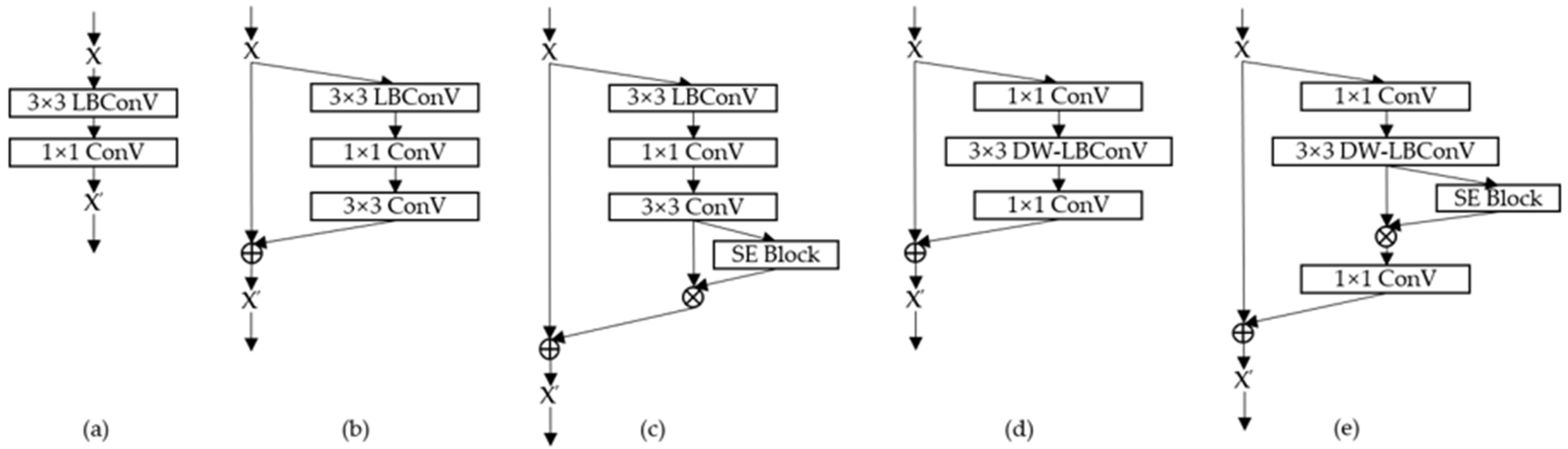
3.1. Depthwise LBC Layer and LB Mobile Inverted Bottleneck Block

Figure 2 showing the difference between the standard LBC and the LBC blocks we proposed. Figure 2a shows the structure of the LBCNN proposed in [41]; each LBC block is composed of two parts. The first part is a sparse LBC layer with non-trainable parameters. The structure of this layer is the same as the standard convolutional layer; the convolution kernel size is set to 3 × 3 without backpropagation. The parameters of the LBC kernel are to first generate a set of all-zero matrices and then replace a part of 0 randomly with 1 or −1 according to the Bernoulli distribution to generate a sparse LBC kernel. The second part is a standard convolution layer; the size of the convolution kernel is 1 × 1. In such an LBC block, it consists of a non-trainable convolutional layer and a trainable convolutional layer, so that the model can be trained normally. The 1 × 1 convolutional layer in the second part only provides a parameter that can be trained for the previous LBC layer. Figure 2b shows the structure of the standard LBC block with the residual module. The residual module adds shortcut connections, but does not change the structure of the LBC block. Figure 2c shows the structure of the standard LBC block with the SE-residual module.

In our work, we used depthwise convolution to construct the LBC layer. Compared with the standard LBC layer, the depth-separable LBC not only reduces the parameters, but also corresponds to each input feature map; there is only a 3 × 3 sparse LBC kernel for feature extraction, making the LBC kernel more intuitively reflect the result of its feature extraction shown as Figure 2d. At the same time, we introduced SE optimization to add attention weights to the feature maps extracted from the depthwise LBC layer, and used SE optimization weights to replace the 1 × 1 convolution of the traditional LBC layer shown in Figure 2e. In the entire mobile inverted bottleneck, the first and last two 1 × 1 convolutional layers are mainly used to adjust the number of input and output model channels. Even if we change the number of LBC kernels through model pruning, the input kernel output of the whole block will not change, which is convenient for the model to calculate the residual.

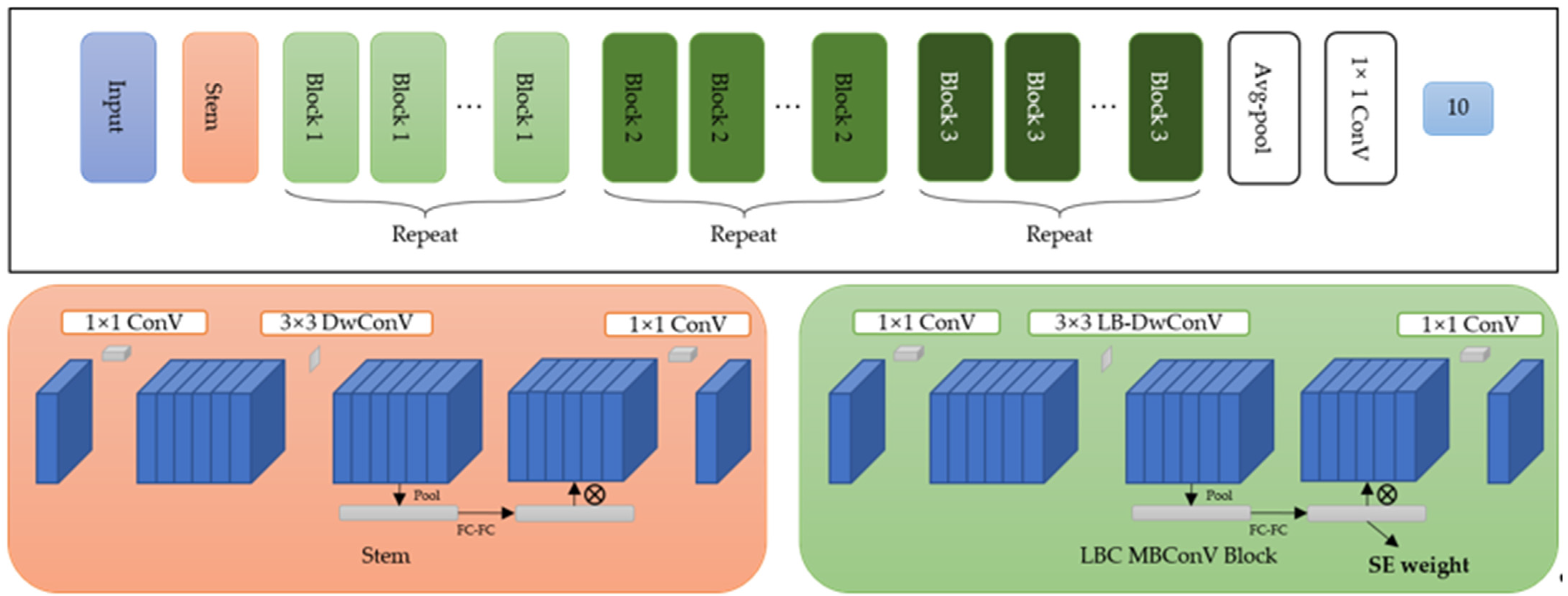
3.2. Baseline LB-MBNet Model

By combining the LBC mobile inverted bottleneck block, we propose our baseline model. The mobile inverted bottleneck has applications in many model structures and has also been proven to be an efficient model structure. In the EfficientNet [12], the input resolution, depth, and width of the model are all quantified, and an optimization search is performed to find the best performance model structure under different parameters. In our proposed model, the network width is also quantified, but we only change the number of LBC kernels in the depthwise LBC layer of each block. In the input of the model, we added a stem block to perform the first step of processing the input image. In this step, we used the standard convolutional layer instead of the LBC layer. In the subsequent model pruning, we do not prune the stem part, only pruning the block that uses the LBC. The expansion rate r in the model, that is, the ratio of the number of input channels in this block to the LBC convolution kernels in the block can be individually adjusted to adapt to different pruning scales. Figure 3 shows the proposed baseline model structure.

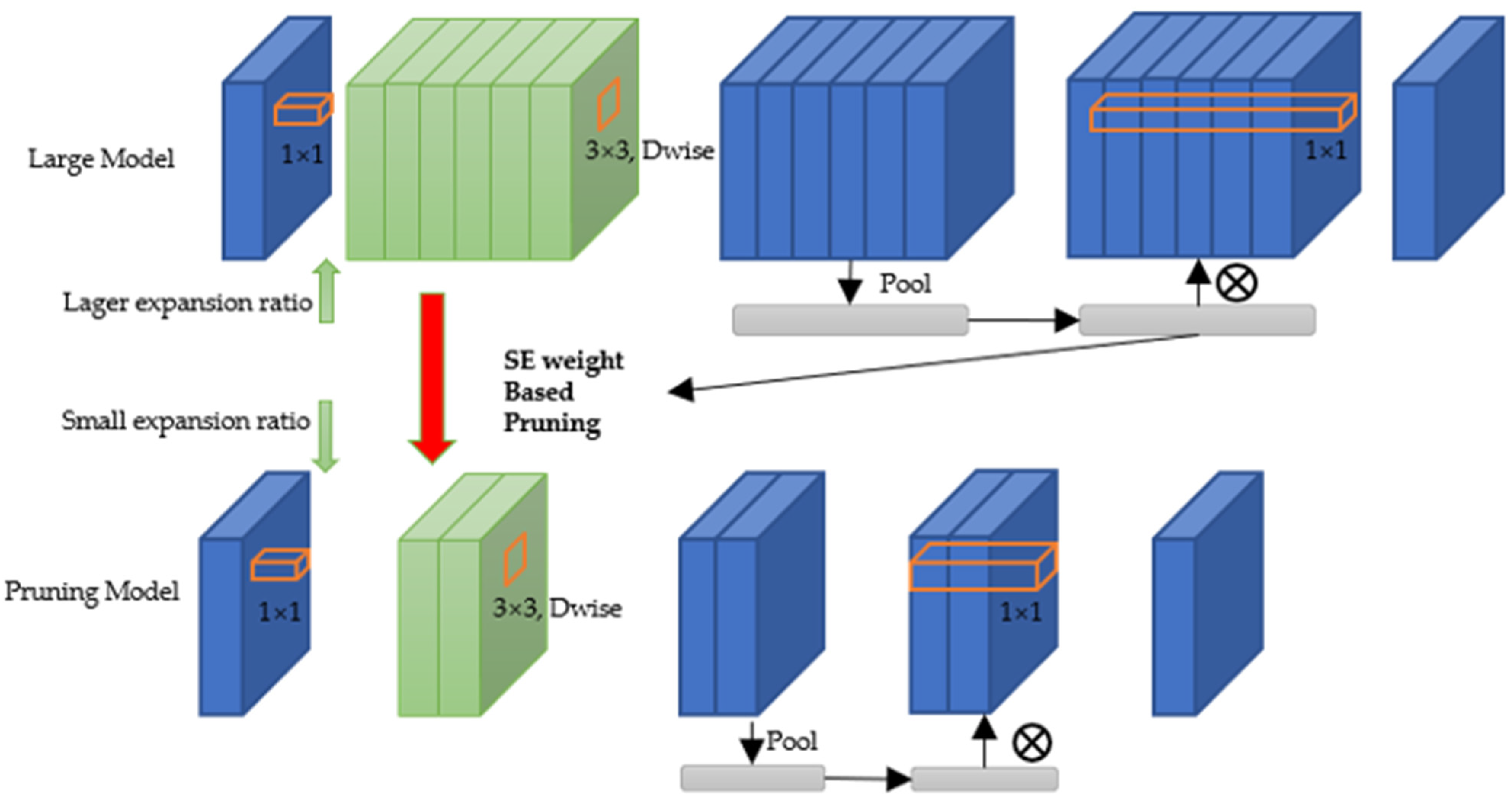
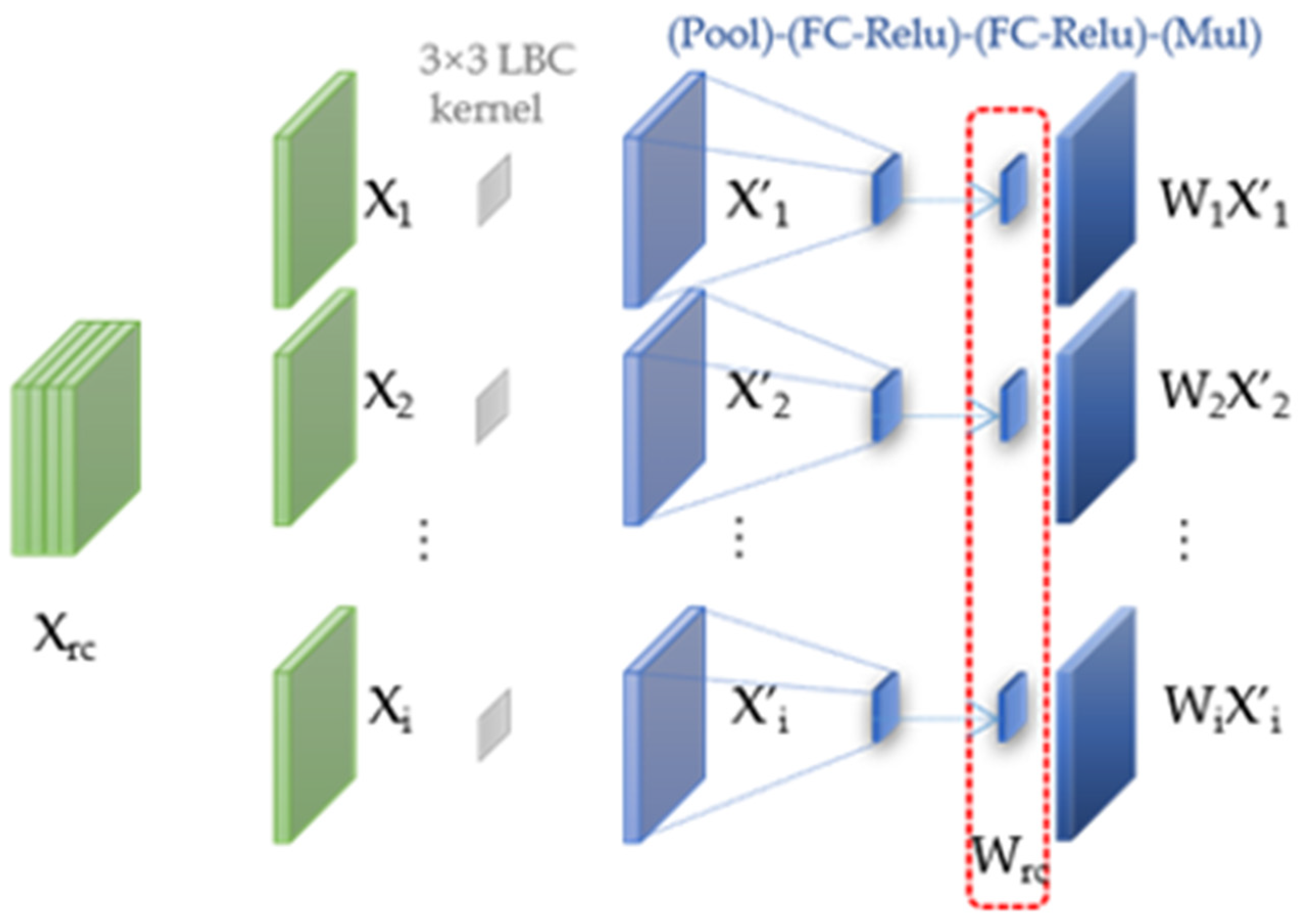
3.3. Model Pruning Based on SE Optimization Weight

As mentioned earlier in this paper, we directly connect the SE block and the depthwise LBC layer and use the SE optimization weight to express the importance of the LBC kernels. By setting the expansion rate r to a larger value, we can get a large model with more parameters. Through experiments on the database, we compared the accuracy performance of the large model and the small model and concluded that the results of the large model have better performance. This is also the basis for our model pruning.

SE optimization is used to perform global average pooling on the feature map of each channel and quantify the relative strength relationship between the features. It optimizes the attention weight of features in different feature channels for each sample. Corresponding to different samples, SE optimization weights are also different. However, we can calculate the mean value and distribution of SE optimization weights in large-scale samples, and score the characteristic channels in disguised form. Figure 4 shows the relationship between each LBC kernel and SE optimization weight in the proposed model. For the input X_c, c is the number of input feature channels. First, channel expansion is performed through 1 × 1 convolution to obtain X_rc. X_i (i ∈ 0…rc) is the i-th feature map in X_rc and X’_i is the output of the depthwise LBC layer. After the processing of the SE block, W_i (i ∈ 0…rc) is obtained.

For each sample, W_rc is the weight of this sample for each feature channel, and it is also the weight of the corresponding depthwise LBC kernel. By extracting the SE optimization weights of the overall sample of the database, we can count the mean and distribution of the SE optimization weights. Figure 5 shows the statistics of SE optimization weights of the training set on the CIFAR-10 database. Figure 5a shows our baseline model, using randomly initialized model parameters. Figure 5b shows a large model we built with more parameters by changing r. The parameters of (a) and (b) are initialized randomly, and the ratio of the model parameters is roughly equal to the ratio of the expansion ratio r. Figure 5c shows the use of the model pruning method we proposed. After pruning some of the convolution channels of model (b), (a) and (c) have the same expansion ratio and parameter amount. The parameters of (c) are calculated from (b).

In most of the blocks of (b), the number of SE optimization weights is large, the SE optimization with higher weights only accounts for a small part of the overall channel number, and many weights are close to 0. This also means that the LBC kernel corresponding to the channels with lower weight cannot extract significant features well in the entire data set. By filtering the SE optimization weights, we can get better LBC kernel parameters, each of which is a 3 × 3 sparse matrix. After model pruning, the SE weight distribution of the reconstructed model (c) is more concentrated than that of (a), and the LBC kernel has similar importance.

4. Experiment

4.1. Experiment Settings

For our proposed method, we use the CIFAR-10 database for image classification experiments. CIFAR-10 [45] is an image classification dataset containing a training set of 50K and a testing set of 10K 32 × 32 color images across the following 10 classes: airplanes, automobiles, birds, cats, deers, dogs, frogs, horses, ships, and trucks. Basically, all image classification models will be verified in the CIFAR-10 database.

In our test models, the model depth is fixed. In addition to the stem part, there are 4 MB blocks with LBC. Except for block 0, each block is repeated six times, and the scale of the feature map is halved in the initial layer of each block. Out of the SE blocks, each model has 59 convolutional layers, and there are 18 sets of SE optimization weights involving LBC in the last three blocks to participate in model pruning. Specific parameters are shown in

Table 1. Proposed baseline LB-MBNet-59 model structure and input resolution and output channel number of each stack. The repeat numbers in symbols are the parameters of the LB-MBNet-32 model.

Stack	Operator	Resolution	Channel	Repeat Num	Expansion Ratio
Stem	Conv3 × 3	32 × 32	32	1	-
0	LB-MBConv, k3 × 3	32 × 32	16	1	1
1	LB-MBConv, k3 × 3	32 × 32	64	6 (3)	6
2	LB-MBConv, k3 × 3	16 × 16	128	6 (3)	6
3	LB-MBConv, k3 × 3	8 × 8	256	6 (3)	6
Top	Conv1 × 1 and Pooling and FC	4 × 4	512	1	-

. Besides, we also set the number of repetitions of each block to 3 and established a model of 32 convolutional layers.

For the input data, we use data augmentation to expand the training data. The operations include width shift, height shift, and horizontal flip; the shift range is 4 pixels. All models are compiled using the stochastic gradient descent (SGD) method; the initial learning rate is set to 0.1, and decays by 0.1 at 80, 140, and 180 epochs. Each model is first trained for 200 epochs and then pruned, and then trained again for 200 epochs using the same hyperparameters. We use a graphics card “NVIDIA TITAN X Pascal” as the hardware for our experiments. The GPU operates at a frequency of 1417 MHz.

4.2. Experimental Result

In this chapter, we will evaluate the effect of the LBC layer in the proposed baseline model and compare its performance to that of the standard convolutional layer. At the same time, by changing the value of the expansion ratio r, the impact of different model scales on the recognition results is evaluated.

Table 2. Model recognition result with different expansion ratio r.

Model Name	Accuracy Rate (%)	Trainable Params	FLOPs (108)	Ratio to r6 Model
LB-MBNet-59-r6	92.47	7.11 M	4.57	1×
LB-MBNet-59-r10	93.65	11.75 M	7.57	1.7×
LB-MBNet-59-r18	93.81	21.03 M	13.6	3.0×
LB-MBNet-59-r30	94.40	34.96 M	22.5	4.9×
LB-MBNet-59-r60	95.05	69.78 M	45.0	9.8×
LB-MBNet-59-r80	96.06	92.99 M	59.9	13.1×
LB-MBNet-32-r6	92.88	3.19 M	2.16	1×
LB-MBNet-32-r80	95.63	40.84 M	27.7	12.8×

shows the model recognition result obtained while adjusting the expansion ratio r. We calculated the parameters and floating-point operations per second (FLOPS) of the model.

From Table 2, we can conclude that, with the increase in r, the trainable parameter amount and FLOPs of the model also increase almost linearly. The accuracy of the model has also increased. When r = 6, the recognition accuracy of the LB-MBNet-59-r6 model reached 92.47%, whereas that of the LB-MBNet-32-r6 model reached 92.88%. When r = 80, the recognition accuracy of the LB-MBNet-59-r80 model reached 96.06%, whereas that of the LB-MBNet-32-r80 model reached 95.63%, increasing by 3.59% and 2.75%, respectively.

For the experiment of model pruning, we use the model with the best results and the maximum number of parameters as the basic model and obtain the mean value of SE optimization weight through 50 K samples of the training data set. For different optimization scales, we only keep the part with the larger SE optimization weight value and pruning the corresponding layers in each block of the model. In our experiment, we separately prune the model in segmented and one-shot ways. In the segmented experiment, the r-value will gradually drop to the optimal scale we expect. In the one-shot experiment, we use the basic model to directly modify the r-value to the optimal scale we expect.

Table 3. Model recognition result with rebuilt model from r80 model.

Model Name	Accuracy Rate (%)	Trainable Params	FLOPs (108)	Ratio to r6 Model
LB-MBNet-59-r80	96.06	92.99 M	59.9	13.1×
Re-LB-MBNet-59-r40	96.15	46.57 M	30.0	6.6×
Re-LB-MBNet-59-r20	95.76	23.36 M	15.0	3.3×
Re-LB-MBNet-59-r18	95.58	21.03 M	13.6	3.0×
Re-LB-MBNet-59-r10	95.65	11.75 M	7.57	1.7×
Re-LB-MBNet-59-r6	95.24	7.11 M	4.57	1×
Re-LB-MBNet-59-r3	93.97	3.63 M	2.33	0.5×
LB-MBNet-32-r80	95.63	40.84 M	27.7	12.8×
Re-LB-MBNet-32-r6	94.90	3.19 M	2.16	1×

showing the result of model pruning. We use the r80 model as the basic model for one-shot pruning. Here, we transfer the weight of the corresponding part to the rebuilt model according to the fixed r.

From Table 3, we can conclude that, after the model is pruned, the accuracy rate remains at a relatively high level.

In the LB-MBNet-59 model, compared with the basic r80 model, the accuracy of the r40 model reaches 96.15%, which is an improvement of 0.09% on the basic model. We believe this is because the parameters of the r80 model are relatively high, and the model has over-fitting. In the case of reducing half of parameters while maintaining a more effective LBC kernel, the results of the r40 model have risen slightly. As we continue to reduce the expansion ratio, although the accuracy of the model has dropped slightly, compared with the randomly initialized model, the results of the pruning-rebuild model are significantly better. When the expansion ratio r is reduced to 6, the model parameters and FLOPs return to the level of the basic r6 model we proposed, but the rebuilt model result has been improved by 2.77% to 95.24%. At the same time, compared with the r80 model at the beginning of pruning, the accuracy rate is only reduced by 0.82%, and the parameter amount and FLOPs are reduced by 92% of the r80 model. This result proves that our proposed method is effective.

We further reduced the expansion ratio to r3. At this time, the Re-LB-MBNet-59-r3 model accuracy rate dropped significantly, reaching 93.97%, which is a 1.27% drop compared with the r6 model. However, compared with the randomly initialized r6 model, the parameters and FLOPs of this result decreased by 50%, but the result increased by 1.50%. We think that, because the expansion ratio is too small, the generalization ability of the model is not enough, which leads to overfitting at 93.97%. However, because the LBC kernel is not trainable, and after selection through model pruning, the result is better than random initialization.

In the LB-MBNet-32 model, the accuracy of the rebuilt Re-LB-MBNet-32-r6 model reaches 94.90%. Compared with the LB-MBNet-32-r80 model, it has only decreased by 0.73%. However, compared with the basic LB-MBNet-32-r6 model, it has increased by 2.02%. The resulting level of LB-MBNet-59-r3 and LB-MBNet-32-r6 is similar, but the latter has fewer parameters and FLOPs.

4.3. Comparison with State-of-the-Art

We also compared the results of our proposed method with the state-of-the-art methods. At the same time, because many model pruning methods use ResNetV2-56 [63] as the basic model on the CIFAR-10 database, the baseline model we proposed has a similar number of convolutional layers (59 layers). We also compared the model pruning method based on ResNetV2-56. However, it should be noted that, because we have applied the SE optimization part in the proposed model, the amount of model parameters has also increased.

Table 4. Comparison results with the state-of-the-art methods on the CIFAR-10 database. FLOPS, floating-point operations per second.

Methods	Accuracy Rate (%)	Params (M)	Params Pruned (%)	FLOPs (108)	FLOPs Pruned (%)
ResNetV2-56 1 [63]	93.01	0.597	-	1.71	-
Li et al. [20]	93.03	0.516	13.7	1.24	27.6
NISP [64]	92.98	0.343	42.6	0.96	43.6
DCP-A [64]	93.02	0.177	70.3	0.90	47.1
CP [51]	92.01	0.597	0	0.86	50.0
AMC [65]	92.11	0.597	0	0.86	50.0
C-SGD [31]	93.24	0.597	0	0.67	60.8
GBN-40 [66]	93.34	0.278	53.5	0.68	60.1
ResNetV2-164 1 [63]	94.58	1.73	-	4.97	-
L1-Sparse [52]	94.92	1.44	16.8	3.81	23.3
ResNetV2-1001 [63]	95.08	10.48	-	30.3	-
MobileNetV2 1 [43]	91.93	2.2	-	0.88	-
AutoSlim [67]	93.20	1.5	31.8	0.88	0
MobileNetV3 [50]	92.97	1.52	-	0.35	-
LB-MBNet-59-r6 1	92.35	7.11	-	4.57	-
Re-LB-MBNet-59-r6	95.24	7.11	0	4.57	0
Re-LB-MBNet-59-r3	93.97	3.63	48.9	2.33	49
LB-MBNet-32-r6 1	92.88	3.19	-	2.16	-
Re-LB-MBNet-32-r6	94.90	3.19	0	2.16	0

¹ Baseline model of model pruning.

shows the comparison results between our proposed method and the state-of-the-art methods.

Table 4 shows that the results of our method obtained relatively better accuracy compared with the state-of-the-art methods. Because our model uses the SE optimization module, our model has a relatively large number of parameters. However, because the convolution kernel with a size of 1 × 1 is also used in the SE optimization module, the increase in the number of parameters has little effect on the amount of calculation. Through the results of the two baseline models of LB-MBNet-59-r6 and LB-MBNet-32-r6, the recognition accuracy is not good. However, after the expansion and pruning operation, the recognition accuracy of Re-LB-MBNet-59-r6 has reached the state-of-the-art level while keeping the number of model parameters and calculations unchanged. Among the Re-LB-MBNet-59-r6 models, the most similar result is the ResNetV2-1001 [63] model, but our mode has much fewer parameters, and the FLOPs are only about 15%. Besides, in the Re-LB-MBNet-32-r6 model, the ResNetV2-164 [63] and L1-Sparse [52] models are the closest results. Although our models have more model parameters, but fewer FLOPs.

In our proposed method, precisely through SE optimization weights to score and prune the LBC kernel, we can make full use of the advantages of the untrainable kernel to obtain a model with less computation and high accuracy. Based on [29], the weight of the network after pruning by other methods is not very important, and our method truly retained only better model parameters.

4.4. Discussion

As we envisioned, the method of superimposing the non-trainable layer and the trainable layer can reduce the training parameters while allowing the model to be normally constructed into an end-to-end structure. However, the initialization of the non-trainable layer is very important. All parameters in the standard convolutional network can be trained, and reasonable parameters can be found through the optimization method of the model. However, in a convolution model with non-trainable parameters, it is necessary to filter out reasonable parameters through the methods like model pruning. In our proposed method, not only the advantages of LBC are maintained, which has a sparse and non-trainable binary convolution kernel, and at the same time, more reasonable LBC parameters are found through the method of model pruning, and the model with high recognition accuracy and fewer model parameters is obtained.

Besides, the proposed method uses data-driven SE optimization weights as the evaluation of pruning, and the results are obtained based on the results of model training, which are more accurate than some manually designed evaluation indicators. The basic model we proposed can evolve towards faster and more miniaturization. It is necessary to further optimize the depth and width of the model. However, this has already involved the research field of NAS and has not been carried out in this paper. The experimental results have been able to prove the effectiveness of our current proposed method.

5. Conclusions

Inspired by LBC and SE optimization, we propose a depthwise LBC and SE optimization model structure in this paper. By increasing the expansion ratio of the inverse bottleneck structure in the model, a large model with higher accuracy, but a huge number of parameters can be obtained through training. AccordFing to the SE optimization weight, we perform channel-based model pruning of the basic model and only retain the depthwise LBC convolution channel that contributes more to the result. Our experimental results of image classification on the CIFAR-10 database prove the effectiveness of our proposed method. Our proposed method shows that the untrainable convolution kernel has the same feature expression capabilities as standard CNNs, and through pruning based on SE weights, it can indeed retain the more powerful untrainable convolution kernels from the large model.

References

1. Zhuang, Z.; Tan, M.; Zhuang, B.; Liu, J.; Guo, Y.; Wu, Q.; Huang, J.; Zhu, J. Discrimination-aware channel pruning for deep neural networks. arXiv 2018, arXiv:1810.11809. [Google Scholar]
2. Ding, X.; Ding, G.; Guo, Y.; Han, J. Centripetal sgd for pruning very deep convolutional networks with complicated structure. In Proceedings of the IEEE/CVF Conference on Computer Vision and Pattern Recognition, Long Beach, CA, USA, 16–20 June 2019; pp. 4943–4953. [Google Scholar]
3. Simonyan, K.; Zisserman, A. Very deep convolutional networks for large-scale image recognition. arXiv 2014, arXiv:1409.1556. [Google Scholar]
4. Denton, E.; Zaremba, W.; Bruna, J.; LeCun, Y.; Fergus, R. Exploiting linear structure within convolutional networks for efficient evaluation. arXiv 2014, arXiv:1404.0736. [Google Scholar]
5. Szegedy, C.; Vanhoucke, V.; Ioffe, S.; Shlens, J.; Wojna, Z. Rethinking the inception architecture for computer vision. In Proceedings of the IEEE Conference on Computer Vision and Pattern Recognition, Las Vegas, NV, USA, 26 June–1 July 2016; pp. 2818–2826. [Google Scholar]
6. Szegedy, C.; Ioffe, S.; Vanhoucke, V.; Alemi, A. Inception-v4, inception-resnet and the impact of residual connections on learning. In Proceedings of the AAAI Conference on Artificial Intelligence, San Francisco, CA, USA, 4–9 February 2017. [Google Scholar]
7. He, K.; Zhang, X.; Ren, S.; Sun, J. Deep residual learning for image recognition. In Proceedings of the IEEE Conference on Computer Vision and Pattern Recognition, Las Vegas, NV, USA, 26 June–1 July 2016; pp. 770–778. [Google Scholar]
8. Iandola, F.N.; Han, S.; Moskewicz, M.W.; Ashraf, K.; Dally, W.J.; Keutzer, K. SqueezeNet: AlexNet-level accuracy with 50x fewer parameters and <0.5 MB model size. arXiv 2016, arXiv:1602.07360. [Google Scholar]
9. Wu, J.; Leng, C.; Wang, Y.; Hu, Q.; Cheng, J. Quantized convolutional neural networks for mobile devices. In Proceedings of the IEEE Conference on Computer Vision and Pattern Recognition, Las Vegas, NV, USA, 26 June–1 July 2016; pp. 4820–4828. [Google Scholar]
10. Howard, A.G.; Zhu, M.; Chen, B.; Kalenichenko, D.; Wang, W.; Weyand, T.; Andreetto, M.; Adam, H. Mobilenets: Efficient convolutional neural networks for mobile vision applications. arXiv 2017, arXiv:1704.04861. [Google Scholar]
11. Liu, W.; Anguelov, D.; Erhan, D.; Szegedy, C.; Reed, S.; Fu, C.Y.; Berg, A.C. SSD: Single shot multibox detector. In European Conference on Computer Vision; Springer: Cham, Switzerland, 2016; pp. 21–37. [Google Scholar]
12. Tan, M.; Le, Q. Efficientnet: Rethinking model scaling for convolutional neural networks. In Proceedings of the International Conference on Machine Learning. ICML, Long Beach, CA, USA, 9–15 June 2019; pp. 6105–6114. [Google Scholar]
13. Cao, X.; Li, T.; Li, H.; Xia, S.; Ren, F.; Sun, Y.; Xu, X. A robust parameter-free thresholding method for image segmentation. IEEE Access 2018, 7, 3448–3458. [Google Scholar] [CrossRef]
14. Jaderberg, M.; Vedaldi, A.; Zisserman, A. Speeding up convolutional neural networks with low rank expansions. arXiv 2014, arXiv:1405.3866. [Google Scholar]
15. Hinton, G.; Vinyals, O.; Dean, J. Distilling the knowledge in a neural network. arXiv 2015, arXiv:1503.02531. [Google Scholar]
16. Jacob, B.; Kligys, S.; Chen, B.; Zhu, M.; Tang, M.; Howard, A.; Adam, H.; Kalenichenko, D. Quantization and training of neural networks for efficient integer-arithmetic-only inference. In Proceedings of the IEEE Conference on Computer Vision and Pattern Recognition, Salt Lake City, UT, USA, 18–22 June 2018; pp. 2704–2713. [Google Scholar]
17. Krishnamoorthi, R. Quantizing deep convolutional networks for efficient inference: A whitepaper. arXiv 2018, arXiv:1806.08342. [Google Scholar]
18. LeCun, Y.; Denker, J.S.; Solla, S.A.; Howard, R.E.; Jackel, L.D. Optimal brain damage. In Proceedings of the Advances in Neural Information Processing Systems, Denver, CO, USA, 27–30 November 1989; Volume 2, pp. 598–605. [Google Scholar]
19. Hassibi, B.; Stork, D.G. Second Order Derivatives for Network Pruning: Optimal Brain Surgeon; Morgan Kaufmann: Denver, CO, USA, 1993; pp. 164–171. [Google Scholar]
20. Li, H.; Kadav, A.; Durdanovic, I.; Samet, H.; Graf, H.P. Pruning filters for efficient convnets. arXiv 2016, arXiv:1608.08710. [Google Scholar]
21. Zhu, M.; Gupta, S. To prune, or not to prune: Exploring the efficacy of pruning for model compression. arXiv 2017, arXiv:1710.01878. [Google Scholar]
22. Luo, J.H.; Wu, J.; Lin, W. Thinet: A filter level pruning method for deep neural network compression. In Proceedings of the IEEE International Conference on Computer Vision, Honolulu, HI, USA, 21–26 July 2017; pp. 5058–5066. [Google Scholar]
23. Carreira-Perpinán, M.A.; Idelbayev, Y. “learning-compression” algorithms for neural net pruning. In Proceedings of the IEEE Conference on Computer Vision and Pattern Recognition, Salt Lake City, UT, USA, 18–22 June 2018; pp. 8532–8541. [Google Scholar]
24. Han, S.; Pool, J.; Tran, J.; Dally, W.J. Learning both weights and connections for efficient neural networks. arXiv 2015, arXiv:1506.02626. [Google Scholar]
25. Louizos, C.; Welling, M.; Kingma, D.P. Learning Sparse Neural Networks through L0 Regularization. arXiv 2017, arXiv:1712.01312. [Google Scholar]
26. Huang, Z.; Wang, N. Data-driven sparse structure selection for deep neural networks. In Proceedings of the European Conference on Computer Vision (ECCV), Munich, Germany, 8–14 September 2018; pp. 304–320. [Google Scholar]
27. Chin, T.W.; Zhang, C.; Marculescu, D. Layer-compensated pruning for resource-constrained convolutional neural networks. arXiv 2018, arXiv:1810.00518. [Google Scholar]
28. Han, S.; Liu, X.; Mao, H.; Pu, J.; Pedram, A.; Horowitz, M.A.; Dally, W.J. EIE: Efficient inference engine on compressed deep neural network. ACM Sigarch Comput. Archit. News 2016, 44, 243–254. [Google Scholar] [CrossRef]
29. Liu, Z.; Sun, M.; Zhou, T.; Huang, G.; Darrell, T. Rethinking the value of network pruning. arXiv 2018, arXiv:1810.05270. [Google Scholar]
30. Elsken, T.; Metzen, J.H.; Hutter, F. Neural architecture search: A survey. J. Mach. Learn. Res. 2019, 20, 1–21. [Google Scholar]
31. Itti, L.; Koch, C.; Niebur, E. A model of saliency-based visual attention for rapid scene analysis. IEEE Trans. Pattern Anal. Mach. Intell. 1998, 20, 1254–1259. [Google Scholar] [CrossRef] [Green Version]
32. Corbetta, M.; Shulman, G.L. Control of goal-directed and stimulus-driven attention in the brain. Nat. Rev. Neurosci. 2002, 3, 201–215. [Google Scholar] [CrossRef] [PubMed]
33. Jaderberg, M.; Simonyan, K.; Zisserman, A.; Kavukcuoglu, K. Spatial transformer networks. arXiv 2015, arXiv:1506.02025. [Google Scholar]
34. Bhowmik, P.; Pantho, M.J.H.; Bobda, C. HARP: Hierarchical Attention Oriented Region-Based Processing for High-Performance Computation in Vision Sensor. Sensors 2021, 21, 1757. [Google Scholar] [CrossRef] [PubMed]
35. Bhowmik, P.; Pantho, M.J.H.; Bobda, C. Bio-inspired smart vision sensor: Toward a reconfigurable hardware modeling of the hierarchical processing in the brain. J. Real-Time Image Process. 2020, 18, 157–174. [Google Scholar] [CrossRef]
36. Wang, X.; Girshick, R.; Gupta, A.; He, K. Non-local neural networks. In Proceedings of the IEEE Conference on Computer Vision and Pattern Recognition, Salt Lake City, UT, USA, 18–22 June 2018; pp. 7794–7803. [Google Scholar]
37. Hu, J.; Shen, L.; Sun, G. Squeeze-and-excitation networks. In Proceedings of the IEEE Conference on Computer Vision and Pattern Recognition, Salt Lake City, UT, USA, 18–22 June 2018; pp. 7132–7141. [Google Scholar]
38. Woo, S.; Park, J.; Lee, J.Y.; Kweon, I.S. Cbam: Convolutional block attention module. In Proceedings of the European Conference on Computer Vision (ECCV), Munich, Germany, 8–14 September 2018; pp. 3–19. [Google Scholar]
39. Cao, Y.; Xu, J.; Lin, S.; Wei, F.; Hu, H. Gcnet: Non-local networks meet squeeze-excitation networks and beyond. In Proceedings of the IEEE/CVF International Conference on Computer Vision Workshops, Long Beach, CA, USA, 16–20 June 2019. [Google Scholar]
40. Liu, W.; Wu, G.; Ren, F.; Kang, X. DFF-ResNet: An insect pest recognition model based on residual networks. Big Data Min. Anal. 2020, 3, 300–310. [Google Scholar] [CrossRef]
41. Juefei-Xu, F.; Naresh Boddeti, V.; Savvides, M. Local binary convolutional neural networks. In Proceedings of the IEEE Conference on Computer Vision and Pattern Recognition, Honolulu, HI, USA, 21–26 July 2017; pp. 19–28. [Google Scholar]
42. Ojala, T.; Pietikainen, M.; Harwood, D. Performance evaluation of texture measures with classification based on Kullback discrimination of distributions. In Proceedings of the 12th International Conference on Pattern Recognition, Jerusalem, Israel, 9–13 October 1994; Volume 1, pp. 582–585. [Google Scholar]
43. Sandler, M.; Howard, A.; Zhu, M.; Zhmoginov, A.; Chen, L.C. Mobilenetv2: Inverted residuals and linear bottlenecks. In Proceedings of the IEEE Conference on Computer Vision and Pattern Recognition, Salt Lake City, UT, USA, 18–22 June 2018; pp. 4510–4520. [Google Scholar]
44. Howard, A.; Sandler, M.; Chu, G.; Chen, L.C.; Chen, B.; Tan, M.; Wang, W.; Zhu, Y.; Pang, R.; Vasudevan, V.; et al. Searching for mobilenetv3. In Proceedings of the IEEE/CVF International Conference on Computer Vision, Seoul, Korea, 27 October–2 November 2019; pp. 1314–1324. [Google Scholar]
45. Krizhevsky, A.; Hinton, G. Learning Multiple Layers of Features from Tiny Images; Citeseer: University Park, PA, USA, 2009. [Google Scholar]
46. Rakhuba, M.; Oseledets, I.; Lempitsky, V.; Lebedev, V.; Ganin, Y. Speeding-up convolutional neural networks using fine-tuned cp-decomposition. arXiv 2018, arXiv:1412.6553. [Google Scholar]
47. Courbariaux, M.; Hubara, I.; Soudry, D.; El-Yaniv, R.; Bengio, Y. Binarized neural networks: Training deep neural networks with weights and activations constrained to+ 1 or-1. arXiv 2016, arXiv:1602.02830. [Google Scholar]
48. Rastegari, M.; Ordonez, V.; Redmon, J.; Farhadi, A. Xnor-net: Imagenet classification using binary convolutional neural networks. In European Conference on Computer Vision; Springer: Cham, Switzerland, October 2016; pp. 525–542. [Google Scholar]
49. Romero, A.; Ballas, N.; Kahou, S.E.; Chassang, A.; Gatta, C.; Bengio, Y. Fitnets: Hints for thin deep nets. arXiv 2014, arXiv:1412.6550. [Google Scholar]
50. Molchanov, D.; Ashukha, A.; Vetrov, D. Variational dropout sparsifies deep neural networks. In Proceedings of the International Conference on Machine Learning, ICML, Sydney, Australia, 6–11 August 2017; pp. 2498–2507. [Google Scholar]
51. He, Y.; Zhang, X.; Sun, J. Channel pruning for accelerating very deep neural networks. In Proceedings of the IEEE International Conference on Computer Vision, Honolulu, HI, USA, 21–26 July 2017; pp. 1389–1397. [Google Scholar]
52. Liu, Z.; Li, J.; Shen, Z.; Huang, G.; Yan, S.; Zhang, C. Learning efficient convolutional networks through network slimming. In Proceedings of the IEEE International Conference on Computer Vision, Honolulu, Hawaii, USA, 21–26 July 2017; pp. 2736–2744. [Google Scholar]
53. Hu, M.; Qian, F.; Guo, D.; Wang, X.; He, L.; Ren, F. ETA-rPPGNet: Effective Time-Domain Attention Network for Remote Heart Rate Measurement. IEEE Trans. Instrum. Meas. 2021, 70, 1–12. [Google Scholar]
54. Zhang, G.; Huang, X.; Li, S.Z.; Wang, Y.; Wu, X. Boosting local binary pattern (LBP)-based face recognition. In Chinese Conference on Biometric Recognition; Springer: Berlin/Heidelberg, Germany, December 2004; pp. 179–186. [Google Scholar]
55. Hu, M.; Yang, C.; Zheng, Y.; Wang, X.; He, L.; Ren, F. Facial Expression Recognition Based on Fusion Features of Center-Symmetric Local Signal Magnitude Pattern. IEEE Access 2019, 7, 118435–118445. [Google Scholar] [CrossRef]
56. Nanni, L.; Lumini, A.; Brahnam, S. Survey on LBP based texture descriptors for image classification. Expert Syst. Appl. 2012, 39, 3634–3641. [Google Scholar] [CrossRef]
57. Courbariaux, M.; Bengio, Y.; David, J.P. Binaryconnect: Training deep neural networks with binary weights during propagations. arXiv 2015, arXiv:1511.00363. [Google Scholar]
58. Sifre, L.; Mallat, S. Rigid-motion scattering for texture classification. arXiv 2014, arXiv:1403.1687. [Google Scholar]
59. Chollet, F. Xception: Deep learning with depthwise separable convolutions. In Proceedings of the IEEE Conference on Computer Vision and Pattern Recognition, Honolulu, HI, USA, 21–26 July 2017; pp. 1251–1258. [Google Scholar]
60. Krizhevsky, A.; Sutskever, I.; Hinton, G.E. Imagenet classification with deep convolutional neural networks. Adv. Neural Inf. Process. Syst. 2012, 25, 1097–1105. [Google Scholar] [CrossRef]
61. Xie, S.; Girshick, R.; Dollár, P.; Tu, Z.; He, K. Aggregated residual transformations for deep neural networks. In Proceedings of the IEEE Conference on Computer Vision and Pattern Recognition, Honolulu, HI, USA, 21–26 July 2017; pp. 1492–1500. [Google Scholar]
62. Kumawat, S.; Verma, M.; Raman, S. LBVCNN: Local binary volume convolutional neural network for facial expression recognition from image sequences. In Proceedings of the IEEE/CVF Conference on Computer Vision and Pattern Recognition Workshops, Long Beach, CA, USA, 16–20 June 2019. [Google Scholar]
63. He, K.; Zhang, X.; Ren, S.; Sun, J. Identity mappings in deep residual networks. In European Conference on Computer Vision; Springer: Cham, Switzerland, October 2016; pp. 630–645. [Google Scholar]
64. Yu, R.; Li, A.; Chen, C.F.; Lai, J.H.; Morariu, V.I.; Han, X.; Gao, M.; Lin, C.Y.; Davis, L.S. Nisp: Pruning networks using neuron importance score propagation. In Proceedings of the IEEE Conference on Computer Vision and Pattern Recognition, Salt Lake City, UT, USA, 18–22 June 2018; pp. 9194–9203. [Google Scholar]
65. He, Y.; Lin, J.; Liu, Z.; Wang, H.; Li, L.J.; Han, S. Amc: Automl for model compression and acceleration on mobile devices. In Proceedings of the European Conference on Computer Vision (ECCV), Munich, Germany, 8–14 September 2018; pp. 784–800. [Google Scholar]
66. You, Z.; Yan, K.; Ye, J.; Ma, M.; Wang, P. Gate decorator: Global filter pruning method for accelerating deep convolutional neural networks. arXiv 2019, arXiv:1909.08174. [Google Scholar]
67. Yu, J.; Huang, T. Autoslim: Towards one-shot architecture search for channel numbers. arXiv 2019, arXiv:1903.11728. [Google Scholar]
Figure 1. The proposed model pruning method is based on SE (squeeze-and-excitation) optimization weight. Build a model with higher accuracy by setting a larger expansion ratio (above model). Calculate the SE weight of the corresponding part of the training data set, and score the depthwise convolution kernel. Cut the corresponding depthwise convolution kernel to get a smaller model (below model). The accuracy of the model remains at a similar level.
Electronics 10 01329 g001
Figure 2. The difference between the standard LBC (local binary convolution) and the LBC blocks we proposed. (a) standard LBC layer; (b) standard LBC with residual module; (c) standard LBC with SE-residual module; (d) standard depthwise LBC with mobile inverse bottleneck module; (e) standard depthwise LBC with SE-mobile inverse bottleneck module.
Electronics 10 01329 g002
Figure 3. The proposed baseline LB-MBNet model framework.
Electronics 10 01329 g003
Figure 4. Relationship between LBC kernel and SE weight; each weight corresponds to a 3 × 3 LBC kernel.
Electronics 10 01329 g004
Figure 5. The statistics of SE optimization weights of the training set on the CIFAR-10 database. (a) The model with the expansion ratio r = 6, random initialization; (b) the model with r = 80, random initialization; (c) the model with r = 6, pruning and retraining from the model r = 80. Each subfigure represents the three blocks in stack 1 of each model.
Electronics 10 01329 g005