A Novel Decomposition Model for Visual Rail Surface Inspection

Abstract

Rail surface inspection plays a pivotal role in large-scale railway construction and development. However, accurately identifying possible defects involving a large variety of visual appearances and their dynamic illuminations remains challenging. In this paper, we fully explore and use the essential attributes of our defect structure data and the inherent temporal and spatial characteristics of the track to establish a general theoretical framework for practical applications. As such, our framework can overcome the bottleneck associated with machine vision inspection technology in complex rail environments. In particular, we consider a differential regular term for background rather than a traditional low-rank constraint to ensure that the model can tolerate dynamic background changes without losing sensitivity when detecting defects. To better capture the compactness and completeness of a defect, we introduce a tree-shaped hierarchical structure of sparse induction norms to encode the spatial structure of the defect area. The proposed model is evaluated with respect to two newly released Type-I/II rail surfaces discrete defects (RSDD) data sets and a practical rail line. Qualitative and quantitative evaluations show that the decomposition model can handle the dynamics of the track surface well and that the model can be used for structural detection of the defect area.

1. Introduction

With progressively large-scale high-speed railway construction and increasingly rapid development, ensuring safe service is becoming ever more important. Practice shows that long-term repeated loads inevitably cause microscopic damage to railway facilities, deterioration of the main structural components, and reduction of infrastructure performance. Expanded operating hours result in frequent large-scale mass deterioration across a large number of lines. For example, some lines exhibit serious structural defects such as continuous fastener failure and broken rails because of their extreme operating environments. Generally speaking, railway defects are a sign of potentially serious safety hazards. Failure to deal with these defects promptly will shorten the service life of railway facilities and directly affect the safety of line operations. To make up for the shortcomings of existing detection methods, the development of intelligent detection technologies has become a requirement for maintaining the safe and stable operation of high-speed railway lines [1]. The traditional method of relying on manual inspection no longer meets the actual needs, and intelligent detection technology based on computer vision has attracted significant attention in recent years [2,3,4]. With the continuous development of related theories and technologies such as image processing, machine learning, and artificial intelligence, research in computer vision is gradually shifting from theory to practical applications, to newly proposed vision detection models for specific applications, and to the development of corresponding algorithms.

Visual inspection based on image processing and pattern recognition methods is a recently developed technology. It is considered one of the technologies with the highest potential in rail surface scratch detection [5,6]. In the visual inspection system, a high-speed (usually linear) camera is installed on an inspection train. The camera collects images of the track and uses computer vision and pattern recognition methods to detect defects in the track components. Surface defect detection is a relatively active field of application in current computer vision research. It has been widely used in industrial inspection, such as for textile contamination detection [7,8] and metal welding surface detection [9], among others.

Defect detection is generally divided into two stages, including image feature extraction and defect recognition. Mandriota et al. [10] first adopted Gabor transformation of an input image to form a feature vector. They then applied SVM to recognize scratched rails. Marino et al. [11] proposed a real-time track detection system based on wavelet transformation and multi-layer perception. Li et al. proposed a real-time discrete rail surface scratch detection method [12]. Firstly, the proposed system enhances contrast between defects and background using the local normalization (LN) method, which is nonlinear and illumination independent. Subsequently, the defect localization based on projection profile (DLBP) algorithm is presented to identify possible defects. Instead of LN+DLBP, MLC+PEME is proposed to investigate the possible discrete defects [13]. MLC (Local Michelson-like contrast) first enhances image contrast, and then PEME (proportion emphasized maximum entropy) automatically locates possible defects by maximizing the object entropy while keeping the defect proportion in low-level. He et al. [14] used a defect enhancement algorithm based on reverse Peronal–Malik (P–M) diffusion. In addition, some improvements have been proposed, such as the use of a cascaded learning form of weak classifiers [15] or the Latent Dirichlet Allocation (LDA) model [16] for fastener deterioration. This type of method generally achieves a better classification accuracy, but it cannot always be used to classify defects characterized by small or large intraclass differences. Alternatively, applications of deep learning have been developed rapidly, in terms of both detection accuracy and algorithm execution efficiency. On the basis of these widely used technologies, a number of methods have been proposed. For example, Gibert et al. [17] used deep convolutional neural networks (DCNNs) for automatic detection of fastener state and proved the method’s effectiveness. This type of method can generally achieve better recognition accuracy, but it is often associated with high training complexity and requires a large number of training samples to prevent overfitting.

In the field of track inspection, intrinsic variability of the imaging environment, the complex evolution of the line state, and the diversity, scale difference, and sparseness of weak defects in a railway system (such as track surface defects) pose severe challenges. Although track defect detection research has made considerable progress, it still faces three shortcomings, including robustness, generalization, and accuracy. Specifically, factors such as external lighting, camera shake, and noise in the operating environment can significantly affect system performance [5,7]. Many methods proposed in the literature are only effective for specific types of defect and lack a general defect detection model and theoretical framework [12,16]. In actual operations, the false alarm rate remains high even when the detection system meets the missed detection rate index. The low-level visual feature method commonly used in current systems is the main reason for the high false alarm rate. One complication is that the defect target has various shapes, whereas low-level visual characteristics, such as gray-scale features, texture, and shape, are significantly different. As a result, they are difficult to uniformly represent. In contrast, factors such as light and noise will increase the complexity of a defect’s visual feature representation.

We believe that it is necessary to abandon current defect image representation methods based on visual features, engage in in-depth studies of the statistical and mathematical characteristics of defect images, and establish new defect image representation models and detection algorithms. First, in view of the limitations associated with traditional methods based on limited visual feature extraction, we will explore the ‘simplicity’ description of defect image representation in accordance with the principle of ‘Occam’s razor’ to provide alternatives to current defect image representation methods based on visual features. Because of the track surface’s working mode, the track surface has a relatively consistent background, while the defect targets are sparse. The sparseness is reflected by the fact that the number of defect targets are few compared with the entire track line. The area covered by the defect targets represents a small fraction of the collected track image. Therefore, we believe that sparseness and low rank are essential attributes of defect images. Accordingly, building new defect image representation models and detection algorithms will introduce new general technical solutions into this field.

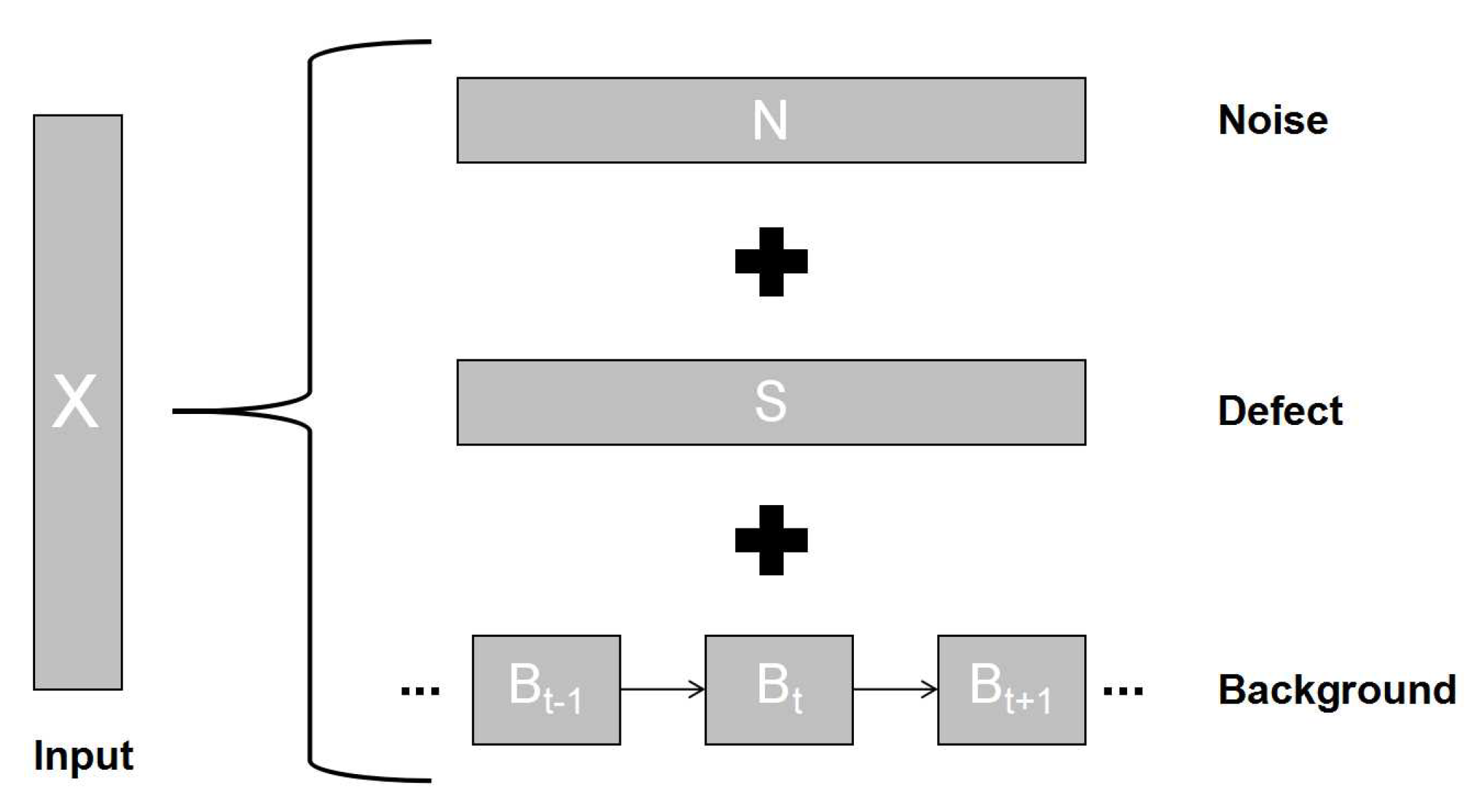
Generally, a track image subject to inspection is relatively consistent and normal, and any defect is equivalent to an abnormal area. From the perspective of matrix analysis, there is a correlation between the gray-scale matrices of the track surface image, and a potential correlation exists between the defect area on the track surface and the background. Recently, low-rank and sparse decomposition methods have shown promising results in foreground detection. The only assumption made regarding the background is that any variation in its appearance can be captured by the low-rank matrix [18]. In this simple form, a matrix composed of the observed data can be decomposed into a low-rank matrix representing the background and a sparse matrix consisting of foreground objects, treated as sparse foreground.

In recent years, sparse coding and low-rank recovery have received considerable attention. Researchers have carried out extensive research on multiple levels of basic theory, algorithms, and applications [19,20,21]. Among them, sparse representation theory has been widely used in the field of computer vision [22,23,24,25] and in many hyperspectral image (HSI) processing fields [26,27]. The theory [28,29,30,31] assumes that an unknown signal can be sparsely represented by a linear combination of several signals from an overcomplete dictionary. The corresponding sparse coding shows a good feature representation ability and can implicitly encode interclass information. Different constraints imposed on the coding, $\mathit{\alpha }$, solve difficult problems associated with different visual tasks. In addition, a series of studies considered the sparse structure of sparse codes or prior knowledge of the spatial distribution of the residual term $\mathbf{e}$ [32,33,34,35]. A typical example is the ProxFlow method. Its objective function is defined as follows:

$$\underset{\mathit{\alpha },\mathbf{e}}{argmin}{∥\mathbf{x}-\mathbf{D}\mathit{\alpha }-\mathbf{e}∥}_2^2+{\lambda }_1{∥\mathit{\alpha }∥}_1+{\lambda }_2{∥\mathbf{e}∥}_{{\ell }_1/{\ell }_{\infty }},$$

(1)

where the input signal, $\mathbf{x}\in {\mathbb{R}}^m$, can be described by a sparse linear representation given the overcomplete dictionary, $\mathbf{D}\in {\mathbb{R}}^{m\times K}$, and a residual term $\mathbf{e}$. Here, the norm of ${\ell }_1/{\ell }_{\infty }$ is the sparse structure. The sparse norm of the structure has been proposed for the first time; it can yield compact foreground detection. However, the ProxFlow method requires a large amount of pure background data for training and to obtain a clean overcomplete dictionary; otherwise a clean background cannot be restored, and complete foreground detection cannot be achieved. In addition, the decomposition method combining low rank and sparseness (low-rank matrix restoration theory) has made great progress in signal processing, pattern recognition, and other fields. The only assumption made is that any change in the background appearance can be captured by the low-rank matrix [18]. In this simple form, the observed data matrix can be decomposed into a sparse matrix [36] and a low-rank matrix, representing the sparse foreground and the background, respectively. This is the well-known robust principal component analysis (RPCA), which has been studied extensively [21,37,38,39,40,41].

The observation matrix $X\in {\mathbb{R}}^{m\times n}$ can be formed by linear superposition of the matrices $\mathbf{L}$ and $\mathbf{S}$, assuming that the singular value of $\mathbf{L}$ is sparse. That is, $\mathbf{L}$ is a low-rank matrix, and the matrix elements in $\mathbf{S}$ are sparse. Then, the low-rank matrix recovery can be expressed as:

$$\begin{array}{c}\underset{\mathbf{L},\mathbf{S}}{\min }{\parallel \mathbf{L}\parallel }_{*}+\lambda {\parallel \mathbf{S}\parallel }_1\\ s.t.\mathbf{x}=\mathbf{L}+\mathbf{S}.\end{array}$$

(2)

If all elements in the matrix can be observed, this problem is also referred to as robust principal component analysis (RPCA). The defined nuclear norm of the matrix (the Nuclear Norm) is the ${\ell }_1$ norm of the singular value vector; i.e., ${\parallel \mathbf{L}\parallel }_{*}={\parallel \overrightarrow{\sigma }\parallel }_1$. The kernel can be easily verified as a convex function. In practical applications, the noise component can also be considered in the superposition equation. The low-rank matrix recovery problem (2) can be described as a semi-definite programming problem, so it is computationally feasible. Candes et al. [18] proved that when the number of samples meets certain conditions, the kernel norm minimization problem can be completely restored with a high probability. If the rank of the matrix is lower, more missing elements can be allowed [18,42]. More theoretical results show that this recovery is also stable in the presence of noise [43]. The matrix representation of input data is more intuitive and convenient. The low-rank representation may be considered a generalization of the sparse vector representation. Low-rank matrix recovery theory has attracted wide attention. It has had an important impact on signal processing, pattern recognition and computer vision. For instance, it has been explored extensively in the application of texture extraction and texture modeling [44,45], face recognition [35], video denoising [46], segmentation [47,48], and to detect moving objects in videos [21], achieving good results.

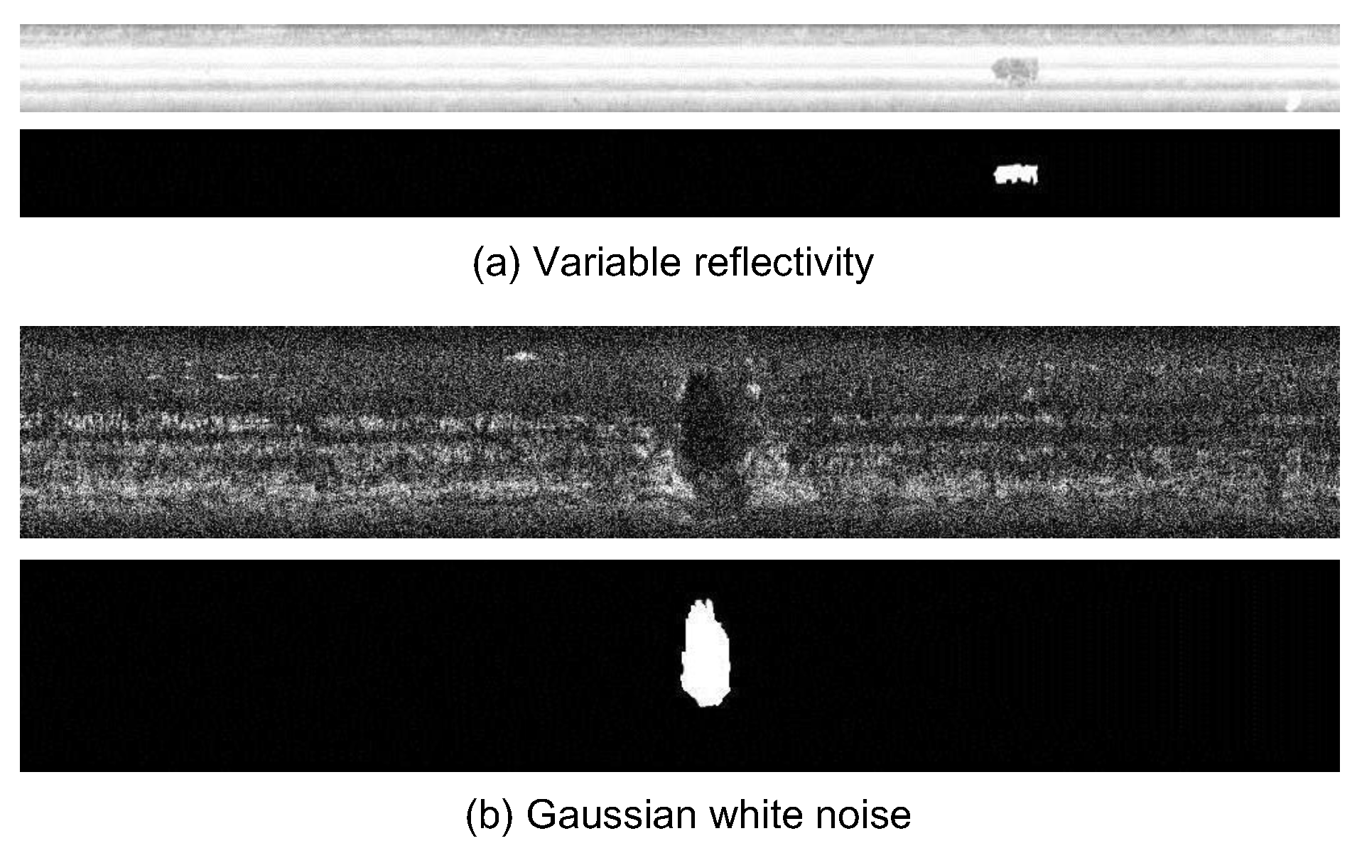
However, according to low-rank matrix recovery theory, when there is high coherence between low-rank and sparse components, the decomposition performance of the observation matrix will be reduced. Therefore, when the background is cluttered or has a similar appearance to that of the salient objects, they are difficult to separate using the previously introduced methods based on low-rank matrix restoration theory. In addition, noise, light, vibration, and other factors will cause the background to appear dynamic, while the low-rank constraint cannot adequately describe this dynamic background change, and some elements of the background are decomposed into sparse components.

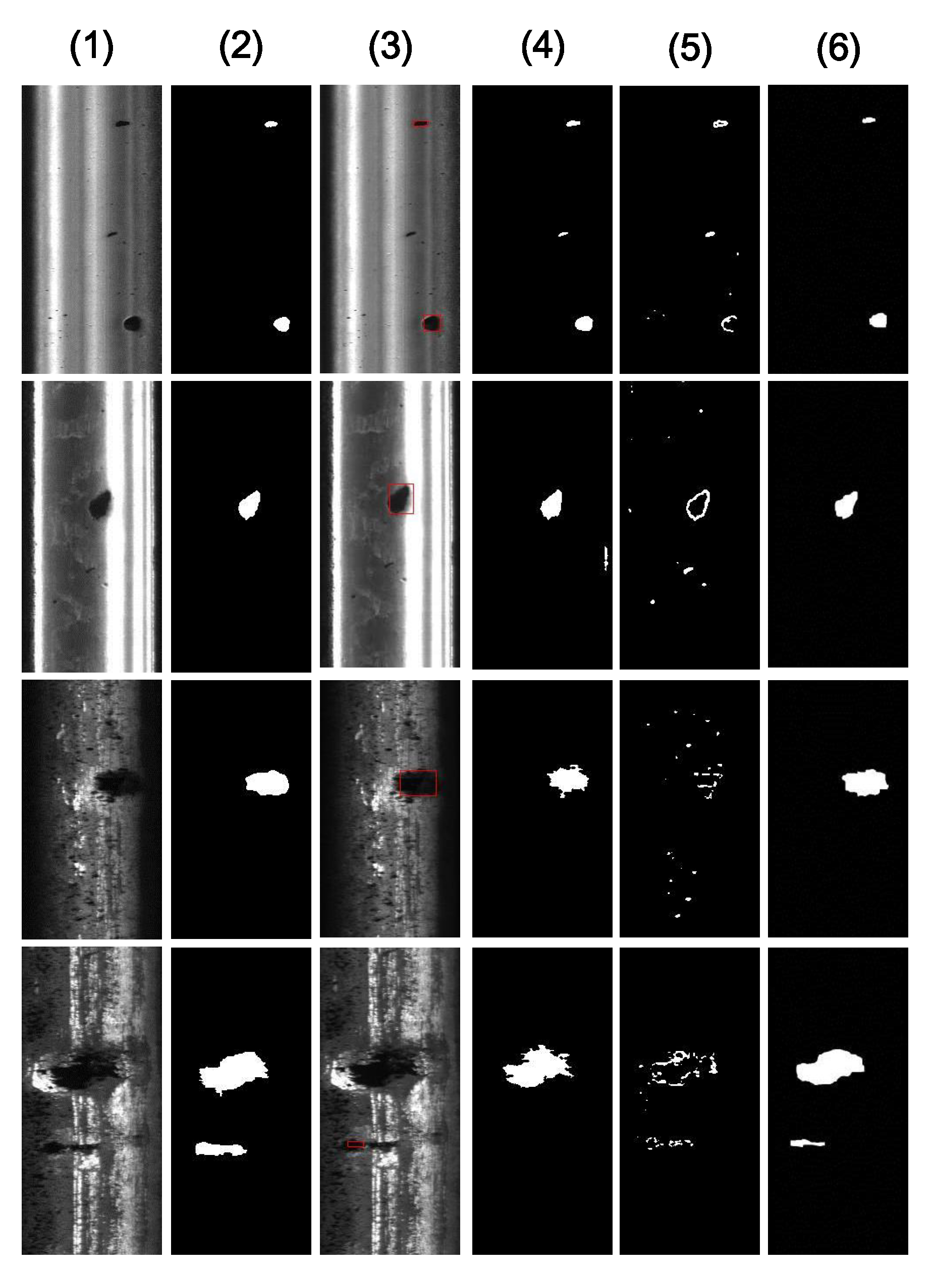
In this paper, we propose a new defect detection model. Specifically, to better describe the dynamic background, we use a differential regular term to describe the background’s dynamic performance. This type of background modeling based on a differential regular term can adequately capture background noise and other factors. To encode the prior spatial structure information of the defect components, we introduce structured sparsity norm constraints and use the hierarchical segmentation tree structure of super pixel blocks to maximize the defect area that is completely absorbed into compact, sparse components. The experimental results show that the proposed model can handle the dynamics of the track surface well and that it can be used for structural inspection of the defect area.

In summary, the main contribution of this paper includes three aspects.

• We propose a general defect detection model and a theoretical framework. Based on low-rank matrix restoration theory, a new defect detection model is proposed. Although the proposed framework is general, this is the first study that introduces a low-rank framework to the field of rail surface inspection and demonstrates its superiority over baseline methods.
• We propose a differential regular term constraint to replace the general low-rank constraint. It can be used to reconstruct the dynamic background and solve the degradation of the decomposition performance when there is high coherence between low-rank and sparse components.
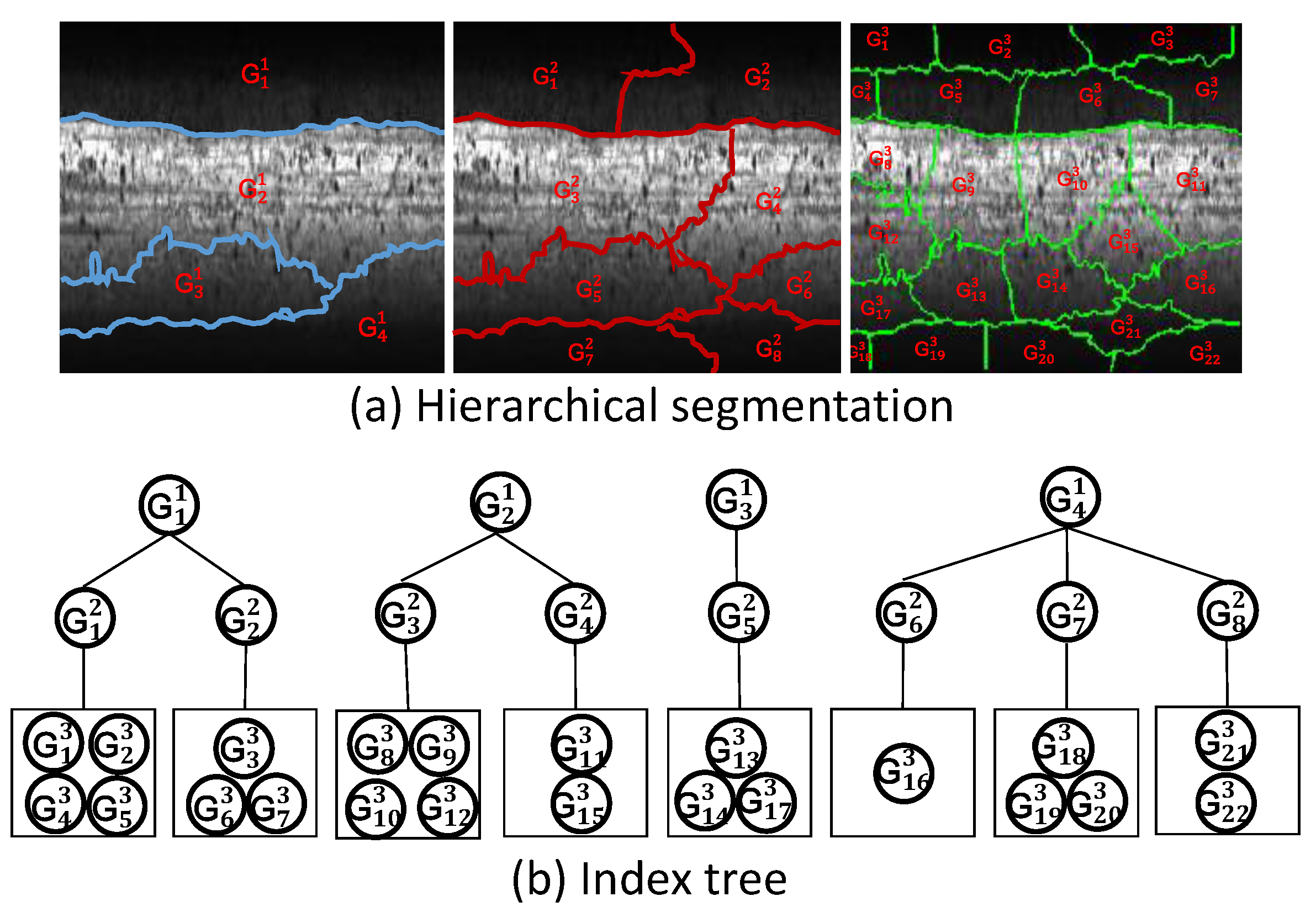
• With regard to the structural sparseness norm constraint, we use the hierarchical tree structure of superpixel segmentation to standardize the sparse components and obtain a more compact and complete defect area. However, the track image has feature limitations, so our study uses structural sparsity constraints applied to the gray levels of superpixel blocks (that is, the gray values of the pixels in the block as well as the block as a whole are drawn as a vector to obtain constraints). This is not equivalent to the use of structural sparsity in the feature space of superpixel blocks, as in several previous studies (that is, a constraint to the matrix imposed by feature vectors between blocks).

The remainder of this paper is organized as follows. Section 2 offers an overview and details of the proposed method. The experimental setup and results are presented in Section 3, followed by our conclusion in Section 4.

2. Decomposition Model for Defects Detection

In this section, we will detail our novel decomposition model for RSDDs inspection, as follows.

2.1. Motivation and Formalization

In the vision-based rail surface defect detection system, the rail surface containing defects can be considered a combination of rail surface background, defect targets, and noise. In computer vision theory, low-rank matrix restoration theory [18,33,49] can handle this situation well. This requires the decomposition of superimposed signals. However, note that defect detection in rail surface images differs from general visual inspection. On the one hand, the background of the rail surface is dynamic; on the other hand, there is a potential correspondence between the defect target and the background in the rail surface image.

Although low-rank matrix restoration theory has achieved good results in computer vision tasks, it still has some problems in the context of the specific task of orbital defect detection in response to the aforementioned two challenges.

• According to low-rank matrix restoration theory, when there is a high correlation between low-rank and sparse components, the decomposition performance of the observation matrix will be reduced. Therefore, when the background is cluttered or has a similar appearance to the detection object, it is difficult for previously developed low-rank matrix recovery models to separate them.
• Low-rank matrix restoration theory cannot well describe the dynamic background in track surface images. For example, impurity elements in the background often do not meet the low-rank constraint and are forcibly decomposed into sparse components. In addition, when the target scale or the span of the defect is large, low-rank matrix recovery theory often decomposes the defect into the background component as a low-rank component.

To solve these problems, we propose a novel matrix factorization model, which regards the defect target and background separation as a problem of dynamic background reconstruction and structural sparse matrix factorization. First, the surface of the track has a different appearance and evolves dynamically over time. Therefore, we adopt a differential strategy rather than low rank for background reconstruction. Second, we introduce a tree-shaped sparse induction norm to constrain the sparse components, so as to consider the spatial structure of image blocks in our matrix decomposition. The entire framework is shown in Figure 1, and the final model is formalized as:

$$\begin{array}{c}\underset{\mathbf{B},\mathbf{S},\mathbf{N}}{\min }\mathsf{\Psi }\left(\mathbf{B}\right)+{\lambda }_1\mathsf{\Omega }\left(\mathbf{S}\right)+{\lambda }_2\mathsf{\Phi }\left(\mathbf{N}\right)\\ s.t.\mathbf{x}=\mathbf{B}+\mathbf{S}+\mathbf{N},\end{array}$$

(3)

where $\mathbf{x}\in {\mathbb{R}}^{m\times n}$ is the input data, $\mathbf{B}$, $\mathbf{S}$, and $\mathbf{N}$ are the corresponding background, defect, and noise levels, respectively; $\mathsf{\Psi }(·)$ is the background’s differential regular term, $\mathsf{\Omega }(·)$ is the structured sparse regular term of the defects, and $\mathsf{\Phi }(·)$ is the sparse regular term of the noise. The additional terms do not only allow our model to capture the basic structure of the dynamic background data, but they also facilitate improved handling of the challenges caused by the coherence between the background and defect data compared with the classic low-rank matrix recovery model; ${\lambda }_1,{\lambda }_2$ are positive hyperparameters.

2.2. Differential Regular Background Term

We regard the observed rail surface data, $\mathbf{x}\in {\mathbb{R}}^{m\times n}$, as a continuous signal. The data matrix, $\mathbf{B}=[\cdots ,{\mathbf{B}}_t,\cdots ]\in {\mathbb{R}}^{m\times n}$, represents the reconstructed background, where ${\mathbf{B}}_t\in {\mathbb{R}}^m$ represents the tth background line along the longitudinal direction. Here we introduce a differential regular term to describe the time-varying nature of the data, which is formalized as:

$$\mathsf{\Psi }\left(\mathbf{B}\right)=\sum _{t=1}^{n-1}{u}_{t,t+1}{\parallel {\mathbf{B}}_{t+1}-{\mathbf{B}}_t\parallel }_2^2,$$

(4)

where $u_{t,t+1}$ represents the correlation weight between the observation data ${\mathbf{x}}_t$ and ${\mathbf{x}}_{t+1}$. If ${\mathbf{x}}_t$ and ${\mathbf{x}}_{t+1}$ are not similar, there may be defects in one of the observed data sets. Therefore, we want to minimize the problem $\mathsf{\Psi }\left(\mathbf{B}\right)$ to construct the real background, forcing the background data ${\mathbf{B}}_t$ to be similar to ${\mathbf{B}}_{t+1}$. Therefore, the correlation weight, $u_{t,t+1}$, is defined as:

$$u_{t,t+1}=exp(\gamma \parallel {\mathbf{x}}_t-{\mathbf{x}}_{t+1}{\parallel }_2),$$

(5)

where $\gamma$ is a hyperparameter and ${\parallel ·\parallel }_2$ is the ${\ell }_2$ norm. In order achieve a more robust result, we normalize the maximum value of the correlation weight, ${\left\{u_{t,t+1}\right\}}_{t=1}^{n-1}$. This definition implies that we consider $u_{t,t+1}$ to explain the coherent changes over time between observational data. Therefore, our model can handle a more challenging scene evolution. Compared with the restricted low-rank constraint, the introduced term adopts a difference operator to relax the background constraint. Therefore, it can adequately describe the dynamic background construction and the large scale or span of defect separation in track surface images.

2.3. The Structured Sparse Regular Term for Defects

Defect areas on rail surfaces are usually spatially continuous and occupy only a small fraction of the scene. Therefore, the use of the structured sparsity norm to model defect areas is highly suitable, because it can reflect a non-zero spatial distribution. Inspired by the latest advances in structural sparsity [33,34,35], we introduce a novel tree-like sparsity-inducing structure specification to simulate spatial continuity and feature similarities between image blocks, thereby generating more accurate and structurally consistent results. First, we define a series of superpixels [50], where each superpixel constitutes a node of a tree. Figure 2a shows that there is no overlap between node indices. Second, we use the index tree, T, to encode the spatial relationship between the super-pixels. The index tree structure is shown in Figure 2b. The index tree is a hierarchical structure, so that each node contains a set of indices (for example, corresponding to the superpixels in our task), and the set is the union of the indices of its child nodes. More specifically, the series of superpixels thus obtained is clustered at different levels to obtain the hierarchical segmentation result, as shown in Figure 2a. For an index tree T with a depth d, ${\mathcal{G}}^i$ represents the set of all nodes at the ith level. For example, for the root node, we have ${\mathcal{G}}^1$ containing four node sets, $G_1^1,G_2^1,G_3^1$, and $G_4^1$; ${\mathcal{G}}^3$ then represents the series of superpixel collections we obtained originally, as shown in Figure 2. We encode structurally meaningful tree constraints as sparse norms and decompose them with the normalized matrix. This way, we achieve sparse regularization of the general tree structure. This type of hierarchical tree structure constraint induces superpixels in the same group that share similar representations. This also expresses the subordination or coordinate relationship between groups, which is specifically formalized as ${\displaystyle \sum _{i=1}^d}{\displaystyle \sum _{g\in {\mathcal{G}}_i}}{\parallel {\mathbf{S}}_g^i\parallel }_p$, where ${\mathbf{S}}_g^i$ represents the set of all pixels contained in a node in the ith layer node set. Here we pull this set into a vector representation to facilitate norm operations, that is, ${\mathbf{S}}_g^i$ is a vector.

We know that the ${\ell }_1$ norm deals with the corresponding elements independently, so spatial structure information is ignored. We therefore introduce the ${\ell }_{\infty }$ norm. The ${\ell }_{\infty }$ norm is the maximum value of the pixels in the group. It encourages other pixels to adopt arbitrary values. We can expect similar error regions to have similarly large values; minimizing the objective function emphasizes the structure of distributed sparse outliers. To illustrate this advantage, we assume that there are two different distributions of sparse foreground in our $8\times 8$ image (see Figure 3), where white pixels correspond to outliers with high values, and black pixels correspond to the background. For convenience of presentation, we have divided the image into three simple superpixels, as shown in Figure 3. Since the ${\ell }_1$ norm combines the absolute values of all pixels, this sparse norm constraint will have similar values in the two sparse distribution cases. However, for the ${\ell }_{\infty }$ norm, only the largest value in each pre-designed group is included, which leads to significantly different values between both sparse distributions. This example shows that the ${\ell }_1$ norm processes each pixel independently, while the structured sparseness based on the ${\ell }_{\infty }$ norm can consider possible relationships among subsets of entries. On this basis, we further summarize the structured sparse regular term proposed to describe the defect:

$$\mathsf{\Omega }\left(\mathbf{S}\right)=\sum _{i=1}^d\sum _{g\in {\mathcal{G}}_i}{\parallel {\mathbf{S}}_g^i\parallel }_{\infty }.$$

(6)

This constraint is essentially a sparseness specification of hierarchical groups based on a tree structure, where the ${\ell }_{\infty }$ norm is used to force internal elements to share a consistent saliency value. This regularization considers the hierarchy of the spatial structure in the image and eventually separates the defect area from the background to the extent possible. These attributes enable our model to detect defective objects on the rail surface, even if there is a potential correlation between the defect and the background.

2.4. Optimization

Based on the aforementioned definition, the specific form of our model is:

$$\begin{array}{c}\underset{\mathbf{B},\mathbf{S},\mathbf{N}}{\min }{\displaystyle \sum _{t=1}^{n-1}}{u}_{t,t+1}{\parallel {\mathbf{B}}_{t+1}-{\mathbf{B}}_t\parallel }_2^2+\\ {\lambda }_1{\displaystyle \sum _{i=1}^d}{\displaystyle \sum _{g\in {\mathcal{G}}_i}}\parallel {\mathbf{S}}_g^i{\parallel }_{\infty }+{\lambda }_2{\parallel \mathbf{N}\parallel }_{1,1}\\ s.t.\mathbf{x}=\mathbf{B}+\mathbf{S}+\mathbf{N}.\end{array}$$

(7)

Considering a practical balance between efficiency and accuracy, we use the Alternating Direction Method (ADM) [51] to optimize the solution model (7). The minimized problem (7) then becomes:

$$\begin{array}{c}\mathcal{L}(\mathbf{B},\mathbf{S},\mathbf{N},\mathbf{Y},\mu )={\displaystyle \sum _{t=1}^{n-1}}{u}_{t,t+1}{\parallel {\mathbf{B}}_{t+1}-{\mathbf{B}}_t\parallel }_2^2+\\ {\lambda }_1{\displaystyle \sum _{i=1}^d}{\displaystyle \sum _{g\in {\mathcal{G}}_i}}\parallel {\mathbf{S}}_g^i{\parallel }_{\infty }+{\lambda }_2{\parallel \mathbf{N}\parallel }_{1,1}+\\ Tr\left({\mathbf{Y}}^T(\mathbf{x}-\mathbf{B}-\mathbf{S}-\mathbf{N})\right)+\frac{\mu }{2}{\parallel \mathbf{x}-\mathbf{B}-\mathbf{S}-\mathbf{N}\parallel }_F^2.\end{array}$$

(8)

Here, $\mathbf{Y}$ is the Lagrangian multiplier and $\mu >0$ is the linear constraint penalty. We apply a continuously iterative alternate optimization strategy to optimize $\mathbf{B},\mathbf{S},\mathbf{N}$. The full optimization process is shown in Algorithm 1. Below, we will discuss the detailed steps involved in each iteration.

Update $\mathbf{B}$: When $\mathbf{S}$ and $\mathbf{N}$ are fixed, the optimization problem of updating ${\mathbf{B}}^{k+1}$ in the $(k+1)$th iteration is as follows:

$$\begin{array}{cc}\hfill {\mathbf{B}}^{k+1}& =\underset{\mathbf{B}}{argmin} \mathcal{L}(\mathbf{B},{\mathbf{S}}^k,{\mathbf{N}}^k,{\mathbf{Y}}^k,{\mu }^k)\hfill \\ \hfill & =\underset{\mathbf{B}}{argmin}\sum _{t=1}^{n-1}{u}_{t,t+1}{\parallel {\mathbf{B}}_{t+1}-{\mathbf{B}}_t\parallel }_2^2+\hfill \\ \hfill & Tr({({\mathbf{Y}}^k)}^T(\mathbf{x}-\mathbf{B}-{\mathbf{S}}^k-{\mathbf{N}}^k))+\hfill \\ \hfill & \frac{{\mu }^k}{2}{\parallel \mathbf{x}-\mathbf{B}-{\mathbf{S}}^k-{\mathbf{N}}^k\parallel }_F^2.\hfill \end{array}$$

(9)

To facilitate finding the solution of $\mathbf{B}$, we introduce a differential auxiliary variable,

$$\mathbf{F}=\left(\begin{array}{cccc}-1& 0& \cdots & 0\\ 1& -1& \cdots & 0\\ ⋮& ⋮& \ddots & ⋮\\ 0& 0& \cdots & 1\end{array}\right)\in {\mathbb{R}}^{n\times (n-1)}.$$

(10)

The above problem can then be simplified as:

$$\begin{array}{cc}\hfill {\mathbf{B}}^{k+1}=& \underset{\mathbf{B}}{argmin} \frac{{\mu }^k}{2}{\parallel {\mathbf{T}}_B-\mathbf{B}\parallel }_F^2+\hfill \\ & Tr(\left(\mathbf{B}\mathbf{F}\right)\mathbf{U}{\left(\mathbf{B}\mathbf{F}\right)}^T),\hfill \end{array}$$

(11)

where $\mathbf{U}=diag\left([u_{1,2},u_{2,3},\cdots ,u_{n-1,n}]\right)$ and ${\mathbf{T}}_B=\mathbf{x}-{\mathbf{S}}^k-{\mathbf{N}}^k+{\left({\mu }^k\right)}^{-1}{\mathbf{Y}}^k$. Furthermore, since $\mathbf{U}$ is a positive definite diagonal matrix with respect to its weights (all values are greater than 0), $\mathbf{U}={\mathbf{U}}^{\frac{1}{2}}{\left({\mathbf{U}}^{\frac{1}{2}}\right)}^T$ is established and the above formula is further simplified to:

$${\mathbf{B}}^{k+1}=\underset{\mathbf{B}}{argmin} \frac{{\mu }^k}{2}\parallel {\mathbf{T}}_B{-\mathbf{B}\parallel }_F^2+{\parallel \mathbf{B}\mathbf{F}{\mathbf{U}}^{\frac{1}{2}}\parallel }_F^2.$$

(12)

It can be easily concluded that the above problem represents the convex function; the solution can be obtained by directly deriving $\mathbf{B}$. Then, for the optimal solution of ${\mathbf{B}}^{k+1}$, the following closed-form solutions are present:

$${\mathbf{B}}^{k+1}={\mu }^k{({\mu }^k+2\mathbf{F}\mathbf{U}{\mathbf{F}}^T)}^{+}{\mathbf{T}}_B,$$

(13)

where ${(·)}^{+}$ represents the pseudo-inverse of the matrix.

Algorithm 1 Our model optimization steps

Input:  Given input data $X\in {\mathbb{R}}^{m\times n}$, correlation weight $u_{t,t+1}$, parameters ${\lambda }_1,{\lambda }_2$, and Index tree T; Output:  ${\mathbf{B}}^{*},{\mathbf{S}}^{*},{\mathbf{N}}^{*}$; 1: Initialization: ${\mathbf{B}}^0=\mathbf{0},{\mathbf{S}}^0=\mathbf{0},{\mathbf{N}}^0=\mathbf{0},\mathbf{Y}=\mathbf{0},\rho =1.1,{\mu }^0=0.1,{\mu }_{\max }={10}^{10}$ and $k=0$; 2: while not convergent do 3:     Update $\mathbf{B}$: ${\mathbf{B}}^{k+1}=\underset{\mathbf{B}}{argmin} \mathcal{L}(\mathbf{B},{\mathbf{S}}^k,{\mathbf{N}}^k,{\mathbf{Y}}^k,{\mu }^k)$; 4:     Update $\mathbf{S}$: ${\mathbf{S}}^{k+1}=\underset{\mathbf{S}}{argmin} \mathcal{L}({\mathbf{B}}^{k+1},\mathbf{S},{\mathbf{N}}^k,{\mathbf{Y}}^k,{\mu }^k)$; 5:     update $\mathbf{N}$: ${\mathbf{N}}^{k+1}=\underset{\mathbf{N}}{argmin} \mathcal{L}({\mathbf{B}}^{k+1},{\mathbf{S}}^{k+1},\mathbf{N},{\mathbf{Y}}^k,{\mu }^k)$; 6:     ${\mathbf{Y}}^{k+1}=\mathbf{Y}+{\mu }^k(X-{\mathbf{B}}^{k+1}-{\mathbf{S}}^{k+1}-{\mathbf{N}}^{k+1})$; 7:     ${\mu }^{k+1}=min(\rho {\mu }^k,{\mu }_{\max })$;$k\leftarrow k+1$ 8: end while

Update $\mathbf{S}$: If $\mathbf{B}$ and $\mathbf{N}$ are fixed, the optimization problem of updating ${\mathbf{S}}^{k+1}$ in the $(k+1)$th iteration is as follows:

$$\begin{array}{cc}\hfill {\mathbf{S}}^{k+1}& =\underset{\mathbf{S}}{argmin} \mathcal{L}({\mathbf{B}}^{k+1},\mathbf{S},{\mathbf{N}}^k,{\mathbf{Y}}^k,{\mu }^k)\hfill \\ \hfill & =\underset{\mathbf{S}}{argmin} {\lambda }_1{\displaystyle \sum _{i=1}^d}{\displaystyle \sum _{g\in {\mathcal{G}}_i}}{\parallel {\mathbf{S}}_g^i\parallel }_{\infty }+\hfill \\ \hfill & Tr({({\mathbf{Y}}^k)}^T(\mathbf{x}-{\mathbf{B}}^{k+1}-\mathbf{S}-{\mathbf{N}}^k))+\hfill \\ \hfill & \frac{{\mu }^k}{2}{\parallel \mathbf{x}-{\mathbf{B}}^{k+1}-\mathbf{S}-{\mathbf{N}}^k\parallel }_F^2\hfill \\ \hfill & =\underset{\mathbf{S}}{argmin} {\lambda }_1{\displaystyle \sum _{i=1}^d}{\displaystyle \sum _{g\in {\mathcal{G}}_i}}\parallel {\mathbf{S}}_g^i{\parallel }_{\infty }+\frac{{\mu }^k}{2}{\parallel {\mathbf{T}}_S-\mathbf{S}\parallel }_F^2,\hfill \end{array}$$

(14)

where ${\mathbf{T}}_S=\mathbf{x}-{\mathbf{B}}^{k+1}-{\mathbf{N}}^k+{\left({\mu }^k\right)}^{-1}{\mathbf{Y}}^k$. The above problems can be solved using the hierarchical proximal operator [52]. In simple terms, the operator calculates a specific residual sequence for optimization by projecting the matrix onto the unit ball of the dual ${\ell }_p$ norm. The detailed steps for the norm of ${\ell }_{\infty }$ in question (14) are given in Algorithm 2.

Algorithm 2 Update of the algorithm steps of $\mathbf{S}$

Input:  All nodes in the index tree set ${\mathcal{G}}^i$ ($i=1,\cdots ,d$), matrix ${\mathbf{T}}_S$, parameters ${\lambda }_1,{\mu }^k$, and set $\lambda =\frac{{\lambda }_1}{{\mu }^k}$; Output:  ${\mathbf{S}}^{k+1}$; 1: Initialization $\mathbf{S}={\mathbf{T}}_S$; 2: for$i=d$ to 1 do 3:      for $\forall g\in {\mathcal{G}}_i$ do $${\left({\mathbf{S}}_g^i\right)}^{k+1}=\left\{\begin{array}{cc}\frac{\parallel {\mathbf{S}}_g^i{\parallel }_1-\lambda }{\parallel {\mathbf{S}}_g^i{\parallel }_1}{\mathbf{S}}_g^i,\hfill & \mathrm{if}\parallel {\mathbf{S}}_g^i{\parallel }_1>\lambda \hfill \\ 0,\hfill & \mathrm{otherwise}\hfill \end{array}\right.$$ 4:     end for 5: end for

Update $\mathbf{N}$: If $\mathbf{B}$ and $\mathbf{S}$ are fixed, the optimization problem of updating ${\mathbf{N}}^{k+1}$ in the $(k+1)$th iteration is as follows:

$$\begin{array}{cc}\hfill {\mathbf{N}}^{k+1}& =\underset{\mathbf{N}}{argmin} \mathcal{L}({\mathbf{B}}^{k+1},{\mathbf{S}}^{k+1},\mathbf{N},{\mathbf{Y}}^k,{\mu }^k)\hfill \\ \hfill & =\underset{\mathbf{N}}{argmin} {\lambda }_2{\parallel \mathbf{N}\parallel }_{1,1}+\hfill \\ \hfill & Tr({\left({\mathbf{Y}}^k\right)}^T(\mathbf{x}-{\mathbf{B}}^{k+1}-{\mathbf{S}}^{k+1}-\mathbf{N}))+\hfill \\ \hfill & \frac{{\mu }^k}{2}{\parallel \mathbf{x}-{\mathbf{B}}^{k+1}-{\mathbf{S}}^{k+1}-\mathbf{N}\parallel }_F^2\hfill \\ \hfill & =\underset{\mathbf{N}}{argmin} {\lambda }_2{\parallel \mathbf{N}\parallel }_{1,1}+\frac{{\mu }^k}{2}{\parallel {\mathbf{T}}_N-\mathbf{N}\parallel }_F^2,\hfill \end{array}$$

(15)

where ${\mathbf{T}}_N=\mathbf{x}-{\mathbf{B}}^{k+1}-{\mathbf{S}}^{k+1}+{\left({\mu }^k\right)}^{-1}{\mathbf{Y}}^k$. This problem can be solved using a soft-thresholding operator. Specifically, ${\mathbf{N}}^{k+1}={\mathcal{S}}_{{\lambda }_2/{\mu }^k}\left({\mathbf{T}}_N\right)$, where ${\mathcal{S}}_{\lambda }\left(v\right)=sign\left(v\right)max(0,|v-\lambda \left|\right)$.

The convergence condition of the algorithm is that the decomposition’s relative error of the input matrix $\mathbf{x}$ is less than the tolerance $ϵ$. The decomposed background matrix, $\mathbf{B}$, the defect matrix, $\mathbf{S}$, and the noise matrix, $\mathbf{N}$, correspond to relative changes. They are less than the tolerance $ϵ$, formalized as $\parallel \mathbf{x}-{\mathbf{B}}^k-{\mathbf{S}}^k-{\mathbf{B}}^k{\parallel }_F/{\parallel \mathbf{x}\parallel }_F<ϵ\&\&max(\parallel {\mathbf{B}}^k-{\mathbf{B}}^{k-1}{\parallel }_F/{\parallel \mathbf{x}\parallel }_F,\parallel {\mathbf{S}}^k-{\mathbf{S}}^{k-1}{\parallel }_F/{|\mathbf{x}\parallel }_F,\parallel {\mathbf{N}}^k-{\mathbf{N}}^{k-1}{\parallel }_F/{\parallel \mathbf{x}\parallel }_F)<ϵ$, where $ϵ={10}^{-7}$ is set in the experiment. We found experimentally that the algorithm is not sensitive to a wide range of values of $ϵ$.

3. Experimental Results and Analysis

In this section, we detail our experimental setup and report the performance of the proposed method.

3.1. Experimental Setup

To evaluate the performance of our method for RSDDs inspection, we implemented the proposed method in Matlab R2015 and collected two data sets. The first was a Type-I RSDDs data set captured from express rails, which contained 67 images. The second was a Type-II RSDDs data set captured from common/heavy-haul rails, which contained 128 images. Note that each image in both data sets contained at least one defect as well as a dynamic background with much noise (the two data sets are available at: http://icn.bjtu.edu.cn/Visint/resources/RSDDs.aspx (accessed on 15 August 2020)). This paper focuses on the detection of track surface defects. Therefore, to reduce interference by irrelevant information and improve the detection performance, in each track image acquired by the system we used an algorithm based on projection contours [12] to remove other components on either side of the track (e.g., fasteners, sleepers, bolts and ballast). In our model, we set ${\lambda }_1=5$ and ${\lambda }_2=0.01$ to achieve a balance between background reconstruction and defect extraction.

To quantitatively evaluate the proposed method, we adopted criteria related to Precision, Recall, and F1-measure, which are widely used in the pattern recognition and information retrieval communities [53]. In addition, two types of evaluation indices from different perspectives (i.e., pixel- and defect-level) were adopted to completely evaluate our method for RSDDs inspection.

Pixel-level index. $Pre$, $Rec$, and F1-measure (F) are defined as:

$$\begin{array}{cc}& Pre=TP/(TP+FP)\\ & Rec=TP/(TP+FN)\end{array}$$

$$\begin{array}{cc}& F=2\ast Pre\ast Recall/(Pre+Rec),\end{array}$$

(16)

where $TP$ denotes the number of correctly detected points, $FP$ is the number of incorrectly defective points, and $FN$ is the number of undetected defective points. There is an inverse relationship between precision and recall. That is, it is possible to increase one at the cost of reducing the other. Hence, F1-measure was introduced. The higher F1-measure is, the more the detection result is consistent with human judgment. Note that $Pre$, $Rec$, and F reported in the following experiments are average values for the whole data set.

Defect-level index. $Pr{e}^{\prime }$, $Re{c}^{\prime }$, and F1-measure ($F^{\prime }$) are defined as:

$$\begin{array}{cc}& Pr{e}^{\prime }=TP/P\\ & Re{c}^{\prime }=T{P}^{\prime }/N\end{array}$$

$$\begin{array}{cc}& F^{\prime }=2\ast Pr{e}^{\prime }\ast Re{c}^{\prime }/(Pr{e}^{\prime }+Re{c}^{\prime }),\end{array}$$

(17)

where $TP$ denotes the number of correctly detected defects, $T{P}^{\prime }$ is the number of correctly detected defects mapping to ground truth, P refers to the total number of detected defects, and N refers to the total number of labeled defects in the ground truth. Note that the numbers counted for $Pr{e}^{\prime }$ and $Re{c}^{\prime }$ pertain to the whole data set.

3.2. Evaluation

The proposed method is consistent with other classic decomposition models. It is an algorithm that continuously and iteratively updates the background, foreground, and noise levels. Figure 4 shows the iteration of the proposed method. Our method can generally achieve good decomposition results after five iterations. Note that the background, foreground, and noise levels are all initialized to the $\mathbf{0}$ matrix. Based on our experiments, the background and defects all begin to appear after one iteration. The background can be adequately reconstructed and the compactness and integrity of the defects are also adequately reflected after five iterations. Iterations will continue until the convergence conditions set by the algorithm are met and a stable component decomposition is achieved.

The detection of track surface defects faces many challenges, such as serious uneven light reflection and edge effects in curved rails, the variability of high-speed railway operating environments, image degradation and dynamic backgrounds caused by the influence of various climatic conditions, and discrete defects having their own multi-scales and diversified characteristics, among others. To verify the robustness of the method, images obtained under extreme lighting conditions, uneven reflections, and track surfaces with dynamic background images were selected. The result is shown in Figure 5. Experiments show that our method still performs well under these extreme conditions and can still correctly extract defect regions and reconstruct the background.

Our method can achieve a robust performance because, on the one hand, the elements to achieve robust detection come from the linear dynamic regular term of the background we proposed, which uses a linear dynamic characterization matrix to describe a linear relationship evolving with time in the track sequence data to realize the reconstruction of the dynamic background. On the other hand, it uses a tree-like hierarchical structure to standardize the structural information of the defect area and obtains compact defects while suppressing noise and other anomalies.

3.3. Comparison and Analysis

3.3.1. The Type-I RSDDs Data Set

Here, further segmentation from the decomposed foreground map using a fixed threshold yields precise defect shapes, which is beneficial for quantitative evaluation and comparison with other well-established methods. Following other fault inspection approaches such as can-end [54], LCD panel [55], and large-aperture optical elements [56], a fixed threshold was adopted. Note that the parameter T influences the performance of defect detection; its impact is shown in Figure 6. As expected, the F1-measure increases when T increases, and our method achieves its best performance for $T=0.17$ because this value results in a good balance between Precision and Recall.

We next compared the inspection performance of the proposed method with other well-established methods in literature, including LN+DLBP, MLC+PEME, and the method of [14]. The parameters of these comparative methods are chosen similarly to our method. Specifically, the upper bound of the defect proportion, $dp$, is set to 0.3 in LN+DLBP, the contribution controlling parameter, $\alpha$, is set to 10 in MLC+PEME, and the gradient threshold, k, and the control parameter, C, of [14] are set to $k=10$ and $C=5$, respectively. The other parameters in these methods are the default values. Figure 7 visualizes some defects selected in the Type-I RSDDs data set and the corresponding inspection results from the different methods. Note that we visualized only the defect part of the rail surface image, for convenience. These comparison methods have good inspection results when the defects and background have characteristics of versatility and consistency, respectively. However, when the internal appearance of the defect is diverse, MLC+PEME results in a larger false negative because the threshold determined by maximizing the entropy is not optimal in MLC+PEME. In addition, the method of [14] is very sensitive to gradients, which will cause large false positives when the background is complex. From the comparison results it transpires that our method yields good inspection results, with neither false positives nor false negatives.

Two types of evaluation indices were used to evaluate performance, and the comparison results are shown in

Table 1. Comparison between our method and the other methods for the Type-I RSDDs data set.

Approach	$\mathit{Pre}$	$\mathit{Rec}$	F	${\mathit{Pre}}^{\prime }$	${\mathit{Rec}}^{\prime }$	${\mathit{F}}^{\prime }$
LN+DLBP	–	–	–	76.26	70.80	73.43
MLC+PEME	78.14	78.89	75.70	47.87	85.40	61.35
Method of [14]	–	–	–	41.19	72.94	52.65
Our method	86.91	82.01	82.86	90.54	81.12	85.57

. Note that LN+DLBP adopts a projection algorithm to locate defects using bounding boxes, and the method of [14] detects contours to locate possible defects. Therefore, pixel-level indinces are not suitable for these two methods. MLC+PEME and the method of [14] have low $Pr{e}^{\prime }$ values when they meet backgrounds that share significantly varying gray-level distributions. Table 1 shows that the F1-measures (F and $F^{\prime }$) of the proposed method are greatly improved with respect to the baseline methods. For a rail image with a dynamic background, the performance of the proposed model depends mostly on the differential regularization term of the background, thereby avoiding absorbing the elements of the background into the sparse components.

3.3.2. The Type-II RSDDs Data Set

First, we again evaluate the dependence on the threshold, T. The appropriate parameter was selected using the same approach as for the Type-I RSDDs data set. Note that T was also chosen by maximizing its corresponding F1-measure (F and $F^{\prime }$). Figure 8 shows the F1-measure curves for T from 0 to 1. As T increases, the two curves increase and then decrease, since precision and recall are inversely correlated. In our experiments, we therefore set T to 0.12, which results in a good balance between Precision and Recall.

We also compared the inspection performance of the proposed method with LN+DLBP, MLC+PEME, and the method of [14]. Note that the parameters of these comparative methods were determined in the same way as for the BODI method, and the parameter settings were as follows. The upper bound to defect proportion, $dp$, was set to 0.3 in LN+DLBP, the contribution controlling parameter, $\alpha$, was set to 3 in MLC+PEME, and the gradient threshold, k, and control parameter, C, of [14] were set to $k=4$ and $C=5$, respectively. The other parameters in these methods were kept at the default values. Figure 9 shows a comparison for these methods. As expected, all methods achieved competitive performance levels for defects that shared universal characteristics. Compared with the Type-I data set, the Type-II RSDDs data set has a more consistent background although more complex defects involving various appearances in its internal and shares different characteristics with other defects. When faced with a complex and dynamic background, our method can achieve promising performance, indicating that the background-based linear dynamic regularization term has more advantages than traditional defect-focusing methods.

We further evaluated our method by comparing two types of evaluation indices, shown in

Table 2. Comparison between our method and the other methods for the Type-II RSDDs data set.

Approach	$\mathit{Pre}$	$\mathit{Rec}$	F	${\mathit{Pre}}^{\prime }$	${\mathit{Rec}}^{\prime }$	${\mathit{F}}^{\prime }$
LN+DLBP	–	–	–	88.89	71.82	79.45
MLC+PEME	73.88	83.05	76.05	58.68	91.71	71.56
Method of [14]	–	–	–	49.73	46.41	48.01
Our method	83.21	80.29	80.72	86.31	80.69	83.41

. LN+DLBP and the method of [14] were also only evaluated using a defect-level index. The method of [14] performed worse than the other methods because of the varying appearances of the defects. Our method achieved the best performance of all baseline methods in terms of F and $F^{\prime }$. This result indicates that matrix decomposition is an attractive strategy, and it is more suitable for the specified inspection task.

3.4. Practical Test

To further evaluate the performance of the proposed method, we conducted an evaluation using an ordinary rail railway line covering 18 km, storing 18,125 individual surface images. These images were captured by an automatic rail image acquisition system, which has an embedded control block automatically controlling LED light sources to adjust their brightness and ensure image quality. The employed CCD camera was an industrial Dalsa Spyder high-speed line-scan camera (maximum line rate of 65,000 lines/s) equipped with an automatic variable-rate filter attenuation system. A PC-Camlink frame grabber connecting the camera and an on-board computer is responsible for the high-speed coding and transmission of images captured by the camera. Several groups of LEDs are installed under a train carriage to eliminate most external stray light. In addition, the camera is triggered by a wheel encoder to ensure that each pixel of a captured image has the same physical size. The acquisition system is installed under a train carriage. It automatically generates one image per meter traveled by the testing train.

We also compared the inspection performance of the proposed method with the other three mature methods. Note that since the images were collected from common/heavy-haul rails, the threshold, T, in our method is still set to 0.12. In addition, note that defective ground-truth markings in railway lines can impose a serious workload. Therefore, we used the number of correct detections, the number of false detections, the number of missed detections, and the correct detection rate to achieve a quantitative evaluation.

Table 3. Statistics of the inspection results for the actual rail line.

Approach	Defect Number	Correct Inspection	False Inspection	Missing Inspection	Inspection Rate
LN+DLBP		15	248	6	71.43%
MLC+PEME		19	27,851	2	90.48%
Method of [14]	21	16	21,098	5	76.19%
Our method		21	373	0	100%

summarizes the quantitative evaluation results of these four comparison methods. From the experimental results, it is found that although LN+DLBP has a low number of false detections, it misses some real defects, and these defects may lead to potential risks in the daily operation of the railway. As expected, MLC+PEME and the method of [14] performed poorly in terms of false detections. Our proposed method can successfully detect all defects and reach the current best detection performance in terms of the correct detection rate. This proves its powerful function in track surface defect detection and further verifies the robustness of the threshold parameter, T, selection.

3.5. Discussion

To further demonstrate its effectiveness, we compare the detection performance of the proposed model with other mature and classic models in the literature, including the principal component pursuit (PCP) model [18] with ${\ell }_1$ norm constraints and the DECOLOR with MRF smoothing constraints (DEC) model [21]. In the original PCP model, $\lambda$ ($\lambda =b/\sqrt{max(m,n)},b=1$) is extremely sensitive to foreground detection. In the detection task, we adopt $\lambda ,b=0.1$. One can use a smaller value to facilitate a more complete detection of the foreground [32]. We adopt $\lambda =1$ in the DEC model to achieve good detection of track defects. Figure 10 shows the comparative detection results. When the track surface is homogeneous and has high-contrast defects and a relatively uniform background, these models can achieve good detection results. Using PCP with ${\ell }_1$ norm constraints, the detection of defect components is scattered, resulting in fragmented detection, whereas the defects separated by our model based on the structural sparsity constraint and the DEC model based on the MRF smoothing constraint are relatively compact and complete. Judging from the decomposition results of rail images with a dynamic background, our model has obvious advantages. On the one hand, the low-rank matrix recovery theory [18] has difficulties separating low-rank and sparse components with high correlation, resulting in more impurities in the defective components. On the other hand, background reconstruction based on low-rank constraints can easily absorb defects on larger scales or spans into the background component, resulting in failure during defect separation. Our method does not only reconstruct a dynamic background, but also obtains a compact and complete defect area without impurity interference. The comparison results shown in

Table 4. Comparative results of PCP, DEC, and our method.

	Approach	$\mathit{Pre}$	$\mathit{Rec}$	F	${\mathit{Pre}}^{\prime }$	${\mathit{Rec}}^{\prime }$	${\mathit{F}}^{\prime }$
Type-I RSDD data set	PCP	74.41	71.27	72.30	75.11	71.43	73.22
	DEC	79.56	75.12	76.08	81.39	77.76	79.53
	Our method	86.91	82.01	82.86	90.54	81.12	85.57
Type-II RSDD data set	PCP	73.14	70.67	71.45	74.32	71.08	72.66
	DEC	76.97	73.68	74.13	78.32	74.95	76.60
	Our method	83.21	80.29	80.72	86.31	80.69	83.41

show that the model performs well on our Type-I and Type-II RSDD data sets.

4. Conclusions

In this paper, we have presented a novel decomposition model for rail defect inspection, assuming that the defected rail image can be represented as the superposition of background, defect, and noise components. Specifically, a differential regular term for the background instead of the commonly used low rank is applied to construct a dynamic background and address the decomposition problem of high coherence between sparse and background components. In the structure sparsity regularization term, the tree structure of superpixels is adopted to constrain the sparse components and obtain more compact and complete defect regions. The experimental results show that the proposed model can achieve better decomposition performance, compared with other typical decomposition models. In terms of pixel- and defect-level indices, the proposed method outperforms existing methods based on extensive RSDDs inspection. In the case of large-facility rail inspection, our method achieves a 100% inspection rate and a low false inspection rate, delivering a promising RSDDs inspection performance. To this end, we explored the most essential mathematical properties of defect structure data and propose a general framework and practical algorithms for other fault inspections in industrial products with a relatively consistent background, such as fabric or paper.

Although the proposed framework can be extended easily to other visual inspection tasks and has a better decomposition performance than other classic matrix factorization models, a number of false positives in the detection of track surface defects remain. In the future, we will focus on the specific task of rail surface detection, dedicated to exploring the inherent space–time characteristics of the orbit and fully collecting and utilizing this information.

References

1. Edwards, R.S.; Dixon, S.; Jian, X. Characterisation of defects in the railhead using ultrasonic surface waves. NDT E Int. 2006, 39, 468–475. [Google Scholar] [CrossRef]
2. Tsai, D.M.; Wu, S.C.; Chiu, W.Y. Defect detection in solar modules using ICA basis images. IEEE Trans. Ind. Inform. 2013, 9, 122–131. [Google Scholar] [CrossRef]
3. Mazzeo, P.L.; Nitti, M.; Stella, E.; Distante, A. Visual recognition of fastening bolts for railroad maintenance. Pattern Recognit. Lett. 2004, 25, 669–677. [Google Scholar] [CrossRef]
4. Aytekin, Ç.; Rezaeitabar, Y.; Dogru, S.; Ulusoy, İ. Railway Fastener Inspection by Real-Time Machine Vision. IEEE Trans. Syst. Man, Cybern. Syst. 2015, 45, 1101–1107. [Google Scholar] [CrossRef]
5. Papaelias, M.P.; Roberts, C.; Davis, C.L. A review on non-destructive evaluation of rails: State-of-the-art and future development. Proc. Inst. Mech. Eng. Part F J. Rail Rapid Transit 2008, 222, 367–384. [Google Scholar] [CrossRef]
6. Mandriota, C.; Stella, E.; Nitti, M.; Ancona, N.; Distante, A. Rail corrugation detection by Gabor filtering. In Proceedings of the 2001 International Conference on Image Processing, Thessaloniki, Greece, 7–10 October 2001; pp. 626–628. [Google Scholar]
7. Ngan, H.Y.T.; Pang, G.K.H.; Yung, N.H.C. Automated fabric defect detection—A review. Image Vis. Comput. 2011, 29, 442–458. [Google Scholar] [CrossRef]
8. Kumar, A. Computer-Vision-Based Fabric Defect Detection: A Survey. IEEE Trans. Ind. Electron. 2008, 55, 348–363. [Google Scholar] [CrossRef]
9. Rathod, V.R.; Anand, R.S. A Comparative Study of Different Segmentation Techniques for Detection of Flaws in NDE Weld Images. J. Nondestruct. Eval. 2012, 31, 1–16. [Google Scholar] [CrossRef]
10. Mandriota, C.; Nitti, M.; Ancona, N.; Stella, E.; Distante, A. Filter-based feature selection for rail defect detection. Mach. Vis. Appl. 2004, 15, 179–185. [Google Scholar] [CrossRef]
11. Marino, F.; Distante, A.; Mazzeo, P.L.; Stella, E. A real-time visual inspection system for railway maintenance: automatic hexagonal-headed bolts detection. IEEE Trans. Syst. Man Cybern. Part C Appl. Rev. 2007, 37, 418–428. [Google Scholar] [CrossRef]
12. Li, Q.; Ren, S. A real-time visual inspection system for discrete surface defects of rail heads. IEEE Trans. Instrum. Meas. 2012, 61, 2189–2199. [Google Scholar] [CrossRef]
13. Li, Q.; Ren, S. A visual detection system for rail surface defects. IEEE Trans. Syst. Man Cybern. Part C Appl. Rev. 2012, 42, 1531–1542. [Google Scholar] [CrossRef]
14. He, Z.; Wang, Y.; Yin, F.; Liu, J. Surface defect detection for high-speed rails using an inverse PM diffusion model. Sens. Rev. 2016, 36, 86–97. [Google Scholar] [CrossRef]
15. Liu, L.; Zhou, F.; He, Y. Automated Visual Inspection System for Bogie Block Key Under Complex Freight Train Environment. IEEE Trans. Instrum. Meas. 2016, 65, 2–14. [Google Scholar] [CrossRef]
16. Feng, H.; Jiang, Z.; Xie, F.; Yang, P.; Shi, J.; Chen, L. Automatic fastener classification and defect detection in vision-based railway inspection systems. IEEE Trans. Instrum. Meas. 2014, 63, 877–888. [Google Scholar] [CrossRef]
17. Gibert, X.; Patel, V.M.; Chellappa, R. Deep Multitask Learning for Railway Track Inspection. IEEE Trans. Intell. Transp. Syst. 2017, 18, 153–164. [Google Scholar] [CrossRef] [Green Version]
18. Candes, E.J.; Li, X.; Ma, Y.; Wright, J. Robust principal component analysis. J. ACM 2011, 58, 11. [Google Scholar] [CrossRef]
19. Lu, C.; Lin, Z.; Yan, S. Smoothed low rank and sparse matrix recovery by iteratively reweighted least squares minimization. IEEE Trans. Image Process. 2015, 24, 646–654. [Google Scholar] [PubMed] [Green Version]
20. Jiang, X.; Lai, J. Sparse and Dense Hybrid Representation via Dictionary Decomposition for Face Recognition. IEEE Trans. Pattern Anal. Mach. Intell. 2015, 37, 1067. [Google Scholar] [CrossRef]
21. Zhou, X.; Yang, C.; Yu, W. Moving Object Detection by Detecting Contiguous Outliers in the Low-Rank Representation. IEEE Trans. Pattern Anal. Mach. Intell. 2013, 35, 597–610. [Google Scholar] [CrossRef] [Green Version]
22. Raina, R.; Battle, A.; Lee, H.; Packer, B.; Ng, A.Y. Self-taught learning: Transfer learning from unlabeled data. In Proceedings of the 24th International Conference on Machine Learning, Virtual, 13–15 April 2021; ACM: New York, NY, USA, 2007; pp. 759–766. [Google Scholar]
23. Yang, J.; Yu, K.; Gong, Y.; Huang, T. Linear spatial pyramid matching using sparse coding for image classification. In Proceedings of the 2009 IEEE Conference on Computer Vision and Pattern Recognition, Miami, FL, USA, 20–25 June 2009; pp. 1794–1801. [Google Scholar] [CrossRef] [Green Version]
24. Wang, J.; Yang, J.; Yu, K.; Lv, F.; Huang, T.; Gong, Y. Locality-constrained Linear Coding for image classification. In Proceedings of the 2010 IEEE Computer Society Conference on Computer Vision and Pattern Recognition, San Francisco, CA, USA, 13–18 June 2010; pp. 3360–3367. [Google Scholar] [CrossRef] [Green Version]
25. Liu, Q.; Liu, C. A Novel Locally Linear KNN Model for Visual Recognition. In Proceedings of the IEEE Conference on Computer Vision and Pattern Recognition, Boston, MA, USA, 7–12 June 2015; pp. 1697–1704. [Google Scholar]
26. Wang, J.; Jiao, L.; Liu, H.; Yang, S.; Liu, F. Hyperspectral Image Classification by Spatial–Spectral Derivative-Aided Kernel Joint Sparse Representation. IEEE J. Sel. Top. Appl. Earth Obs. Remote Sens. 2015, 8, 2485–2500. [Google Scholar] [CrossRef]
27. Du, B.; Zhang, Y.; Zhang, L.; Tao, D. Beyond the Sparsity-Based Target Detector: A Hybrid Sparsity and Statistics-Based Detector for Hyperspectral Images. IEEE Trans. Image Process. 2016, 25, 5345. [Google Scholar] [CrossRef]
28. Hubel, D.H.; Wiesel, T.N. Receptive fields of single neurones in the cat’s striate cortex. J. Physiol. 1959, 148, 574–591. [Google Scholar] [CrossRef] [PubMed]
29. Donoho, D.L.; Huo, X. Uncertainty principles and ideal atomic decomposition. IEEE Trans. Inf. Theory 2001, 47, 2845–2862. [Google Scholar] [CrossRef] [Green Version]
30. Olshausen, B.A.; Field, D.J. Emergence of simple-cell receptive field properties by learning a sparse code for natural images. Nature 1996, 381, 607–609. [Google Scholar] [CrossRef] [PubMed]
31. Mallat, S.G.; Zhang, Z. Matching pursuits with time-frequency dictionaries. Signal Process. IEEE Trans. 1993, 41, 3397–3415. [Google Scholar] [CrossRef] [Green Version]
32. Liu, X.; Zhao, G.; Yao, J.; Qi, C. Background subtraction based on low-rank and structured sparse decomposition. IEEE Trans. Image Process. 2015, 24, 2502–2514. [Google Scholar] [CrossRef]
33. Peng, H.; Li, B.; Ling, H.; Hu, W.; Xiong, W.; Maybank, S.J. Salient Object Detection via Structured Matrix Decomposition. IEEE Trans. Pattern Anal. Mach. Intell. 2017, 39, 818–832. [Google Scholar] [CrossRef] [PubMed] [Green Version]
34. Mairal, J.; Jenatton, R.; Bach, F.R.; Obozinski, G. Network Flow Algorithms for Structured Sparsity. In Proceedings of the Neural Information Processing Systems 2010, Vancouver, BC, Canada, 6–9 December 2010; pp. 1558–1566. [Google Scholar]
35. Jia, K.; Chan, T.H.; Ma, Y. Robust and practical face recognition via structured sparsity. In European Conference on Computer Vision; Springer: Berlin/Heidelberg, Germany, 2012; pp. 331–344. [Google Scholar]
36. Bouwmans, T.; Zahzah, E.H. Robust PCA via Principal Component Pursuit: A review for a comparative evaluation in video surveillance. Comput. Vis. Image Underst. 2014, 122, 22–34. [Google Scholar] [CrossRef]
37. Xue, Y.; Guo, X.; Cao, X. Motion saliency detection using low-rank and sparse decomposition. In Proceedings of the IEEE International Conference on Acoustics, Speech and Signal Processing, Kyoto, Japan, 25–30 March 2012; pp. 1485–1488. [Google Scholar]
38. Xu, H.; Caramanis, C.; Sanghavi, S. Robust PCA via Outlier Pursuit. Inf. Theory IEEE Trans. 2012, 58, 3047–3064. [Google Scholar] [CrossRef] [Green Version]
39. Tang, G.; Nehorai, A. Robust principal component analysis based on low-rank and block-sparse matrix decomposition. In Proceedings of the Information Sciences and Systems, Baltimore, MD, USA, 23–25 March 2011; pp. 1–5. [Google Scholar]
40. Cevher, V.; Duarte, M.F.; Hegde, C.; Baraniuk, R.G. Sparse Signal Recovery Using Markov Random Fields. In Proceedings of the Conference on Neural Information Processing Systems, Vancouver, BC, Canada, 8–11 December 2008; pp. 257–264. [Google Scholar]
41. Gross, D. Recovering Low-Rank Matrices From Few Coefficients in Any Basis. IEEE Trans. Inf. Theory 2011, 57, 1548–1566. [Google Scholar] [CrossRef] [Green Version]
42. Candès, E.J.; Recht, B. Exact Matrix Completion via Convex Optimization. Found. Comput. Math. 2009, 9, 717. [Google Scholar] [CrossRef] [Green Version]
43. Wright, J.; Ganesh, A.; Min, K.; Ma, Y. Compressive principal component pursuit. In Proceedings of the IEEE International Symposium on Information Theory Proceedings, Istanbul, Turkey, 7–12 July 2013; pp. 1276–1280. [Google Scholar]
44. Liang, X.; Ren, X.; Zhang, Z.; Ma, Y. Repairing Sparse Low-Rank Texture; Springer: Berlin/Heidelberg, Germany, 2012; pp. 482–495. [Google Scholar]
45. Zhang, Z.; Liang, X.; Ganesh, A.; Ma, Y. TILT: Transform invariant low-rank textures. Int. J. Comput. Vis. 2012, 99, 1–24. [Google Scholar] [CrossRef]
46. Ji, H.; Liu, C.; Shen, Z.; Xu, Y. Robust video denoising using low rank matrix completion. In Proceedings of the Computer Vision and Pattern Recognition, San Francisco, CA, USA, 13–18 June 2010; pp. 1791–1798. [Google Scholar]
47. Cheng, B.; Liu, G.; Wang, J.; Huang, Z.; Yan, S. Multi-task low-rank affinity pursuit for image segmentation. In Proceedings of the IEEE International Conference on Computer Vision, Barcelona, Spain, 6–13 November 2011; pp. 2439–2446. [Google Scholar]
48. Liu, G.; Yan, S. Latent Low-Rank Representation for subspace segmentation and feature extraction. In Proceedings of the International Conference on Computer Vision, Barcelona, Spain, 6–13 November 2011; pp. 1615–1622. [Google Scholar]
49. Wu, Y. A unified approach to salient object detection via low rank matrix recovery. In Proceedings of the Computer Vision and Pattern Recognition, Providence, RI, USA, 16–21 June 2012; pp. 853–860. [Google Scholar]
50. Achanta, R.; Shaji, A.; Smith, K.; Lucchi, A.; Fua, P.; Susstrunk, S. SLIC Superpixels Compared to State-of-the-Art Superpixel Methods. IEEE Trans. Pattern Anal. Mach. Intell. 2012, 34, 2274–2282. [Google Scholar] [CrossRef] [Green Version]
51. Lin, Z.; Liu, R.; Su, Z. Linearized Alternating Direction Method with Adaptive Penalty for Low-Rank Representation. In Advances in Neural Information Processing Systems; NIPS: Granada, Spain, 2011; pp. 612–620. [Google Scholar]
52. Jenatton, R.; Mairal, J.; Obozinski, G.; Bach, F. Proximal Methods for Hierarchical Sparse Coding. J. Mach. Learn. Res. 2012, 12, 2297–2334. [Google Scholar]
53. Fawcett, T. An introduction to ROC analysis. Pattern Recognit. Lett. 2006, 27, 861–874. [Google Scholar] [CrossRef]
54. Chen, T.; Wang, Y.; Xiao, C.; Wu, Q.M.J. A Machine Vision Apparatus and Method for Can-End Inspection. IEEE Trans. Instrum. Meas. 2016, 65, 2055–2066. [Google Scholar] [CrossRef]
55. Gan, Y.; Zhao, Q. An Effective Defect Inspection Method for LCD Using Active Contour Model. IEEE Trans. Instrum. Meas. 2013, 62, 2438–2445. [Google Scholar] [CrossRef]
56. Tao, X.; Zhang, Z.; Zhang, F.; Xu, D. A Novel and Effective Surface Flaw Inspection Instrument for Large-Aperture Optical Elements. IEEE Trans. Instrum. Meas. 2015, 64, 2530–2540. [Google Scholar]
Figure 1. The overall framework of our method. X is the input data, B, S, and N are the corresponding background, defect, and noise levels.
Electronics 10 01271 g001
Figure 2. Construction of an index tree from an image. (a) Hierarchical segmentation of the input images. Digits are indices of the superpixels. (b) Index tree constructed over the pixels of the images.
Electronics 10 01271 g002
Figure 3. Two distributions of sparse entries in an 8 × 8 frame. (a) Concentrate distribution of outliers, (b) Dispersive distribution of outliers.
Electronics 10 01271 g003
Figure 4. Iteration of the proposed method.
Electronics 10 01271 g004
Figure 5. Robustness validation. Inspection results for example rails with (a) variable reflectivity and (b) Gaussian white noise with σ = 20 .
Electronics 10 01271 g005
Figure 6. Effects of the parameter T on F1-measures (F and F ) for the Type-I RSDDs data set.
Electronics 10 01271 g006
Figure 7. Sample defect images and inspection results for different methods from the Type-I RSDDs data set. (1) Defect, (2) ground truth, (3) LN+DLBP, (4) MLC+PEME, and (5) method of [14], and (6) our method. (Note: the defect detected by LN+DLBP is marked by a red box).
Electronics 10 01271 g007
Figure 8. Effects of the parameter T on F1-measures (F and F ) for the Type-II RSDDs data set.
Electronics 10 01271 g008
Figure 9. Sample defect images and inspection results for different methods from the Type-II RSDDs data set. (1) Defect, (2) ground truth, (3) LN+DLBP, (4) MLC+PEME, (5) method of [14], and (6) our method. The defect detected in LN+DLBP is marked by a red box.
Electronics 10 01271 g009
Figure 10. Background and foreground sample decomposition results using (a) defect images of different models, (b) PCP, (c) DEC, and (d) our model.
Electronics 10 01271 g010