
Identifying Optimal Cell Size for Geodiversity Quantitative Assessment with Richness, Diversity and Evenness Indices


Abstract
:1. Introduction
2. Cell Size Analyses
2.1. Study Area
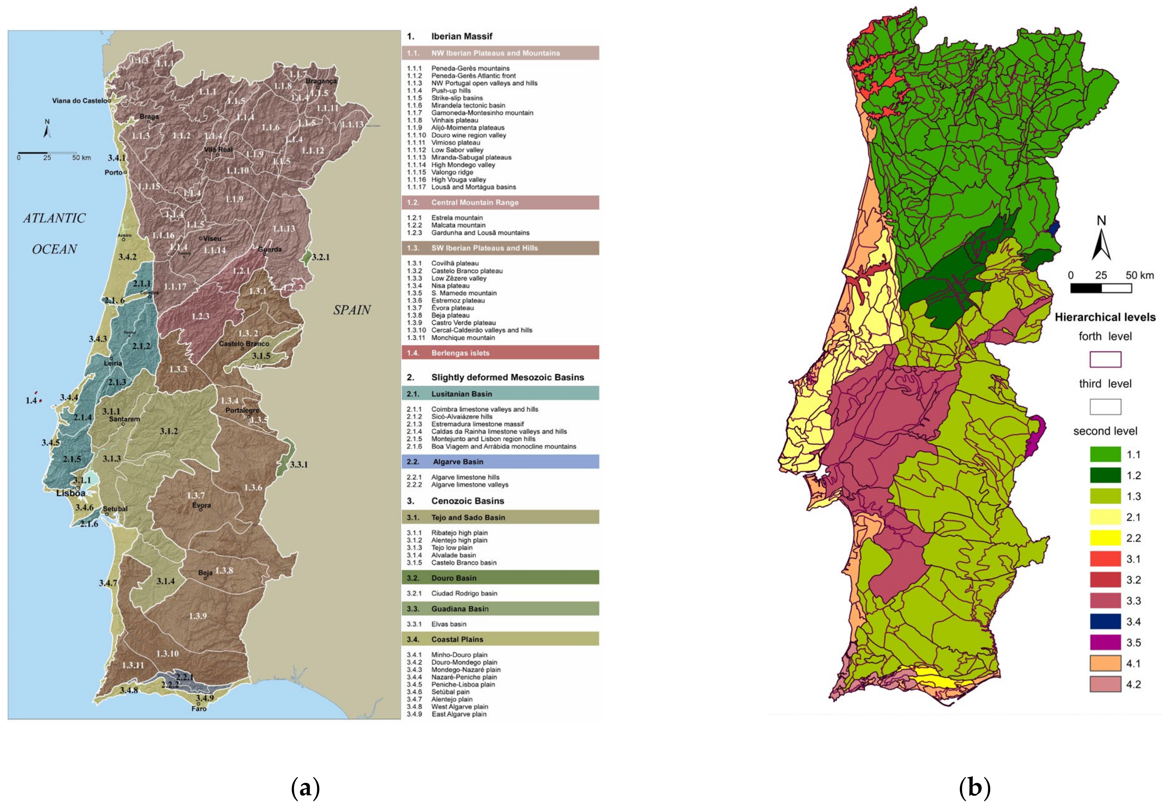
2.1.1. Geology

2.1.2. Geomorphology
2.2. Methodology
3. Results
3.1. Lithological Indices–Statistical Parameters
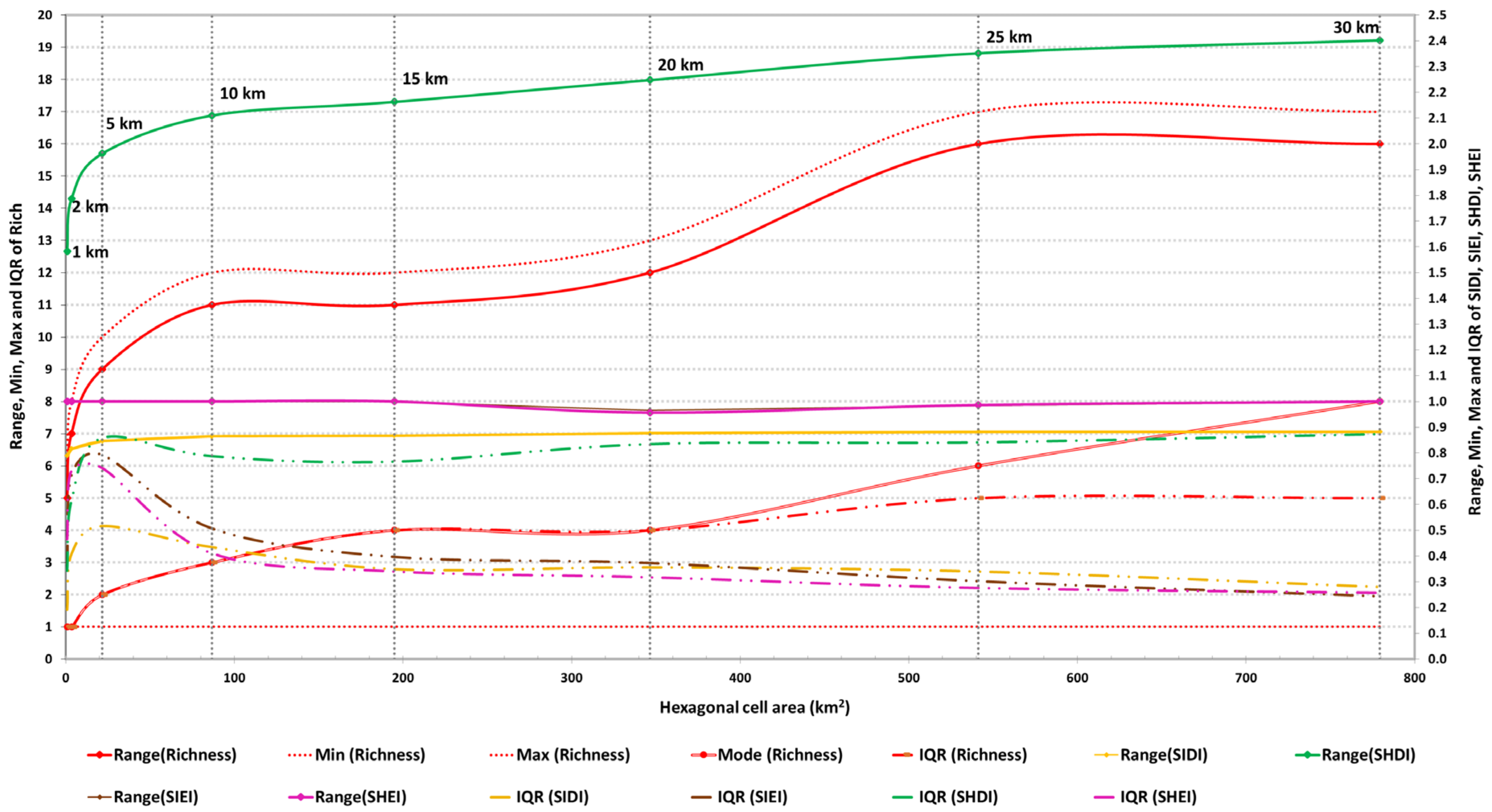
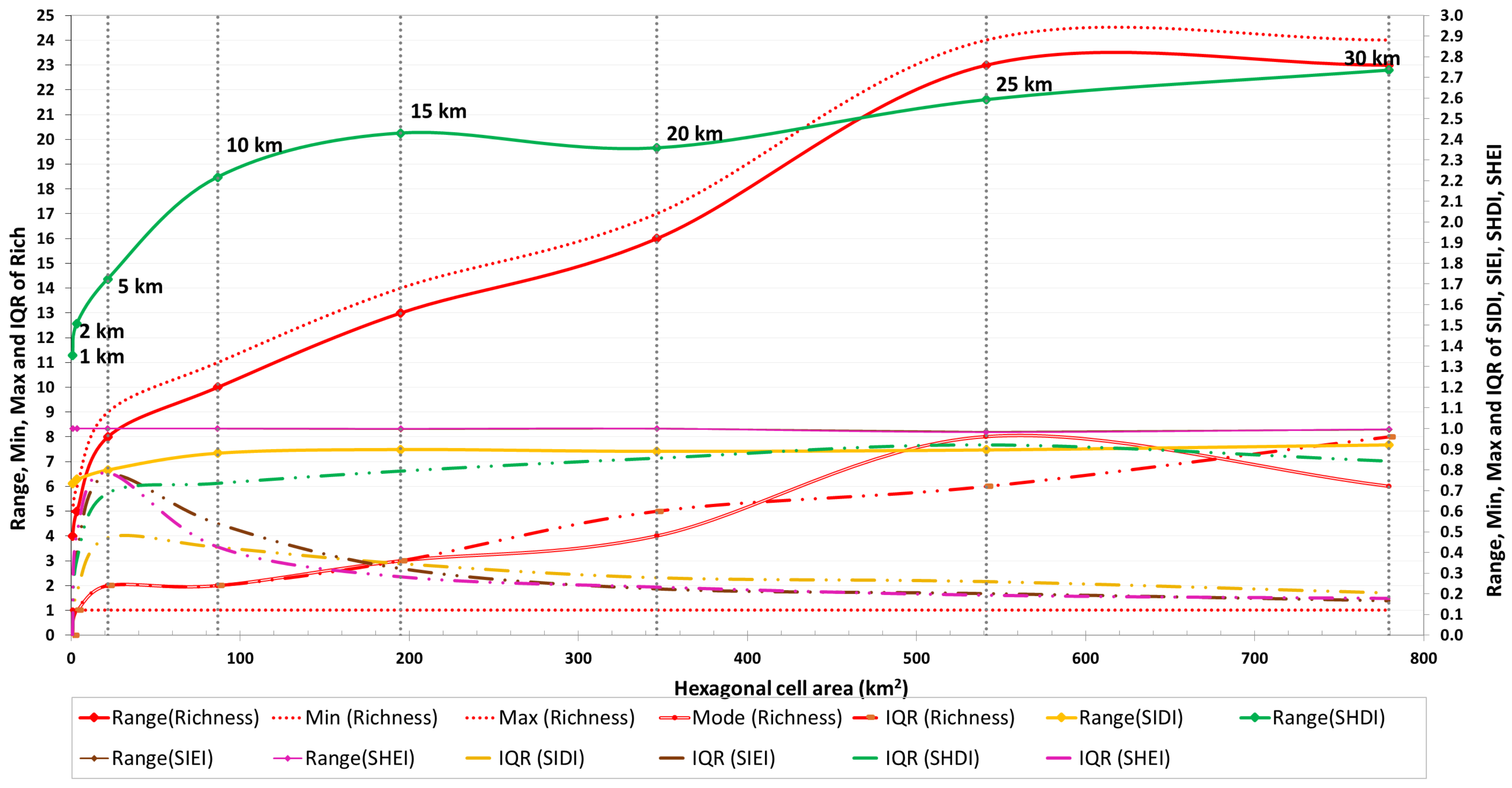
3.1.1. Mode, Range, Min, Max and IQR
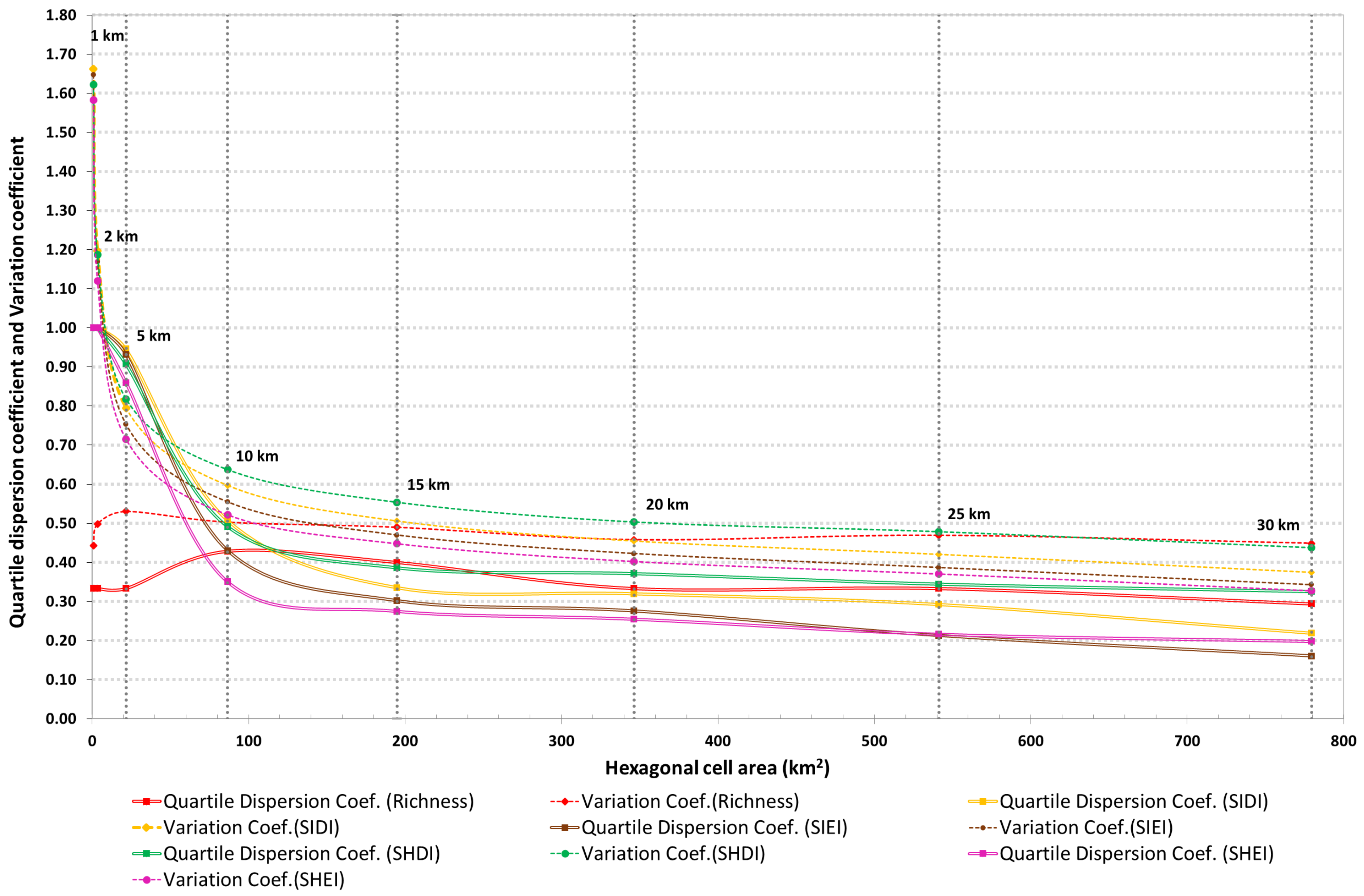
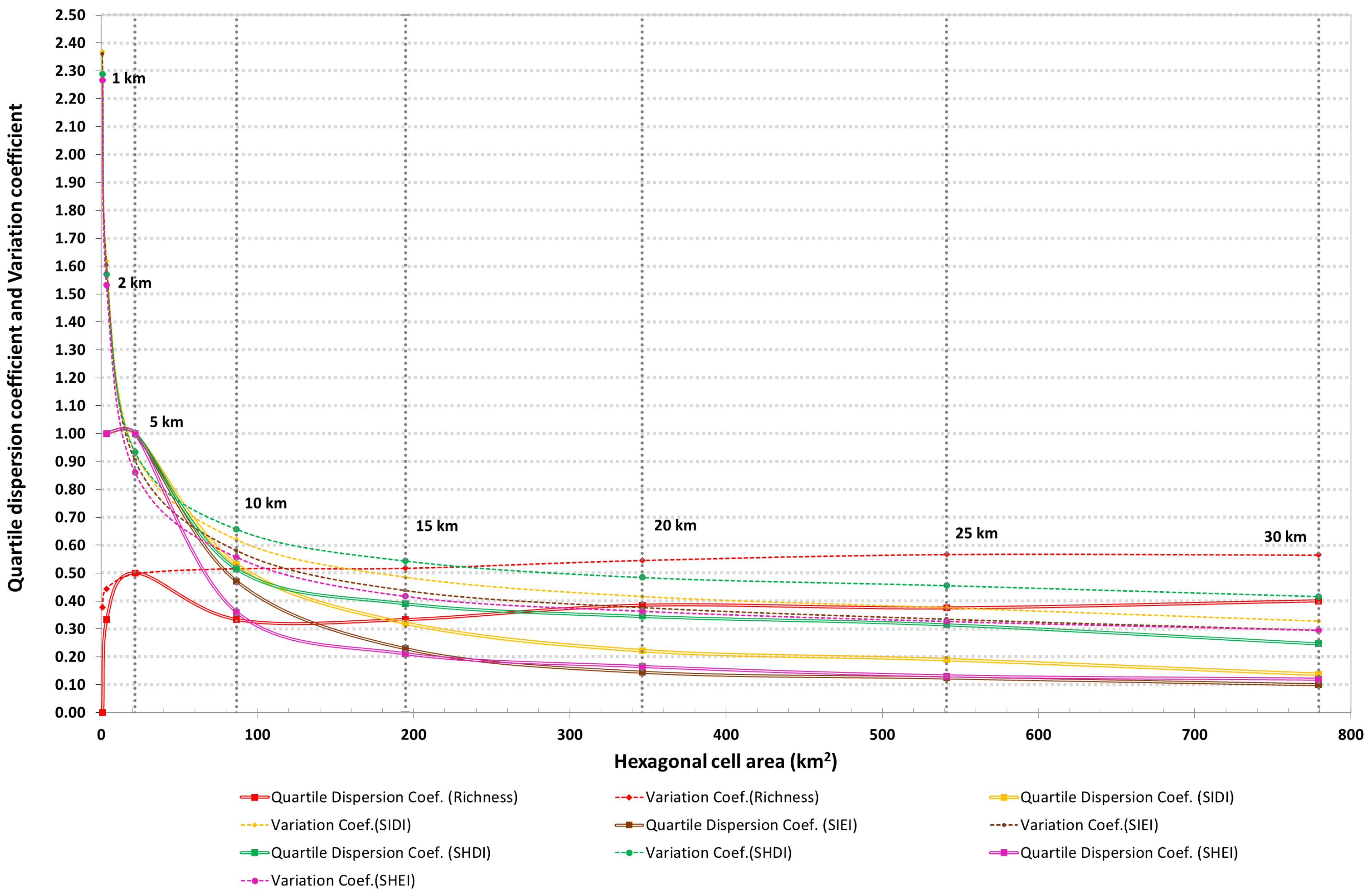
3.1.2. Quartile Coefficient of Dispersion and Coefficient of Variation
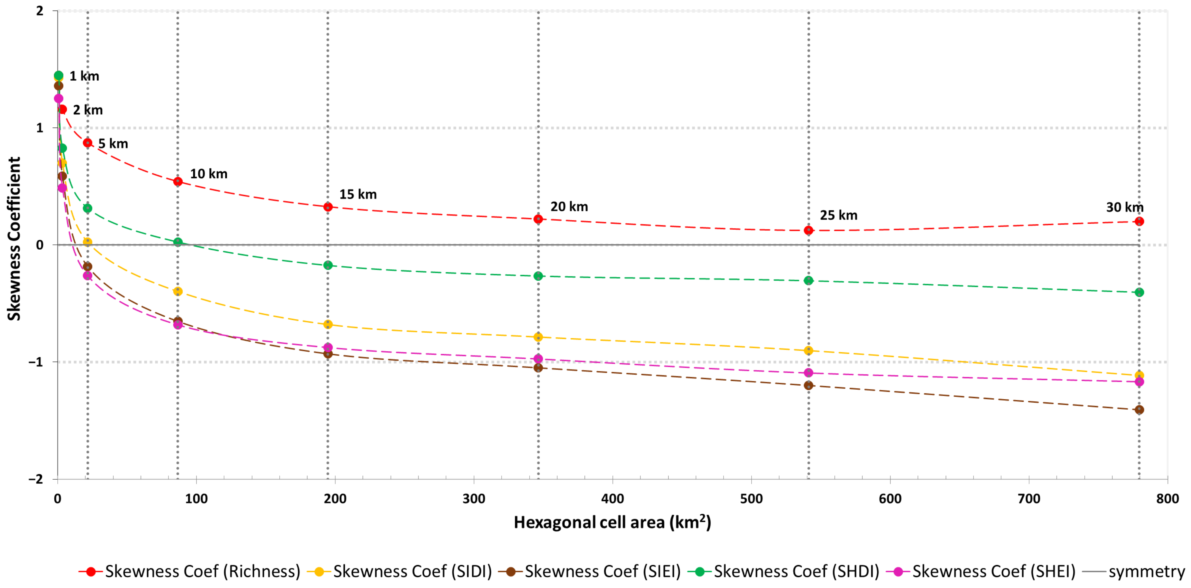
3.1.3. Skewness Coefficient
3.2. Geomorphological Indices–Statistical Parameters
3.2.1. Mode, Range, Min, Max and IQR
3.2.2. Quartile Coefficient of Dispersion and Coefficient of Variation
3.2.3. Skewness Coefficient
3.3. Correlation Factors (Lithological and Geomorphological Indices)
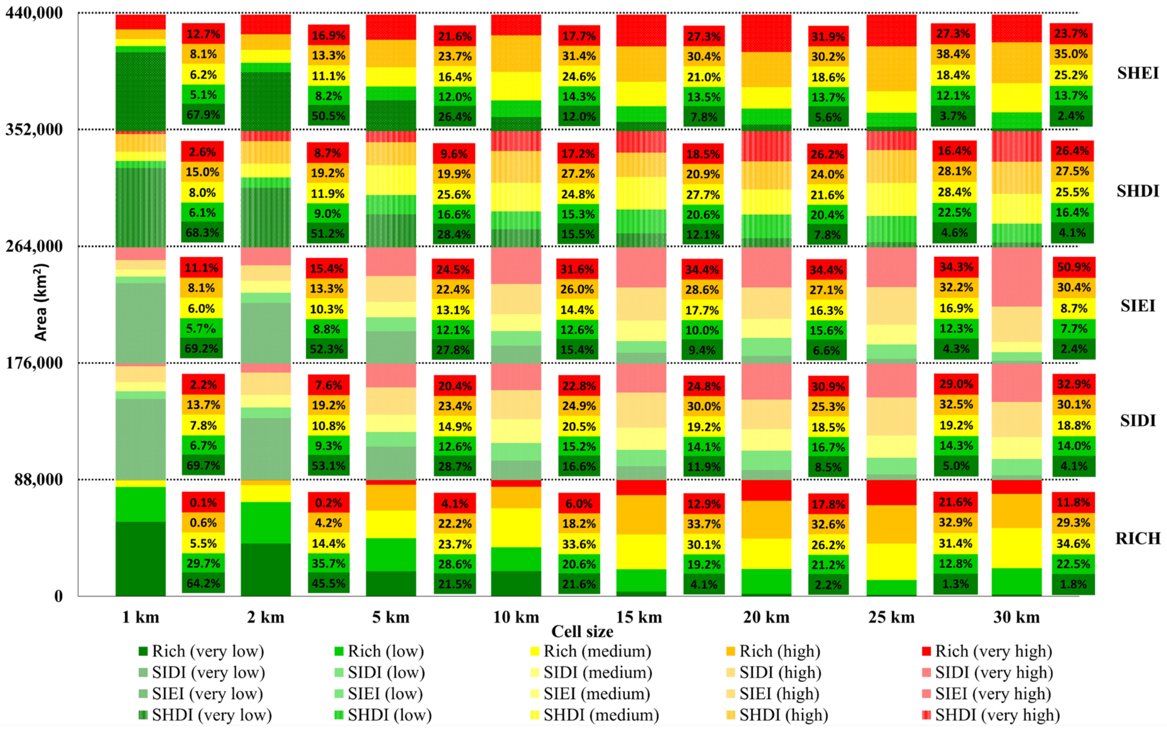
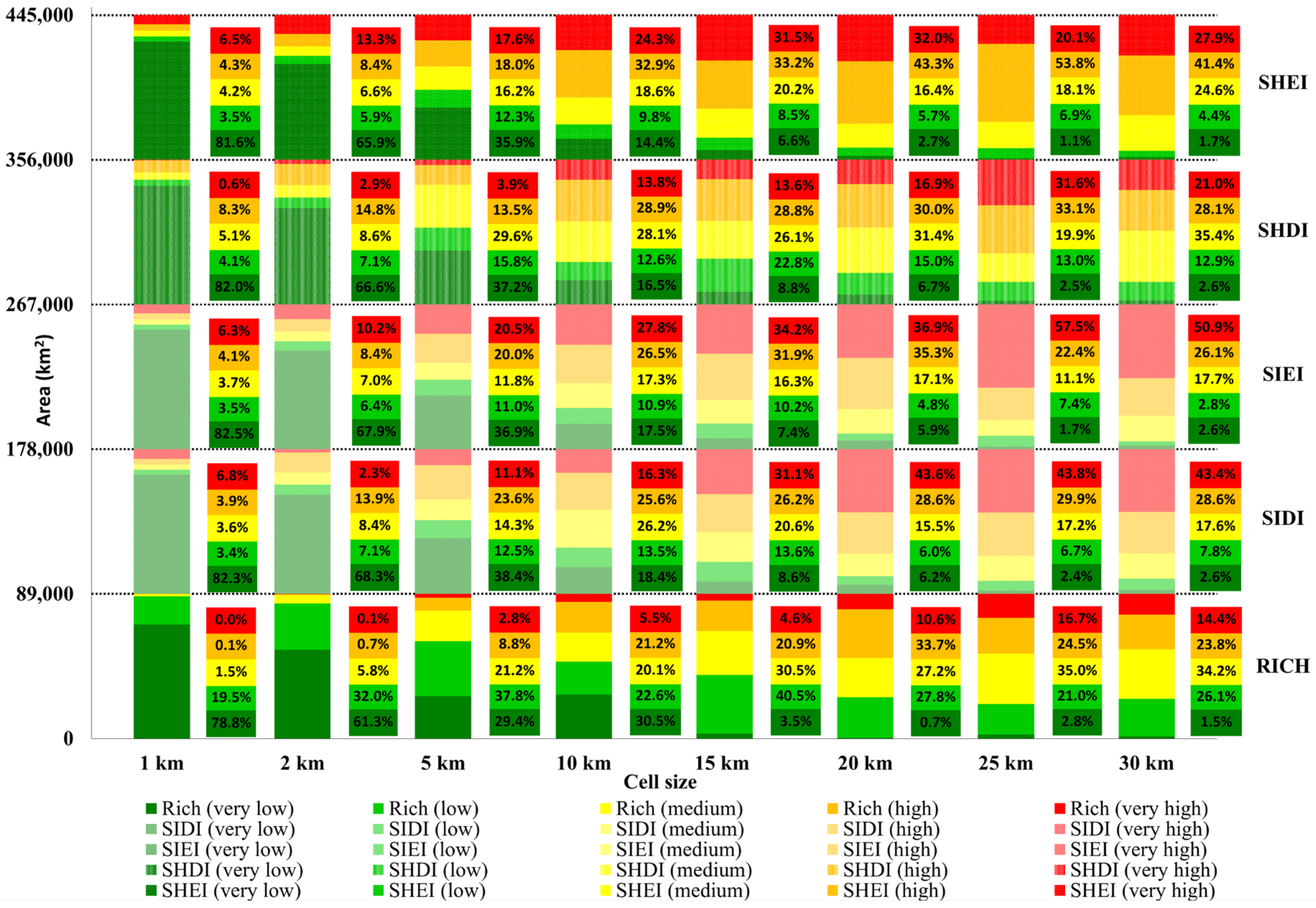
3.4. Lithological and Geomorphological Indices: Maps
3.4.1. Lithological Indices: Maps
3.4.2. Geomorphological Indices: Maps
4. Discussion
4.1. Cell Size
4.2. Statistic Parameters as Indicators
4.3. Indices as Cell Size Indicators and Geodiversity Assessors
4.4. Other Methods and Applicability
5. Conclusions
Supplementary Materials
Author Contributions
Funding
Acknowledgments
Conflicts of Interest
References
- Gray, M. Geodiversity: Valuing and Conserving Abiotic Nature, 2nd ed.; Wiley Blackwell: Chichester, UK, 2013; p. 512. ISBN 978-0-470-74215-0. [Google Scholar]
- Sharples, C. Concepts and Principles of Geoconservation, 3rd ed.; Tasmanian Parks & Wildlife: Hobart, Australia, 2002; p. 81. [Google Scholar]
- Nieto, L. Geodiversidad: Propuesta de una definición integradora. Bol. Geol. Min. 2001, 112, 3–12. [Google Scholar]
- Serrano, E.; Ruiz-Flaño, P. Geodiversity: A theoretical and applied concept. Geogr. Helv. 2007, 62, 140–147. [Google Scholar] [CrossRef]
- Kozlowski, S. Geodiversity: The concept and scope of geodiversity. Prz. Geol. 2004, 52, 833–837. [Google Scholar]
- Zarnetske, P.L.; Read, Q.D.; Record, S.; Gaddis, K.D.; Pau, S.; Hobi, M.L.; Malone, S.L.; Costanza, J.; Dahlin, K.M.; Latimer, A.M.; et al. Towards connecting biodiversity and geodiversity across scales with satellite remote sensing. Glob. Ecol. Biogeogr. 2019, 28, 548–556. [Google Scholar] [CrossRef]
- Pellitero, R.; Manosso, F.C.; Serrano, E. Mid- and large-escale geodiversity calculation in Fuentes-Carrionas (NW Spain) and Serra do Cadeado (Paraná, Brazil): Methodology and application for land management. Geogr. Ann. Ser. A Phys. Geogr. 2014, 97, 19–235. [Google Scholar] [CrossRef]
- Zwoliñski, Z.; Najwer, A.; Giardino, M. Methods for assessing geodiversity. In Geoheritage: Assessment, Protection, and Management; Reynard, E., Brilha, J., Eds.; Elsevier: Amsterdam, The Netherlands, 2018; pp. 27–47. [Google Scholar]
- Brilha, J.; Gray, M.; Pereira, D.I.; Pereira, P. Geodiversity: An integrative review as a contribution to the sustainable management of the whole of nature. Environ. Sci. Policy 2018, 86, 19–28. [Google Scholar] [CrossRef]
- Zwolinski, Z. The routine of landform geodiversity map design for the Polish Carpathian Mts. Landf. Anal. 2009, 11, 79–87. [Google Scholar]
- Zwolinski, Z.; Stachowiak, J. Geodiversity map of the Tatra National Park for geotourism. Quaest. Geogr. 2012, 31, 99–107. [Google Scholar] [CrossRef]
- Jankowski, P.; Najwer, A.; Zwoliński, Z.; Niesterowicz, J. Geodiversity Assessment with Crowdsourced Data and Spatial Multicriteria Analysis. ISPRS Int. J. Geo-Inf. 2020, 9, 716. [Google Scholar] [CrossRef]
- Najwer, A.; Borysiak, J.; Gudowicz, J.; Mazurek, M.; Zwoliński, Z. Geodiversity and Biodiversity of the Postglacial Landscape (Dębnica River Catchment, Poland). Quaest. Geogr. 2016, 35, 5–28. [Google Scholar] [CrossRef]
- Najwer, A.; Jankowski, P.; Niesterowicz, J.; Zwoliński, Z. Geodiversity assessment with global and local spatial multicriteria analysis. Int. J. Appl. Earth Obs. Geoinf. 2022, 107, 102665. [Google Scholar] [CrossRef]
- Najwer, A.; Reynard, E.; Zwoliński, Z. Geodiversity assessment for geomorphosites management: Derborence and Illgraben, Swiss Alps. Geol. Soc. Lond. Spec. Publ. 2022, 530, 18. [Google Scholar] [CrossRef]
- Crisp, J.R.; Ellison, J.C.; Fischer, A. Current trends and future directions in quantitative geodiversity assessment. Prog. Phys. Geogr. Earth Environ. 2021, 45, 514–540. [Google Scholar] [CrossRef]
- Pereira, D.I.; Pereira, P.; Brilha, J.; Santos, L. Geodiversity assessment of Parana state (Brazil): An innovative approach. Environ. Manag. 2013, 52, 541–552. [Google Scholar] [CrossRef] [PubMed]
- Silva, J.; Rodrigues, C.; Pereira, D.I. Mapping and Analysis of Geodiversity Indices in the Xingu River Basin, Amazonia, Brazil. Geoheritage 2015, 7, 337–350. [Google Scholar] [CrossRef]
- Araújo, A.; Pereira, D.I. A New Methodological Contribution for the Geodiversity Assessment: Applicability to Ceará State (Brazil). Geoheritage 2018, 10, 591–605. [Google Scholar] [CrossRef]
- Gonçalves, J.; Mansur, K.; Santos, D.; Henriques, R.; Pereira, P. A discussion on the quantification and classification of geodiversity indices based on GIS methodological tests. Geoheritage 2020, 12, 1–20. [Google Scholar] [CrossRef]
- Gonçalves, J.; Mansur, K.; Santos, D.; Henriques, R.; Pereira, P. Is It Worth Assessing Geodiversity Numerically? A Comparative Analysis between Quantitative and Qualitative Approaches in Miguel Pereira Municipality, Rio de Janeiro, Brazil. Geosciences 2022, 12, 347. [Google Scholar] [CrossRef]
- Queiroz, D.S.; Garcia, M.G.M.; Pereira, P. Criteria for Selecting Areas to Identify Ecosystem Services Provided by Geodiversity: A Study on the Coast of São Paulo, Brazil. Resources 2022, 11, 92. [Google Scholar] [CrossRef]
- Forte, J.P.; Brilha, J.; Pereira, D.I.; Nolasco, M. Kernel Density Applied to the Quantitative Assessment of Geodiversity. Geoheritage 2018, 10, 205–2017. [Google Scholar] [CrossRef]
- Peixoto, R.M.F. Avaliação da Geodiversidade de Portugal Continental. Master’s Thesis, University of Minho, Braga, Portugal, 2021. [Google Scholar]
- Carcavilla, L.; López, J.; Durán, J. Patrimonio geológico y geodiversidad: Investigación, conservación, gestión y relación con los espacios naturales protegidos. In Cuadernos del MuseoGeominero; IGME: Madrid, Spain, 2007; p. 360. ISBN 978-84-7840-710-1. [Google Scholar]
- Gray, M. Geodiversity: Valuing and Conserving Abiotic Nature; Wiley: Chichester, UK, 2004. [Google Scholar]
- Ibánez, J.; Brevik, E. Geodiversity Research at the Crossroads: Two Sides of the Same Coin. Span. J. Soil Sci. 2022, 12, 10456. [Google Scholar] [CrossRef]
- Benito-Calvo, A.; Pérez-González, A.; Magri, O.; Meza, P. Assessing regional geodiversity: The Iberian Peninsula. Earth Surface Process. Landf. 2009, 34, 1433–1445. [Google Scholar] [CrossRef]
- Manosso, F.C.; Zwoliński, Z.; Najwer, A.; Basso, B.T.; Santos, D.S.; Pagliarini, M.V. Spatial pattern of geodiversity assessment in the Marrecas River drainage basin, Paraná, Brazil. Ecol. Indic. 2021, 126, 107703. [Google Scholar] [CrossRef]
- Bartuś, T. Basic unit size in the analysis of the distribution of spatial landscape elements on the basis of the lithostratigraphic geodiversity of the Ojców National Park (Poland). Geol. Geophys. Environ. 2018, 43, 95–108. [Google Scholar] [CrossRef]
- Kot, R. A comparison of results from geomorphological diversity evaluation methods in the Polish Lowland (Toruń Basin and Chełmno Lakeland). Geogr. Tidsskr.-Dan. J. Geogr. 2017, 118, 17–35. [Google Scholar] [CrossRef]
- Nasiri, A.; Shafiei, N.; Zandi, R. Evaluation of Geodiversity Across Noorabad Basin (Fars Province, Iran). Geoheritage 2022, 14, 119. [Google Scholar] [CrossRef]
- Burnett, M.R.; August, P.V.; Brown, J.H., Jr.; Killingbeck, K.T. The influence of geomorphological heterogeneity on biodiversity. A patch-scale perspective. Conserv. Biol. 1998, 12, 363–370. [Google Scholar] [CrossRef]
- Nichols, W.; Killingbeck, K.; August, P. The influence of geormorphological heterogeneity on biodiversity. A landscape perspective. Conserv. Biol. 1998, 12, 371–379. [Google Scholar] [CrossRef]
- McGarigal, K.; Marks, B.J. FRAGSTATS: Spatial Pattern Analysis Program for Quantifying Landscape Structure; USDA Forest Service General Technical Report PNW-351; USDA: Corvallis, OR, USA, 1995.
- Shannon, C.; Weaver, W. The Mathematical Theory of Communication; University of Illinois Press: Urbana, IL, USA, 1949; p. 117. [Google Scholar]
- Simpson, E.H. Measurement of Diversity. Nature 1949, 163, 688. [Google Scholar] [CrossRef]
- Hengl, T. Finding the right pixel size. Comput. Geosci. 2006, 32, 1283–1298. [Google Scholar] [CrossRef]
- Marceau, D. The scale issue in social and natural sciences. Can. J. Remote Sens. 1999, 25, 347–356. [Google Scholar] [CrossRef]
- Florinsky, I.; Kuryakova, G. Determination of grid size for digital terrain modelling in landscape investigations—Exemplified by soil moisture distribution at a micro-scale. Int. J. Geogr. Inf. Sci. 2000, 14, 815–832. [Google Scholar] [CrossRef]
- Eiden, G.; Kayadjanian, M.; Vidal, C. Quantifying Landscape Structures: Spatial and Temporal Dimensions, in From Land Cover to Landscape Diversity in the European Union. Report of the European Commission. 2000. Available online: https://publications.jrc.ec.europa.eu/repository/bitstream/JRC32227/lbna21669enc.pdf (accessed on 8 March 2023).
- Bishop, T.F.A.; McBratney, A.B.; Whelan, B.M. Measuring the quality of digital soil maps using information criteria. Geoderma 2001, 103, 95–111. [Google Scholar] [CrossRef]
- Wickham, J.D.; Rhtters, K.H. Sensitivity of landscape metrics to pixel size. Int. J. Remote Sens. 1995, 16, 3585–3594. [Google Scholar] [CrossRef]
- Wu, J. Effects of changing scale on landscape pattern analysis: Scaling relations. Landsc. Ecol. 2004, 19, 125–138. [Google Scholar] [CrossRef]
- Bollati, I.M.; Cavalli, M. Unraveling the relationship between geomorphodiversity and sediment connectivity in a small alpine catchment. Trans. GIS 2021, 25, 2481–2500. [Google Scholar] [CrossRef]
- Rong, T.; Xu, S.; Lu, Y.; Tong, Y.; Yang, Z. Quantitative Assessment of Spatial Pattern of Geodiversity in the Tibetan Plateau. Sustainability 2023, 15, 299. [Google Scholar] [CrossRef]
- Bailey, J.J.; Boyd, D.S.; Hjort, J.; Lavers, C.P.; Field, R. Modelling native and alien vascular plant species richness: At which scales is geodiversity most relevant? Glob. Ecol. Biogeogr. 2017, 26, 763–776. [Google Scholar] [CrossRef]
- Barthlott, W.; Hostert, A.; Kier, G.; Kueper, W.; Kreft, H.; Mutke, J.; Rafiqpoor, M.; Sommer, J.H. Geographic patterns of vascular plant diversity at global to continental scales. Erdkunde 2007, 61, 305–315. [Google Scholar] [CrossRef]
- Hjort, J.; Heikkinen, K.; Luoto, M. Inclusion of explicit measures of geodiversity improve biodiversity models in a boreal landscape. Biodiv. Conserv. 2012, 21, 3487–3506. [Google Scholar] [CrossRef]
- Ribeiro, A.; Antunes, M.T.; Ferreira, M.P.; Rocha, R.B.; Soares, A.F.; Zbyszewski, G.; Moitinho de Almeida, F.; Carvalho, D.; Monteiro, J.H. Introduction à la Géologie Générale du Portugal; Serviços Geológicos de Portugal: Lisboa, Portugal, 1979; p. 114. [Google Scholar]
- Quesada, C. Evolución Tectónica del Maciço Ibérico. In Paleozoico Inferior de Ibero-América; Gutierrez-Marco, J.G., Saavedra, J., Rábano, I., Eds.; Universidad de Extremadura: Badajoz, Spain, 1992; pp. 173–190. [Google Scholar]
- Ribeiro, A. Evolução da Geodinâmica de Portugal; uma introdução. In Geologia de Portugal. Volume I Geologia Pré-Mesozóica de Portugal; Dias, R., Araújo, A., Terrinha, P., Kullberg, J., Eds.; Escolar Editora: Lisboa, Portugal, 2013; pp. 7–10. [Google Scholar]
- Ribeiro, A.; Dias, R.; Mateus, A.; Relvas, J.; Pinto, Á.; Romão, J. Geodynamics of Iberia, supercontinent cycles and metallogenic implications. Comun. Geológicas 2014, 101, 293–296. [Google Scholar]
- Dias, R. Portugal de Antes da História. Volume 1: Da Dinâmica Global aos Processos Geológicos, 1st ed.; Centro Ciência Viva de Estremoz: Estremoz, Portugal, 2019; p. 439. ISBN 978-989-95398-6-0. [Google Scholar]
- Kullberg, J.C.; da Rocha, R.B.; Soares, A.F.; Duarte, L.V.; Marques, J.F. Palaeogeographical Evolution of the Lusitanian Basin (Portugal) During the Jurassic. Part I: The Tectonic Constraints and Sedimentary Response. In Proceedings of the 1st International Congress on Stratigraphy (STRATI 2013), Lisbon, Portugal, 1–7 July 2013; pp. 665–672. [Google Scholar] [CrossRef]
- Dias, R.; Araújo, A.; Terrinha, P.; Kullberg, J.C. (Eds.) Geologia de Portugal. Volume I Geologia Pré-Mesozóica de Portugal; Escolar Editora: Lisboa, Portugal, 2013; p. 807. [Google Scholar]
- Dias, R.; Araújo, A.; Terrinha, P.; Kullberg, J.C. (Eds.) Geologia de Portugal. Volume II Geologia Meso-Cenozóica de Portugal; Escolar Editora: Lisboa, Portugal, 2013; p. 798. [Google Scholar]
- Ribeiro, M.L.; Bento dos Santos, T. A nova Carta Geológica de Portugal à Escala 1:1.000.000 e a Importância da Cartografia Geológica de Base. In: Portugal Tecnológico 2010, Lisboa, 24 de Setembro de 2010. Available online: http://hdl.handle.net/10400.9/1034 (accessed on 8 March 2023).
- National Laboratory of Energy and Geology. Carta Geológica de Portugal à Escala 1:1000000, Edição 2010; LNEG-LGM: Lisboa, Portugal, 2010; ISBN 978-989-675-005-3. [Google Scholar]
- Ferreira, A.M.P.J. Dados Geoquímicos de Base de Sedimentos Fluviais de Amostragem de Baixa Densidade de Portugal Continental: Estudo de Factores de Variação Regional. Ph.D. Thesis, University of Aveiro, Aveiro, Portugal, 2000. Available online: http://hdl.handle.net/10400.9/542 (accessed on 8 March 2023).
- Martins, L.; Borralho, V. Mineral Potential of Portugal; Geological and Mining Institute: Lisbon, Portugal, 1998; p. 60. [Google Scholar]
- Romão, J.M.C.; Cunha, T.A. Cartografia geológica: Uma mais-valia para o desenvolvimento do território. Geonovas 2012, 25, 3–17. Available online: http://hdl.handle.net/10400.9/1770 (accessed on 8 March 2023).
- Ribeiro, O.; Lautensach, H.; Daveau, S. Geografia de Portugal. Volume 1: A Posição Geográfica e o Território; Edições João Sá da Costa: Lisboa, Portugal, 1987; p. 334. [Google Scholar]
- Ferreira, D.B. Carte Géomorphologique du Portugal; Memória Centro de Estudos Geográficos: Lisboa, Portugal, 1981; Volume 6, 53p. [Google Scholar]
- Feio, M.; Daveau, S. O Relevo de Portugal; Associação Portuguesa de Geomorfólogos: Coimbra, Portugal, 2004; 151p. [Google Scholar]
- Ferreira, A.B. Geografia de Portugal, Volume I. O Ambiente Físico; Círculo de Leitores: Lisboa, Portugal, 2005; 495p. [Google Scholar]
- Pereira, D.I.; Pereira, P.J.S.; Santos, L.J.C.; da Silva, J.M.F. Unidades Geomorfológicas de Portugal Continental. Rev. Bras. Geomorfol. 2014, 15, 567–584. [Google Scholar] [CrossRef]
- Ramos, C.; Ramos-Pereira, A. Landscapes of Portugal: Paleogeographic Evolution, Tectonics and Geomorphology. In Landscapes and Landforms of Portugal; Vieira, G., Zêzere, J., Mora, C., Eds.; World Geomorphological Landscapes; Springer: Cham, Switzerland, 2020; pp. 3–31. [Google Scholar] [CrossRef]
- Datta, K. Does geodiversity correlate with land use/land cover diversity? A case study of Birbhum district, West Bengal, India. Proc. Geol. Assoc. 2022, 133, 589–602. [Google Scholar] [CrossRef]
- Ilić, M.; Stojković, S.; Rundić, L.; Ćalić, J.; Sandić, D. Application of the geodiversity index for the assessment of geodiversity in urban areas: An example of the Belgrade city area, Serbia. Geol. Croat. 2016, 69, 325–336. [Google Scholar] [CrossRef]
- Seijmonsbergen, A.C.; Guldenaar, J.; Rijsdijk, K.F. Exploring Hawaiian long-term insular geodiversity dynamics. Landf. Anal. 2018, 35, 31–43. [Google Scholar] [CrossRef]
- Seijmonsbergen, A.C.; Valentijn, S.; Westerhof, L.; Rijsdijk, K.F. Exploring Ocean Floor Geodiversity in Relation to Mineral Resources in the Southwest Pacific Ocean. Resources 2022, 11, 60. [Google Scholar] [CrossRef]
- Hjort, J.; Luoto, M. Geodiversity of high-latitude landscapes in northern Finland. Geomorphology 2010, 115, 109–116. [Google Scholar] [CrossRef]
- Nieto, L. Geodiversity as a Tool for the Nature Conservation. In Current Perspectives on Applied Geomorphology; IntechOpen: London, UK, 2023. [Google Scholar] [CrossRef]


| Cell_km (L) | Area Cell km2 | n Total | Empty | Filled |
|---|---|---|---|---|
| 30 | 779.4 | 345 | 195 | 150 |
| 25 | 541.3 | 442 | 230 | 212 |
| 20 | 346.4 | 620 | 305 | 315 |
| 15 | 194.9 | 1066 | 530 | 536 |
| 10 | 86.6 | 2379 | 1223 | 1156 |
| 5 | 21.7 | 9516 | 5150 | 4366 |
| 2 | 3.5 | 59,170 | 32,780 | 26,390 |
| 1 | 0.9 | 236,070 | 131,848 | 104,222 |
| Index | Formula | Range |
|---|---|---|
| Richness (Rich) | ||
| Shannon’s Diversity Index (SHDI) | ||
| Shannon’s Evenness Index (SHEI) | ||
| Simpson’s Diversity Index (SIDI) | ||
| Simpson’s Evenness Index (SIEI) |
Disclaimer/Publisher’s Note: The statements, opinions and data contained in all publications are solely those of the individual author(s) and contributor(s) and not of MDPI and/or the editor(s). MDPI and/or the editor(s) disclaim responsibility for any injury to people or property resulting from any ideas, methods, instructions or products referred to in the content. |
© 2023 by the authors. Licensee MDPI, Basel, Switzerland. This article is an open access article distributed under the terms and conditions of the Creative Commons Attribution (CC BY) license (https://creativecommons.org/licenses/by/4.0/).
Share and Cite
Lopes, C.; Teixeira, Z.; Pereira, D.I.; Pereira, P. Identifying Optimal Cell Size for Geodiversity Quantitative Assessment with Richness, Diversity and Evenness Indices. Resources 2023, 12, 65. https://doi.org/10.3390/resources12060065
Lopes C, Teixeira Z, Pereira DI, Pereira P. Identifying Optimal Cell Size for Geodiversity Quantitative Assessment with Richness, Diversity and Evenness Indices. Resources. 2023; 12(6):65. https://doi.org/10.3390/resources12060065
Chicago/Turabian StyleLopes, Catarina, Zara Teixeira, Diamantino I. Pereira, and Paulo Pereira. 2023. "Identifying Optimal Cell Size for Geodiversity Quantitative Assessment with Richness, Diversity and Evenness Indices" Resources 12, no. 6: 65. https://doi.org/10.3390/resources12060065